CHAPTER 3

DIGITAL SIGNAL PROCESSING INSTRUMENTATION

3.1 Signals and Signal Processing:

Signals play an important role in our daily life. Examples of signals that we encounter

frequently are speech, music, picture, and video signals. A signal is a junction of independent

variables such as time, distance, position, temperature, pressure. For example, speech and music

signals represent air pressure as a function of time at a point in a space. A black and white picture is

a representation of light intensity as function two spatial coordinates. The video signal in television

consists of sequence of images, called frames, and is function of three variables; two spatial

coordinates and time.

Most signals we encounter are generated by natural means. However, a signal can also be

generated synthetically or by computer simulation. A signal carries; information, and the objective

of signal processing is to extract the information carried by the signal. The method of information

extraction depends on the type of signal and the nature of information being carried by the signal.

Thus, roughly speaking, signal processing is concerned with the mathematical representation of the

signal and the algorithmic operation carried out on it to extract the information present. The

representation of the signal can be in terms of basis functions in the domain of the original

independent variable(s) or it can be in terms of basis functions in a transformed domain. Likewise,

the information extraction process may be carried out in the original domain of the signal or in a

transformed domain.

Depending on the nature of the independent variables and the value of the function defining

the signal, various types of signals can be defined. For example, independent variable can be

continuous or discrete. Likewise, the signal can either continuous or discrete function of the

independent variables. Moreover, the signal can be either a real valued function or a complex­

valued function.

62

A signal can be generated by a single source or by a multiple sources. In the former case, it

is a scalar signal and in the latter case it is a vector signal, often called multi channel signal.

A one-dimensional (1-D) signal is a function of a single independent variable. A two

dimensional (2-D) signal is a function of two independent variables. A multidimensional (M-D)

signal is a function of more than two variables.

The speech signal is an example of a 1-D signal where the independent variable is time An image

signal, such as a photograph, is an example of a 2-D signal where the two independent variables are

spatial variables. Each frame of black-and-white signal is a 2-D image signal that is a function of

two discrete spatial variables, with each frame occurring sequentially at discrete instants of time.

Hence, the black-and-white video signal must be considered as an example of three dimensional

(3-D) signal where the three independent variables are the two spatial variables and time. A colour

video signal is a three-channel signal composed of three 3-D signals representing the three primary

colours: red, green, and blue (RGB). For transmission purpose, the RGB television signal is

transformed into another type of three-channel signal composed of a luminance component and two

chrominance components.

The value of the signal at specific values of the independent variable(s) is called its

amplitude. The variation of the amplitude as a function of the independent variable(s) is called

waveform.

For a 1-D signal, the independent variable is usually labeled as time. If the independent

variable is continuous, the signal is called continuous-time signal. If the independent variable is

discrete, the signal is called discrete-time signal. A -time signal is defined at every instant of time.

On the other hand, a discrete-time signal is defined at the discrete instants of time, and hence, it is a

sequence numbers.

A continuous time signal with a continuous amplitude is usually called an analog signal. A

speech signal is an example of an analog signal. Analog signals are commonly encountered in our

daily life and are usually generated by natural means. A discrete-time signal with discrete-valued

63

amplitudes represented by a finite number of digits is referred to as a digital signal. An example of a

digital signal is the digitized music signal stored in a CD-ROM disk. A discrete-time signal with

continuous-valued amplitudes is called a sampled-data signal. This last type of signal occurs in

switched-capacitor (SC) circuits. A digital signal is thus a quantized sampled-data signal. Finally, a

continuous-time signal with discrete-valued amplitudes has been referred to as a quantized boxcar

signal. Figure(3.1) illustrates the four types of signals.

The functional dependence of a signal in its mathematical representation is often explicitly

shown. For a continuous-time 1 -D signal, the continuous independent variable is usually denoted by

t, whereas for a discrete-time 1 -D signal, the discrete independent variable is usually denoted by n.

For example, u(t) represents a continuous-time 1-D signal and (v[n]J represents a discrete-time 1-D

signal. Each member, v[n], of a discrete-time signal is called a sampling many applications, a

discrete-time signal is generated from a parent continuous-time signal by sampling the latter at

uniform intervals of time. If the discrete instants of time at which a discrete-time signal is defined

are uniformly spaced, the independent discrete variable n can be normalized to assume integer

values.

In the case of continuous-time 2-D signal, the two independent variables are the spatial

coordinates, which are usually denoted by x and y. For example, the intensity of a black-and-white

image can be expressed as u(x,y). On the other hand, a digitized image in 2-D discrete-time signal,

and its two independent variables are discretized spatial variables often denoted by m and n. Hence,

a digitized image can be represented as u(x,y,t) where x and y denote the two spatial variables and t

denotes the temporal variable time. A colour video signal is a vector signal composed of three

signals representing the three primary colours; red, green, and blue.

r(x,y,t)

u(x,y,t) = g(x,y,t) ..... (3.1)

b(x,y,t)

64

(O (d)

Fig 3-1 (a) A coniinuous-iime signal, (b) a digital signal, (c) a sampled-data signal, and (d) a quartfized boxcar signal.

65

There is another classification of signals that depends on certainty by which the signal can be

described. A signal that can be uniquely determined by a well-defined process such as a

mathematical expression or rule, or table look-up, is called a deterministic signal. A signal that is

generated in a random fashion cannot be predicted ahead of time is called random signal. However,

practical discrete-time systems employ finite word lengths for the storing of signals and the

implementation of signal processing algorithms, it is necessary to develop tools for the analysis of

finite length effects on the performance of discrete-time systems. To this end it has been found

convenient to represent certain pertinent signals as random signals and employ statistical techniques

for their analysis.

Some typical signal processing operations are reviewed in the following sections:

3.1.1 Typical Signal Processing Operations:

Various types of signal processing operations are employed in practice. In the case of analog

signals, most signal processing operations are usually carried out in the time-domain, whereas, in the

case of discrete-time signals, both time-domain and frequency domain operations are employed. In

either case, the desired operations are implemented by a combination of some elementary operations.

These operations are also usually implemented in real-time or near real-time, even though, in certain

applications, they may be implemented off-line.

The mathematical foundations on which the signal analysis is being performed is briefly

illustrated in the following sections - 3.2 Digital Signal Processing and 3.3 FFT Techniques.

3.2.1 INTRODUCTION TO DIGITAL SIGNAL PROCESSING [1 ]

Digital signal processing is an area of science and engineering that has developed rapidly

over the past four decades. The rapid development has been a result of the significant advances in

digital computer technology and integrated-circuit fabrication. The digital computers and associated

digital hardware has reached many users and is less expensive due to mass manufacturing of modem

computers and necessary hardware. From expensive and limited special usage of computers, a few

decades ago, the present personal computers are available at low affordable price (even to common

users in the form of Pcs). The rapid developments in the integrated -circuit technology, starting with

medium scale integration (MSI comprising of a few thousand transistor equivalents) to present day

66

Ultra Very Large Scale Integration (Ultra VLSI comprising a few billion thousand transistor

equivalents) that are produced in large quantities at very low cost are, smaller faster, and reliable.

The digital computers prepared using these devices are relatively fast digital circuits that highly

sophisticated digital systems capable of performing complex digital signal processing tasks. Using

equally reliable operating systems and software packages, the analog systems have been completely

replaced digital computer systems. The present work is perhaps a direct example of what is narrated

above. However some sections of scientific community are still not ready to adopt the new digital

systems. It is sufficient to state that many of the signal processing tasks that were conventionally

performed by analog means are realized today by less expensive and more reliable digital computer

firmware (the combination computer hardware and software).

However, signals with extremely wide bandwidths of real-time processing DSP is not a

replacement. For such applications analog or optical signal processing is the only possible solution.

Where necessary digital circuits of required speed are available, DSP are preferred. DSPs apart being

cheaper and more reliable, have other advantages of flexibility. The digital processing hardware are

usually programmable, and the programs can be easily altered as per to user requirements Through

software, one can more easily modify the signal processing functions to suit the performance of the

hardware. Higher precision is possible using the digital hardware (and the associated software)

compared to analog circuits and analog signal processing systems. Due to these advantages there

has been an explosive growth in the field of DSP and associated applications.

3.2.2. Frequency Analysis of Signals and DSPs:

The Fourier transform is one of the several mathematical tools that is useful in the analysis

and design of the so called LTI (Linear Time-Invariant) systems. These signal basically represent an

equivalent signal of known wave shape and distribution (sinusoidal or a complex exponent). With

such a decomposition, a signal is said to be represented in the frequency domain.

Most signals of practical interest [1] can be decomposed into a sum of sinusoidal signal

components. For the class of periodic signals, such a decomposition is often called as a Fourier

series. For the class of finite energy signals, the decomposition is called the Fourier transform.

These decompositions are of extreme importance. The LTI of sinusoidal signal input is a sinusoid of

the same frequency of different amplitude and phase. The linearity property of the LTI

67

systems implies that a linear sum of sinusoidal components, which produces a similar linear sum of

sinusoidal components at the output (which may differ in amplitudes and phases of the input

sinusoids). This characteristic behavior of LTI systems renders the sinusoidal decomposition. Many

other decompositions of signals are possible [2]. The class of sinusoidal (or complex exponential)

signals possess this desirable property in passing through an LTI system.

3.2.3 Tools Used in DSP Systems:

The tools required for frequency analysis of continuous periodic signals are briefly dealt

The best examples of periodic signals encountered in practice are: square waves, rectangular waves,

triangular waves, sinusoids and complex exponents. The basic mathematical representation of any

periodic signals is the well known Fourier series (a linear weighted sum harmonically related

sinusoids or complex exponents). Jean Baptise Joseph Fourier (1738-1830), a French mathematician

used trigonometric senes expansions in describing the phenomenon of heat conduction and

temperature distribution through bodies. The mathematical techniques so developed found

application in a variety of problems (encompassing the fields of optics, vibrations, mechanical

systems, system theory, and electromagnetics). This tool has been used for analysing functions

encountered in DSP. A linear combination of harmonically related complex exponents of the form

oox(t)= Z Cte^o' ... (3.2)

k = - oo

represents a periodic signal with fundamental period Tp=l/f). hence we can think of exponential signals { e ^2TTkf0l k = 0, ±1 ,±2,±3 ....} as the basic “building blocks” from which we can

construct periodic signals of various types by proper fundamental frequency and coefficients

(ck), f0 determines the fundamental period of x(t) and the coefficients {c*} specify the shape of

waveform. Suppose that we are given a periodic signal x(t) with period Tp we can represent the

periodic signal by the series, called a Fourier series, where the fundamental frequency fo is selected

to be the reciprocal of the given period Tp. To determine the expression for the coefficients (ct), we

first multiply both sides of (3.2) by the complex exponential

j2tTkf It W o

68

where 1 is an integer and then integrate both sides of resulting equation over a single period say

from 0 to Tp, are more generally, from to to to + Tp, where to is a arbitrary but mathematically

convenient value [3], Thus we obtain

10-Tp tO-Tp «

1 x(t) e j:n lfa dt = J x(t) e j:n,fc* (X ckej2nk f0< )dt ... (3.3)

|0 tO k

To evaluate the integral on the right-hand side of (3.3), we interchange the order of the summation

and integration and combine two exponentials. Hence

x to+Tp x to+TpX c„ Je)2n*** dt = £ c* / ****>] ... (3.4)

K = -x to k = -x to

for k ± 1, the right-hand side of (3.4) evaluated at the lower and upper limits , to and toDTp,

respectively, yields zero. On the other hand, if k = 1, we have

to+Tp to+Tp

J cat - [»]to to

consequently, (3.3) reduces to

to+Tpfx(t)e-j211 lfo,dt = c, Tp to

and therefore the expression for Fourier coefficients in terms of given periodic signal becomes

to+TpC-l/Tp f x(t)e'j2nifo,dt

to

since to is arbitrary, this integral can be evaluated over any interval of length Tp, i.e, over any

interval equal to the period of signal x(t). Consequently, the integral for Fourier series coefficients

will be written as

TPc, l/Tp|x(t)e-j2n,fo‘dt ... (3.5)

0

69

an important issue that arises in the representation of the period signal x(t) by the Fourier series is

whether or not the series converges to x(t) for every value of t i.e if the signal x(t) and its Fourier

senes representation

ocX cte j2rrkfo* ... (3.6)

k = - oc

are equal at every value at t. The so called Dirichlet conditions guarantee that the eqn (3 . / will b e

equal to x(t), except the values of t for which x(t) is discontinuous. At these values of‘t ‘ converges

to the mid point of a the discontinuity.

J|x(t)ldt<* ... (3.7)

T1 p

all periodic signals of practical interest satisfies this conditions.The weaker condition that signal has finite energy in one period,

{I x(t) 12dt < x ... (3.8)

T1 p

guarantees that the energy in the difference signal attains a value equal to zero through

CO

e(t) = x(t) - Ickej2TTkVk = - oc

Although x(t) and its Fourier series may not be equal for all values of t, eqn (3.7) implies eqn (3.8)

but not vice versa, eqns (3.7), (3.8) and Dirichlet conditions are sufficient but not necessary

conditions. This implies that the signals have Fourier series representation but do not fully satisfy

these conditions.

3.2.4 POWER DENSITY SPECTRUM OF PERIODIC SIGNALS

A periodic signal has infinite energy and a finite average power, which is given aspx = 1/Tp JI x(t) 12 dt <00

T1 p

(3-9)

70

if we take the complex conjugate of (3,2) and substitute for x(t) in (3.9) we obtain

px = 1/Tp J x(t) E cke * j2Trkfo'dt = Ic#k[l/TpJ x(t) e'j2TTkfo*dt ] ... (3.10)

Tp k = - « k = -oo Tp

^ I Ck I2

k = - x

therefore, we have established the relation

00

Px =inrp J Ix(t)|2dt<x = I,*,’ ... (3.11)Tp k = - x

which is called Parseval's relation for signal. To illustrate the physical meaning of eqn (3.11)

suppose that xk (t) consists of single complex exponential of the form

x(t) = ckej2TTkf0l

it can be shown that all Fourier series coefficients except ck are zero consequently, the average

power in the signal is

px I Ck |

It is obvious that | ck |2 represents the power in the k01 harmonic component [4] of the signal hence

the total average power in the periodic signal is simply the sum of the average power in all

harmonics.

If we plot the | Ck |2 as function of the frequencies kF0, k = 0, ±1 ,±2,±3 ....

the diagram that we obtain shows how the power periodic signal is distributed among the various

frequency components. Figure 3.2 illustrated below is known as “power density spectrum” of the

periodic signal x(t). Since the power in a periodic signal exits only at discrete values of frequencies

(i.e., F = 0, ± Fo, ± 2Fo, ± 3F0,...), the signal is said to have line spectrum. The spacing between

two consecutive spectral line is equal to the reciprocal of the fundamental period Tp, whereas the

shape of the spectrum (known as the power distribution of the signal), depends on the time-domain

characteristics of the signal. A typical power density spectrum is shown below:

71

-5F0 -4F0 -3F0 -2F0 -F0 0 F0 2 F0 3F0 4F0 5F0frf:quency

Fig 3.2 - Frequency versus jck]2, the modulus of the square Fourier coefficients (Power Spectral Density), a useful graph to identify the nature of the time distribution of signal

The Fourier series coefficients {ctj are complex valued , that is , they can be represented as Ck ~ 1 Ck I ej0k

where 0k = Z ck Instead of plotting the power density spectrum, we can plot the magnitude voltage

spectrum I Ck I and the phase spectrum 9k as functions of frequency. Clearly, the power spectral

density in the periodic signal is simply the square of the magnitude spectrum[5]. The phase

information is totally destroyed ( or does not appear ) in the power spectral density. If the periodic

signal is real valued, the Fourier series coefficients Ck satisfy the condition [6]C.k -C*k

Consequently, I CK 12 = I C \ 12. Hence the power spectrum is a symmetric function of frequency.

This condition also means that the magnitude spectrum is symmetric (even function )about the

origin and the phase spectrum is an odd function. As a consequence of the symmetry, it is sufficient

to specify that the spectrum of a real [7] periodic signal for positive frequencies only. The total

average power can be expressed as

oo

px = c20 +2 I I Ck |2 ...(3.12)k - *=c

72

= a2„ +l/2 I (a2k+b\) ... (3.13)

k - x

which follows directly from the relationships among {ak}, {bk} and fck) coefficients in the Fourier

senes expressions.

3.2.5 ENERGY DENSITY SPECTRUM OF APERIODIC SIGNAL

The energy density spectrum of a aperiodic signal can also be evaluated. Let x(t) be any finite signal

with Fourier transform X(F). Its energy is

X

Ex = J |x(t)|2dt-cc

which in turn be expressed in terms X(f)as follows

x

Ex — J x(t)x'(t) dt-X

cc

Ex = J |x(t)|2dt

-CC

which is known as parsevals relation for aperiodic, finite energy signals and expresses the principle

of conservation of energy in the time and frequency domains. The spectrum X(F) of signal is in

general, complex valued [8] consequently, it is usually expressed in the polar form:

X(F)= |x(F)| e,e<F)

where X(F) is the magnitude spectrum and © (F)= <X(F)

on the other hand, the quantity Sxx(F) = |x(F)| 2

which is in the integrand, represent the distribution of energy in the signal as a function of frequency

hence Sxx(F) is called energy density spectrum of X(t). The integral of S*x(F) over all frequencies

gives the total energy in the signal.

It can be easily shown that if the signal x(t) is real, then |x(-F)| =|x(F)|

< x(-F) = - < x(F)By combining eqn (3.14) & (3.15) we obtain

(3.14)(3.15)

73

Sxx(-F) = Sxx(F)(3.16)

in other words, the energy density spectrum of a real signal has even symmetry.

3.2.6 SAMPLING THEOREM REVISTED

To process a continuous time signal using signal processing technique, it is necessary to

convert the signal in to a sequence of numbers. This is usually done by sampling the analog signal,

say Xa(t), periodically every T seconds to produce [9] a discrete time signal x(n) given by

X(n)=Xa(nT) -oo <n < oo ... (3.17)

The relationship equ.(3.17) describes the sampling process in the time domain the sampling

frequency F, = 1/T must be selected large enough such that the sampling does not cause any loss of

information We investigate the sampling process by finding the relationship between the spectra of

signals Xa(t) and X(n). If X„(t) in an aperiodic signal with finite energy, its spectrum is given by the

Fourier transform relation

Xa(F) =f- X„(t) e'j2ilRdt ... (3.18)

where as the signal X,(t) can be recovered from its spectrum by the inverse Fourier transform

. X.(t)==J- Xa(F)e-j2nFtdF ... (3.19)

Note that utilization of all frequency components in the infinite range - oo < F < oo is necessary

to recover the signal Xa(t) if the signal Xa(t) is not band limited.

The spectrum of discrete-time signal x(n) is obtained by sampling X,(a) and its Fourier

transform is equal to:.

xX(<o)= Ix(n)e1“’ ... (3.20)

n = - xor, equivalently,

xX(f)= Zx(n)e'j2nfn ... (3.21)

n = - x

The sequence x(n) can be recovered [10] from its spectrum X(<d) or X(f) by the inverse transform

nx(n) = 1/2TI Jx(<B)e_J""do)

-n(3.22)

74

1/2

= J X(f>j2nfi,df ... (3,23)-1/2

In order to determine the relationship between the spectra discrete time signal and the analog

signal, we note that periodic sampling imposes a relationship between the independent variable t

and n in the signals xa(t) and x(n) respectively , that is

t = nT = n/F, ... (3.24)

This relationship in the domain implies a corresponding relationship between frequency

variables F and f in Xa(F) and X(f) respectively. Substitution of eqn (3.24) into eqn (3.19) yields

x(n) s xa(n T) = J Xa(F) ej2II,,F/Ts dF ... (3.25)•«

On comparing eqn (3.23) with eqn (3.25) we obtain

1 '2 OC

j X(f)ej21Ifndf = J Xa(F)eJ2"n,'T', dF ... (3.26)

-l a -oo

The periodic signal sampling imposes a relationship between frequency variables F and f of the

corresponding analog and discrete-time signals respectively. That is

f = F / F, (3.27)with the aid of (3.27), we can make simple change variable in eqn (3.26) and obtain the result

¥J2 oo

1/F, J x(F/F,) ej2ntfT5dF = J X8(F) ej2nnF/Fs dF ... (3.28)VJ2 -oo

we now turn our attention to the integral on the right-hand side of eqn (3.28). The integration range

of this integral can be divided into an infinite number of intervals of width F,. Thus the integral

over the finite range can be expressed as sum of integrals,

cc «i (It + ‘/2> fs

1 Xa(F)ej21lnF/Fs dF =Z Jxa(F)ej2rWs dF ... (3.29)

k -O’- k ; -ec (k * 1 i) fs

75

we observe that Xa(F) is in the frequency interval (K—l/2)Fs to (K+l/2)Fs and is identical to Xa(F- kFs) In the interval -Fs/2 to Fs/2. consequently,

x (k ' 'z)f* Fv2 «

I Jxs(F)eJ™dF = J [ IXa (F -kFs)] ej2r,aCTi dF ... (3.30)k -x (k * N)fs -i-%'2 -«

where we had used the periodicity of the exponential, namely, e j2n"ff+uvyF» _ e j2rinF?F»

This is the desired relationship between the spectrum X(F/Fs)or X(f) of the discrete time

signal and the spectrum Xa(F) of the analog signal [ 11 ]. the right hand side of eqn (3.31) or

eqn(3.32) consists of a periodic repetition of the scaled spectrum FsXa(F) with period Fs. This

periodicity is necessary because of spectrum X(f) or X(F/Fs) of the discrete time signal is periodic

with period fp =1 or Fp=Fs.

For example, suppose that the spectrum of a band limited analog signal is as shown in

Fig 3.3a The spectrum is zero for |F| > B. Now, if the sampling frequency Fs is selected to be greeter

than 2B, the spectrum X(F/Fs)of the discrete time signal will appear as shown inFig 3.3b .thus if the

sampling frequency Fs is selected such that Fs>2B is the Nquist rate, then

X(F/Fs) = FsXa(F) |F| < Fs/2 ... (3.31)

in this case there is no aliasing and therefore, the spectrum of the discrete time signal is identical

(with in the scale factor Fs) to the spectrum of the analog signal, with in the fundamental frequency

range |F| < Fs/2 or|F|<Fs/2or |fj < 1/2.

On the other hand, if the sampling frequency Fs is selected such that Fs<2B, the periodic continuation of Xa(F) results in spectral overlap, as illustrated in the Fig 3.3c and 3.3d. Thus the

spectrum X(F/Fs) of the discrete time signal contains aliased frequency components of the analog

signal spectrum Xa(F) the end result is that the aliasing which occurs prevents us from recovering

the original signal Xa(t) from the samples.

It is now possible to reconstruct the original analog signal from the samples X(n) by

considering

Xa(F) = {1 /Fs X(F/Fs), |F| < Fs/2 = 0 |F| > Fs/2

and the Fourier transform relationship equ(3.21) yields

(3.32)

76

(a)

(e)Fig 3.3 Sampling of an analog bandlimited signal and aliasing of spectral

components.

77

X(F/Fs) = SX(n) e'j2,IF“1'‘

The reconstruction of the original signal is hence possible and useful.

(3.33)

3.3 FUNDAMENTAL OF FAST FOURIER TRANSFOR (FFT) 1 \

The frequency analysis on a time domain signal function is performed using the well known

methods of Discrete Fourier Transform (DFT). DFT is a powerful computational tool. It plays an

important role in many applications of digital signal processing including linear filtering, correlation

analysis, and spectrum analysis. A major reason for its importance is the existence of efficient

algonthms for computing the DFT.

A few details of the algorithms for evaluating the DFT are presented. Two different

approaches are described. One is divide and conquer approach in which a DFT of size N is

computed (when the size N is a power of 2 or 4. The second approach is based on the formulation

of the DFT as a linear filtering operation on the data. This second approach leads to two algorithms,

the Goertzel algorithm and the chirp-z transform algorithm for computing the DFT via linear I)'w'f’N.

filtering of the data sequence.

3.3.1 COMPUTATION METHODS OF THE DFT AND FFT ALGORITHMS

Efficient methods of computing DFT are presented here. In view of the importance of the

DFT in various digital signal processing applications (linear filtering, correlation analysis and

spectrum analysis) this topic has received considerable attention by many mathematicians, engineers

and applied scientists[5]. The computational problem for the DFT is to computec^the sequence

{X(k)} of N complex numbers using given sequence of data (x(n)} of length N, which on

mathematical formulation turns out as

N-l’ knX(k) = I x(n) W1 N

n - 00 < k < N-l ... (3.34)

n - u

Where WK =ej2s/,! ... (3.35)

in general, the data sequence x(n) is also assumed to be complex valued. Similarly, the IDFT becomes

X(n) = 1/NS x(k) W ‘"kN * 'n = 0

0< k <N-1 (3.36).

T8

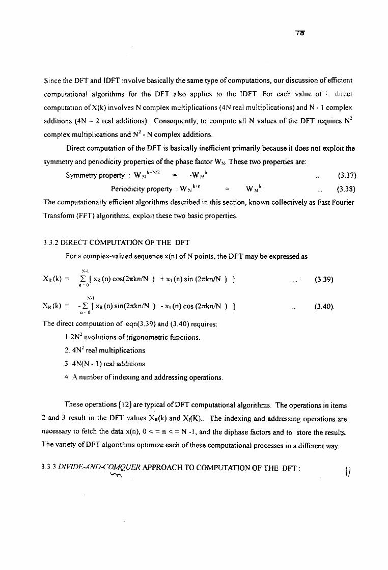
Since the DFT and IDFT involve basically the same type of computations, our discussion of efficient

computational algorithms for the DFT also applies to the IDFT. For each value of 1 direct

computation of X(k) involves N complex multiplications (4N real multiplications) and N -1 complex

additions (4N - 2 real additions). Consequently, to compute all N values of the DFT requires N2

complex multiplications and N2 - N complex additions.

Direct computation of the DFT is basically inefficient primarily because it does not exploit the

symmetry and periodicity properties of the phase factor WN. These two properties are:

Symmetry property : WNk+N?2 = -WNk ... (3.37)

Periodicity property : Wn*1’” = Wnk ... (3.38)

The computationally efficient algorithms described in this section, known collectively as Fast Fourier

Transform (FFT) algorithms, exploit these two basic properties.

3 3 2 DIRECT COMPUTATION OF THE DFT

For a complex-valued sequence x(n) of N points, the DFT

N-l

XR (k) = £ [ xr (n) cos(27ikn/N ) + x, (n) sin (27ckn/N ) ]n ' 0

N-l

Xr (k) = - Z { xr (n) sin(2rtkn/N ) - Xi (n) cos (27tkn/N ) ]n - ti

The direct computation of eqn(3.39) and (3.40) requires:

1 2N2 evolutions of trigonometric functions.

2. 4N2 real multiplications.

3. 4N(N - 1) real additions.

4. A number of indexing and addressing operations.

These operations [12] are typical of DFT computational algorithms. The operations in items

2 and 3 result in the DFT values XR(k) and Xi(K).. The indexing and addressing operations are

necessary to fetch the data x(n), 0< = n< = N- l, and the diphase factors and to store the results.

The variety of DFT algorithms optimize each of these computational processes in a different way.

3 3 3 DMDE-AND-COMQUER APPROACH TO COMPUTATION OF THE DFT : iWs )

may be expressed as

(3.39)

(3.40) .

79

The development of computationally efficient algorithms for the DFT is made possible if we

adopt a divided-and-conquer approach. This approach is based on the decomposition of an N-point

DFT into successively smaller DFTs. This basic approach leads to a family of computationally

efficient algorithms known collectively as FFT algorithms.

To illustrate the basic notions, let us consider the computation of an N-point DFT, where N

can be factored as a product of two integers, that is,

N = LM ...(3.40a)

The assumption that N is not a prime number is not restrictive, since we can pad any sequence with

zeros to ensure a factorization of the form (3.40a). Now the sequence x(n), 0 < n< N - 1, can be

stored in either a one-dimensional array indexed by n or as a two-dimensional array indexed by I and

m, where 0 < 1 < L-l and 0 < m < M-l as illustrated in Table 3.1.

Table 3 1 Two Dimensional Data Array For Storing the Sequence x(n), 0 < n < N-l

n 0 1 2 N-l

X(0) X(1) X(2) X(N-l)

\ m column index row \index / \ QJ_________ _________________________________________ M-l

1 x(0,0) x(0,1) x(0,2) x(0,M-l)

2 x(l,0) x(l,l) x(l,2) x(l,M-l)

3 x(2,0) x(2,l) x(2,2) x(2,M-l)

L-l x(L-l,0J x(L-l,l) x(L-l,2) (L-l,M-l)

80

Note that 1 is the row index and m is the column index. Thus the sequenced x(n) can be stored in a

rectangular array in a variety of ways, each of which depends on the mapping of index n to the

indexes (i,m).

For example, suppose that we select the mapping

n = M1 + m ... (3.41)

This leads to an arrangement in which the first row consists of the first M elements of x(n),

the second row consists of the next M elements of x(n), and so on, as illustrated in Table 3.1. On the

other hand, the mapping

n = 1 + mL ... (3.42)

stores the first L elements of x(n) in the first column, the next L elements in the second column, and

so on, as illustrated in Table 3.1 as a two dimensional array.

A similar arrangement can be used to store the computed DFT values. In particular, the

mapping is from the index k to a pair of indices (p,q), where 0 < p < L - 1 and 0 < q < M - 1. If we

select the mapping

k = Mp + q ... (3.43)

the DFT is stored on a row-wise basis, where the first row contains the first M elements of the DFT

X(k), the second row contains the next set of Md elements, and so on . On the other hand, the

mapping

k = qL + p ... (3.44)

results in a column-wise storage of X(k), where the first L elements are stored in the first column,

the second set of L elements are stored in the second column, and so on.

Now suppose that x(n) is mapped into the rectangular array x(l,m) and X(k) is mapped into a

corresponding rectangular array X(p,q). Then the DFT can be expressed as a double sum over the

elements of the rectangular array multiplied by the corresponding phase factors. To be specific let

us adopt a column-wise mapping for x(n) given by (3.42) and the row-wise mapping for the DFT

given by equ(3.44). Then

X(p,q) = I I xR(l,m) WN(Mp^)(raI- M) ... (3.45)m 0/0

But

81

WN(Mp*qx«L+t> = WnmL"pWn"MWn^ WnM (3.46)

However WNNn,p = I, WNmi q = WN/Lmq =

and ... (3.47)with these simplifications equ(3.45) can be expressed as

L 1 M-l

X(p,q) = I { [ L x(l,m) Wm”*] } ...(3.48)1-0 m- 0

The expression in eqn(3.48) involves computation of DFTs of length M and length L.To

elaborate, let us subdivide the computation in to three steps

1, First, we compute the M - DFTs

M-l

F(l,q) = X x(l,m) Wm"1, 0 < q < M-lm 0

for each other rows 1 = 0, 1,2 .. ..L-l.

2. Second we compute, a new rectangular array G(l„q) defined as

<3(1,q) = WNlqF(l,q) 0 < 1 < L-l 0 < q < M-l

3. Finally we compute the L - DFTs

L-l

X(p,q) = Z G(l,q) WLlp, ... (3.51)I “0

for each coloumn q = 0, 1,... M-1, of the array <3(1,q)

On the surface it may appear that the computational procedure outlined above is more

complex than the direct computation of the DFT. However, let us evaluate the computational

complexity of (3.48). The first step involves the computation of L DFTs, each of M points. Hence

(3.49)

(3.50)

82

this step requires LM2 complex multiplications and LM(M-1) complex additions. The second step

requires LM2 complex multiplications. Finally, the third step in the computation requires ML2

complex multiplications and ML(M-1) complex additions. Therefore, the computational complexity

is

Complex multiplications: N(M + L + 1)

Complex additions: N(M + L-2) ... (3.52)

where N = ML. Thus the number of multiplications has been reduced from N2 to N(M + L+l) and

the number of additions has been reduced from N(N-1) to N(M+L-2).

For example, suppose that N=1000 and we select L=2 and M=500. Then , instead of having to perform 106 complex multiplications via direct computation of the DFT, this approach leads to

503,000 complex multiplications. This represents a reduction by approximately a factor of 2. The

number of additions is also reduced by about a factor of 2.

When N is a highly composite number, that is, N can be factored into a product of prime

numbers of the form

N=rlr2...rv ... (3.53)

then the decomposition above can be repeated (v-1) more times. This procedure results in smaller

DFTs, which in turn, leads to a more efficient computational algorithm.

In effect, the first segmentation of the sequence x(n) into a rectangular array of Md columns

with L elements in each column resulted in DFTs of sizes L and M. Further decomposition of the

data in effect involves the segmentation of each row (or column) into smaller rectangular array

which result in smaller DFTs. This procedure terminates when N is factored into its prime factors.

To summarize, the algorithm that we have introduced involves following computations:

Algorithm 1

1 Store the signal column -wise.

2. Compute the M-point DFT of each row.3. Multiply the resulting array by the face factors Wlq„.

4 Compute the L-point DFT of each column.

5 Read the resulting array row-wise.

An additional algorithm with a similar computational structure can be obtained if the input

signal is stored row-wise and the resulting transformation is column-wise. In this case we select as

83

n = M I+m

k = q L+p ... (3.54)

This choice of indices leads to the formula for the DFT in the form

N-l /-IX (p,q) = II x(l,m) WNpm W,.1- W.T* ... (3 <5)

ID 0 / 0

N-l l-\X (p,q) = IWM““ [ I x(l,m) W,pl] WNpro ... (3.56)

m 0 (0

Thus we obtain a second algorithm.

Algorithm 2

1. Store the signal row-wise.

2. Compute the L-point DFT at each column.

3. Multiply the resulting array by the factors W >/“ .

4. Compute the M-point DFT of each row.

5. Read the resulting array column-wise.

The two algorithms given above have the same complexity. However, they differ in

the arrangement of the computations. In the following sections we exploit the divide-and-conquer

approach to derive fast algorithms when the size of the DFT is restricted to be a power of 2 or a

power of 4.

3 3 4 APPLICATIONS OF FFT ALGORITHMS

The FFT algorithms described in the preceding section [12] find application in a variety of

areas, including linear filtering, correlation, and spectrum analysis. Basically, the FFT algorithm is

used as an efficient means to compute the DFT and the IDFT.

In this section we consider the use of the FFT algorithm in linear filtering and in the

computation of the cross correlation of two sequences, we illustrate how to enhance the efficiency of

the FFT algorithm by forming complex-valued sequences from real-valued sequences prior to the

computation of the DFT,

Efficient Computation of the DFT of two Real Sequences

84

The FFT algorithm is designed to perform complex multiplications and additions, even

though the input data may be real valued. The basic reason for this situation is that the phase factors

are complex and hence, after the first stage of the algorithm, all variables are basically complex­

valued.

in view of the feet that the algorithm can handle complex-valued input sequences, we can

exploit this capability in the computation of the DFT of two real-valued sequences.

Suppose that xl (n) and x2(n) are two real-valued sequences of length N, and let x(n) be a

complex-valued sequence defined as

x(n) = xl(n)+jx2(n) 0<=n<=N-l ... (3.57)

The DFT operation is linear and hence the DFT of x(n) can be expressed as

X(k) = X,(k)+jX2(k) ... (3.58)

The sequences xl(n) and x2(n) can be expressed in terms of x(n) as follows: xt(n ) =( x(n)+ x(n)*)/2

x2(n) ={ x(n)- x(n)*)/2 ... (3.59)

hence the DFTs of xi(n) and x2(n) are

Xi(k) = l/2{DFT[x(n))+DFT[x*(n)]}

X2(k)= l/2|DFT[x(n)]-DFT[x*(n)]} ... (3.60)

OR X,(k)= l/2{x(k)]+[x*(N-k)]

X2(k)= l/2{x(k)]-[x*(N-k)] ... (3.61)

Thus, by performing a single DFT on the complex-valued sequence x(n), we have obtained

the DFT of the two real sequences with only a small amount of additional computation that is

involved in computing X1 (k) and X2(k) from X(k) by use of eqn (3.50) and (3.51).

3.3 5 EFFICIENT COMPUTATION OF THE DFT OF A 2N- POINT REAL SEQUENCE

Suppose that g(n) is a real-valued sequence of 2N points. We now demonstrate how to

obtain the 2N-point DFT of g(n) from computation of one N-point DFT involving complex, valued

data. First, we define

xi(n) = g(2n)

x2(n) = g(2n+l) ... (3.62)

Am

plitu

de

Am

plitu

de

85

20 40 60 80Time, msec

(b)

Bandpass filler output

100 20 40 60 SOTime, msec

(«)

Buds lop filler output

20 40 60 40 100Time, msec

(*)

Lowpsas filler output Hi(hpaas (iiter output

Input signal

A ..... i

20 40 60Tune, msec

SO 100 20 40 60Time, msec

80 100

. <d) (e)

Am

plitu

deo

*19

Am

plitu

de

o —

Fig 3.4 (a) Input signal, (b) ouipui of a lowpass filler with a cutoff al 80 Hr, (c) output of a high piss filter with t cutoff at 150 Hr, (d) output of a bandpass filter with cutoffs at 80 Hr and 150 Hr,' and (e) output of a bands lop filter with cutoffs at 80 Hr and 150 Hr.

86

Thus we have subdivided the 2N-point real sequence into two N-point real sequences, Now we can

apply the method described in the preceding section.

Let x(n) be the N-point complex-valued sequence

Thus we have computed the DFT of a 2N-point real sequence from one N-point DFT and

some additional computation as indicated above. The FFT method is hence useful to evaluate the

properties of variable signals even when signals are measured for a relatively short duration of time.

3.3.6 Filtering:

One of the most widely used complex signal processing operations is filtering. Filtering is

used to pass certain frequency components in a signal through the system without any distortion and

to block other frequency components. The system implementing this operation is called filter, range

of frequencies that is allowed to pass through the filter is called passband, the range of frequencies

that is blocked by the filter is called the stopband. Various types of filters can be defined, depending

on the nature of the filtering operation. In most cases, the filtering operation for analog signals is

linear and is described by the convolution integral

y(t)= y(t -1) x ( t ) dx ... (3.63)

where x(t) is the input signal and y(t) is the output of the filter characterized by an impulse response

h(t).

A lowpass filter passes all low-frequency components below a certain specification fa called

cutoff frequency, and blocks all high frequency components above fa A highpass filter passes all

high-frequency components above a certain cutoff frequency fc and blocks all low-frequency

components below fa A bandpass filter passes all frequency components between two cutoff

frequencies fa and fa, and blocks all frequency components below the frequency fa and above the

frequency fa. A bandstop filter blocks all frequency components between tow cutoff frequencies fa

and fa, and passes all frequency components below the frequency fa and above the frequence fa.

Figure 3.4(a) shows a signal composed of three sinusoidal components of frequencies 50Hz, 110Hz

87

and 210Hz, respectively Fig3.4(b) to (e) show the results of the above four types of filtering

operations with appropnately chosen cutoff frequencies.

A stopband filter designed to block a single frequency component is called notch filter. A

multiband filter has more than one passband and more than one stopband. A comb filter is designed

to block frequencies that are integral multiples of a low frequency.

A signal may get corrupted unintentionally by an interfering signal called interference or

noise. In many applications the desired signal occupies a low-frequency band from dc to some

frequency fL Hz, and it is corrupted by a high-frequency components above fH Hz with f» > fL. In

such cases, the desired signal can be recovered from the noise corrupted signal by passing the latter

through a low pass filter with a cutoff frequency fc where fi. < fc < fn„. A common source of noise ;s

power lines radiating electric fields. The noise generated by power lines radiating sinusoidal signal

corrupting the desired signal and can be removed by passing the corrupted signal through a notch

fiter with a notch frequency at 60 Hz.

3.3.7 Butterworth Approximation:

The magnitude-square response of an analog lowpass Butterworth filter H,(s) of Nth order is given

by

I Ha(jQ)l‘ =i/{i+(n/Qc)2Nj .... (3.64)

It can be easily shown that the first 2N-1 derivatives of |Ha( j f2)|2 at Q =0 are equal to zero, and as

a result, the Butterworth filter is said to have a maximally flat magnitude at Q =0. The gain of the

Butterworth filter in dB is given by

C(D) = 101ogl0|Ha(jQ)|2dB ... (3.65)

At dc, i.e., at Q =0, the gain in dB is equal to zero, and at Q = Q c, the gain is

88

C( Qe)= 10 log,o(l/2) =-3.0103 = -3 dB .... (3.66)

and therefore, Q c is often called the 3-dB cutoff frequency. Since the derivative of the companding

squared-magnitude response, or equivalently, of the magnitude response is always negative for

positive values of Q, the magnitude response, is monotonically decreasing with increasing Q. For

Q » Q c, the squared-magnitude function can be approximated by

where C, (Qi) is given by the gain in dB at Q,. As a result the gain roll-off per octave in the stopband

decreases by 6 dB, or equivalently, by 20 dB per decade of an increase of the filter order by one. In

other words, the passband and stopband behaviors of the magnitude response improve with a

corresponding decrease in the transition band as the filter order N increases. A plot of the magnitude

response of the normalized Butterworth lowpass filter with Q<.=1 for some typical values of N is

shown in fig 3.5

The tw<5 parameters completely characterizing a Butterworth filter are therefore the 3-dB

cutoff frequency Q c and the order N. These are determined form specified passband edge Qp, the

minimum passband magnitude 1/ V 1 + e2 the stopband edge Q,, and the maximum stopband ripple

1/A. Therefore can , we get

IH.0 qji2 * i/{( n/ a)2N} .... (3.67)

The gain Q Q2) in dB at Q 2 - 2Q t with fi, » Qc is given by

/;( Q2) = -20 logic ( Q2/ Qc)2N'= C( Q0-6N dB .... (3.68)

|H,(jQp)|2 = M{ 1 + ( Qp / a)2K} =l/( 1 +e2) .... (3.69)

ih8o a)i2 = i/{i + (a/ a)2N} = i/a: (3.70)

Solving the above we arrive at the expression for the order N as

89

N = log,o[(A2 - l)/e2] = logioCl/kj)2log10(£Vap) log,0(l/k)

Since the order N of the filter must be an integer, the value of N computed using the above

expression is rounded up to the next higher integer. This value of N can be used next in either

Eqn (3.63) or Eq.(3.64) to solve for the 3-dB cutoff frequency Qc If it is used in Eq.(3.63), the

passband specification is met exactly, whereas the stopband specification is exceeded. On the other

hand, if it is used in Eq.(3.64), the stopband specification is met exactly, whereas the passband

specification is exceeded.

The expression for the transfer function of the Butterworth lowpass filter is given by

N-l NH,(s) = C/{Dn(s)} =acN/{sN + Z, = od, s1} =aN/{n,=1(s-pl)} ... (3.71)

where

pl = aeH*<N+a*,>wl. 1 = 1,2,....,N. ..(3.72)

The denominator Dn(s) of Eq.(3.65) is known as the Butterworth polynomial of order N and

is easy to compute. These polynomials have been tabulated for easy design reference. The analog

lowpass Butterworth filters can be readily designed using MATLAB.

3.3.8 Chebyshev Approximation:

In this case, the approximation error, defined as the difference between the ideal brickwall

characteristic and the actual response, is minimized over a prescribed band frequencies. In, fact the

magnitude error is equiripple in the band. There are two types of Chebyshev transfer functions. In

the Type 1 approximation, the magnitude characteristic is equiripple in the passband and monotonic

in the stopband, whereas in the type 2 approximation, the magnitude response is monotonic in the

passband and equiripple in the stopband.

3.3.9 Type 1 Chebyshev Approximation:

The type 1 Chebyshev transfer function H„(s) has a magnitude response given by

90

02

0.0 05 I IS 2 2.5Normslited frequency

Fig 3.6 "Typical Type 1 Chebyshev lowpass filter responses with 1 dB passband ripple.

to.i

0.6

0.4

0.2

05 I 1.5 2NonntJimf Htqacncy

2.5

Fig 3.5 Typical Butterworth lowpas* filter responses.

apruiufvw

91

|H»(nj))2 = l/{ 1 + e2T2N-( £2 / Qp)} (3.73)

where Ts(£2) is the Chebyshev polynomial of order N:

Tn = cos(N cos'1), if | £2 | < 1,

Ts = cosh(N cosh1), if |£2|>1.

(3.74)

The above polynomial can also be derived via a recurrence relation given by

TXQ) = 2 £2Tr.,(£2) - Tr.2(£2), for r > 2, (3.75)

with To(Q) = 1 and T|(£2) = £2 .

Typical plots of the magnitude response of the type 1 Chebyshev lowpass filter are shown n

Fig 3.6 for three different values of filter order N with the same passband ripple . From these plots it

is seen that the square-magnitude response is equinpple between £2=0 and £2=1, and it decreases

monotomcaily for all £2 > 1.

3.3.10 Digital Filter Design:

An important step in development of a digital filter is the determination of a realizable

transfer function G(z) approximating the given frequency response specifications. If an IIR filter is

desired, it is also necessary to ensure that G(z) is stable. The process of deriving the transfer

function G(z) is called digitalfilter design. After G(z) has been obtained, the next step is to realize it

in the form of a suitable filter structure.

3.4.1 Preliminary Conditions:

There are two major issues that need to be answered before one can develop the digital

transfer function G(z) The first and foremost issue is the development of a reasonable filter

frequency response specification from the requirements of the overall system in which the digital

filter is to be employed. The second issue is to determine whether a finite-impulse response (FIR) or

an infinite-impulse response (HR) digital filter is to be designed.

92

3 4 2 Digital Filter Specifications:

As in the case of the analog filter, either the magnitude or the phase (delay) response is

specified for the design of a digital filter for most applications. In some situations, the unit sample

response or the step response may be specified. In most practical applications, the problem of

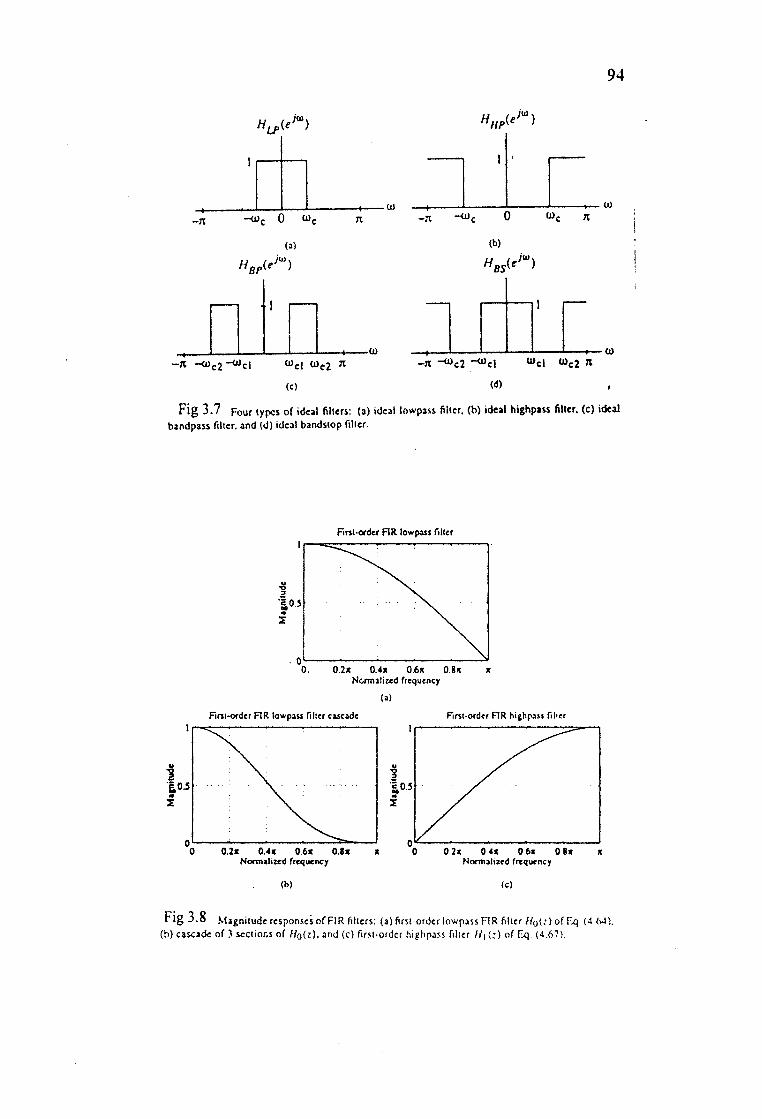
interest is the development of a realizable approximation to a given magnitude response

specification. There are four basic types of filters, namely, ideal lowpass filter, ideal highpass filter,

ideal bandpass filter and ideal bandstop filter, whose magnitude responses are shown in Fig 3.7.

Since the impulse response corresponding to each of these are noncasual and of infinite length, these

ideal filters are not realizable One way to develop a realizable approximation to these filters would

be to truncate the impulse response The magnitude response of FIR lowpass filter obtained by

truncating the impulse response of the ideal lowpass filter does not have sharp transition from

passband to stopband but, rather, exhibits a gradual “roll-off’.

Thus, as in the case of the analog filter design problem, the magnitude response

specifications of a digital filter in the passband and in the stopband are given with some acceptable

tolerances. In addition, a transition band is specified between the passband and the stopband to

permit the magnitude to drop off smoothly. For example, the magnitude |G(e’“)| of a lowpass filter

may be given as shown if Fig 3.8. As indicated in the figure, in the passband defined by

0 < co < ©p, we require that the magnitude approximates unity with an error of ± 8P, i.e.,

1-5P< |G(e®j)| < 1+8P, for |©| <©p (3.76)

In the stopband, defined by s , we require the magnitude approximate zero with an error of s, i.e.,

|G(e"j)| < 5, for to, <|to| < n (3.77)

The frequencies cop and to, are respectively, called the passband edge frequenc> and the

stopband edge frequency. The limits of the tolerances in the passband and stopband, 6P and 8, are

usually called the peak ripple values. Note that the frequency response G(e“j) of a digital filter is a

penodic function of to, and the magnitude response of a real coefficient digital filter is an even

function of to. Asa result, the digital filter specifications are given only for the range 0 < | coj < jr.

Often, the specifications of the digital filter are given in terms of the loss function,

<^(to) = - 201ogl 0[G(ejo5)|, in dB. Here the peak passband ripple ctp and the minimum stopband

attenuation as are given in dB, i.e., the loss specifications of a digital filter are given by

93

otp = -201ogl0(l- 8P) dB, (3.78)

a, = -201ogl 0(8,) dB. (3.79)

As in the case of an analog lowpass filter, the specifications for a digital lowpass filter may

alternatively be given in terms of its magnitude response, as in Fig 3.8a. Here the maximum value

of the magnitude in the passband is assumed to be unity, and the maximum passband de\ iation,

denoted as l / V(l+e2), is given by the maximum value of the magnitude in the passband. The

maximum stopband magnitude is given by 1/A.

For the normalized specification, the maximum value of the gain function or the minimum

value of the loss function is therefore 0 dB. The quantity ow given by

ow = 20!ogl 0(V(1 +s2)) dB (3.80)

is called the maximum attenuation. For 8P « 1, as is typically the case, it can be shown that

cw -201ogl 0(1-2 8„) = 2cxp (3.81)

The passband and stopband frequencies, in most applications, are specified in Hz, along with

the sampling rate of the digital filter. Since all filter design techniques are developed in terms of

normalized angular frequencies cop and Co* the specified critical frequencies need to be normalized

first before a specific filter design algorithm can be applied. Let Ft denote the sampling frequency

in Hz, and Fp and Fs denote, respectively, the passband and stopband edge frequencies in Hz. Then

the normalized angular edge frequencies in radians are given by

cop = Op = 2tiFd= 2 7iFDT (3.82)Ft Ft

©s = n_, = 2tcF, = 2ji F.T (3.83)Ft Ft

3.4.3 Selection of the Filter Type:

The second issue of interest is the selection of the digital filter type, i.e., whether an OR or an

FIR digital filter is to be employed. There are several advantages to using an FIR filter, since it can

94

,-------------

-cuc 0 wc n

(a)hbp^)

(c)

H (e}U>)nHPKe ’

1

-n —tuc 0 wc ji

(b)H8Sicim)

<d)

Fig 3.7 Four types of ideal filters: (a) ideal towpass filter, (b) ideal highpass filter, (c) ideal bandpass filler, and (d) ideal bandstop filter.

First-order FIR lowpass filler

(a)First-order RR lowpass filler cascade First-order RR highpass filler

(b) (c)

Fig 3.8 Magnitude responses of FIR filters: (a) first-order lowpass RR filter HqU) of F^j (4. (>4), (b) cascade of 3 sections of //q(;), and (c) first-order highpass filter //({;) of Eq (4.67>

95

be designed with exact linear phase and the filter structure is always stable with quantized filter

coefficients. However, in most cases, the order NFIR of an FIR filter is considerably higher than the

order NIIR of an equivalent IIR filter meeting the same magnitude specifications. In general, the

implementation of the FIR filter requires approximately NFIR multiplications per output sample,

where as the HR filter requires 2NHR+1 multiplications per output sample. In the form case, if the

FIR filter is designed with the linear phase, then the number of multiplications per output sample

reduces to approximately (NFIR+iy2. Likewise, most IIR filter design result in transfer functions

with zeros on the unit circle, and the cascade realization of an IIR filter order NIIR- with zeros on

the unit circle requires [(3NIIR+3)/2] multiplications per output sample. It has been shown by

Rabiner and Gold[l 3] that for most practical filter specifications, the ratio NFIR/NIIR is typically of

the order of tens or more, and as a result, the IIR filter usually is computationally more efficient.

However, if the group delay of the OR filter is equalized by cascading it with an allpass equalizer,

then the savings in the computation may no longer be that significant^ 3], In many applications, the

linearity of the phase response of the digital filter is not an issue, making the HR filter preferable

because of the lower computational requirements.

3 .4 4 Basic Approaches to Digital Filter Design:

In the case of an IIR filter design, the most common practice is to convert the digital filter

specifications to analog lowpass prototype filter specifications, to determine the analog lowpass

filter transfer function Ha(s) meeting these specifications, and then to transform it into the desired

digital filter function G(z). This approach has been widely used for many reasons:

(a) Analog approximation techniques are highly advanced

(b) They usually yield closed-form solutions

(c) Extensive tables are available for analog filter design

(d) Many applications require the digital simulation of analog filters.

In the sequel, we denote an analog transfer function as

Ha(s) = Pa(s) (3,84)Da(s)

96

where the subscript “a” specifically indicates the analog domain. The digital transfer function

derived from Ha(s) is denoted by

G(z) = _P(z) (3.85)D(z)

The basic idea behind the conversion of an analog prototype transfer function Ha(s) to a

digital HR transfer function G(z) is to apply a mapping from s-domain to the z-domain so that the

essential properties of the analog frequency response are preserved. This implies that the mapping

function should be such that:

(a) The imaginary (j) axis in the s-plane be mapped onto the unit circle of the z-plane

(b) A stable analog transfer function be transformed into a stable digital transfer

function.

Unlike the HR digital filter design, the FIR filter design does not have any connection with the

design of analog filters. The design of FIR filters is therefore based on a direct approximation of the

specified magnitude response, with the often added requirement that the phase response be linear. A

casual FIR transfer function H(z) of length N is a polynomial in z-1 of degree N-l:,

N-l

H(z) = Z hlnlz-” (3.86)n=0

The corresponding frequency response is given by

N-l

H(e’“) = Z h|nle>n (3,87)nO

It is the fact that any finite duration sequence x[n] of length N is completely characterized by N

samples of its Fourier transform X(e’tfl). As a result, the design of an FIR filter of length N may be

accomplished by finding either the impulse response sequence {h[n}} or N samples of its frequency

response H(e*“). Also, to ensure a linear phase design, the condition hfN-l-n] = h[n] or -h[n] must

be satisfied. Two direct approaches to the design of FIR filters are the truncated Fourier series

approach and the frequency sampling approach.

REFERENCES OF CHAPTER 3:

1. John G Proakis and Dimitris G Manolakis, “Digital Signal Processing - Principles, Algorithms, and Applications”, Prentice Hall of India, New Delhi(1997).

2. Blahut RE, “Fast Algorithms for Digital Signal Processing”, Addison-Wesley, Reading(l 985).

3. Bluestein LI, “A Linear Filtering Approach to Computation of the Discrete Fourier Transform”, IEEE Trans Audio and Electroacoustics, 18, pp451-455(1970).

4. Brigham EO, “The Fast Fourier Transform and its Applications”, Prentice Hall,Englewood(l 988).

5. Bracewell RN, “The Fourier Transform and its Applications”, McGraw Hill, New York(l 978).

6. Childers DG (ed),’Modem Spectrum Analysis”, IEEE Press, New York(l978).

7. Crochiere RE and Rabinee IR, “Multirate Digital Signal Processing”, Prentice & Hall, EC( 1983).

8. Cooley JW, Lewis P and Eelch P.D,’’The Fast Fourier Transform and its Applications’, IEE Trans Education, 12, pp27-34(1969).

9. Constantinides AG,’’Spectral Transformation for Digital Filters”, Pro IEEE, 117, pi 585- 1590(1979).

10. Brown JL(Jr),’’First Order Sampling of Bandpass Signals-A New Approach”, IEEE Trans Information Theory, 26, pp613-615(1980).

11. Bomar BW, “New Second-Order State-Space Structures for Realizing Low Roundoff Noise Digital Filters”, IEEE Trans Acoustics, Speech and Signal Processing, 33, ppl06-110(1985).

12. Price R, “Mirror FFT and Phase FFT Algoriths”, Raytheon Research Div (1990).

13. L.R.Rabiner and B.Gold, “Theory and Application of Digital Signal Processing”, Prentice-

Hall, Englewood Cliffs NJ, 1075.