3F1 Information Theory Course - University of Cambridge

3F1 Information Theory Course (supervisor copy) 1

3F1 Information Theory Course

Nick Kingsbury

October 17, 2012

Contents

1 Introduction to Information Theory 4

1.1 Source Coding . . . . . . . . . . . . . . . . . . . . . . . . . . . . . . . . . . . . . 4

1.2 Variable length codes . . . . . . . . . . . . . . . . . . . . . . . . . . . . . . . . . 5

1.3 Instantaneous Codes . . . . . . . . . . . . . . . . . . . . . . . . . . . . . . . . . 6

1.4 Average Code Length . . . . . . . . . . . . . . . . . . . . . . . . . . . . . . . . . 7

1.5 Source Entropy . . . . . . . . . . . . . . . . . . . . . . . . . . . . . . . . . . . . 8

1.6 Properties of the source entropy . . . . . . . . . . . . . . . . . . . . . . . . . . . 10

1.7 Information rate and redundancy . . . . . . . . . . . . . . . . . . . . . . . . . . 13

2 Good Variable-Length Codes 15

2.1 Expected Code Length . . . . . . . . . . . . . . . . . . . . . . . . . . . . . . . . 15

2.2 Kraft Inequality . . . . . . . . . . . . . . . . . . . . . . . . . . . . . . . . . . . . 16

2.3 Bounds on Codeword Length . . . . . . . . . . . . . . . . . . . . . . . . . . . . 17

2.4 Shannon Fano Coding . . . . . . . . . . . . . . . . . . . . . . . . . . . . . . . . 18

2.5 Huffman Coding . . . . . . . . . . . . . . . . . . . . . . . . . . . . . . . . . . . 20

2.6 Extension Coding . . . . . . . . . . . . . . . . . . . . . . . . . . . . . . . . . . . 22

2.7 Arithmetic Coding . . . . . . . . . . . . . . . . . . . . . . . . . . . . . . . . . . 24

3 Higher Order Sources 27

3.1 Higher order sources . . . . . . . . . . . . . . . . . . . . . . . . . . . . . . . . . 27

3.2 Non-independent variables . . . . . . . . . . . . . . . . . . . . . . . . . . . . . . 28

2 3F1 Information Theory Course (supervisor copy)

3.3 Mutual Information . . . . . . . . . . . . . . . . . . . . . . . . . . . . . . . . . . 29

3.4 Algebra of Mutual Information . . . . . . . . . . . . . . . . . . . . . . . . . . . 30

3.5 Example: the Binary Symmetric Communications Channel . . . . . . . . . . . . 30

3.6 Markov sources . . . . . . . . . . . . . . . . . . . . . . . . . . . . . . . . . . . . 31

3.7 Coding a first order source . . . . . . . . . . . . . . . . . . . . . . . . . . . . . . 34

3.8 Example: Lossless Image Coding . . . . . . . . . . . . . . . . . . . . . . . . . . 35

4 Sources with Continuous Variables 39

4.1 Entropy of continuous sources . . . . . . . . . . . . . . . . . . . . . . . . . . . . 39

4.2 Entropy change due to quantisation . . . . . . . . . . . . . . . . . . . . . . . . . 41

4.3 Mutual information of continuous variables . . . . . . . . . . . . . . . . . . . . . 43

4.4 Example: the Gaussian Communications Channel . . . . . . . . . . . . . . . . . 43

3F1 Information Theory Course (supervisor copy) 3

Pre-requisites

This course assumes familiarity with the following Part IB courses:

• Probability (Paper 7);

• Signal and Data Analysis (Paper 6);

Book / Paper List

• T. M. Cover and J. A. Thomas, ‘Elements of Information Theory’, 2nd ed.(Wiley, 2006).

A very good and comprehensive coverage of all the main aspects of Information Theory.Very clearly written.

• D. J. C. MacKay, ‘Information Theory, Inference, and Learning Algorithms’(CUP, 2003).

This book explores the whole topic of Information Theory in a very approachable form.It goes well beyond exam requirements in 3F1, but will be very useful for those interestedin a broader understanding of the subject. The book is downloadable FREE in pdf (11MB) from:

http://www.inference.phy.cam.ac.uk/mackay/itila/book.html

This version should not be printed. A printed version is produced by CU Press, and costsabout £35.

• C. E. Shannon, ‘A Mathematical Theory of Communication’,in The Bell System Technical Journal, Vol. 27, pp. 379-423, 623-656, July & October,1948.

A reprinted version is downloadable FREE in pdf (0.4 MB) from:

http://cm.bell-labs.com/cm/ms/what/shannonday/shannon1948.pdf

Acknowledgement

This course is developed from an earlier course on Information Theory, given by Dr TomDrummond until December 2004. I would like to thank him very much for allowing me to basemuch of this course on his lecture notes and examples. I am also grateful to Dr Albert Guilleni Fabregas, who has provided valuable comments on the communications related aspects of thecourse.

Nick Kingsbury.

4 3F1 Information Theory Course - Section 1 (supervisor copy)

1 Introduction to Information Theory

Information theory is concerned with many things. It was originally developed for designingcodes for transmission of digital signals (Shannon, late 1940s).

Other applications include:

• Data compression (e.g. audio using MP3 and images using JPEG)

• Signal analysis

• Machine learning

We will begin by looking at the transmission of digital data over the internet and othernetworks, and its storage in computers and on other media. The aim is to maximise throughputof error-free data and minimise file sizes.

1.1 Source Coding

This is concerned with the representation of messages as digital codes.

The aim is to make messages take up the smallest possible space.

A famous example for plain english text is:

A •− J • − −− S • • •B − • • • K − • − T −C − • −• L • − • • U • • −D − • • M −− V • • •−E • N −• W • − −F • • −• O −−− X − • •−G −− • P • − −• Y − • −−H • • • • Q −− •− Z −− ••I • • R • − •

This is Morse Code (from about 1830) and has some interesting properties:

• The codes are not all the same length

• The code uses two symbols ... (or does it?)

How do you decode this?

• • • • • • − • • • − • • − −− • − −−−− • − • • − • • − • •

The duration of the space between symbols in morse is very important as it allows us todistinguish 3 E’s from an S, for example.

3F1 Information Theory Course - Section 1 (supervisor copy) 5

1.2 Variable length codes

If we want to transmit information as quickly as possible, it is useful to use codes of varyinglengths if the source generates symbols with varying probabilities.

We can use shorter codes for common symbols and longer codes for rare ones.

e.g. in Morse code E = •, whereas Q = −− •− .

From now on we shall consider only binary codes – i.e. codes using only 0 and 1 to form theircodewords.

Constraints:

1. There must be no ambiguity in the code

(so for binary codes, “0” and “00” cannot both be codewords).

2. It must be possible to recognise a codeword as soon as the last bit arrives

(so “0” and “01” cannot both be codewords).

A code which satisfies these two conditions is called an Instantaneous Code.

Examples

A source emits a sequence of symbols from the set {A, B, C, D}

Two different codes for transmitting these symbols are proposed:

Code 1 Code 2

A 00 0B 01 10C 10 110D 11 111

Which of these codes is better?

If all 4 symbols are equally likely, then Code 1 is best:

• Average word length of Code 1 =2 + 2 + 2 + 2

4= 2 bits.

• Average word length of Code 2 =1 + 2 + 3 + 3

4= 2.25 bits.

BUT if symbol A is more likely than B, and B is more likely than C or D, then the averageword length of Code 2 reduces, while that of Code 1 stays the same.


1.3 Instantaneous Codes

An alternative way to phrase the constraints is to state the Prefix Condition:

No codeword may be the prefix of any other codeword

(A prefix of a codeword means a consecutive sequence of digits starting at the beginning)

This condition allows us to represent (and decode) the code using a tree:

B

?

A

?

?

C

D

ABCD

0

110111

10

Finite state machine

Labelling the upper output of each query node as 0 and the lower output as 1 corresponds tothe code words on the left.

This diagram represents a finite state machine for decoding the code.


1.4 Average Code Length

An important property of a code is the average length L of the codewords (averaged according

to the probabilities). For N symbols with probabilities pi and codeword lengths li bits, L is

given by the expectation of the lengths:

L = E[ li ] =N∑i=1

pi li bits

Example

Consider the two codes given in the example above.

If the symbol probabilities and codeword lengths are given by:

pi Code 1 li Code 2 liA 0.6 2 1B 0.2 2 2C 0.1 2 3D 0.1 2 3

Average word length for Code 1 is:

0.6× 2 + 0.2× 2 + 0.1× 2 + 0.1× 2 = 1.2 + 0.4 + 0.2 + 0.2 = 2 bits

Average word length for Code 2 is:

0.6× 1 + 0.2× 2 + 0.1× 3 + 0.1× 3 = 0.6 + 0.4 + 0.3 + 0.3 = 1.6 bits


1.5 Source Entropy

We need a mathematical foundation for choosing efficient codes. This requires a way of mea-suring:

1. Information content of a Source

2. Information content of each symbol

3. Efficiency of a code

Shannon (1948) had a basic insight:

The information content of a message depends on its a priori probability

• You winning the national lottery – rare, so lots of information.

• A typical party political broadcast – predictable, so not much information.

The most information is associated with rare events.

Consider an order-0 process (also called a memoryless process), in which a source S selectseach symbol i with probability Pi (i = 1..N).

C 0.2ADDBDACADC...

D

B

A 0.3

0.1

0.4

S:

We want a measure of the average information per symbol H(S).

What properties should H(S) have?

1. It should be continuous in the probabilities pi.

2. If the pi are equal then H(S) should increase with N

3. If S1 and S2 are two independentmessage sources then a combined source(S1, S2) should have

H(S1, S2) = H(S1) +H(S2)

(i.e. the information obtained by combining two independent message sources is the sum

of the information from each source – e.g. an 8-bit message can be regarded as the sum

of two 4-bit messages).


We now show that these properties are satisfied if H(S) is of the form:

H(S) = −K

N∑i=1

pi log(pi) where K > 0

Shannon called H(S) the information entropy because of its similarity to the concept ofentropy in statistical mechanics, where pi represents the probability of being in a particularthermal microstate i (as in Boltzmann’s H-theorem).

Considering the above 3 properties in turn, using H(S) defined above:

1. pi log(pi) is continuous for each pi in the range 0 ≤ pi ≤ 1,so H(S) will also be continuous in the pi. (Note: p log(p) = 0, when p = 0.)

2. If the pi are equal, then pi =1

N. Hence

H(S) = −KN∑i=1

1N log( 1

N ) = KN∑i=1

1N log(N) = K log(N)

If H(S) is to increase with N , then K must be positive.

3. Let S1 and S2 be sources with N1 and N2 symbols respectively, and with probabilities

p1 . . . pN1 and q1 . . . qN2 . Hence

N1∑i=1

pi = 1 and

N2∑j=1

qj = 1

Entropies of S1 and S2 are then

H(S1) = −K

N1∑i=1

pi log(pi) and H(S2) = −K

N2∑j=1

qj log(qj)

and the combined source (S1, S2) will have N1N2 states with probabilities piqj, so

H(S1, S2) = −K

N1∑i=1

N2∑j=1

piqj log(piqj)

= −K

N1∑i=1

N2∑j=1

piqj[log(pi) + log(qj)]

= −K

N1∑i=1

pi log(pi)

N2∑j=1

qj −K

N2∑j=1

qj log(qj)

N1∑i=1

pi

= −K

N1∑i=1

pi log(pi)−K

N2∑j=1

qj log(qj)

= H(S1) +H(S2) as required.


The key to this final result lies in the relationship

log(piqj) = log(pi) + log(qj)

which shows why the entropy expression must contain a log(p) term and not any othernon-linear function.

In appendix 2 on p. 28 of Shannon’s 1948 paper (see book/paper list), he proves that the abovelogarithmic form for H(S) is the only form which satisfies the above 3 properties.

1.6 Properties of the source entropy

H(S) = −KN∑i=1

pi log(pi)

The choice of K is arbitrary (as long as it is positive) and equates to choosing a base for the

logarithm. The convention is to to use base 2 logs and choose K = 1, so that

H(S) = −N∑i=1

pi log2(pi)

The unit of entropy is then bits.

This is equivalent to using natural logs (base e) and choosing K =1

ln(2), so that

H(S) = − 1

ln(2)

N∑i=1

pi ln(pi)

For a source with N = 2n equiprobable states, the entropy is log2 N = n bits, which is theword-length for a simple uniform-length binary code for this source.

Reminder about logs:

Let y = 2x = (eln(2))x = ex ln(2)

Take base 2 and base e logs: x = log2(y) and x ln(2) = ln(y)

Therefore log2(y) =ln(y)

ln(2)

This works for any bases a and b, not just for 2 and e.


Examples:

1. Two symbols with probability 0.5 (coin flip):

H(S) = − 0.5 log2(0.5)− 0.5 log2(0.5) = log2(2) = 1 bit

2. Four symbols with probability 0.25:

H(S) = − 0.25 log2(0.25)× 4 = log2(4) = 2 bits

3. The roll of a 6-sided (fair) die:

H(S) = − 16 log2(

16)× 6 = log2(6) = 2.585 bits

4. Four symbols with probabilities 0.6, 0.2, 0.1 and 0.1 (the earlier example code):

H(S) = − 0.6 log2(0.6)− 0.2 log2(0.2)− 0.1 log2(0.1)− 0.1 log2(0.1)

= 0.4422 + 0.4644 + 0.3322 + 0.3322 = 1.5710 bits.

5. Two independent sources:

Symbol Probability pi −pi log2 pi

Source S1 A 0.7 0.3602B 0.3 0.5211

Source S2 α 0.5 0.5β 0.5 0.5

Entropies:

H(S1) = 0.3602 + 0.5211 = 0.8813 bit H(S2) = 0.5 + 0.5 = 1 bit

Symbol Probability −pi log2 pi

Source S Aα 0.35 0.5301= (S1, S2) Aβ 0.35 0.5301

Bα 0.15 0.4105Bβ 0.15 0.4105

Joint entropy:

H(S) = 0.5301 + 0.5301 + 0.4105 + 0.4105 = 1.8813 bits

which shows that:

H(S) = H(S1) +H(S2)


Properties of the source entropy (cont.)

Note that the entropy takes the form of an expectation:

H(S) = −N∑i=1

pi log2(pi) = E(− log2(pi))

So the information associated with each symbol is − log2(pi)

The entropy is maximised when all symbols are equiprobable.

For a source with two symbols with probabilities p and (1− p):

H(S) = − [ p log2(p) + (1− p) log2(1− p) ]

as shown below.

0

0.1

0.2

0.3

0.4

0.5

0.6

0.7

0.8

0.9

1

0 0.1 0.2 0.3 0.4 0.5 0.6 0.7 0.8 0.9 1

In general we may prove that for a code with N symbols, the entropy achieves a maximumvalue of log2 N when all the probabilities equal 1

N.

To do this we calculate

H(S)− log2N = −N∑i=1

pi(log2 pi + log2N) =N∑i=1

pi log2(1

Npi)

Then we use the relations:

log2 x =lnx

ln 2and ln x ≤ x− 1 (prove by simple calculus)

to show that H(S)− log2N ≤ 0, with the equality occurring when Npi = 1 for all pi.

Completion of this proof is examples sheet question 1. Note, we could, as an alternative, usecalculus directly on the pi terms, but this is not so easy because the pi must sum to unity atall times so they can’t be varied independently.


Plot of y = ln(x) and y = x− 1

-3

-2

-1

0

1

2

3

0 0.5 1 1.5 2 2.5 3 3.5 4

1.7 Information rate and redundancy

A source S uses an alphabet of N symbols, has entropy HS bit/symbol and produces f symbolsper second.

The information rate of the source is f HS bit/sec.

As discussed above, the maximum entropy an N -ary source can have is

Hmax = − log2(1N ) = log2N bit/symbol

The redundancy of the source is defined as (Hmax −HS) bit/symbol.


2 Good Variable-Length Codes

2.1 Expected Code Length

Recall from section 1.4 that the average codeword length is L =N∑i=1

pili bits.

To maximise message throughput on a channel with a given bit rate, we want to minimise L.

We will find out that L ≥ H(S) .

So we can define the Rate Efficiency as η = H(S)/L .

Examples:

1. Two equiprobable symbols with code 0 and 1:

p0 = p1 = 0.5 l0 = l1 = 1 bit

H(S) = 0.5× 1 + 0.5× 1 = 1 bit

L = 0.5× 1 + 0.5× 1 = 1 bit

η = 1

2. Four symbols with probabilities and two codes given in the table below

Symbol Probability Code 1 Code 2

A 0.125 00 000B 0.125 01 001C 0.25 10 01D 0.5 11 1

Probabilities are the same for both codes so H(S) is the same.

H(S) = 0.125× 3 + 0.125× 3 + 0.25× 2 + 0.5× 1 = 1.75 bits

L1 = 0.125× 2 + 0.125× 2 + 0.25× 2 + 0.5× 2 = 2 bits

η1 = 1.75/2 = 0.875

L2 = 0.125× 3 + 0.125× 3 + 0.25× 2 + 0.5× 1 = 1.75 bits

η2 = 1.75/1.75 = 1.0


2.2 Kraft Inequality

The Kraft inequality for a valid code with codeword lengths li, i = 1 . . . N , which satisfies the

prefix condition, states thatN∑i=1

2−li ≤ 1

For example consider code 2 from example above:

Symbol Code li 2−li

A 000 3 0.125B 001 3 0.125C 01 2 0.25D 1 1 0.5

Proof

Let m = maximum codeword length.

Consider the 2m possible words of length m

Assign each one to the codeword that is its prefix (if it has one).

There can be at most one codeword which is the prefix of any word of length m since if therewere two codewords which were both prefixes then the shorter one would be a prefix for thelonger one.

A codeword of length l is the prefix of 2m−l words of length m since there are m − l free bitsafter the codeword.

2m words codeword (prefix) li

000 000 3001 001 3

010011

}01 2

100101110111

1 1

m bits

X X X ? ?

of codeword bits

l bits m−l free

So for the example above, m = 3. The codeword 01 has length 2 and is the prefix for23−2 = 21 = 2 words of length 3 (namely 010 and 011).

Adding up the words of length m assigned to each codeword gives:

N∑i=1

2m−li ≤ 2m HenceN∑i=1

2−li ≤ 1


The Kraft inequality is a sufficient condition as well as a necessary one. So if you have a setof lengths that satisfy the inequality, then a set of codewords with those lengths exists. Thecodewords can easily be generated using the same trick as in the proof:

Find the longest codeword, make a list of all words of that length in ascending (ordescending) binary order. Taking the code lengths in ascending order, assign 2m−li

words to each code and record the common prefix (of length li) as the codeword.

2.3 Bounds on Codeword Length

We will show that a code can be found such that

H(S) ≤ L < H(S) + 1

This states two things. First that the average codeword length must be at least the entropy ofthe source. Second that it is possible to find a code for which the average codeword length isless than 1 bit more than the entropy.

Tackling the LHS of the inequality first, consider H(S)− L

H(S)− L =∑i

−pi log2(pi)−∑i

pili =∑i

pi

(log2(

1

pi)− li

)=∑i

pi log2(2−li

pi) =

1

ln(2)

∑i

pi ln(2−li

pi)

≤ 1

ln(2)

∑i

pi

(2−li

pi− 1

)since ln(x) ≤ x− 1

=1

ln(2)

(∑i

2−li −∑i

pi

)≤ 0 (Kraft inequality)

Note that if pi = 2−li then H(S) = L since we can substitute log2(1) into the 2nd line above.


2.4 Shannon Fano Coding

We can show the RHS inequality of the codelength bound by designing a code that will alwayssatisfy it.

First we choose integer codelengths li such that

li = ⌈ log2(1

pi)⌉

This means that

log2(1

pi) ≤ li < log2(

1

pi) + 1

The LHS of this says 2−li ≤ pi, and, since∑

pi ≤ 1, we obey the Kraft inequality. So a codeexists (we’ll actually generate the code in a minute).

Multiplying the RHS by pi and summing to get L gives

L =∑i

pili <∑i

pi

(log2(

1

pi) + 1

)= H(S) + 1

So this choice of codelengths will do it, but how do we actually produce a code?

Shannon’s original scheme (invented independently by Fano) worked as follows:

1. Sort the probabilities into descending order;

2. Make a cumulative probability table (adding each probability to all those above it);

3. Expand the cumulative probabilities as a binary fraction;

4. Take the first li digits in the binary fraction as the code.

For example, consider a source that produces six symbols with probabilities 0.34, 0.19, 0.17,0.1, 0.1, 0.1.

Symbol pi li∑

pi−1 binary S-F code Better code

A 0.34 2 0 0.000000 00 00B 0.19 3 0.34 0.010101 010 01C 0.17 3 0.53 0.100001 100 100D 0.1 4 0.7 0.101100 1011 101E 0.1 4 0.8 0.110011 1100 110F 0.1 4 0.9 0.111001 1110 111

This Shannon-Fano (S-F) code wastes some of the codespace - by inspection we see thatthe codes 011, 1010, 1101 and 1111 could be added without violating the prefix condition.Alternatively they can be combined with existing codewords to shorten them and give thebetter (more efficient) code in the final column. To do this, 011 was combined with 010 togenerate the shorter code 01, and then 1010 with 1011 to give 101, etc.


How did Shannon know that the S-F algorithm would always generate a valid code?

Well the codes get longer, so he only had to make sure that each code was not a prefix ofany that followed it. But the choice of codelength ensures that we add at least 1 to the leastsignificant bit of the code. For example the probability of C is more than 2−3 so we know thatthe first three ‘decimal’ (actually binary) places of the cumulative probability for D must beat least 0.100 + 0.001 = 0.101, so C cannot be a prefix for D (or anything that follows).

In the above example the entropy of the source is 2.4156 bits.

The average length of the S-F code in the table is

LSF = 0.34× 2 + 0.19× 3 + 0.17× 3 + 0.1× 4× 3 = 2.96 bits

This still satisfies the bound that it should be no more than 1 bit worse than the entropy.

However the ‘better’ code gets much closer with an average length of

Lbetter = 0.34× 2 + 0.19× 2 + 0.17× 3 + 0.1× 3× 3 = 2.47 bits

We can see quickly that the S-F code is not likely to be very good because, for this code∑i

2−li = 0.25 + 2× 0.125 + 3× 0.0625 = 0.6875

which is a lot less than the permitted Kraft upper limit of unity. Hence we are only usingabout 69% of the available code space.

The ‘better’ code in this case equals the Kraft upper limit and uses 100% of the code space,because we have combined all unused regions of code space with used codewords in order toshorten them without violating the prefix condition.


2.5 Huffman Coding

The Shannon Fano algorithm creates reasonably efficient codes, but we have seen the codeis still wasteful. There exists an optimal algorithm (that guarantees to minimise the averagecodeword length and use 100% of the codespace) called the Huffman coding algorithm, asfollows.

Given symbols {x1 . . . xN} with probabilities {p1 . . . pN}:

1. Make a list of symbols with their probabilities (in descending order helps).

2. Find the two symbols in the list with the smallest probabilities and create a new nodeby joining them. Label the two new branches with 0 and 1 using some predefined rule(e.g. upper branch = 0).

3. Treat the new node as a single symbol with probability equal to the sum of the two joinedsymbols (which it now replaces in the list).

4. Repeat from step 2 until the root node is created with probability = 1.0 .

5. Generate the codewords for each symbol, by starting from the root node and followingthe branches of the tree until each symbol is reached, accumulating the binary labelsfrom step 2 to form each codeword in turn (root node symbol is first, i.e. on the left).

Using the same 6-symbol source as before, figs. 2.1 to 2.3 show the development of a Huffmancode tree using this algorithm, after one, three and all iterations respectively. Note the code-words in fig. 2.3, derived in step 5 of the algorithm after the final (5th) iteration of steps 2 to4. These codewords have the same lengths as the ‘better’ code in the above table and hencewill give the same average length of 2.47 bits.

Symbols

A

B

C

D

E

F

Probabilities

0.34

0.19

0.17

0.1

0.1

0.1

s0

1 0.2

Codes

Fig 2.1: Huffman code tree - after node 1.


Symbols

A

B

C

D

E

F

Probabilities

0.34

0.19

0.17

0.1

0.1

0.1

s0

1 0.2

s0

1 0.27

s

0

1

0.39

Codes

Fig 2.2: Huffman code tree - after nodes 1 to 3.

Symbols

A

B

C

D

E

F

Probabilities

0.34

0.19

0.17

0.1

0.1

0.1

s0

1 0.2

s0

1 0.27

s

0

1

0.39

s0

1

0.61

�� s0

1

1.0

Root

Codes

00

10

010

011

110

111

Fig 2.3: Huffman code tree - completed, with codewords.


2.6 Extension Coding

The efficiency of a code is defined as η = H(S)/L.

Recall that H(S) ≤ L < H(S) + 1 .

This inequality tells us that

1 ≥ η >H(S)

H(S) + 1

If H(S) << 1 then η can be very small.

E.g. for a source with two symbols and probabilities 0.999 and 0.001, H(S) = 0.011 but wehave to use 1 bit per symbol so η is only 1.1% .

Huffman codes are usually very efficient (η ∼ 95 to 99%) but if one of the pi is significantlygreater than 0.5, the code can become inefficient, especially if the pi approaches unity.

A solution to this problem is to group sequences of symbols together in strings of length K.This is called extending the source to order K. If we have an alphabet of N symbols inthe original source, we will then have an alphabet of NK symbols in the extended source.

If the source is memoryless then the probability of a given combined symbol in the extendedsource is just the product of the probabilities of each symbol from the original source thatoccurs in the combination.

The entropy of the extended source is then simply

K ×H(S)

So η is bounded below by

η >KH(S)

KH(S) + 1

which tends to 1 for large K. In practice K only needs to be large enough to bring theprobability of the most common extended symbol down to approximately 0.5 .

Example

Sym

A

B

C

Probs.

0.75

0.2

0.05

s0

1 0.25

s0

1

1.0

Codes

0

10

11

Fig 2.4: Huffman code for 3-symbol source with one very likely symbol.


Sym

AA

AB

BA

BB

AC

CA

BC

CB

CC

Probs.

0.5625

0.15

0.15

0.04

0.0375

0.0375

0.01

0.01

0.0025

s0

1 0.0125

s0

1

0.0225

s0

1

0.06

s0

1

0.0775

s0

1

0.1375

s0

1

0.2875

s0

1

0.4375

s0

1

1.0

Codes

0

10

110

11100

11101

11110

111110

1111110

1111111

Fig 2.5: Huffman code for order-2 extended source with 32 = 9 symbols.

The 3-symbol source in fig. 2.4 can be analysed as follows:

H(S) = −[ 0.75 log2(0.75) + 0.2 log2(0.2) + 0.05 log2(0.05) ]

= 0.9918 bits

LS = 0.75× 1 + 0.2× 2 + 0.05× 2 = 1.25 bits

ηS =0.9918

1.25= 79.34%

If we extend to order 2, as in fig. 2.5, the results become:

H(S, S) = 2H(S) = 1.9836 bits

LS,S = 0.5625× 1 + 0.15(2 + 3) + 0.04× 5 + 0.0375(5 + 5)

+ 0.01(6 + 7) + 0.0025× 7 = 2.035 bits

ηS,S =1.9836

2.035= 97.47%

Note the dramatic increase in efficiency with just order-2 extension!


2.7 Arithmetic Coding

Arithmetic Coding is an algorithm for extending the order to the entire length of the messageusing a form of Shannon-Fano coding. The inefficiencies of S-F coding become negligible whenthe order is large. This technique was invented and developed by several researchers (Elias,Rissanen and Pasco) at IBM in the early 1980s.

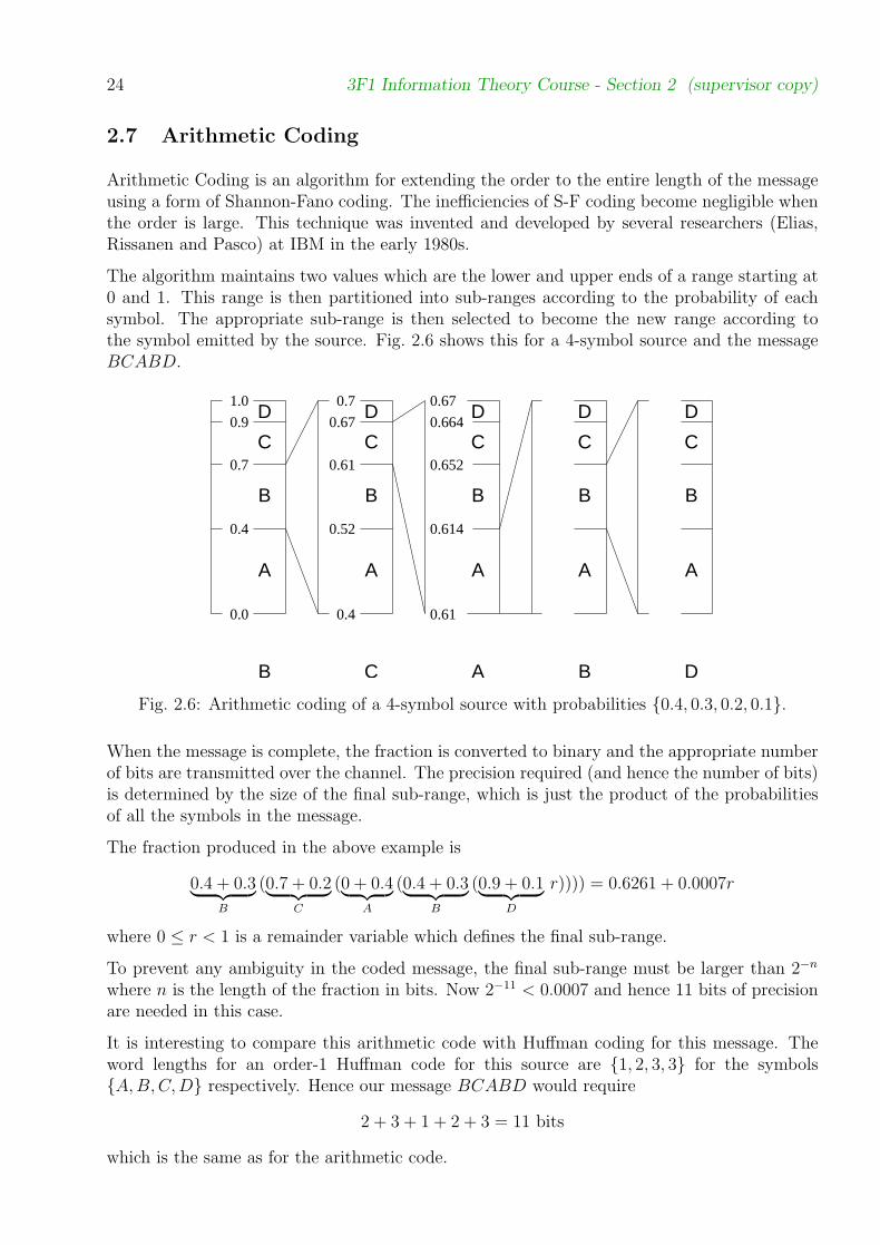
The algorithm maintains two values which are the lower and upper ends of a range starting at0 and 1. This range is then partitioned into sub-ranges according to the probability of eachsymbol. The appropriate sub-range is then selected to become the new range according tothe symbol emitted by the source. Fig. 2.6 shows this for a 4-symbol source and the messageBCABD.

B C A D

D

C

B

A

0.9

0.7

0.4

1.0

0.0

D

C

B

A

0.67

0.61

0.52

0.7

0.4

D

C

B

A

D

C

B

A

D

C

B

A

0.61

0.67

0.664

0.652

0.614

B

Fig. 2.6: Arithmetic coding of a 4-symbol source with probabilities {0.4, 0.3, 0.2, 0.1}.

When the message is complete, the fraction is converted to binary and the appropriate numberof bits are transmitted over the channel. The precision required (and hence the number of bits)is determined by the size of the final sub-range, which is just the product of the probabilitiesof all the symbols in the message.

The fraction produced in the above example is

0.4 + 0.3︸︷︷︸B

(0.7 + 0.2︸︷︷︸C

(0 + 0.4︸︷︷︸A

(0.4 + 0.3︸︷︷︸B

(0.9 + 0.1︸︷︷︸D

r)))) = 0.6261 + 0.0007r

where 0 ≤ r < 1 is a remainder variable which defines the final sub-range.

To prevent any ambiguity in the coded message, the final sub-range must be larger than 2−n

where n is the length of the fraction in bits. Now 2−11 < 0.0007 and hence 11 bits of precisionare needed in this case.

It is interesting to compare this arithmetic code with Huffman coding for this message. Theword lengths for an order-1 Huffman code for this source are {1, 2, 3, 3} for the symbols{A,B,C,D} respectively. Hence our message BCABD would require

2 + 3 + 1 + 2 + 3 = 11 bits

which is the same as for the arithmetic code.


We would need a much longer message to be able to see any significant difference between theperformance of the codes as they are both very efficient.

The main advantage of arithmetic codes is that they can easily be designed to adapt to changingstatistics of the symbols as the message progresses, and it is not necessary to know the symbolprobabilities before the coding starts. It is very difficult to do this with Huffman codes, whichmust be designed in advance.

For these reasons, arithmetic codes are now used extensively in JPEG-2000 image coders andin MPEG-4 (high-definition) video coders. Note that there are special scaling techniques thatcan be used in practice, to prevent arithmetic precision problems when the message is long andthe sub-ranges get very small indeed.

A lot more detail on arithmetic codes is given in chapter 6 of David MacKay’s online book.


3 Higher Order Sources

3.1 Higher order sources

Until now we have dealt with simple sources where the probabilities for successive symbols areindependent.

This is not true for many sources (e.g. English text).

If a “Q” appears in the signal, there is a high probability that the next symbol will be a “U”.So the “Q” is giving us information about the next symbol.

More generally, symbol n provides information about symbol n+ 1.

We should be able to exploit this to make a more efficient code.

Examples of English text

The following samples of text were generated by a random number generator, which pickedletters and spaces using the same probability distributions as occur in natural english. Theonly difference is that in the 1st, 2nd and 3rd-order cases, the probabilities of the current letterdepended on what letter or letters came before the one being picked.

0 order Markov model: (letters are independent)

OCRO HLI RGWR NMIELWIS EU LL NBNESEBYA TH EEI ALHENHTTPA OOBTTVANAH BRL

1st order Markov model: (each pdf is conditional on the previous letter)

ON IE ANTSOUTINYS ARE T INCTORE ST BE S DEAMY ACHIN D ILONASIVE TU-COOWE AT TEASONARE FUSO TIZIN ANDY TOBE SEACE CTISBE

2nd order Markov model: (each pdf is conditional on the two previous letters)

IN NO IST LAT WHEY CRATICT FROURE BERS GROCID PONDENOME OF DEMON-STRURES OF THE REPTAGIN IS REGOACTIONA OF CRE

3rd order Markov model: (each pdf is conditional on the three previous letters)

THE GENERATED JOB PROVIDUAL BETTER TRAND THE DISPLAYED CODE ABOVERYUPONDULTS WELL THE CODERST IN THESTICAL IT DO HOCK BOTHE MERG IN-STATES CONS ERATION NEVER ANY OF PUBLE AND TO THEORY EVENTIAL CAL-LEGAND TO ELAST BENERATED IN WITH PIES AS IS WITH THE

Note the dramatic increase in similarity to english in the higher order models.

To analyse these sort of effects, we need some information theory mathematics about non-independent random variables.


3.2 Non-independent variables

If two random variables X and Y are independent then for any given (x, y):

P (x, y) = P (x)P (y)

If the variables are not independent then P (x, y) can be arbitrary, so we must look at the jointprobability distribution P (X, Y ) of the combined variables. Here is an example:

P (X, Y ) :

X a b c∑

X

Y

α 0.3 0.02 0.01 0.33

β 0.02 0.3 0.02 0.34

γ 0.01 0.02 0.3 0.33∑Y 0.33 0.34 0.33 1.0

For X we can compute the probability that it takes the value a, b or c by summing theprobabilities in each column of the table. We can then compute the entropy of X:

H(X) = H([0.33 0.34 0.33]T ) = 1.5848 bits; and similarly for Y .

(For convenience I used the Matlab function entropy(p) given below.)

We can also compute the entropy of X given Y = α, β or γ:

H(X|α) = −∑

i p(xi|α) log2 p(xi|α)= H([0.3 0.02 0.01]T/0.33) = 0.5230 bits

H(X|β) = −∑

i p(xi|β) log2 p(xi|β)= H([0.02 0.3 0.02]T/0.34) = 0.6402 bits

H(X|γ) = −∑

i p(xi|γ) log2 p(xi|γ)= H([0.01 0.02 0.3]T/0.33) = 0.5230 bits

Clearly these are each a lot lower than H(X), and this is because there is high correlationbetween X and Y , as seen from the relatively large diagonal terms in the above 3 × 3 jointprobability matrix. So if we know Y , we can make a much better guess at X because it is verylikely to be the same as Y in this example.

We shall now look at this more formally.

function h = entropy(p)

% Calculate the entropies of processes defined by the columns of probability

% matrix p. The max function overcomes problems when any elements of p = 0.

%

h = -sum(p .* log(max(p,1e-10))) / log(2);

return;


3.3 Mutual Information

The average entropy of X given Y can be computed by adding up these three entropies mul-

tiplied by the probability that Y = α, β or γ :

H(X|Y ) = H(X|α) p(α) +H(X|β) p(β) +H(X|γ) p(γ)= 0.5230 . 0.33 + 0.6402 . 0.34 + 0.5230 . 0.33

= 0.5628 bits

This entropy is much less than H(X) which means that on average, the random variable Xcarries less information if you already know Y than if you don’t.

In other words, knowing Y provides some information about X. This mutual information

can be measured as the drop in entropy:

I(X;Y ) = H(X)−H(X|Y )

In this case it is 1.5848− 0.5628 = 1.0220 bits.

Based on the above arguments, we may obtain the following general expressions for conditional

entropy and mutual information:

H(X|Y ) = −∑j

p(yj)∑i

p(xi|yj) log2 p(xi|yj)

= −∑j

∑i

p(xi, yj) log2 p(xi|yj) since p(x, y) = p(x|y) p(y)

I(X;Y ) = −∑i

p(xi) log2 p(xi) +∑j

∑i

p(xi, yj) log2 p(xi|yj)

=∑j

∑i

p(xi, yj)[log2 p(xi|yj)− log2 p(xi)] since∑j

p(x, yj) = p(x)

=∑j

∑i

p(xi, yj) log2

(p(xi|yj)p(xi)

)

I(Y ;X) can also be obtained in the same way and, using Bayes rule, it turns out that:

I(Y ;X) = I(X;Y ) (see example sheet)

Hence X provides the same amount of information about Y as Y does about X; sothis is called the mutual information between X and Y .


3.4 Algebra of Mutual Information

We can also compute the entropy of the joint probability distribution

H(X,Y ) = −∑i

∑j

p(xi, yj) log2 p(xi, yj) = −∑i

∑j

pi,j log2(pi,j)

where the pi,j are the elements of matrix P (X, Y ).

In our example, H(X, Y ) = 2.1477 bits.

We find that

H(X, Y ) = H(X) +H(Y |X) = H(Y ) +H(X|Y )

= H(X) +H(Y )− I(X;Y )

In other words if I’m going to tell you the values of X and Y , I can tell you X first and Ysecond or vice versa. Either way, the total amount of information that I impart to you is thesame, and it is I(X;Y ) less than if the two values were told independently.

Note that this all applies even when P (X,Y ) is not a symmetric matrix and X and Y havedifferent probabilities. The only requirement on P (X,Y ) is that the sum of all its elementsshould be unity, so that it represents a valid set of probabilities.

3.5 Example: the Binary Symmetric Communications Channel

An important use of the Mutual Information concept is in the theory of digital communications.In section 2.2.1 of the 3F1 Random Processes course we considered the detection of binarysignals in noise and showed how the presence of additive noise leads to a probability of errorthat can be calculated from the signal-to-noise ratio of the channel.

Let the probability of error on a channel U be pe, and let the input and output of U be random

processes X and Y . U is called symmetric if pe is the same for both states of its input

X. The mutual information of U is then

I(Y ;X) = H(Y )−H(Y |X) = H(Y )−∑x

p(x) H(Y |X = x)

= H(Y )− [p(0) H([(1− pe) pe]) + p(1) H([pe (1− pe)])]

= H(Y )−H([pe (1− pe)]) = H(Y )−H(U)

Note that the probabilities of the output Y are given by

p(y) = (1− pe) p(X = y) + pe p(X ̸= y) for y = 0, 1

so if we know p(X), we can calculate p(Y ) and hence H(Y ).

The mutual information of U tells us how much information is passed through U from X to Y .


The Capacity CU of the channel U is defined (by Shannon) as the maximum of the mutual

information over all possible choices for p(X). In the case of the binary symmetric channel this

occurs when p(X) = [0.5 0.5], so that p(Y ) = [0.5 0.5] also and H(Y ) = 1. Hence

CU = maxp(X) I(Y ;X) = 1−H(U)

The capacity of a channel tells us the maximum number of bits of information pertransmitted symbol that we can expect to be able to pass through the channelerror-free, assuming that a very good error-correcting code is used. Hence thereciprocal of this tells us the minimum amount of redundancy (code rate) that is likely to beneeded in an error-correcting code for the channel.

For example if pe = 0.1, then H(U) = H([0.1 0.9]) = 0.469 (see graph on page 12 of thesenotes), and so CU = 0.531 bits per transmitted bit. Hence for every 1000 bits transmitted overthe noisy channel, only 531 bits of information can be reliably passed (assuming a good error-correcting code is available to convert the raw bit error rate of 1-in-10 down to essentially zeroerror probability). An (ideal) error correction code with a rate of at least 531 : 1000 = 1 : 1.884would therefore be required to transmit reliably over this channel. Typically a code rate ofapproximately 1 : 2 would be needed in practice, although some of the latest turbo or low-density parity check (LDPC) coding methods could get closer to theory than this.

These ideas can readily be extended to channels for non-binary sources and with non-symmetricerror probabilities. In fact, the example probability matrix P (X,Y ) in section 3.2 (page 28)could apply to a 3-level communication channel with unequal error probabilities and a slightlyunequal input distribution p(X).

3.6 Markov sources

An interesting and useful class of dependent random sources are those in which the probabilitydistribution for each new symbol (or state) in a stream depends only on a finite numberof previous symbols (states), and not on the whole stream of previous symbols. These areknow as Markov sources.

More formally we can define them as follows:

An N th-order Markov Source is a sequence of random variables S0, S1, S2, . . . , such thatthe probability distribution of Sn conditional on S0, . . . Sn−1 is a function of Sn−N , . . . Sn−1

only. (i.e. each Sn is conditional only on the most recent N samples.)

When N is small, this considerably simplifies the analysis of dependent sources, and it is oftenquite a good assumption to make in real systems.


Conditional probability tables

For a first-order Markov process, we usually represent the transition probabilities ratherthan the joint distribution in a table. The following table (matrix) shows the conditionalprobability distribution for Sn given Sn−1.

P (Sn|Sn−1) :

Sn−1 A B CSn

A 0.5 0.6 0.4

B 0.1 0.3 0.5

C 0.4 0.1 0.1∑Sn

1.0 1.0 1.0

Note that each column of P (Sn|Sn−1) must sum to unity, since it is a conditional probabilitymatrix (rather than the whole matrix summing to unity for a joint probability matrix). Therows do not need to sum to unity.

To work with this table, we usually need to know the equilibrium probability distribution,which is the probability that an individual symbol plucked from the stream takes the valuesA, B or C after the effect of any initial state S0 has died away. These are the probabilities youwould use if you modelled the source with a zero-order Markov model.

Now we may write

P (Sn = A) = P (Sn = A|Sn−1 = A) P (Sn−1 = A)

+ P (Sn = A|Sn−1 = B) P (Sn−1 = B)

+ P (Sn = A|Sn−1 = C) P (Sn−1 = C)

P (Sn = B) = P (Sn = B|Sn−1 = A) P (Sn−1 = A)

+ P (Sn = B|Sn−1 = B) P (Sn−1 = B)

+ P (Sn = B|Sn−1 = C) P (Sn−1 = C)

P (Sn = C) = P (Sn = C|Sn−1 = A) P (Sn−1 = A)

+ P (Sn = C|Sn−1 = B) P (Sn−1 = B)

+ P (Sn = C|Sn−1 = C) P (Sn−1 = C)

If we write P (Sn) as a column vector:

P (Sn) = [ P (Sn = A) P (Sn = B) P (Sn = C) ]T

and similarly for P (Sn−1), then the above set of equations can be written much more simply

as a matrix multiplication:

P (Sn) = P (Sn|Sn−1) P (Sn−1)


In the equilibrium state Se, we require that

P (Se) = P (Sn) = P (Sn−1) and hence P (Se) = P (Sn|Sn−1) P (Se)

Solving for P (Se) is a simple eigenvector problem, with P (Se) being the eigenvector of P (Sn|Sn−1)

which has an eigenvalue of unity. We can easily verify that for the above matrix, the solution

is

P (Se) = [ 0.5 0.25 0.25 ]T

In the case of probabilities, there is no uncertainty in the scaling of the eigenvector as this mustsum to unity to be a valid probability distribution.

We can now compute the conditional entropy and mutual information of this 1st-order Markovsource.

H(Sn|Sn−1) can be obtained by computing the entropy of each column of P (Sn|Sn−1), multi-

plying by the probability of that symbol from P (Se), and summing.

H(Sn|Sn−1 = A) = −0.5 log2(0.5)− 0.1 log2(0.1)− 0.4 log2(0.4) = 1.3610

H(Sn|Sn−1 = B) = −0.6 log2(0.6)− 0.3 log2(0.3)− 0.1 log2(0.1) = 1.2955

H(Sn|Sn−1 = C) = −0.4 log2(0.4)− 0.5 log2(0.5)− 0.1 log2(0.1) = 1.3610

and so

H(Sn|Sn−1) = [ 1.3610 1.2955 1.3610 ] P (Se) = 1.3446 bits

Comparing this with the entropy of the symbols separately (zero-order model):

H(Sn) = H(Sn−1) = H(Se) = −0.5 log2(0.5)− 2 . 0.25 log2(0.25) = 1.5 bits

Therefore the mutual information between adjacent symbols is

I(Sn;Sn−1) = H(Sn)−H(Sn|Sn−1) = 1.5− 1.3446 = 0.1554 bits


3.7 Coding a first order source

A simple order-1 Huffman coding scheme for the above source (assuming a zero-order Markovmodel) would use the probabilities P (Se), which happen to be integer powers of two, so aperfect Huffman code is possible with codewords {A = 0, B = 10, C = 11}. The mean lengthof this code equals the zero-order entropy and is 1.5 bits.

We can use the mutual information between symbols to make our coding scheme more efficient.

Huffman Coding

For Huffman coding, we can extend the source to some order > 1, say 3. We can then build aprobability table for all sequences of 3 symbols. The first symbol has no prior information, sothe probability comes from the equilibrium distribution, P (Se). The probabilities for the othertwo symbols then each depend on the symbol before.

The total entropy of sequences of 3 symbols is then:

H(Sn, Sn+1, Sn+2) = H(Sn) +H(Sn+1|Sn) +H(Sn+2|Sn+1)

= H(Sn) + 2H(Sn+1|Sn)

= 3H(Sn)− 2I(Sn+1;Sn)

= 3 . 1.5− 2 . 0.1554

= 4.1892 bits = 1.3964 bits/symbol

This source has 33 = 27 message states and will be very efficiently represented by a Huffmancode, so the real bit rate per symbol will be very close (within about 1%) of the entropycalculated above.

Alternatively we could use 3 separate Huffman codes to implement each column of the con-ditional probability matrix, choosing which one to use according to the previous symbol eachtime. Although, for a long sequence, this could in theory get down to just the conditional en-tropy, 1.3446 bits/symbol, in practice this method can only achieve 1.475 bits/symbol becausethe individual 3-state Huffman codes are too small to work efficiently, having word lengths of{1, 2, 2} bits as their only option.

Arithmetic Coding

Arithmetic Coding is a way to obtain a coding rate very close to the conditional entropy, bycoding a relatively long sequence of symbols at once.

To implement this, we just compute the code fractions for the initial symbol using the zero orderdistribution and then compute all the subsequent code fractions using the marginal distributionfrom each column of the conditional probability matrix, according to the previous symbol eachtime (as for the 3 Huffman codes above). As long as we do this over many symbols (≥ 100say), then the coding efficiency will be very close to 100%, both because the higher entropyof the initial symbol will become a negligible fraction of the whole and because the arithmeticcode guarantees to code within 1 bit of the total entropy of the source.


Fig. 3.1: Lena image, with its zero-order histogram of pixel intensities, and its first-orderconditional probability matrix of pairs of vertically adjacent pixels.

3.8 Example: Lossless Image Coding

To illustrate these ideas on a more practical example, consider the problem of coding the pixelsof a 512 × 512 image in the most efficient format which does not lose any information afterthe initial quantisation process. We will use the well-known ‘Lena’ image and will assume thepixels have been quantised to 64 levels, as shown in fig. 3.1a. This amount of quantisation isbarely perceptible under most viewing conditions.

Hence the simplest code would be a uniform 64-state code, requiring 6 bits per pixel. The

histogram for this quantised image is shown in fig. 3.1b, and the zero-order entropy of this

image source Si,j (i.e. assuming uncorrelated pixels) is given by

H0(Si,j) = −63∑k=0

pk log2(pk) where pk =nk∑63k=0 nk


and the nk are the histogram counts for each of the 64 quantiser states.

For this image source

H0(Si,j) = 5.5246 bit/pel

which is reasonably close to the 6 bit/pel of a uniform code (because pk, the pmf of the pixelintensities in fig. 3.1b, is reasonably uniform across most of the states, k = 0 . . . 63).

First-order Markov coder

Now we shall try to get a more efficient coder by assuming a 1st-order Markov model for thissource.

To do this we look at the joint pmf of pairs of vertically adjacent pixels (we could have chosenhorizontally adjacent pairs but vertical pairs work slightly better for this image). Fig. 3.1c showsthe conditional probability matrix for the intensity of pel(i, j) conditioned on the intensityof pel(i − 1, j) (the pel above it) for all 256K pels in this image. We see the very strongconcentration of the probabilities along or near the leading diagonal of the matrix, whichillustrates how each pixel is very likely to have a value close to that of its neighbour above.

Based on a 1st-order Markov model that assumes that the pmf of each pixel depends only on

the state of the pixel above it, the 1st-order conditional entropy of this image source is then

H1(Si,j | Si−1,j) =63∑k=0

H1(Si,j | Si−1,j = k) P (Si−1,j = k) = 2.7930 bit/pel

This is about half the zero-order entropy, and represents a significant saving in bit rate to codethe image.

At the top of each column, we simply use a uniform 6-bit code to code the first pixel, whichonly increases the overall entropy to 2.7993 bit/pel.

Pixel-difference coder

In the case of lossless image coding, there is a much simpler option than the Markov coder.This arises because the conditional probabilities down each column of the matrix in fig. 3.1care very similar to each other in shape and are all centred on the value of the previous pixel.This means that the pmf of the difference between pairs of vertically adjacent pixels will bevirtually independent of the pixel values, and so can be efficiently coded with a zero-ordermodel.

Fig. 3.2a shows the image of the pixel differences down the columns of the image (i.e. betweenpairs of vertically adjacent pixels), and fig. 3.2b shows their zero-order histogram. Using theformula, given at the start of this section, the zero-order entropy of the pixel differences is nowfound to be 2.8013 bit/pel, which is remarkably close to the value of 2.7930 bit/pel calculatedabove.

This coder is much simpler to implement as it requires only a single Huffman code, rather thanthe 64 codes needed for the first-order Markov coder.


(a) Column differences

−60 −40 −20 0 20 40 600

1

2

3

4

5

6

7

8

9

10x 10

4 (b) Pixel histogram − Entropy = 2.8013 b/pel

Fig. 3.2: Differences of pairs of vertically adjacent pixels, and the zero-order histogram of thesepixel-differences.

But let us now try to do even better than this!

First we can try pixel differences along the rows of the image instead of down the columns.This is slightly worse with an entropy of 3.1694 bit/pel (probably because there are morenear-vertical edges in this image than near-horizontal ones).

Next we can try to take row differences of the column differences (i.e. second-order differencesin both directions), but this still gives a worse entropy than pure column differences, at 2.9681bit/pel. This is because second-order differences start to become rather noisy.

We can make progress however, by observing that the more active (less grey) pixels in fig. 3.2amainly tend to be clustered along edges and textures in the original image and there are largeareas of low activity in between these regions.

As a result, in fig. 3.2a, it is more likely that a pixel will be large if one of its neighboursis large and much less likely if all its neighbours are small.

To show the advantages of this in a coding situation, we develop a first-order Markov coder inwhich the previous state is not a pixel value, but instead is a local context parameter C, basedon the maximum magnitude of several neighbouring pixel-difference values, which is found tobe a good measure of local image activity.

In the pixel-difference image (fig. 3.2a), we may only use neighbouring pixels that have beencoded before the current pixel, since these are the only values available to the decoder at thetime. Suppose the current pixel is c and we are using a raster scan order along successive rowsof the image, then the 8 immediate neighbours of c may be labelled as follows

b b bb c a

a a a

where b indicates pixels coded before c, and a indicates pixels coded after c.


−50 0 500

1

2

3

4

5

6x 10

4

Prob = 0.4642Entr = 1.9824

(a) Context, C = 0, 1

−50 0 500

0.5

1

1.5

2

2.5x 10

4

Prob = 0.2681Entr = 2.4930

(b) Context, C = 2

−50 0 500

2000

4000

6000

8000

10000Prob = 0.1529Entr = 3.2192

(c) Context, C = 3, 4

−50 0 500

500

1000

1500

2000

2500Prob = 0.0787Entr = 4.1187

(d) Context, C = 5 ... 8

−50 0 500

200

400

600

800

1000Prob = 0.0360Entr = 4.8790

(e) Context, C > 8

Fig. 3.3: Histograms of pixel differences, conditional on the context parameter C, based on themaximum absolute value of previously coded pixels in the immediate neighbourhood.

We define the context C for coding pixel c to be the maximum absolute value ofthe 4 pixels b.

Fig. 3.3 shows the histograms of pixels c, based on their contexts C. We see that when Cis small (very little surrounding activity) the histogram is tightly concentrated on zero andproduces a low entropy of 1.9824, while at larger values of C the entropy rises to 4.879 b/pel.However these larger values of C are quite rare (as shown by the probability values in fig. 3.3),so the mean entropy now reduces to

H1(Si,j|C) = 1.9824 . 0.4642 + 2.493 . 0.2681 + 3.2192 . 0.1529

+ 4.1187 . 0.0787 + 4.879 . 0.036 = 2.5809 b/pel

This context-based coder of pixel differences represents about an 8% reduction on our previousbest entropy of 2.7993 b/pel (from the first-order Markov coder of pixel values), and it issimpler because we only use 5 contexts (instead of 63) and hence only require 5 separate codes,one for each histogram in fig. 3.3.

It is difficult to get the entropy much below this value using lossless coding, but lossy techniquessuch as JPEG (and the newer JPEG 2000 and JPEG XR standards) can get the coded bit ratedown to less than 1 b/pel (this is covered in module 4F8).


4 Sources with Continuous Variables

4.1 Entropy of continuous sources

We can also define entropy for continuous variables with probability density functions.

Review of density functions

For a continuous variable X with density function pX(x) (abbreviated to p(x)), the probability

that X has a value between a and b is:

P (a ≤ x < b) =

∫ b

a

p(x) dx

The whole probability distribution must integrate to 1∫ ∞

−∞p(x) dx = 1

since X must be somewhere between −∞ and ∞.

Entropy of a continuous variable

The entropy of a continuous variable X is defined to be

h(X) = −∫ ∞

−∞p(x) log2 p(x) dx

This takes a similar form to the entropy of a discrete variable, but in some sense behavesa bit differently because the logarithms are now of probability densities rather than discreteprobabilities. It is also often known as theDifferential Entropy for reasons which will becomeclear below. Note the use of h, rather than H, for entropies of continuous variables.


Example entropies of continuous sources

1. Uniform distribution over (0,1)

p(x) =

0 x < 0

1 0 < x < 1

0 x > 1

h(X) = −∫ 1

0

1× log2(1) dx = 0

2. Uniform distribution over (0,a)

p(x) =

0 x < 01a 0 < x < a

0 x > a

h(X) = −∫ a

0

1a × log2(

1a) dx = log2(a)

Note: Scaling up the width of any continuous distribution by a increases its entropy bylog2(a).

3. Unit-variance normal distribution (Gaussian)

p(x) = 1√2π

e−x2/2

Since this is an exponential function we use the ln form of the entropy expression:

ln(2) . h(X) = −∫

p(x) ln p(x) dx =

∫1√2π

e−x2/2(x2

2 + ln√2π)dx

= 12

∫x2 1√

2πe−x2/2 dx+ ln

√2π

∫1√2π

e−x2/2 dx

(var. = 1) = 12 . 1 + ln

√2π . 1 = ln

√2πe = 1.4189

... h(X) = log2

√2πe = 1.4189/ ln(2) = 2.0471

For non-unit variance, we just add log2(σ) to h(X).

It would take an infinite number of bits to specify the value of a continuous variable to arbitraryprecision so in some sense continuous variables should have infinite entropy.

This is for exactly the same reason that it would in general take an infinite number of bits tostore the value of a real number, say π, to absolute precision.

Despite this, knowing that a variable has a value in the range (0, 1) suggests that we knowmore than if it were in the range (0, 2) (i.e. that it has less uncertainty). Our entropy calcu-lations above reflect this intuition. So the entropy measure is useful for comparing continuousdistributions.

In order to understand how the entropy of a continuous variable relates to the entropy of adiscrete variable, we have to consider quantising the continuous variable.


4.2 Entropy change due to quantisation

If we take a continuous random variable X, we can create a discrete random variable Y byquantising X. A uniform quantisation of X can be performed by cutting the range of X upinto a discrete number of equally sized sections.

For example we could quantise X using a quantisation step size of 1 and define a variable

Y in terms of X as follows:

y =

... ...

−2 (−2.5 ≤ x < −1.5)

−1 (−1.5 ≤ x < −0.5)

0 (−0.5 ≤ x < 0.5)

1 (0.5 ≤ x < 1.5)

2 (1.5 ≤ x < 2.5)

... ...

Or more simply: y = round(x) = ⌊x+ 0.5⌋ (where ⌊.⌋ is the integer ‘floor’ function.)

We can then calculate the probability distribution of Y :

P (y = n) =

∫ n+0.5

n−0.5

p(x)dx

This is equivalent to computing the histogram of a distribution

0 1 2 5 6 73 4 8−8 −7 −6 −5 −4 −3 −2 1

P(x)

P(y)


You would expect that the entropy of the discrete distribution (Y ) should be related to theentropy of the continuous density function (X). The easiest way to see this is to considerquantising the distribution using a very small quantisation step (or bin width), δ. This meansthat the possible values for y are integer multiples of δ.

We can compute the entropy of the discrete distribution as:

H(Y ) = −∞∑

i=−∞P (y = iδ) log2(P (y = iδ))

Now

P (y = iδ) =

∫ (i+0.5)δ

(i−0.5)δ

p(x) dx ≃ δ p(iδ)

since we can approximate p(x) by the value in the centre of the integral.

So:

H(Y ) = −∞∑

i=−∞δ p(iδ) log2(δ p(iδ))

= − log2(δ)−∞∑

i=−∞δ p(iδ) log2(p(iδ))

since ∞∑i=−∞

δ p(iδ) →∫ ∞

−∞p(x) dx = 1 as δ → 0

Similarly the second term in H(Y ) tends to the following integral:

∞∑i=−∞

δ p(iδ) log2 p(iδ) →∫ ∞

−∞p(x) log2 p(x) dx = −h(X) as δ → 0

This means that

H(Y ) → h(X)− log2(δ) as δ → 0

Now log2(δ) is the entropy of a continuous uniform distribution of width δ which is the quan-tisation step (or bin) width. (See our earlier example with a = δ.)

So H(Y ) + log2(δ) → h(X). This is equivalent to saying that the entropy of X is the entropyof Y plus the entropy of a uniform distribution over the quantisation bin.

If pX(x) were uniform over a unit range, h(X) would be zero and so H(Y ) would be − log2(δ).Hence for an arbitrary pdf pX(x), h(X) is the difference between the entropy of X, quantisedwith step δ, and the entropy of a uniform unit pdf, also quantised with δ (as δ → 0). Thisexplains the name differential entropy for h(X).


4.3 Mutual information of continuous variables

Another way of thinking about differential entropy is to consider the mutual information of Xand Y .

In the case of quantisation, Y is completely determined by X, and so

I(Y ;X) = H(Y )

On the other hand:

I(X;Y ) = h(X)− h(X|Y )

h(X) is the (differential) entropy of the continuous random variable X and h(X|Y ) is theentropy of X given that you know which quantisation bin it falls into. Since the distribution isassumed to be uniform over the quantisation bin for small δ, this is the quantity log2(δ) thatwe saw on the previous page.

We can consider the mutual information of two continuous variables in the same way. Becausemutual information is the difference of two entropies, it can be used with differential entropiesof continuous variables just as easily as with entropies of discrete variables, since the log2(δ)terms of the former will cancel out. This property is used in the following example.

4.4 Example: the Gaussian Communications Channel

We return to the topic of communication channels, but this time consider a classic one fromShannon’s original work – the Gaussian channel.

The Gaussian channel operates in discrete time (like the binary channel), but it accepts con-tinuous (pdf) input variables drawn from random process X and produces continuous outputvariables Y , such that the samples of Y are related to those of X by

yi = xi + ni

where the ni are samples of a Gaussian noise process N whose pdf is a normal distributionwith variance σ2

N . N is assumed to be uncorrelated with X.

For this example we shall assume that the pdf of X is also a normal distribution (which turnsout to be optimal, see next page) and that it has variance σ2

X , which typically represents theupper limit on the mean energy per symbol for proper operation of the channel.

Since X and N are uncorrelated and normal, the pdf of Y will be a normal distribution withvariance given by

σ2Y = σ2

X + σ2N

Using arguments similar to those we used for the case of the binary symmetric channel, we maycalculate the information capacity of the Gaussian channel, in bits per transmitted symbol, tobe the mutual information between X and Y . However this time we use differential entropies,because X and Y both use continuous variables.

I(Y ;X) = h(Y )− h(Y |X) = h(Y )− h(X+N |X) = h(Y )− h(N)


Using the result for the entropy of normal distributions from section 4.1, we get

h(N) = log2√2πe+ log2(σN)

h(Y ) = log2√2πe+ log2(σY )

Hence the mutual information of the channel is

I(Y ;X) = h(Y )− h(N) = log2(σY )− log2(σN)

= log2σYσN

= 12 log2

σ2X + σ2

N

σ2N

= 12 log2

(1 +

σ2X

σ2N

)As defined in section 3.5, the capacity of the channel is the maximum of I(Y ;X) over all choicesof input distribution p(X). It can be shown that for mean-power-limited continuous signals,the normal distribution (our assumption above) is optimal and gives the maximum I(Y ;X)for any given ratio of signal to noise power. Hence the capacity of the Gaussian channel is

CG = 12 log2

(1 +

σ2X

σ2N

)bits per transmitted symbol

= B log2

(1 +

σ2X

σ2N

)bits per second

where B is the channel bandwidth in Hz, because, in theory, 2B symbols per second may betransmitted through a B-Hz channel using ideal sinc-shaped transmit pulses.

The mean signal power PX will then be 2Bσ2X , and the mean noise power PN in a B-Hz

bandwidth will be 2Bσ2N . This gives the standard result (in the E&I data book, page 27):

CG = B log2

(1 +

PX

PN

)bits per second

Shannon, in his 1948 paper, was able to show that error-free communications could be achievedin theory up to just below this capacity limit by using transmit waveforms that were essen-tially many long segments of bandlimited Gaussian noise, and by using a very-high-complexityreceiver which correlated all possible transmit waveforms with the received waveform in orderto determine the closest matching transmitted signal.

However it has only been possible to approach this level of performance in practice (to within0.04 dB with very long codes!) during the last 10 years or so, following the developmentof turbo-codes and low-density parity check (LDPC) codes, sophisticated iterative decodingalgorithms, and high-performance signal processing chips to implement them. These techniquesare discussed in detail in module 4F5 ‘Advanced Wireless Communications’, which continueson from this year’s 3F1 and 3F4 modules.

3F1 Information Theory Course - University of Cambridge

Documents

Transcript of 3F1 Information Theory Course - University of Cambridge