3D Seismic Constraint Definition in Deep-Offshore Turbidite Reservoir

3D Seismic Constraint Definition in Deep-OffshoreTurbidite Reservoir

P. Nivlet1*, F. Lefeuvre2, J.L. Piazza3

1 Institut Français du Pétrole, IFP, 1 et 4, avenue de Bois-Préau, 92852 Rueil-Malmaison Cedex – France2 Total - Exploration & Production, 26, avenue Larribau, 64018 Pau Cedex – France

3 Total – Exploration & Production, 2, Place de la Coupole, 92078 Paris-La Défense Cedex – Franceemail: [email protected] - [email protected]

Résumé — Définition de la contrainte sismique sur un réservoir turbidique en offshore profond —Girassol est un champ turbiditique situé dans l’offshore profond Angolais. Les réservoirs de cechamp sont constitués de multiples complexes chenaux-levées s’érodant partiellement. De ce fait, ladescription de la géométrie des réservoirs, mais également la prédiction quantitative de leurs proprié-tés physiques s’annoncent a priori comme des problème très complexes. Nous montrons ici qu’il estnéanmoins possible d’extraire une information géologique 3D quantitative de haute résolution, enintégrant correctement les différents types de données disponibles (sismique pre-stack 3D haute réso-lution, données de puits, vitesses sismiques, informations structurale et stratigraphique). Pour cela,nous proposons un workflow qui se divise en trois parties :– inversion stratigraphique des données pre-stack, afin d’estimer des volumes d’impédances acous-

tiques et de cisaillement qui expliquent au mieux les données sismiques observées ;– analyse probabiliste en faciès sismiques des résultats de l’inversion s’appuyant sur une technique

d’analyse discriminante ;– estimation de volumes de proportions de faciès geologiques s’appuyant sur le résultat de l’analyse

précédente, où l’on prend en compte les différences de résolution entre faciès sismiques et géolo-giques afin d’extraire une information géologique moyenne pertinente pour inférer les hétérogénéi-tés des réservoirs à petite échelle.

Finalement, nous obtenons un ensemble de volumes renseignés en proportions de faciès géologiques,utilisés dans une étape ultérieure comme une contrainte spatiale pour la modélisation géologique.

Abstract — 3D Seismic Constraint Definition in Deep-Offshore Turbidite Reservoir — Girassol isa turbidite field located in deep offshore Angola. This field is particularly challenging in terms ofreservoir characterization due to the high complexity of reservoir geology (channel-levees complexeseroding themselves partially). However, by integrating properly the high resolution 3D pre-stack seis-mic with well data, seismic velocities, stratigraphy and structural information, extraction of a quanti-tative 3D high resolution geological information becomes possible. The proposed workflow is dividedinto three parts:– pre-stack stratigraphic inversion, to estimate 3D acoustic and shear impedance model explaining

optimally available seismic data:

Oil & Gas Science and Technology – Rev. IFP, Vol. 62 (2007), No. 2, pp. 249-264Copyright © 2007, Institut français du pétroleDOI : 10.2516/ogst:2007021

* Present address: [email protected]

Quantitative Methods in Reservoir CharacterizationMéthodes quantitatives de caractérisation des réservoirs

IFP International ConferenceRencontres Scientifiques de l’IFP

Oil & Gas Science and Technology – Rev. IFP, Vol. 62 (2007), No. 2

INTRODUCTION

The petroleum industry has been focusing for more than adecade on giant deep offshore turbidite reservoirs (e.g.Navarre et al., 2002). Because of the high costs of fielddevelopment and production, it has become necessary tomonitor very accurately the dynamic evolution of the fieldeven at early production stages. Developments in 4D acquisi-tion and processing were prerequisites for this challenge(Lefeuvre et al., 2003). The next challenge is to integrate cor-rectly 4D seismic data in history matching, which is currentlya very active area of research (e.g. Mezghani et al., 2004).

A successful integration of 4D seismic data requires first avery accurate characterization of the highly heterogeneousreservoirs prior to the start of the production. This reservoircharacterization phase is followed by a fine scale geologicalfacies modeling phase (Doligez et al., 2003). The aim of thepresent paper is to describe how relevant information can beextracted from 3D pre-stack seismic data in order to betterconstrain the geological modeling process. This constraintwill be described as 3D volumes of average proportions ofgeological facies on the seismic grid. However, the interpre-tation of seismic amplitudes in terms of geological facies isneither direct, nor unique. Consequently, definition of theseismic constraint requires the integration of seismic datawith other sources of data (well logs and cores, structural andstratigraphic interpretations). Because of the differences inscale and resolution between the different types of data to beintegrated, and also because of the inherent uncertaintiesassociated with these data, particular attention must be paidto calibration issues.

The workflow we propose for building the 3D seismicconstraint consists of three main steps:– joint pre-stack stratigraphic inversion of seismic data

(Tonellot et al., 2001): this step allows estimation of P-and S-impedance models, which optimally explain seis-mic data while remaining consistent, at the seismic scale,with well log data;

– probabilistic seismic facies analysis, which produces 3Dseismic facies probability volumes from the inversionresults;

– geological calibration of seismic facies, which combinesseismic facies probabilities with geological facies propor-tions by seismic facies observed at well positions to buildthe 3D seismic constraint as average proportions of geo-logical facies models.

In this paper, we will first describe the methodology andthen discuss its application to the 1999 3D Girassol seismicdata.

1 METHODOLOGY

1.1 Joint Pre-Stack Inversion of Seismic Data

1.1.1 Stratigraphic Inversion

During the inversion, geological knowledge, pre-stack seis-mic amplitudes and well-log data are combined to estimateoptimal elastic parameter distributions (P- and S-impedances,density, referred to as Ip, Is and ρ in the following), which areconsistent with all input data at the seismic scale. In the pre-sent study, a joint inversion methodology (Tonellot et al.,2001), has been used to invert simultaneously all the angle-stacks. More precisely, the methodology is based on abayesian formalism (Tarantola, 1987), in which uncertaintieson seismic amplitudes and on the elastic model uncertaintiesare assumed to be described by gaussian probabilities withzero mean, and covariance operators Cd, and Cm associatedrespectively with data and model uncertainties.

Under these assumptions, the optimal elastic model, in themaximum likelihood sense, minimizes the following objec-tive function:

(1)

with:m elastic parameter model (Ip, Is, r);mprior elastic parameter a priori model (Ip

prior, Isprior, θ prior);

dobs[θ] seismic amplitudes from the [θ] angle sub-stack;

R[θ](m) reflection coefficient series modeled by applying theZoeppritz equations, or one of their linear approxi-mations such presented in Aki and Richards (2002),on model m for the [θ] angle range;

W[θ] angle-dependent wavelet.Equation 1 can be divided into two parts: a seismic term Js

and a geological term Jm. The seismic term Js measures themisfit between model-predicted and actual angle-stackamplitudes. If the seismic noise is assumed to be uncorrelatedfrom one trace to another, and from one incidence angleinterval [θ] to another, then, the matrix Cd is diagonal, with

J m J J R m W d m mS mobs

C

p

d

( ) = + = ( ) − + −[ ] [ ] [ ][ ]∑ θ θ θ

θ

*2

rriorCm

2

250

– probabilistic seismic facies analysis from the inversion results based on a discriminant analysis technique;– geological facies proportions computation from the previous step results by a novel approach deve-

loped to account for scale differences between seismic facies and detailed geological facies, in orderto extract information at the geological scale, and infer the small heterogeneities.

As a result, we obtain a set of 3D geological facies average proportion volumes, which can be used ina further step to better constrain geological modelling.

P Nivlet et al. / 3D Seismic Constraint Definition in Deep-Offshore Turbidite Reservoir

variance σ 2s([θ]). This ratio influences the confidence given

in each limited angle-stack seismic data. If the ratio is low,high confidence is given to the seismic data. If the ratio ishigh, seismic information will only be partially incorporatedinto the optimal impedance distribution, and the optimalmodel will remain closer to the a priori model.

The geological term Jm measures the misfits between apriori and predicted elastic models according to the normassociated to the inverse of the model covariance matrix Cm.This covariance matrix contains non-null off-diagonal terms,summarized with an exponential covariance operator cm,which allows adjustment of the confidence in the elastic apriori model values, and in its geometry (Equation 2).

cm(x – x0) = Σme – x – x0λ

(2)

with:λ correlation length (range) for the uncertainties on

m–mprior;x, x0 any position in the seismic grid;Σm 3×3 covariance matrix of uncertainties on differences

between m and mprior.Each term of Σm corresponds to one elastic parameter

among Ip, Is, ρ. Therefore, Σm controls the confidence in the apriori model: with low diagonal terms the optimal model willbe very similar to the a priori model, while the differencewill increase with higher diagonal terms. The range λ con-trols the confidence on the geometry of the a priori model:low values tend to make the optimal model less continuousthan the a priori model.

1.1.2 Well-to-Seismic Calibration

In well-to-seismic angle-stack calibration, one wavelet isextracted for each angle-stack. The differences between thesesignals compensate for some of the pre-processing issues,such as NMO stretch or tuning. In addition, the procedureallows an optimal relocation of wells (in line, CDP and timeorigin) on the seismic grid. Pre-stack calibration consists offour steps:– multi-coherency analysis (Dash and Obaidullah, 1970),

extracting a zero-phase wavelet for each seismic angle-stack, and estimating associated frequency bandwidth, andsignal-to-noise ratios;

– multi-well linear phase analysis (Lucet et al., 2000) per-formed separately on each angle sub-stack, where the ini-tial 0-phase wavelets are transformed to linear phasewavelets, determined by their time origin, phase shift andnormalization coefficient; these 3 parameters are designedso that the synthetics computed from well data on thebasis of Aki-Richards equation optimally match seismicdata; wells are allowed to move horizontally and verticallyin the vicinity of their initial position during the procedureto improve the calibration;

– optimal multi-angle position for each well: given the lin-ear phase wavelets extracted previously, the optimalmulti-angle position is the position where the correlationbetween synthetic and seismic traces for all the consideredangle ranges is maximal;

– variable phase and analysis refinement, to improve well-to-seismic calibration at optimal well positions, bydeforming the linear phase with a least square minimiza-tion of the misfits between synthetic and observed traces.During this phase, only the wells, which are not too devi-

ated and which have a sufficiently long logged interval, aretaken into account. Shorter logged wells can still be reposi-tioned, once the wavelets have been extracted.

1.1.3 A Priori Model Construction

The standard procedure to build an a priori model consists ofinterpolating well log data along a geometrical frameworkdescribed by structural and stratigraphic constraints.Interpreted horizons and faults on seismic data delineate geo-logical units. For each grid cell of the investigated 3D vol-ume, a correlation surface is drawn parallel to an horizon, orconcordant, depending on the sedimentary deposit mode inthe unit, and impedance values found at intersectionsbetween this surface and the different well paths, if any, areused as a constraint for 2D interpolation (by inverse distanceor kriging algorithms). Otherwise, the a priori model is pop-ulated with default values. Finally, a low-pass filter is appliedto the interpolated model.

The resulting a priori model is constrained at well posi-tions by well log values. In the inter-well space, the uncer-tainty on the a priori model and particularly on its low-fre-quency components is important. Because stratigraphicinversion is not able to update low-frequency information,the resulting optimum model will lack of reliability.Introduction of low-resolution and a low-frequency con-straint, derived for instance from NMO or migration veloci-ties, in the a priori modeling phase can attenuate these draw-backs, and improve the reliability of the inversion results.Constraining the a priori model by velocities from velocityanalyses is made in three steps (Nivlet, 2004):– a pre-processing step, where NMO or migration velocities

are transformed into smooth low-resolution low-frequencyinterval velocities Vp LF on the 3D seismic grid, using forinstance the Dix equations in combination with some spa-tial filtering algorithm (such as moving average or factor-ial kriging);

– a calibration step, where the low-frequency 3D velocitiesVp LF are calibrated successively to the low-frequencycomponent of Ip, Is and ρ well-logs, using a Gardner-likerelationship, to build a low-frequency elastic parametermodel; this calibration process is illustrated for low-fre-quency Ip (Ip LF) by Equation 3, where the coefficients aand b are estimated using least-square regression between

251


Ip LF computed from well-logs and Vp LF extracted fromvelocity model at well positions:

Ip LF = aVp LF b (3)– finally, an estimation step, where the calibrated low-fre-

quency 3D model is used as an external drift in the inter-polation of well log data along the pre-defined correlationsurfaces.

1.2 Seismic Facies Analysis

Once optimal impedance models have been estimated fromstratigraphic inversion, the next step consists in interpretingthem in terms of seismic facies. In this section, we intend togive some theoretical elements about seismic facies analysis.Practical implementation of the methodology to Girassol willbe discussed further in the application part of the paper.

1.2.1 Theoretical Aspects of Facies Analysis

Facies analysis is based on pattern recognition algorithms.It aims at translating seismic objects, which are describedby a set of indirect information, or seismic attributes (suchas amplitudes and impedances) into categorical informa-tion, which refer to a given reservoir property (such aslithology, fluid content and reservoir quality). In reservoircharacterization, there are at least three domains, wherefacies analysis plays an important role:– in electrofacies analysis (Hohn et al., 1997), the attrib-

utes are well log data, and the result of the analysis is anelectrofacies column describing sequence organizationand geological heterogeneities along well paths;

– in 2D seismic facies analysis (Fournier and Derain,1995), the attributes characterize the shape of seismictraces at reservoir level; the analysis results in a 2D seis-mic facies map, which characterizes the lateral seismicheterogeneity of the reservoir;

– in 3D facies analysis (Nivlet et al., 2004), the attributescharacterize the seismic information in a 3D neighbor-hood around each cell of the seismic grid, and the analy-sis results in a 3D seismic facies volume.Direct reservoir information, such as lithological and

sedimentological description from cores, may be availableat wells. If such information is taken into account as aninput to the pattern recognition process, the method iscalled supervised facies analysis. Mathematically speaking,supervised seismic facies analysis consists in representingeach seismic object as a point in a multivariate “attribute”space. Pattern recognition aims then at making a partitionof the multivariate space, based on the available traininginformation, testing the relevance of this partition, andfinally, using the calibrated partition to assign a seismicfacies to any seismic object.

However, in many cases, the well information may notbe sufficiently detailed and some geological features may

have been missed by the cored wells. In such cases, anunsupervised facies analysis, where the calibration step ispreceded by the construction of the calibration databaseusing for instance hierarchical classification procedure,enables the identification of uncored facies.

The difference between these 2 types of analyses is thatin the supervised case, the training database includesdirectly geological information in the interpretation, avail-able at well positions. In the unsupervised case, the faciescorrespond to clusters of points, which are detected fromall the available data, and then need to be a posterioriinterpreted in geological terms. Despite these differences,once the training database has been built up in unsuper-vised analysis, the algorithms are exactly identical andconsist of two steps:– a calibration step: a relationship is calibrated between

the considered set of seismic attributes and seismicfacies; this calibration step requires a training databasewhere both types of information are available; the cali-brated relationship is called a classification function,and its quality is checked for instance by comparingfacies predicted by calibrated classification functionwith initial facies on the training database (direct reas-signment test);

– a prediction step: if the quality of the classification func-tion is satisfactory, it is used to predict facies elsewhere.We will now describe discriminant analysis, which

addresses both steps.

1.2.2 Discriminant Analysis

Discriminant analysis is known to be a powerful techniquefor pattern recognition (Hand, 1981). First, since it worksin a probabilistic framework, probabilities of good assign-ment can be associated with the predicted facies. Theseprobabilities are valuable for assessing the reliability of theinterpretation. Second, discriminant analysis provides aguide for feature selection. This is useful since many mea-surements are available, and numerous attributes can beextracted from them. Criteria based on the performance ofthe discriminant function help in selecting the most rele-vant features with respect to the prediction problem thatshould be addressed. Finally, discriminant analysis,through non-parametric algorithms, allows a proper identi-fication of patterns, even if they are non-linear, which iscommon in geo-sciences.

In practice, let us call xt = (x1,...,xp) a generic seismicobject described by its p seismic attributes and {C1,...,CN}the N seismic facies to which objects have to be assigned.Discriminant analysis computes for each object x a set of Nassignment probabilities p(Ci / x). If the goal of the studyis to produce a deterministic interpretation of the object x,one may choose to assign x to the seismic facies with max-imal assignment probability. The probability associated

252


with such a seismic facies will then be an index of confi-dence on the assignment: the highest this probability is, themore confident we are on the assignment.

(4)

These assignment probabilities p(Ci / x) are computedusing Bayes’ rule (Equation 4), which relates them to twokinds of quantities:– the prior probabilities p(Ci), which express the a priori

knowledge on seismic facies proportions; these probabili-ties may be taken as equal if no a priori information isavailable;

– the conditional density functions p(x/Ci), which are com-puted from the available training data; depending on thesize of the training population one may use parametricestimates of these probability density functions (makingfor instance the assumption of gaussian classes), or non-parametric estimates, based for instance on kernel algo-rithms (Silverman, 1986), if enough training data is avail-able to make reliable statistical estimates.

1.3 Geological Calibration of Seismic Facies

Seismic facies analysis results in a set of seismic facies prob-ability volumes. However, seismic facies are not geologicalfacies. Nor are seismic facies probabilities related to propor-tions of geological facies. We have then to estimate distribu-tions of geological facies GFj proportions for each seismicfacies SFi p(prop[GFj/FSi]) from well log data. Then, byusing the total probability axiom, it is possible to combinethese distributions with seismic facies probabilities p(SFi)computed in the seismic facies analysis step in order to esti-mate distributions of geological facies proportions for each

cell of the seismic grid p(prop(GFj)), using a similarapproach to that presented in Barens and Biver (2004).

(5)

From these distributions, average proportions of geologi-cal facies may be computed, which are to be used as a non-stationary constraint in a further geological and geostatisticalmodeling step, described in Lerat et al. (2006).

2 APPLICATION TO THE GIRASSOL FIELD

2.1 Data Presentation

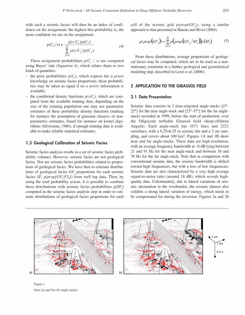
Seismic data consists in 2 time-migrated angle-stacks ([3°-22°] for the near angle-stack and [23°-37°] for the far angle-stack) recorded in 1999, before the start of production, overthe Oligocene turbidite Girassol field (deep-offshoreAngola). Each angle-stack has 1071 lines and 2221crosslines, with a 6.25×6.25 m seismic bin and a 2 ms sam-pling, and covers about 100 km2. Figures 1A and 1B shownear and far angle-stacks. These data are high-resolution,with an average frequency bandwidth at –6 dB lying between21 and 91 Hz for the near angle-stack and between 16 and76 Hz for the far angle-stack. Note that in comparison withconventional seismic data, the seismic bandwidth is shiftedtoward high frequencies, but with a loss of low frequencies.Seismic data are also characterized by a very high averagesignal-to-noise ratio (around 18 dB), which reveals high-quality data. Unfortunately, due to lateral variations of seis-mic attenuation in the overburden, the seismic dataset alsoexhibits a strong lateral variation of energy, which needs tobe compensated for during the inversion. Figures 2a and 2b

253

1 km

1 km

0.5 s

a) b)

Figure 1

Near (a) and Far (b) angle-stacks.


0

1000RMS amplitude

2.5 km

2.5 km

N

a) 0

1000RMS amplitude

2.5 km

2.5 km

N

b)

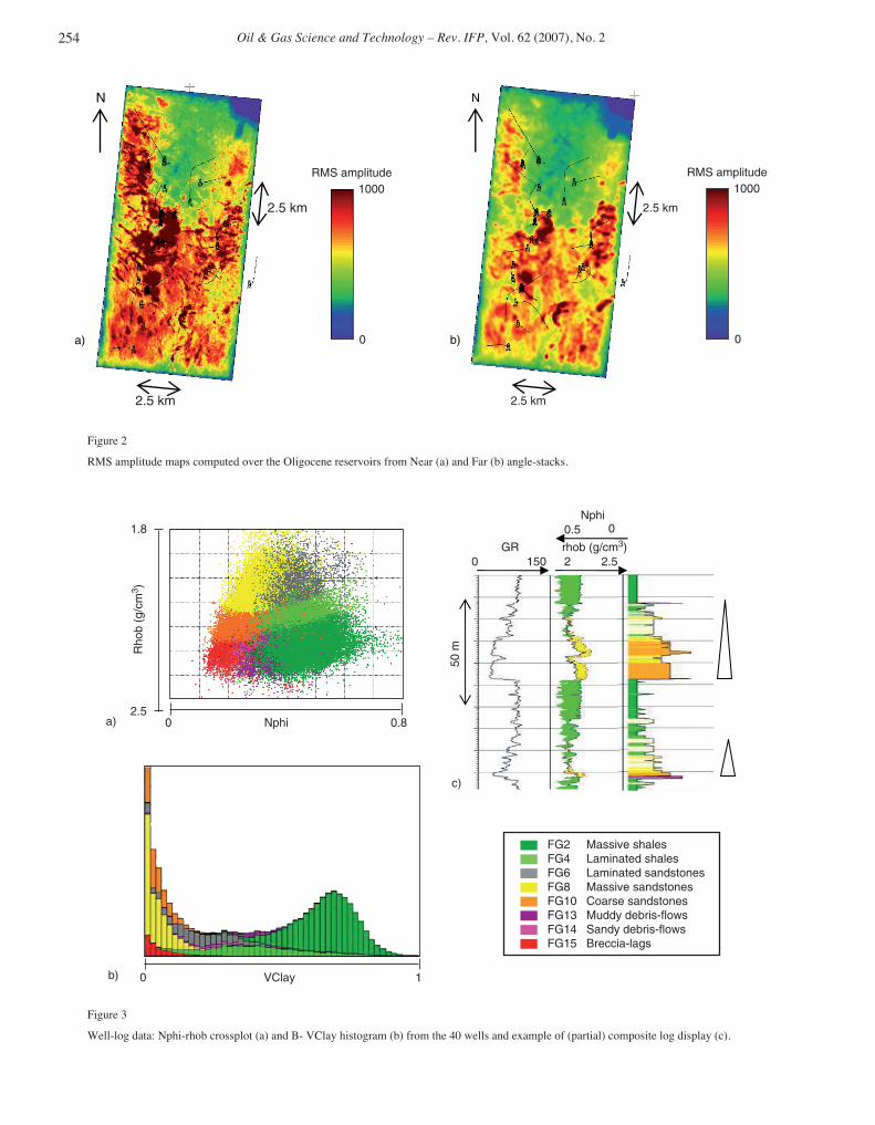
Figure 2

RMS amplitude maps computed over the Oligocene reservoirs from Near (a) and Far (b) angle-stacks.

0.8 0 Nphi

Rho

b (g

/cm

3 )

1.8

2.5

GR0 150

rhob (g/cm3)2 2.5

0.5 0Nphi

10 VClay

a)

b)

c)

50 m

FG2 Massive shalesFG4 Laminated shalesFG6 Laminated sandstonesFG8 Massive sandstonesFG10 Coarse sandstonesFG13 Muddy debris-flowsFG14 Sandy debris-flowsFG15 Breccia-lags

Figure 3

Well-log data: Nphi-rhob crossplot (a) and B- VClay histogram (b) from the 40 wells and example of (partial) composite log display (c).


display, respectively for the near and for the far angle-stacks,the variations of RMS amplitudes in the Oligocene reservoirzone. Low values in the northern part are associated withhigh attenuation.

During the study, we also consider 8 regional horizons,which delineate the main channel sequences, and a low-fre-quency velocity model (Turpin et al., 2003), derived from themigration velocity field.

Finally, we make use of the well-log database, which iscomposed of 40 wells, 13 of which provide anisotropy cor-

rected Ip and Is, as well as density (see Fig. 2a and 2b for abase-map view of the field with the well trajectories). Prior tothe beginning of the study, these well-logs have been inter-preted in terms of 8 electrofacies (Fig. 3). The first five elec-trofacies (FG2 to FG10) correspond to sediments rangingfrom massive shales (FG2), to very unconsolidated cleansandstone deposits (FG10 or “coarse sandstones”), character-ized by decreasing VClay content, as shown by Figure 3a. 3additional electrofacies have been defined to identify het-erolithic sediments (debris-flows for FG13 and FG14 and

255

Figure 4

Example of optimal time-shift mini-maps, obtained for optimal well-to-seismic calibration, in the vicinity of one well, and computed fromNear (a) and Far (b) angle-stacks.

50 m

50 m

50 m

50 m

Δt (ms)

a) b)

+32

-32

50 m

50 m

50 m

50 m

R2Chosen optimal

location

a) b)

1.0

0.5

Figure 5

Example of optimal R2 maps, obtained by comparing synthetic seismic trace from well log data and observed seismic traces, in the vicinityof one well, and computed for Near (a) and Far (b) angle-stacks.


breccia lags for FG15). The Nphi-Rhob cross-plot dis-played on Figure 3b shows that the 8 electrofacies are alsovery well discriminated in terms of porosity and density.Finally, a composite view of a particular well with its elec-trofacies interpretation (Fig. 3c) displays a clear fining-upward motif at reservoir levels, which is consistent withthe gamma-ray trend, and with channel infill successions inturbidite reservoirs.

2.2 Pre-Stack Stratigraphic Inversion

2.2.1 Well-to-Seismic Calibration

After running the Multi-Coherence analysis separately on thenear and on the far angle-stacks, a multi-well wavelet extrac-tion process is initiated with a 0-phase angle-dependentwavelet. This analysis has been performed by considering 4wells, and by extracting a 31×31 (187.5×187.5 m) corridortrace around each well path. The resulting optimal linearphase wavelets are characterized by a 0 ms average time shiftand a 10° average phase shift both on the near and on the farangle-stacks. Figures 4a and 4b display for one particularwell a map of optimal time-shifts to be applied to well-logsfor optimal match between seismic and synthetic data com-puted with the optimal linear phase wavelets. These maps arevery similar for both angle-stacks, indicating that NMOresiduals are very low. Figures 5a and 5b are the correspond-ing R2 coefficient maps between seismic and synthetic data.

Optimal well-to-seismic location is then searched in thezones with high R2 values on both angle-stacks. BecauseFigures 5a and 5b are very similar, it is very easy to find anoptimal common position to both angle-stacks (black crosson the previous maps). Finally, considering these optimallocations, the linear phase wavelets are optimized using thevariable phase and amplitude analysis. The resultingwavelets and their associated amplitude spectra are displayedrespectively on Figures 6a and 6b. As could be expected, thefrequency bandwidth is shifted to low-frequencies whenangle increases, because of NMO stretch. The computed R2

coefficients between synthetic and seismic data are veryhigh, around 0.85 for all wells, indicating good local consis-tency between seismic and well log data. Figure 7 illustrates

256

500- 50

(ms)a)

NearFar

500- 50

(ms)b)

NearFar

Figure 6

Optimal wavelets from well-to-seismic calibration (a) and corresponding amplitude spectra (b).

Synthetic

100

ms

Seismictrace

a) b)

Figure 7

Comparison between seismic trace at optimal well locationand synthetics computed from well log data and waveletsdisplayed in Figure 6; a) Near angle-stack and b) Far angle-stack.


this good fit, by comparing the seismic data extracted at anoptimal well position with the synthetic data computed fromwell log data. Additional 5 wells have then been relocated tooptimal positions using the previously estimated optimalwavelets. R2 coefficients between synthetic and seismic dataremain high for these 5 wells (> 0.7), indicating a good sta-bility of wavelet phase and origin in the Girassol field.

2.2.2 Corrections for Lateral Variations in Wavelet Energy

Well-to-seismic calibration shows that the energy ratiobetween synthetic and seismic data varies between wells. Ifwe had not compensated for these variations, the inversionprocedure would tend to under-estimate the reflection coeffi-cients in attenuated zones. The resulting Ip and Is valueswould therefore be erroneous. To compensate for theseenergy variations, we have to compute for each angle-stack awavelet multiplier map, the role of which is to incorporatethe attenuation effects on the wavelets, thereby allowing avalid estimation of reflection coefficients. Moreover, thesemaps should be constrained at well positions to be consistentwith the local synthetic-to-seismic energy ratio computedduring well-to-seismic calibration. Therefore, we have inter-polated the wavelet multipliers computed at wells by kriging,taking smoothed RMS amplitude maps (Fig. 2a and 2b) asexternal drifts. Figures 8a and 8b display the resultingwavelet multiplier maps for respectively the near and the farangle-stack.

2.2.3 A priori Model Construction

The procedure interpolates well logs along correlation sur-faces, which have to reflect the stratigraphic framework ineach geological unit. Seismic modeling tools (Bourgeois etal., 2004) have been used extensively at this stage to deter-mine the most realistic stratigraphic setting for each unit.Figure 9 illustrates one of these tests, where a conceptualgeological model has been considered under different strati-graphic hypotheses. After comparing the modeled seismicwith observed seismic, the preferred model was finally paral-lel to top for the displayed channel sequence.

To better constrain the low-frequency component of thismodel, which cannot be updated by inversion, we have inte-grated a velocity model (Turpin et al., 2003) in the interpola-tion procedure. The quality of this velocity model, which givesinformation in the 0-3 Hz frequency range, has first been testedby comparison with low-frequency velocity well log data.Since the correlation between these data is reasonnably good(R2 = 0.75), the velocity model could be used to constrain theinterpolation of well log data. Figures 10A and 10B display thesmoothly varying Ip and Is a priori model.

2.2.4 Joint Pre-Stack Inversion

Figures 11A and 11B Ip and Is obtained by stratigraphicinversion. Both results exhibit very good spatial resolution,which is better than that of the seismic amplitudes: a high-impedance sinuous shale plug is clearly visible both on Ip and

257

0.6

1.8

2.5 km

2.5 km

N

a) 0.6

1.8

2.5 km

2.5 km

N

b)

Figure 8

Wavelet multiplier maps obtained to compensate for seismic attenuation lateral variations for Near (a) and Far (b) angle-stack.


Is results. Low-impedance anomalies located inside themeanders correspond to reservoir sandstones. Note also thatthese anomalies tend to be less visible towards the South,which is due to the influence of structure: southern area arelocated on the edges of the anticline, and therefore will tendto have higher impedances. Thanks to the whitening of thespectra obtained through inversion, the vertical resolution ofthese results is also improved: at –6 dB, the Ip reflection coef-ficient bandwidth reaches 130 Hz, while the Is reflection

coefficient bandwidth reaches 110 Hz. These values can becompared with the 91 Hz and 76 Hz upper limits of respec-tively the near and far angle-stacks.

To validate the inversion results, we first examine theresidual amplitude volumes, which are the differencebetween initial amplitudes and synthetics associated withthe optimal model (Fig. 12a and 12b, where the palettedynamics is the same as on Figures 1a and 1b). On bothangle-stacks, residuals have low energy, and exhibit no

258

sandstones

massive shales

laminated

shales

1 km

50 m

a)

b) c)

4000

5500

1900

2900

1 km 1 km

0.5 s

Ip(g/cm3m/s)

Is(g/cm3m/s)

a) b)

Figure 9

Conceptual geological model with a layering parallel to top in channel area (a) associated with seismic data (c), and synthetic seismic (b)computed from the geological model (a).

Figure 10

A priori models for Ip (a) and Is (b).


coherent spatial character; they contain mainly noise. Asecond quality check is made at well locations. Weobserve a good agreement between inversion results andwell logs (Fig. 13a). More globally, when comparinginversion results with low-pass filtered well-logs (Fig.13b for Ip and 13c for Is), we observe the inversionresults are globally unbiased (no systematic departurefrom the red line, which corresponds to the first bissectorline). Finally, dispersion in these cross-plots around thisbisector line remains reasonable: the R2 coefficient com-puted between these data and the first bissector line isrespectively 0.75 for Ip and 0.70 for Is. The inversionresults can therefore be considered as good quality(although not perfectly matching well data). They cannow be interpreted in terms of seismic facies.

2.3 Seismic Facies Analysis

Prior to run 3D seismic facies analysis, the first issues to beaddressed concern the definition of seismic facies andseismic attributes used to discriminate between the differentseismic facies.

The simplest solution to integrate the geological informa-tion contained in the electrofacies interpretation of well-logdata (Fig. 3c) could be to use directly well data as the train-ing database to calibrate the classification function and thenapply this calibrated relationship to predict facies elsewherein the interwell space. However, one has to be very carefulwhile applying this type of approach since:– well data (logs and geological facies) and seismic data are

not defined at the same scale and resolution;

259

4000

5500

1900

2900

1 km 1 km

0.5 s

Ip(g/cm3m/s)

Is(g/cm3m/s)

a) b)

Figure 11

Optimal models for Ip (a) and Is (b).

1 km

1 km

0.5 s

a) b)

Figure 12

Residual amplitudes after stratigraphic inversion for Near (a) and Far (b) angle-stacks.


– seismic information is generally poorer than well informa-tion: typically, we will only dispose of 2 independent quan-tities derived from inverted Ip and Is to discriminatebetween seismic facies, in comparison with the whole suiteof well-logs available to discriminate geological facies.To address these issues and try to keep a geological con-

straint in seismic facies definition, we have successivelytested the discrimination between the geological facies atwell-log scale and then at seismic scale.

2.3.1 Discrimination at Well-Log Scale

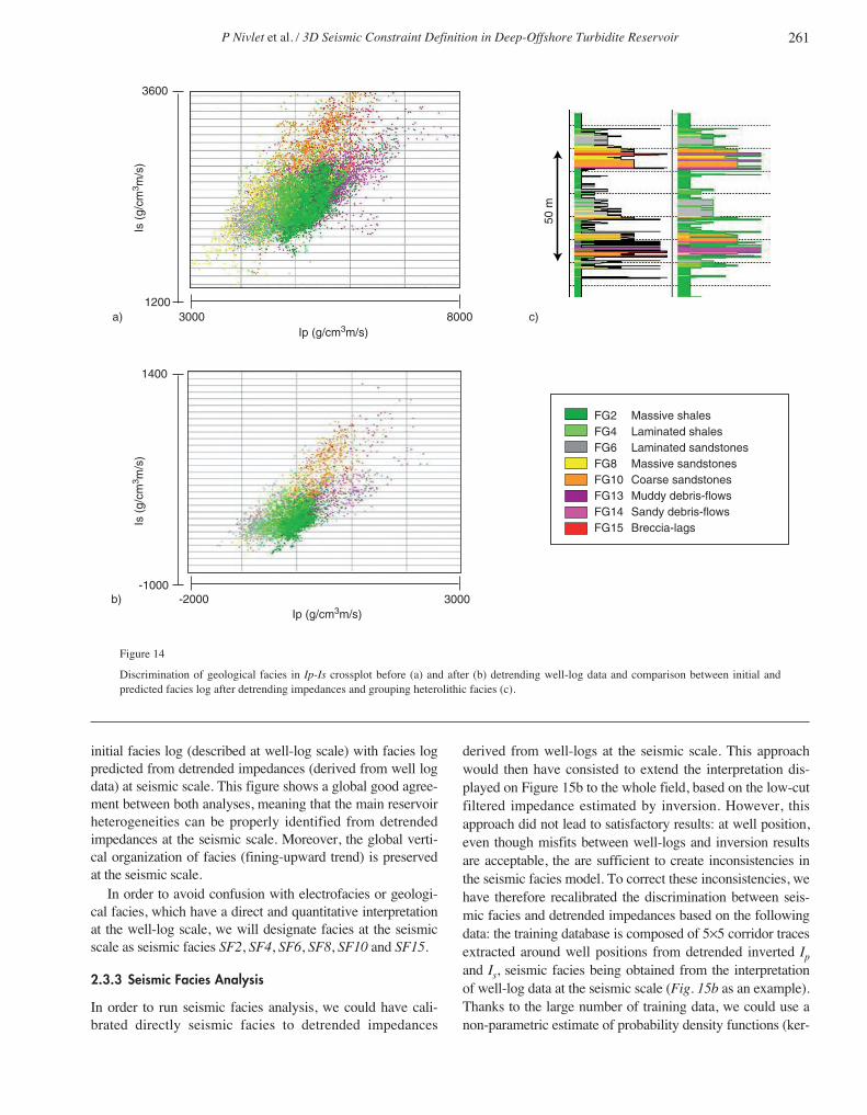
Figure 14a, which displays well data, interpreted in terms ofgeological facies projected in Ip-Is crossplot, clearly shows thatdiscrimination is not possible using only Ip and Is: the globalrate of agreement obtained by direct reassignment test on thetraining database is as low as 50%, meaning that it is only pos-sible to correctly interpret half of the well from Ip and Is.

One of the causes for this low agreement rate is the com-paction effect, which results in a global increase of imped-ances with depth. In the Girassol field, this effect is remark-able due to the anticline structure of the field and to thecomplex history of deposition, which results in multiplereservoir intervals. To attenuate this effect, Ip and Is havebeen detrended by filtering out the low-frequency component

(0-0-4-8 Hz) of Ip and Is. Figure 14b displays that the dis-crimination between the facies has been greatly improved.Quantitatively, the direct reassignment test score increases to63%, which is essentially due to a better identification offacies FG2, FG6 and FG10. However, the three “heterolithicfacies” (FG13, FG14 and FG15) remain poorly discrimi-nated one from the other. Consequently, these three facieshave been grouped into a single facies group. The direct reas-signment test score after this operation is 68%, which isacceptable for going on with the analysis. Figure 14c showsat a particular well that facies analysis results from detrendedimpedances and initial electrofacies at a particular well, areglobally in good agreement.

As a summary, discrimination between geological faciesfrom impedances is possible after removing the low-fre-quency trend from impedances, and after grouping het-erolithic facies. In the following, we will consider thesedetrended attributes and 6 facies.

2.3.2 Discrimination at Seismic Scale

Since seismic data are defined at a coarser scale than well-logdata, discrimination between the 6 facies mentionned abovefrom detrended impedances should be also tested at seismicscale, prior to apply it to inverted data. Figure 15 compares

260

Well log

Inversionresult

100

ms

Ip Is3500 7500 1000 4000

a)

3500

7500(g/cm3.m/s)

75003500b)

1000 40001000

4000

c)Figure 13

Comparison between low-pass filtered impedances from well-log data and inversion results for one well (a), and cross-plot betweeninversion results and low-pass filtered well-logs for Ip (b) and Is (c).


initial facies log (described at well-log scale) with facies logpredicted from detrended impedances (derived from well logdata) at seismic scale. This figure shows a global good agree-ment between both analyses, meaning that the main reservoirheterogeneities can be properly identified from detrendedimpedances at the seismic scale. Moreover, the global verti-cal organization of facies (fining-upward trend) is preservedat the seismic scale.

In order to avoid confusion with electrofacies or geologi-cal facies, which have a direct and quantitative interpretationat the well-log scale, we will designate facies at the seismicscale as seismic facies SF2, SF4, SF6, SF8, SF10 and SF15.

2.3.3 Seismic Facies Analysis

In order to run seismic facies analysis, we could have cali-brated directly seismic facies to detrended impedances

derived from well-logs at the seismic scale. This approachwould then have consisted to extend the interpretation dis-played on Figure 15b to the whole field, based on the low-cutfiltered impedance estimated by inversion. However, thisapproach did not lead to satisfactory results: at well position,even though misfits between well-logs and inversion resultsare acceptable, the are sufficient to create inconsistencies inthe seismic facies model. To correct these inconsistencies, wehave therefore recalibrated the discrimination between seis-mic facies and detrended impedances based on the followingdata: the training database is composed of 5×5 corridor tracesextracted around well positions from detrended inverted Ipand Is, seismic facies being obtained from the interpretationof well-log data at the seismic scale (Fig. 15b as an example).Thanks to the large number of training data, we could use anon-parametric estimate of probability density functions (ker-

261

80003000

3600

1200

3000-2000

1400

-1000

50 m


a) c)

b)

Ip (g/cm3m/s)

Ip (g/cm3m/s)

Is (

g/cm

3 m/s

) Is

(g/

cm3 m

/s)

Figure 14

Discrimination of geological facies in Ip-Is crossplot before (a) and after (b) detrending well-log data and comparison between initial andpredicted facies log after detrending impedances and grouping heterolithic facies (c).


nel method). The cross-validation tests performed on thetraining database gave excellent results with an average of85% of training data correctly discriminated. The classifica-tion function has then been used to predict 6 seismic faciesprobability cubes. Figures 16a and 16b display the mostprobable seismic facies cube, and its associated probabilitycube. It displays the spatial organization of seismic facies fora typical channel sequence; a fining-upward trend of seismicfacies (from orange to grey) can be seen. Laterally, channelsare surrounded by green seismic facies, which are interpretedas silty levees. Probabilities associated to this interpretationare high; they are slightly lower in the channel sequences,where geology changes rapidly. In conclusion, 3D seismicfacies analysis identifies qualitatively the main geological fea-tures of Girassol field. However, this interpretation is incom-plete for two main reasons: first, seismic facies are notdirectly linked with geological facies since seismic resolution

is limited with respect to the size of geological hetero-geneities; and second, probabilities cannot be interpreted asproportions of geological facies. Consequently, seismic faciesanalysis results need to be recalibrated to geology.

2.4 Construction of 3D Seismic Constraint

Use of equation 5 allows computation of the expected pro-portions of geological facies by combining seismic faciesproportions with distributions of geological facies propor-tions from seismic facies estimated at well positions.However, such direct derivation may not be very useful forseismic constraint definition, since distributions of geologicalfacies proportions display a lot of dispersion (see Fig. 17 fordistributions of geological facies proportions for seismicfacies SF8). This dispersion is due to the non-uniqueness of

262

50 m

Grouped at theseismic scale


a) b)

Figure 15

Comparison between initial electrofacies interpretation of well log data (a), compared with interpretation of detrended Ip and Is at the seismicscale (b).

0

1

1 km 1 km

0.5 s

Is(g/cm3m/s)

a) b)

SF2

SF4

SF6

SF8

SF10

SF15

Figure 16

Most probable seismic facies (a) and associated probability (b).


the correspondence between geological facies proportionsand seismic facies, which varies spatially.

In order to better constrain the computation of geologicalfacies proportion by seismic facies required by Equation 5,we have considered separately the computation of geologicalfacies proportions in each of the 9 “geological units” alreadyused to build the a priori model for inversion. We have there-fore taken into account “stratigraphic” non-stationnarity inthe computations. Figures 18a and 18b show resulting aver-age shale and sandstone proportion volumes. Reservoirs arevery well delineated in these displays.

As an ultimate quality control of this analysis, verticalproportion curves extracted at well positions fit very wellwith vertical proportion curves obtained from the upscalingof electrofacies at the seismic scale (Fig. 19).

CONCLUSIONS

This paper has described a workflow to characterize Girassolreservoir properties from seismic data acquired before thestart of production. This work has benefited from the excel-lent spatial resolution of the seismic data. We have shownthat building a 3D constraint from seismic for geologicalmodeling was not straightforward. It has first required a pre-stack inversion, which allows estimating an optimal elasticparameter model from seismic amplitudes, while increasingthe resolution of seismic. This first phase has clearly shownthe importance of properly calibrating seismic with other datasuch as well logs. It has also shown that because of the sizeof the seismic cubes, the hypothesis that the wavelet was sta-tionary over the whole seismic cube was wrong, and that itwas necessary to correct for this assumption. From the resultsof the inversion, we could derive seismic facies probabilitycubes. In order to obtain meaningful results we have first per-formed a detailed analysis of well data to build the faciesdatabase, then applied an appropriate impedance detrendingto compensate for compaction and finally analysed the verti-cal upscaling process from the log to the seismic scale andexecuted a non-linear interpretation of seismic attribute cubesbefore recalibrating the resulting seismic facies to geology.

Despite the high resolution of the resulting seismic con-straint, some improvements may be achieved, especially bybetter estimating the non-stationnarity in the last seismic con-straint definition phase.

These cubes have been used in further work as a non-sta-tionary constraint to build an initial detailed geostatisticalgeological model (Lerat et al., 2006), which will be used asan input in history matching, constrained with 4D seismicdata (Mezghani et al., 2004).

ACKNOWLEDGEMENTS

The authors would like to thank SONANGOL, SociedadeNacional de Combustíveis de Angola, Esso Exploration

263

0

100

0

100

1 km 1 km

0.5 s

a) b)

Figure 18

Average sandstone (a) and shale (b) proportions (in %).

B

Pro

port

ion

(%)

0

100

Mas

sive

shale

s

Lam

inate

d sh

ales

Lam

inate

d sa

ndsto

nes

Mas

sive

sand

stone

s

Coars

e sa

ndsto

nes

Mud

dy d

ebris

-flow

s

Sandy

deb

ris-fl

ows

Brecc

ia-lag

s

Figure 17

Distributions (box-plots) of geological facies proportions forseismic facies SF8 obtained on the whole well database.


Angola (Block 17), BP Exploration (Angola), Statoil AngolaBlock 17 A.S., Norsk Hydro, Total Angola and Total for per-mission to present this paper. Olivier Lerat, Thierry Tonellot,Nathalie Lucet and Frédéric Roggero are also acknowledgedfor the fruitful discussions and contributions to some aspectsof this paper.

REFERENCES

Aki, K. and Richards, P.G. (2002) Quantitative seismology: Theoryand methods, 2nd edition. University Science Books, Sausalito.Barens, L. and Biver, P. (2004) Reservoir facies prediction fromgeostatistical inverted data. SPE - 11th International PetroleumConference and Exhibition, paper 88690.Bourgeois, A. Joseph, P. and Lecomte, J.-C. (2004) Three-dimen-sional full wave seismic modelling versus one-dimensional convo-lution: the seismic appearance of the Grès d’Annot turbidite system.Geol. Soc. London, 221, S401-S417.Dash, B.L. and Obaidullah, K.A. (1970) Determination of signal andnoise statistics using correlation theory. Geophysics, 35, 24-32.Doligez, B., Gomel, P., Andrieux, B., Fournier, F. and Beucher, H.(2003) Use of seismic to constrain geostatistical reservoir models: aquantitative approach using proportions of facies. AAPG - AnnualConvention, Salt Lake City, 11-14 May, paper 78165.Fournier, F., and Derain, J.-F. (1995) A statistical methodology forderiving reservoir properties from seismic data. Geophysics, 60,1437-1450.

Hand, D.J. (1981) Discrimination and classification. Wiley Seriesin Probabilities and Mathematical Statistics, John Wiley & Sons,Chichester.Hohn, M.E. , McDowell, R.R., Matchen, D.L., and Vargo, A.G.(1997) Heterogeneity of Fluvial-Deltaic Reservoirs in theAppalachian Basin: A Case Study from a Lower Mississippian OilField in Central West Virginia. AAPG Bull., 81, 918-936.Lefeuvre, F., Kerdraon, Y., Peliganga, J., Medina, S., Charrier, P.,L’Houtellier, R. and Dubucq, D. (2003) Improved reservoir under-standing through rapid and effective 4D: Girassol field, Angola,West Africa. SEG - 73rd Annual International Meeting, Dallas, 26-31 October. Expanded Abstracts, 1338-1341.Lerat, O., Doligez, B., Albouy, E., Nivlet, P., Roggero, F., Cap, J.,Vittori, J. and Duplantier, O. (2006) Integrated reservoir model:geostatistical geological modeling using a 3D seismic constraint.GCSSEPM - 26th Annual Bob F. Perkins Research Conference,Reservoir Characterization: Integrating technology and businesspractices, 3-6 December, Houston, Texas.Lucet, N., Déquirez, P.-Y. and Cailly, F. (2000) Well-to-seismiccalibration: A multiwell analysis to extract one single wavelet. SEG- 70th Annual International Meeting, Calgary, 6-11 August.Expanded abstracts, 1615-1618.Mezghani, M., Fornel, A., Langlais, V., and Lucet, N. (2004)History matching and quantitative use of 4D seismic data for animproved reservoir characterization. SPE Annual TechnicalConference and Exhibition, Houston, 26-29 September. SPE 90420.Navarre, J.-C., Claude D., Liberelle, E., Safa, P., Vallon, G., andKeskes, N. (2002) Deepwater turbidite system analysis, WestAfrica: Sedimentary model and implications for reservoir modelconstruction. The Leading Edge, 21, 1132-1139.Nivlet, P. (2004) Low-frequency constraint in a priori model build-ing for stratigraphic inversion. SEG- 74th Annual InternationalMeeting, Denver, 10-15 October. Expanded abstracts, 1802-1805.Nivlet, P., Doligez, B., Dos Santos, M.-S., Dillon L., andSchwedersky-Neto, G. (2004) Seismic facies interpretation in a tur-biditic environment from pre-stack data: a case study. 66th EAGEConference & Exhibition, Paris, 6-10 June. D04, ExtendedAbstracts.Silverman, B.W. (1986) Density estimation for statistical and dataanalysis. Chapman and Hall, London.Tarantola, A. (1987) Inverse problem theory. Elsevier, New-York.Tonellot, T., Macé, D. and Richard, V. (2001) Joint stratigraphicinversion of angle-limited stacks. SEG - 71st Annual InternationalMeeting, San Antonio, 9-14 September. Expanded abstracts, 227-230.Turpin P., Gonzalez-Carballo A., Bertini F., and Lefeuvre, F. (2003)Velocity volume and time/depth conversion approach duringGirassol field development. SEG - 73rd Annual InternationalMeeting, Dallas, 26-31 October. Expanded abstracts, 2179-2182.

Final manuscript received in July 2006

264

50 m

s

50 m

s

a) b)

Figure 19

Comparison for two wells between electrofaciesinterpretation of well logs, Vertical proportion curve derivedthere from at the seismic scale and proportions computedfrom seismic data.

Copyright © 2007 Institut français du pétrolePermission to make digital or hard copies of part or all of this work for personal or classroom use is granted without fee provided that copies are not madeor distributed for profit or commercial advantage and that copies bear this notice and the full citation on the first page. Copyrights for components of thiswork owned by others than IFP must be honored. Abstracting with credit is permitted. To copy otherwise, to republish, to post on servers, or to redistributeto lists, requires prior specific permission and/or a fee: Request permission from Documentation, Institut français du pétrole, fax. +33 1 47 52 70 78, or [email protected].

3D Seismic Constraint Definition in Deep-Offshore Turbidite Reservoir

Documents

Transcript of 3D Seismic Constraint Definition in Deep-Offshore Turbidite Reservoir