3D OBJECT 3D OBJECT REPRESENTATIONSREPRESENTATIONS

CEng 477Introduction to Computer Graphics

Fall 2007­2008

Object Representations

● Types of objects:geometrical shapes, trees, terrains, clouds, rocks, glass, hair, furniture, human body, etc.

● Not possible to have a single representation for all– Polygon surfaces– Spline surfaces– Procedural methods– Physical models– Solid object models– Fractals– ……

Two categories

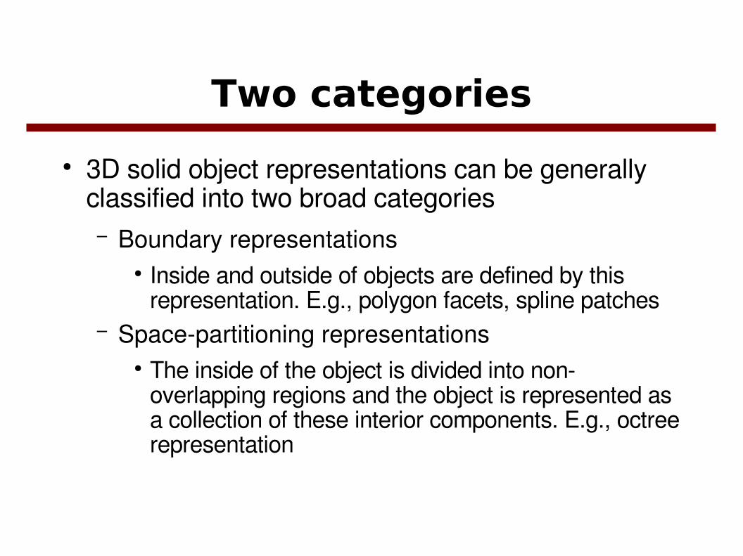
● 3D solid object representations can be generally classified into two broad categories– Boundary representations

● Inside and outside of objects are defined by this representation. E.g., polygon facets, spline patches

– Space­partitioning representations● The inside of the object is divided into non­

overlapping regions and the object is represented as a collection of these interior components. E.g., octree representation

Polygon Surfaces (Polyhedra)

● Set of adjacent polygons representing the object exteriors.● All operations linear, so fast.● Non­polyhedron shapes can be approximated by polygon 

meshes.● Smoothness is provided either by increasing the number of 

polygons or interpolated shading methods.

Levels of detail Interpolated shading

Data Structures

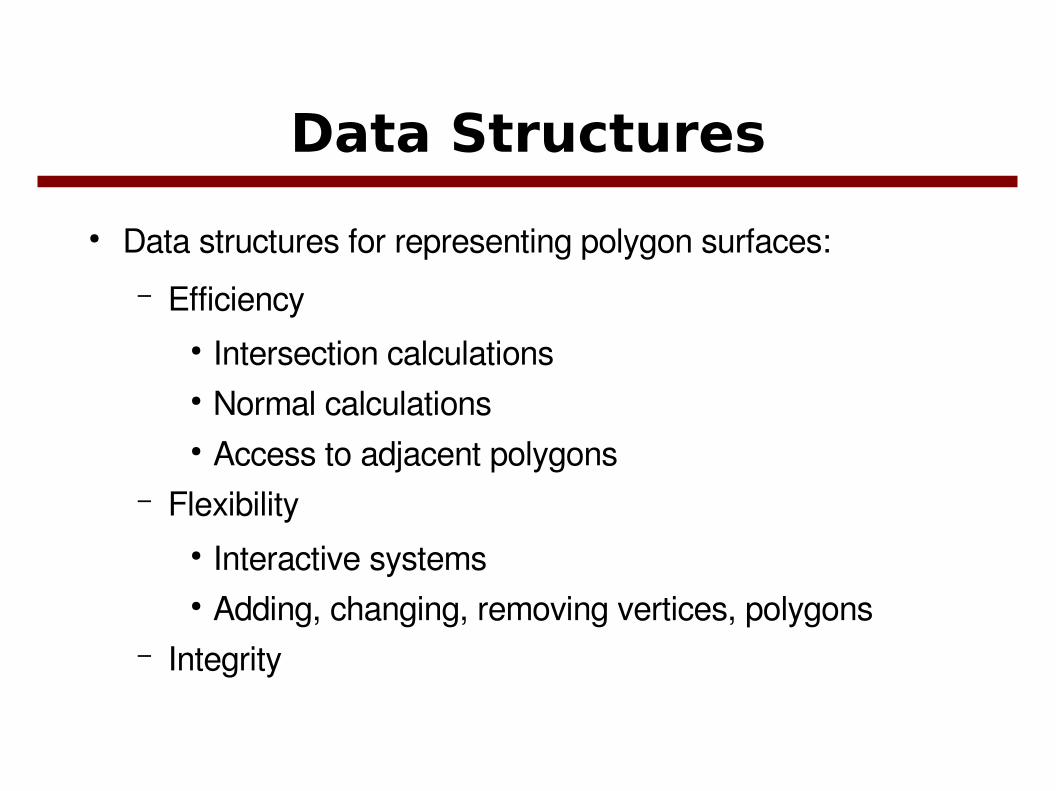
● Data structures for representing polygon surfaces:– Efficiency

● Intersection calculations● Normal calculations● Access to adjacent polygons

– Flexibility● Interactive systems● Adding, changing, removing vertices, polygons

– Integrity

Polygon Tables

● Vertices   Edges   Polygons

● Forward pointers:i.e. to access adjacent surfacesedges

V1

V2

V3

V4

V7

V8

V6

V5

E1

E2

E3

E4

E6E11

E7

E10E9

E8

E5V1:(x1,y1,z1)V2:(x2,y2,z2)V3:(x3,y3,z3)V4:(x4,y4,z4)V5:(x5,y5,z5)V6:(x6,y6,z6)V7:(x7,y7,z7)V8:(x8,y8,z8)

E1: V1,V2

E2: V2,V3

E3: V2,V5

E4: V4,V5

E5: V3,V4

E6: V4,V7

E7: V7,V8

E8: V6,V8

E9: V1,V6

E10: V5,V6

E11: V5,V7

S1: E1,E3,E10,E9

S2: E2,E5,E4,E3

S3: E10,E11,E7,E8

S4: E4,E6,E11

V1: E1,E9   

V2: E1,E2,E3

V3: E2,E5   V4: E4,E5,E6

V5: E3,E4E10,E11  

V6: E8,E9,E10

V7: E6,E7,E11   

V8: E7,E8

E1: S1   

E2: S2

E3: S1,S2  

E4: S2,S4

E5: S2   E6: S4

E7: S3   E8: S3

E9: S1   E10: S1,S3

E11: S3,S4

● Additional geometric properties:– Slope of edges– Normals– Extends (bounding box)

● Integrity checks 

∀V , ∃Ea , Eb such that V∈Ea ,V∈Eb

∀ E , ∃S such that E∈S

∀ S , S  is closed

∀ S1, ∃S2  such that  S1∩S2≠∅

Sk  is listed in  Em⇔E m  is listed in  Sk

Polygon Meshes

● Triangle strips:123, 234, 345, ..., 10 11 12

1 2 3 4 5 6 7 8 9 10 11 12

● Quadrilateral meshes:n×m array of vertices

1 3

2 4

5

6

7

8

9

10

11

12

Plane Equations

● Equation of a polygon surface:

● Surface Normal:

A xB yC zD=0Linear set of equations:A /Dx kB /D ykC /D z k=−1, k=1, 2,3

A=y1z2−z3y2 z3−z1y3z1−z2

B=z1x2−x3z2 x3−x1z3x1−x2

C=x1y2−y3x2y3−y1x3y1−y2

D=−x1y2 z3−y3 z2−x2y3 z1−y1 z3−x3y1 z2−y2 z1

N=A , B ,C

extracting normal from vertices:N=V 2−V 1×V 3−V 1

V1

V2

V3

Counterclockwiseorder.

● Find plane equation from normal and a point on the surface

● Inside outside tests of the surface (N is pointing towards outside):

A , B ,C =NN⋅x , y , zD=0P  is a point in the surface (i.e. a vertex) D=−N⋅P

A xB yC zD0 ,  point is inside the surfaceA xB yC zD0 ,  point is outside the surface

OpenGL Polyhedron Functions

● There are two methods in OpenGL for specifying polygon surfaces.– You can use geometric primitives, GL_TRIANGLES, 

GL_QUADS, etc. to describe the set of polygons making up the surface

– Or, you can use the GLUT functions to generate five regular polyhedra in wireframe or solid form.

Drawing a sphere with GL_QUAD_STRIP

void drawSphere(double r, int lats, int longs) {int i, j; for(i = 0; i <= lats; i++) {

double lat0 = M_PI * (­0.5 + (double) (i ­ 1) / lats); double z0 = sin(lat0);double zr0 = cos(lat0); double lat1 = M_PI * (­0.5 + (double) i / lats); double z1 = sin(lat1);double zr1 = cos(lat1);glBegin(GL_QUAD_STRIP); for(j = 0; j <= longs; j++) {

double lng = 2 * M_PI * (double) (j ­ 1) / longs; double x = cos(lng);double y = sin(lng); glVertex3f(x * zr0, y * zr0, z0); glVertex3f(x * zr1, y * zr1, z1); 

}glEnd();

}} 

You will not see it like this untilyou learn “lighting”.

Five regular polyhedra provided by GLUT

Also called Platonicsolids.

The faces are identical regular polygons.

All edges, edge angles are equal. 

Tetrahedron

● glutWireTetrahedron ( );● glutSolidTetrahedron ( );● This polyhedron is generated with its center at the 

world­coordinate origin and with a radius equal to 3

Cube

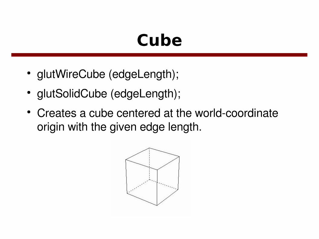
● glutWireCube (edgeLength);● glutSolidCube (edgeLength);● Creates a cube centered at the world­coordinate 

origin with the given edge length.

Octahedron

● glutWireOctahedron ( );● glutSolidOctahedron ( );● Creates a octahedron with 8 equilateral triangular 

faces. The radius is 1.

Dodecahedron

● glutWireDodecahedron ( );● glutSolidDodecahedron ( );● Creates a dodecahedron centered at the world­

coordinate origin with 12 pentagon faces.

Icosahedron

● glutWireIcosahedron ( );● glutSolidIcosahedron ( );● Creates an icosahedron with 20 equilateral 

triangles. Center at origin and the radius is 1.

Curved Surfaces

● Can be represented by either parametric or non­parametric equations. 

● Types of curved surfaces– Quadric surfaces– Superquadrics– Polynomial and Exponential Functions– Spline Surfaces

Quadric Surfaces

● Described with second degree (quadric) equations. ● Examples:

– Spheres– Ellipsoids– Tori– Paraboloids– Hyperboloids

● Can also be created using spline representations.

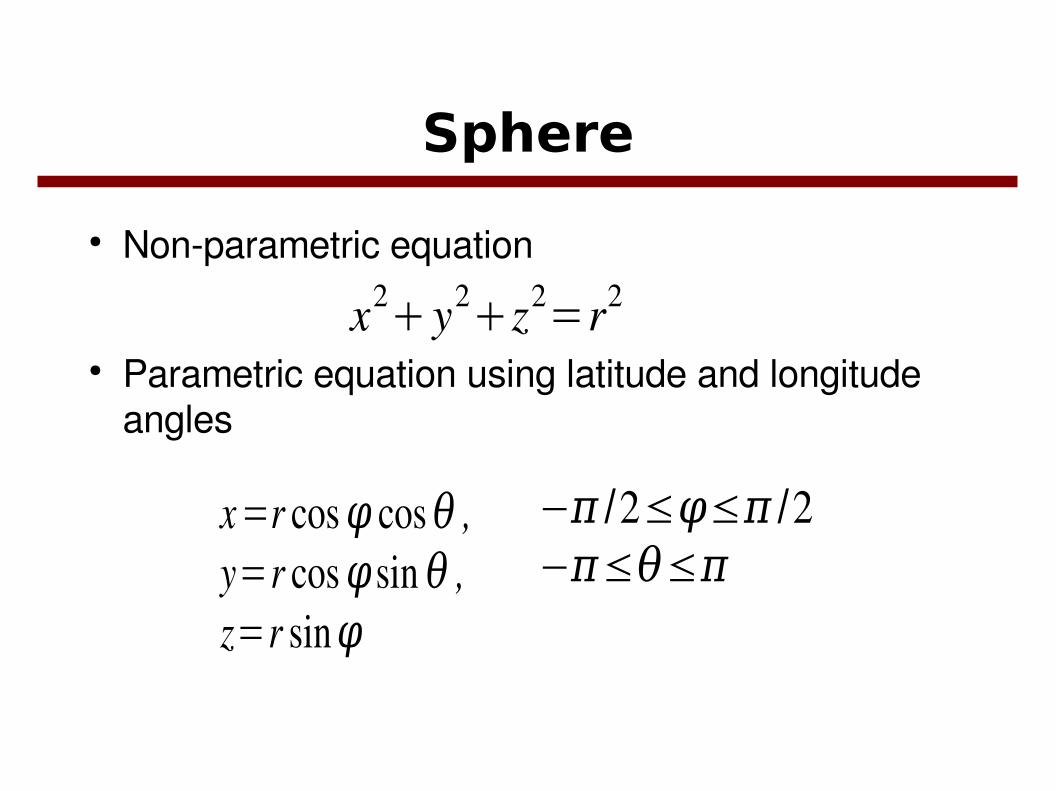
Sphere

● Non­parametric equation

● Parametric equation using latitude and longitude angles

x2 y2

z2=r2

x=r cosφ cosθ ,y=r cosφsin θ ,z=r sinφ

−π /2≤φ≤π /2−π≤θ≤π

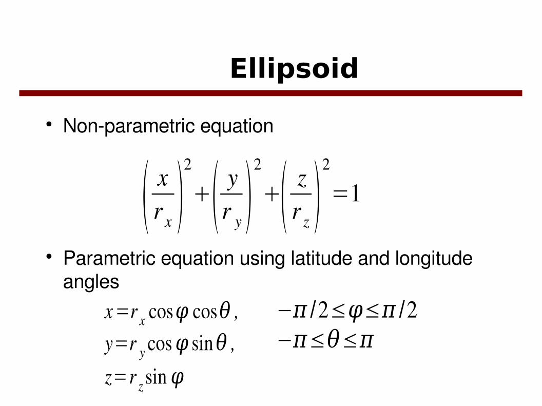
Ellipsoid

● Non­parametric equation

● Parametric equation using latitude and longitude angles

xr x

2

yr y

2

zr z

2

=1

x=r x cosφ cosθ ,y=r y cosφ sinθ ,

z=r z sinφ

−π /2≤φ≤π /2−π≤θ≤π

Superquadrics

● Adding additional parameters to quadric representations to get new object shapes.

●  One additional parameter is added to curve (i.e., 2d) equations and two parameters are added to surface (i.e., 3d) equations.

Superellipse

xr x

2/ n

yr y

2 /n

=1x=r x cosnθ ,

y=r y sinnθ

−π≤θ≤π

r x=r y

Superellipse

● Used by industrial designers often

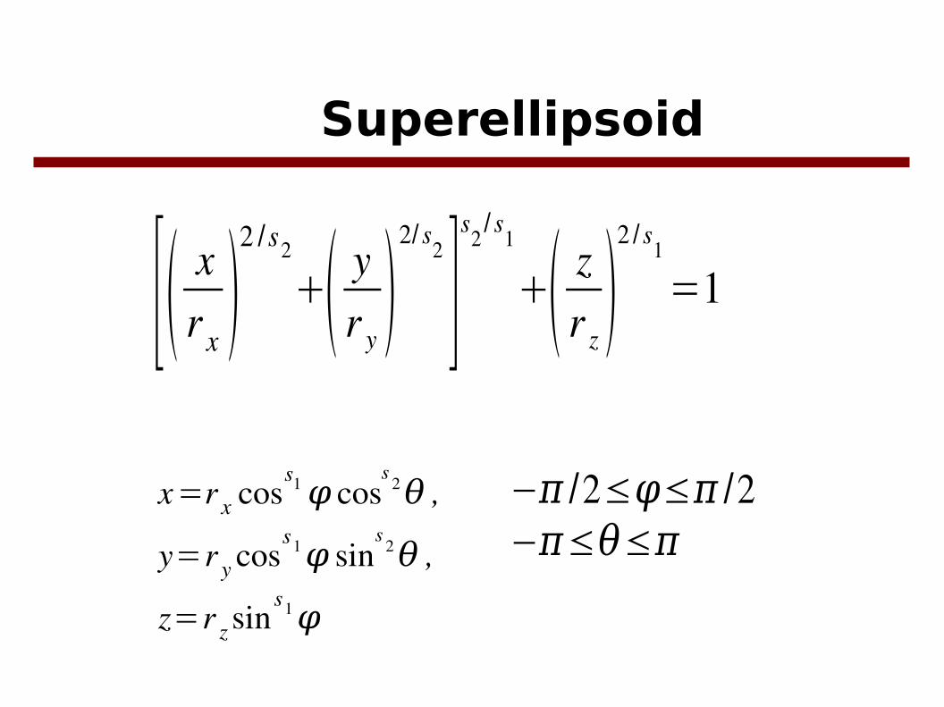
Superellipsoid

[xr x

2 /s2

yr y

2/ s2

]s

2/ s

1

zr z

2 / s1

=1

x=r x coss1 φ cos

s2θ ,

y=r y coss1φ sin

s2θ ,

z=r z sins1φ

−π /2≤φ≤π /2−π≤θ≤π

Superellipsoid

OpenGL Quadric-Surface and Cubic-Surface Functions

● GLUT and GLU provide functions to draw quadric­surface objects.

● GLUT functions– Sphere, cone, torus

● GLU functions– Sphere, cylinder, tapered cylinder, cone, flat circular 

ring (or hollow disk), and a section of a circular ring (or disk)

● GLUT also provides a function to draw a “teapot” (modeled with bicubic surface pathces). 

Examples

GLUT sphere

GLUT cone

GLU cylinder

GLUT functions

● glutWireSphere (r, nLongitudes, nLatitudes);● glutSolidSphere (r, nLongitudes, nLatitudes);● glutWireCone(rBase, height, nLong, nLat);● glutSolidCone(rBase, height, nLong, nLat);● glutWireTorus(rCrossSection, rAxial, nConcentric, nRadial);● glutWireTorus(rCrossSection, rAxial, nConcentric, nRadial);● glutWireTeapot(size);● glutSolidTeapot(size);

GLU Quadric-Surface Functions

● GLU functions are harder to use.● You have to assign a name to the quadric. ● Activate the GLU quadric renderer● Designate values for the surface parameters● Example:

GLUquadricObj *mySphere;mySphere = gluNewQuadric();gluQuadricStyle (mySphere, GLU_LINE);gluSphere (mySphere, r, nLong, nLat);

Quadric styles

● Other than GLU_LINE we have the following drawing styles:– GLU_POINT– GLU_SILHOUETTE– GLU_FILL

Other GLU quadric objects

● gluCylinder (name, rBase, rTop, height, nLong, nLat);

● gluDisk (name, rInner, rOuter, nRadii, nRings);● gluPartialDisk (… parameters …);

Additional functions to manipulate GLU quadric

objects● gluDeleteQuadric (name);● gluQuadricOrientation (name, normalDirection);

– To specify front/back directions.– normalVector is GLU_INSIDE or GLU_OUTSIDE

● gluQuadricNormals (name, generationMode);– Mode can be GLU_NONE, GLU_FLAT, or 

GLU_SMOOTH based on the lighting conditions you want to use for the quadric object.

Spline Representations

● Spline curve: Curve consisting of continous curve segments approximated or interpolated on polygon control points.

● Spline surface: a set of two spline curves matched on a smooth surface.

● Interpolated: curve passes through control points● Approximated: guided by control points but not necessarily 

passes through them.

InterpolatedApproximated

● Convex hull of a spline curve: smallest polygon including all control points.

● Characteristic polygon, control path: vertices along the control points in the same order.

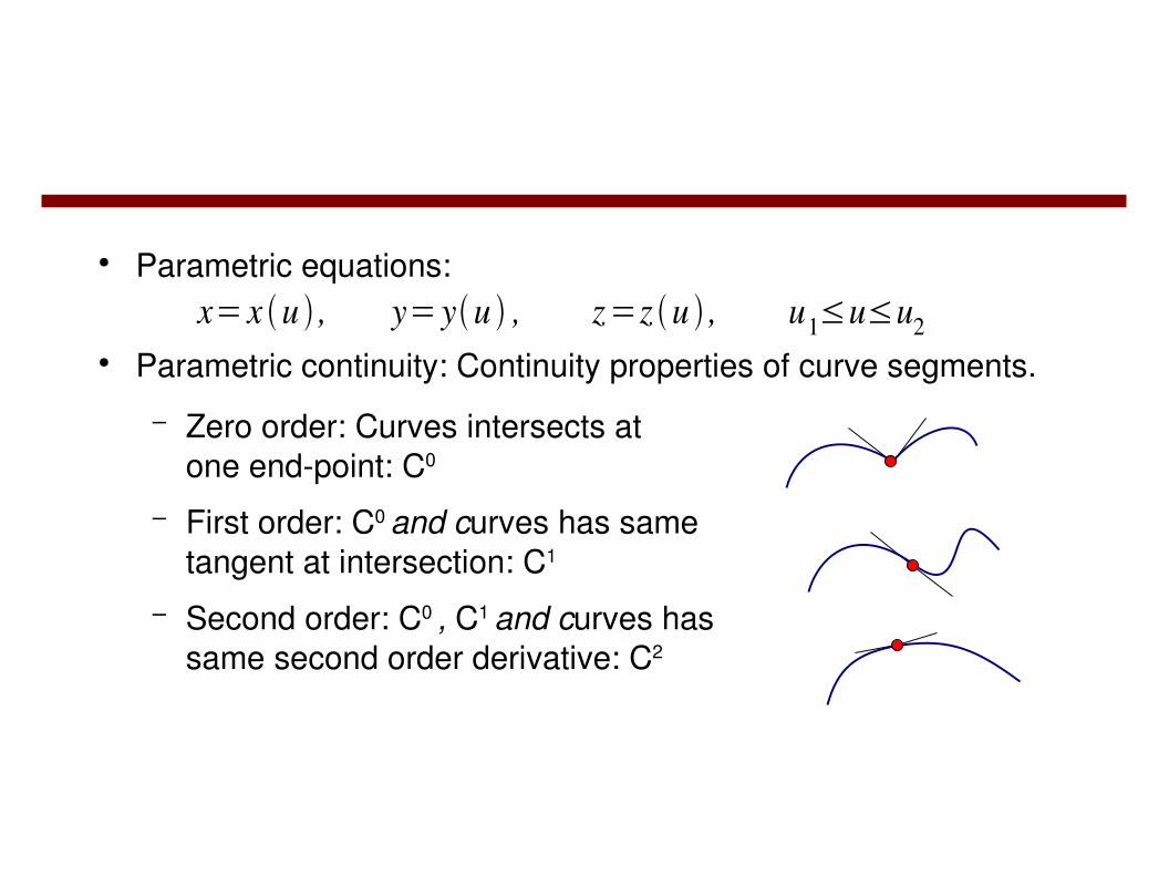
● Parametric equations:

● Parametric continuity: Continuity properties of curve segments.

– Zero order: Curves intersects at one end­point: C0 

– First order: C0 and curves has sametangent at intersection: C1 

– Second order: C0 , C1 and curves has same second order derivative: C2

x= x u ,        y= yu ,         z=z u ,         u1≤u≤u2

● Geometric continuity:Similar to parametric continuity but only the direction of derivatives are significant. For example derivative (1,2) and (3,6) are considered equal.

● G0, G1, G2 : zero order, first order, and second order geometric continuity.

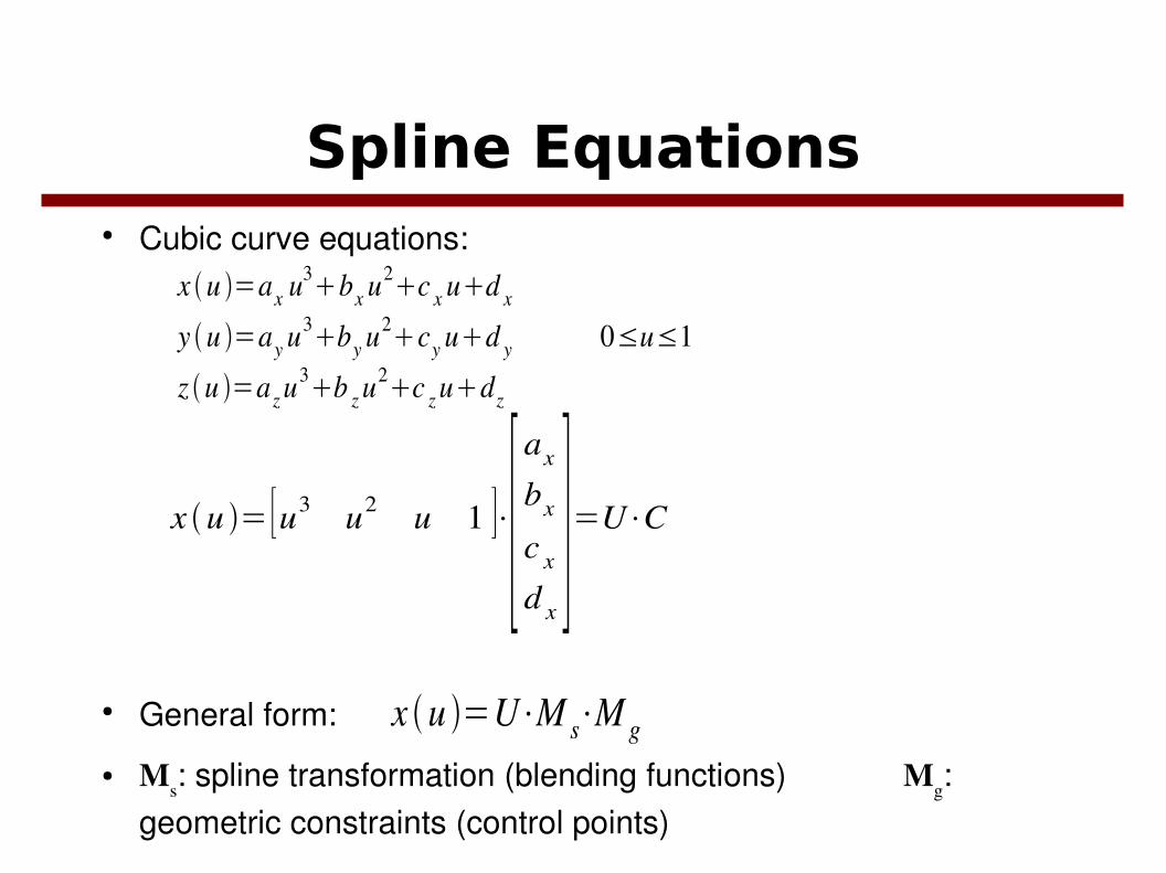
Spline Equations● Cubic curve equations:

● General form:

● Ms: spline transformation (blending functions)             Mg: geometric constraints (control points)

x u =ax u3bx u2

c x ud x

y u =ay u3by u2

cy ud y             0≤u≤1

z u =az u3b z u2

c z udz

x u = [u3 u2 u 1 ]⋅[ax

bx

c x

d x]=U⋅C

x u =U⋅M s⋅M g

Natural Cubic Splines● Interpolation of n+1 control points. n curve segments. 4n 

coefficients to determine ● Second order continuity. 4 equation for each of n­1 common 

points:

4n equations required, 4n­4 so far.● Starting point condition, end point condition.

● Assume second derivative 0 at end­points or add phantom control points p­1, pn+1.

x k1 =pk ,      x k1 0 =pk ,      { x k'1 = xk1

' 0 ,      { x ¿k

' '1 =x k1

' '0 ¿

x1 0 =p0 ,      x n 1 = pn

x1' '0 =0,      { xn

' '1 =0¿

● Write 4n equations for 4n unknown coefficients and solve.

● Changes are not local. A control point effects all equations.

● Expensive. Solve 4n system of equations for changes.

Hermite Interpolation● End point constraints for each segment is given as:

● Control point positions and first derivatives are given as constraints for each end­point.P 0 = pk ,          P 1 = pk1 ,           P 0 = pk ,          P 1= pk1 ,

P 0 =pk ,        P 1 =pk1 ,        { P'0 =Dpk ,        { P ¿

'1 =Dpk1 ,¿

P u =[u3 u2 u 1 ]⋅[abcd] P'

u =[3u2 2u 1 0 ]⋅[abcd]

[pk

pk1

Dpk

Dpk1]=[

0 0 0 11 1 1 10 0 1 03 2 1 0

]⋅[abcd] [

abcd]=[

0 0 0 11 1 1 10 0 1 03 2 1 0

]−1

⋅[pk

pk1

Dpk

Dpk1]

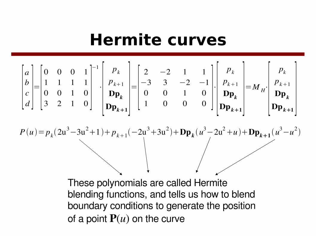
Hermite curves

[abcd]=[

0 0 0 11 1 1 10 0 1 03 2 1 0

]−1

⋅[pk

pk1

Dpk

Dpk1]=[

2 −2 1 1−3 3 −2 −10 0 1 01 0 0 0

]⋅[pk

pk1

Dpk

Dpk1]=M H⋅[

pk

pk1

Dpk

Dpk1]

P u =pk2u3−3u2

1 pk1−2u33u2

Dpk u3−2u2

u Dpk1 u3−u2

These polynomials are called Hermiteblending functions, and tells us how to blendboundary conditions to generate the positionof a point P(u) on the curve

Hermite blending functions

Hermite curves

● Segments are local. First order continuity● Slopes at control points are required.● Cardinal splines and Kochanek­Bartel splines approximate 

slopes from neighbor control points.

Bézier Curves

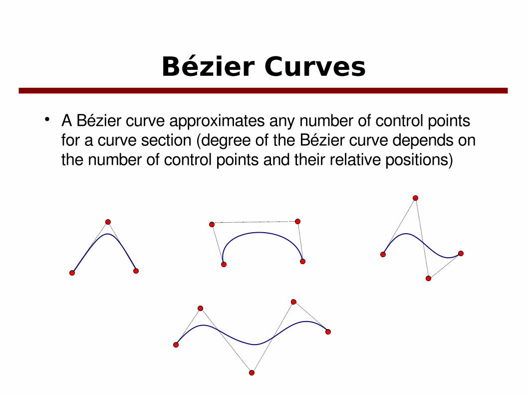
● A Bézier curve approximates any number of control points for a curve section (degree of the Bézier curve depends on the number of control points and their relative positions)

● The coordinates of the control points are blended using Bézier blending functions BEZk,n(u)

● Polynomial degree of a Bézier curve is one less than the number of control points.3 points : parabola4 points : cubic curve5 points : fourth order curve

P u =∑k=0

n

pk BEZk ,n u ,            0≤u≤1

BEZk , n u =nk u

k1−u n−k ,            nk =

n!k ! n−k !

Cubic Bézier Curves

● Most graphics packages provide Cubic Béziers.

BEZ0,3=1−u 3                      BEZ1,3=3u 1−u 2

BEZ2,3=3u21−u                  BEZ 3,3=u3

P u =[u3 u2 u 1 ]⋅M Bez⋅[p0

p1

p2

p3]

M Bez=[−1 3 −3 13 −6 3 0−3 3 0 01 0 0 0

]

Cubic Bézier blending functions

The four Bézier blending functions for cubic curves (n=3, i.e. 4 control pts.)

p0 p1

multiplied with

multiplied withmultiplied with

multiplied with

p2p3

Properties of Bézier curves

● Passes through start and end points

● First derivates at start and end are:

● Lies in the convex hull

P 0 =p0 ,             P 1 =pn

P'0 =−np0np1

P'1 =−npn−1npn

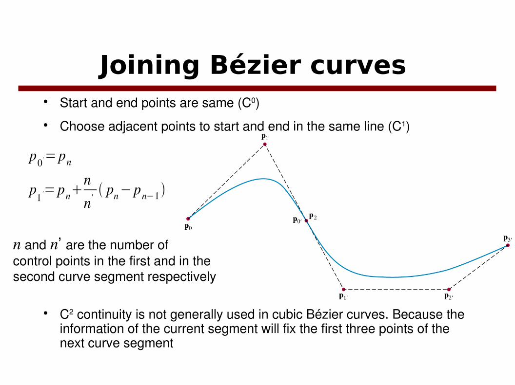
Joining Bézier curves ● Start and end points are same (C0)● Choose adjacent points to start and end in the same line (C1)

● C2 continuity is not generally used in cubic Bézier curves. Because the information of the current segment will fix the first three points of the next curve segment

p0'=pn

p1 '=pn

n

n' pn−pn−1

n and n’ are the number ofcontrol points in the first and in thesecond curve segment respectively

Bézier Surfaces

● Two sets of orthogonal Bézier curves are used.● Cartesian product of Bézier blending functions:

P u , v =∑j=0

m

∑k=0

n

p j , k BEZ j ,m v BEZ k ,n u           0≤u ,v≤1

Bézier Patches

● A common form of approximating larger surfaces by tiling with cubic Bézier patches. m=n=3

● 4 by 4 = 16 control points.

Cubic Bézier Surfaces

●  Matrix form

● Joining patches:similar to curves. C0, C1 can be established by choosing control points accordingly.

P u ,v =U⋅M Bez⋅P⋅M BezT⋅T T

=

[u3 u2 u 1 ]⋅[−1 3 −3 13 −6 3 0−3 3 0 01 0 0 0

]⋅[p0,0 p0,1 p0,2 p0,3

p1,0 p1,1 p1,2 p1,3

p2,0 p2,1 p2,2 p2,3

p3,0 p3,1 p3,2 p3,3]⋅[−1 3 −3 13 −6 3 0−3 3 0 01 0 0 0

]⋅[v3

v2

v1

]

Displaying Curves and Surfaces

● Horner's rule: less number of operations for calculating polynoms.

● Forward­difference calculations:Incremental calculation of  the next value.– Linear case and using subintervals of fixed size to divide 

u:

x u =ax u3bx u2

c x ud x

x u = ax ubx ucx ud x

uk1=ukδ ,           k=0,1,2, .. .            u0=0x k=a x ukb x              xk1=a xukδ bx

x k1=x k x             x=ax δ constant

Forward-difference for cubic-splines

● Cubic equations

x k=a x uk3b x uk

2c x ukd x          xk1=a xukδ

3b xukδ

2cx ukδ d x

xk=3a x uδ k23a x δ

22bx δ uk ax δ

3bx δ

2cx δ

xk1= xk 2 xk              2 xk=6a x δ2 uk6a x δ

32bx δ

2

2 x k1= 2 xk 3 x k          3 x k=6a x δ3

x 0=d x

x0=ax δ3bx δ

2c x δ

2 x 0=6a x δ32bx δ

2

Once we compute these initial values, the calculation for next x­coordinateposition takes only three additions.

Example

● Example:

(ax,bx,cx,dx)=(1,2,3,4), δ = 0.1

x x 2 x

4.000 0.321 0.0464.321 0.367 0.0524.688 0.419 0.0585.107 0.477 0.0645.584 0.541 0.0706.125 0.611 0.0766.736 0.687 0.0827.423 0.769 0.0888.192 0.857 0.0949.049 0.951 0.100

x 0=d x

x0=ax δ3bx δ

2c x δ

2 x 0=6a x δ32bx δ

2

3 xk=6a x δ3

3 xk=6⋅1⋅δ3=0 . 006

2

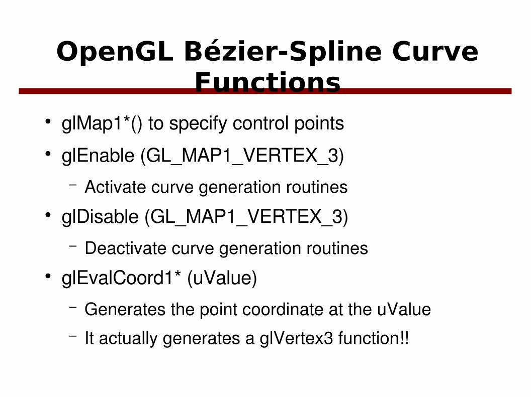
OpenGL Bézier-Spline Curve Functions

● glMap1*() to specify control points● glEnable (GL_MAP1_VERTEX_3)

– Activate curve generation routines● glDisable (GL_MAP1_VERTEX_3)

– Deactivate curve generation routines● glEvalCoord1* (uValue)

– Generates the point coordinate at the uValue– It actually generates a glVertex3 function!!

Example

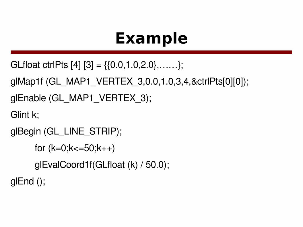
GLfloat ctrlPts [4] [3] = {{0.0,1.0,2.0},……};

glMap1f (GL_MAP1_VERTEX_3,0.0,1.0,3,4,&ctrlPts[0][0]);

glEnable (GL_MAP1_VERTEX_3);

Glint k;

glBegin (GL_LINE_STRIP);

for (k=0;k<=50;k++)

glEvalCoord1f(GLfloat (k) / 50.0);

glEnd ();

Generating uniformly spaced u values

  We may replace the glBegin(), inner for loop, and glEnd() with:

glMapGrid1f (50, 0.0, 1.0);

glEvalMesh1 (GL_LINE, 0, 50);

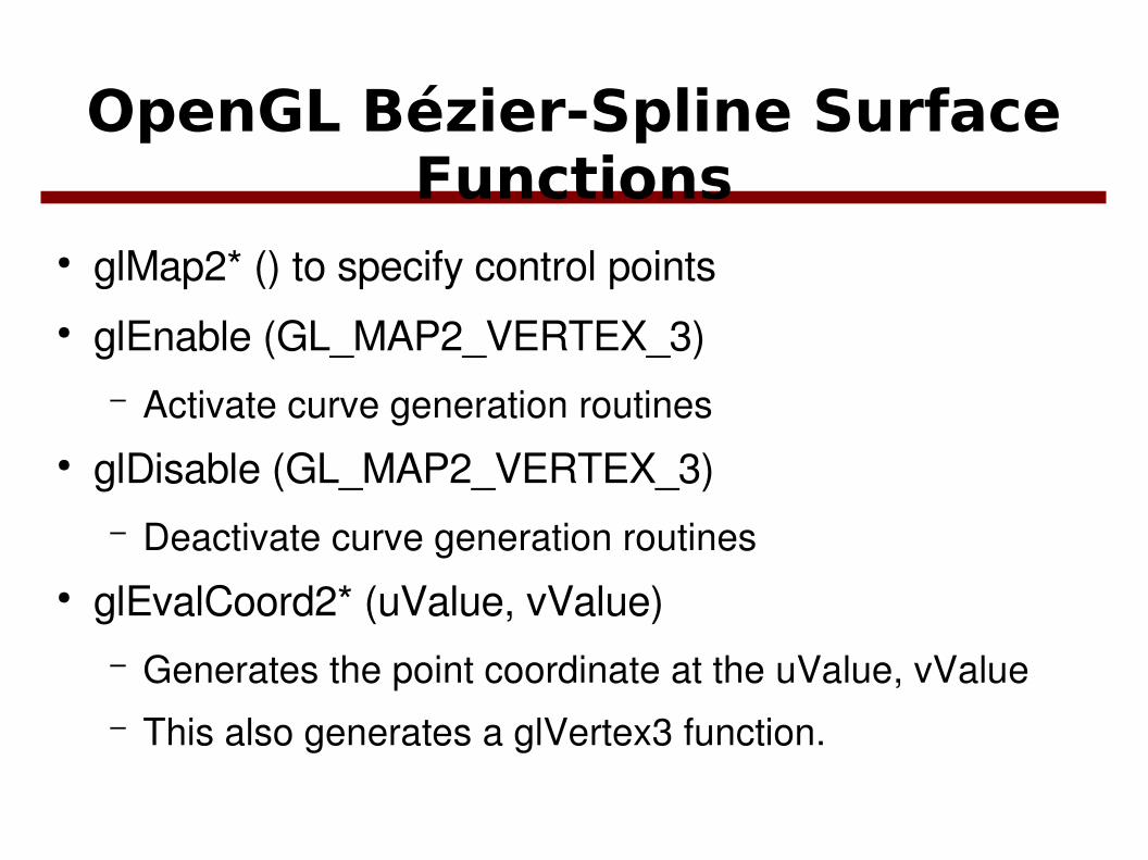
OpenGL Bézier-Spline Surface Functions

● glMap2* () to specify control points● glEnable (GL_MAP2_VERTEX_3)

– Activate curve generation routines● glDisable (GL_MAP2_VERTEX_3)

– Deactivate curve generation routines● glEvalCoord2* (uValue, vValue)

– Generates the point coordinate at the uValue, vValue– This also generates a glVertex3 function.

Example

GLfloat ctrlPts [4] [4] [3] = {{{0.0,1.0,2.0},……};

glMap2f (GL_MAP2_VERTEX_3,0.0,1.0,3,4,0.0,1.0,12,4,&ctrlPts[0][0][0]);

glEnable (GL_MAP2_VERTEX_3);

glMapGrid2f (40,0.0,1.0,40,0.0,1.0);

glEvalMesh2 (GL_LINE,0,40,0,40);

// GL_POINT and GL_FILL is also available with glEvalMesh2()

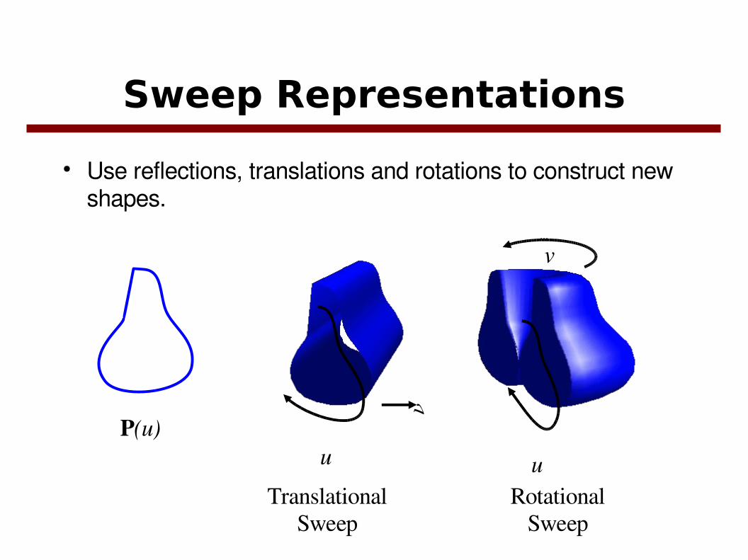
Sweep Representations

● Use reflections, translations and rotations to construct new shapes.

P(u)u

v

u

v

TranslationalSweep

RotationalSweep

Translational Sweep

Rotational Sweep

Hierarchical Models

● Combine smaller/simpler shapes to construct complex objects and scenes.

● Stored in trees or similar data structures● Operations are based on traversal of the tree ● Keeping information like bounding boxes in tree nodes 

accelarate the operations.

Scene Graphs

● DAG's (Directed Acyclic Graphs) to represent scenes and complex objects.

● Nodes: Grouping nodes, Transform nodes, Level Of Detail nodes, Light Source nodes, Attribute nodes, State nodes.Leaves: Object geometric descriptions.

● Why not tree but DAG?● Available libraries: i.e. www.openscenegraph.org

– Java3D is also based on Scene Graph Model● Efficient display of objects, picking objects, state change 

and animations.

Scene Graph Representation

G

TT

G

T

T

T T T T

T

G

T T

T T

L

Constructive Solid Geometry

● Combine multiple shapes with set operations (intersection, union, deletion) to construct new shapes.

A∪B A∩B A−B B−A

CSG Tree Representation

● Set operations and transformations combined:

● union(transA(box),diff(transB(box),transC(cylinder)))  

+

T

T

­

TA CSG Tree

● Ray casting methods are used for rendering and finding properties of  volumes constructed with this method.

● Parallel lines emanating from the xy plane (firing plane) along the z direction are intersected with the objects

● The intersection points are sorted according to the distance form the firing plane

● Based on the operation the extents (i.e., the surface limits) of the constructed object can be found.

Implementing CSG

Ray Casting

Ray Casting

● Simply +1 for outside→inside, ­1 for inside→outside transition. Positives are solid.

      A B C DP ∪ Q    1 2 1 0P ∩ Q    0 1 0 0P ­  Q    1 0   ­1 0Q ­  P   ­1 0 1 0

Implementation Details

RAY

PQ

A DCB

Calculating the Volume

Volume along the ray:

V ij≈ Aij zij

Total Volume:

V≈∑i , j

V ij

Octrees

● Divide a volume in equal binary partitions in all dimensions recursively to represent solid object volumes. Combining leaf cubes gives the volume.

● 2D: quadtree

1 2 3 41 2

3 4

● 2D: quadtree; 3D: octree● Volume data: Medical data like Magnetic Resonance.

Geographical info (minerals etc.)● 2D: Pixel ; 3D: voxel.● Volumes consisting of large continous subvolumes with 

properties. Volumes with many wholes, spaces. Surface information is not sufficient or tracktable.

● Keeping all volume in terms of voxels, too expensive: space and processor.– Therefore, homogeneous regions of the space can be 

represented by larger spatial components

● 8 elements at each node.● If volume completely resides in

a cube, it is not further divided:leaf node

● Otherwise nodes are recursivelysubdivided.

● Extent of a tree node is the extent of the cube it defines.● Surfaces can be extracted by traversing the leaves with 

geometrical adjacency.

01

32

45

7

6

Fractal Geometry Methods● Synthetic objects: regular, known dimension

● Natural objects: recursive (self repeating), the higher the precision, the higher the details you get.

● Example: tree branches, terrains, textures.

● Classification:

– Self­similar: same scaling parameter s is used in all dimensions, scaled­down shape is similar to original

– Self­affine: self similar with different scaling parameters and transformations. Statistical when random parameters are involved.

Fractal Dimension

● Fractal dimension:– Amount of variation of a self similar object. Denoted 

as D.– Fragmentation, roughness of the object.

● The fractal dimension of a self­similar fractal with a single scaling factor s is obtained using ideas from subdivision of a Euclidean object.

Fractal Dimension

The relationship between the number of subparts and the scaling factor is

n⋅sD E=1

where DE is the Euclidean dimension.

We can define the fractal dimensionsimilarly with number of subparts n and  a given scaling factor s.

n⋅sD=1

Koch curve

Initiator:

Generator:

The fractal dimension of the Koch curve

n sD=1

D=ln n

ln 1/ s

n: number of pieces s : scaling factor

n=4 s=1/3 D=ln 4

ln1/1/3=1.2619

Exercise

● What is the fractal dimension of the following shape?

Initiator Generator

Each edge of the square is replaced by the generator recursively.

What is n? What is s?  

Exercise

● What is the fractal dimension of the following shape?

Initiator Generator

Each edge of the square is replaced by the generator recursively.

n = 8,   s = 1/4,  D = 1.5  

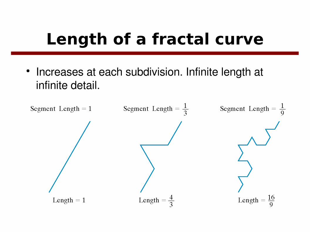
Length of a fractal curve

● Increases at each subdivision. Infinite length at infinite detail.

Random Variation● Using a probability 

distribution function we can introduce small variations during the subdivision of the object for more realism.

Images from a 1986 paper.

Random Mid-point Variation

● Find the midpoint of an edge A­B. Add a random factor and divide the edge in two as: A­M, M­A at each step.

● Usefull for height maps, clouds, plants.● 2D:

● 3D:  For corners of a square: A, B, C, D

A B

CD

M

x m= x A xB /2ym= y AyB /2r

r is a random number selectedfrom Gaussian distribution withmean 0 and variance that depends on Dand the length between end points

Z AB= Z AZ B/2r ,           Z BC= Z BZ C /2r ,ZCD=Z CZ D/2r ,           Z DA= Z DZ A/2r ,Z M= Z ABZ BCZ CDZ DA /4r ,

Random Mid-point Variation