3D model-based tracking with one omnidirectional camera ...
102
POLITECNICO DI MILANO Corso di Laurea in Ingegneria Informatica Dipartimento di Elettronica e Informazione 3D model-based tracking with one omnidirectional camera and particle filters. AI & R Lab Laboratorio di Intelligenza Artificiale e Robotica del Politecnico di Milano Relatore: Prof. Matteo Matteucci Correlatore Esterno: Prof. Alexandre Bernardino Tesi di Laurea di: Matteo Taiana, matricola 633410 Anno Accademico 2006-2007
Transcript of 3D model-based tracking with one omnidirectional camera ...

POLITECNICO DI MILANOCorso di Laurea in Ingegneria InformaticaDipartimento di Elettronica e Informazione
3D model-based tracking with one
omnidirectional camera and particle
filters.
AI & R Lab
Laboratorio di Intelligenza Artificiale
e Robotica del Politecnico di Milano
Relatore: Prof. Matteo Matteucci
Correlatore Esterno: Prof. Alexandre Bernardino
Tesi di Laurea di:
Matteo Taiana, matricola 633410
Anno Accademico 2006-2007


Alla mia famiglia:i miei nonni,
i miei genitori,mia sorella
e il mio cagnolino.


Abstract
In order to carry out complex tasks robots need to extract informationfrom the environment they operate in. Vision is probably the richest sensoremployed in current robotic systems, due to the possibility of measuring agreat diversity of features in the environment, e.g., colors, distances, texturesand shapes. Omnidirectional vision cameras provide the additional benefitof an enlarged field of view.
In the context of semi-structured scenarios, as is the example of theRoboCup Middle Size League, the particular nature of the objects and theirmotions can be exploited to allow computer vision methods to work reliablyand in real-time: objects are known to have specific colors and shapes, andmotion follows the laws of physics. Color, shape and motion will be used inthis thesis to develop a robust 3D object tracking system for autonomousrobots equipped with one dioptric or catadioptric omnidirectional camera.
This thesis addresses three main problems in the context of 3D objecttracking: (i) how to relate object’s 3D shape and position information withthe acquired 2D images; (ii) how to obtain measurements from the imagestaking into account the colors of objects and background; and (iii) how tointegrate temporal information taking into account the laws of physics. Weshow that Particle Filtering methods constitute an adequate framework foraddressing consistently all these problems.
The proposed architecture provides an efficient and reliable methodol-ogy to perform 3D target tracking for robots equipped with one omnidirec-tional camera. The accuracy and precision of the algorithm were tested in aRoboCup Middle Size League scenario, with static and moving targets, us-ing either a catadioptric or a dioptric omnidirectional camera. The real-timecapabilities of the system were also evaluated.
As a result of this work two papers were accepted in refereed internationalconferences: [38] and [39].
I

Acknowledgments
I would like to thank my main advisor, Prof. Alexandre Bernardino for hisfriendship and guidance, for making me feel at home form the very beginningin Portugal and at Instituto Superior Tecnico.
I want to thank my other three advisors for the confidence they placed inme: Prof. Pedro Lima from Instituto Superior Tecnico, Prof. Matteo Mat-teucci and Prof. Andrea Bonarini from Politecnico di Milano. I am gratefulto Prof. Jose Gaspar, Dr Jacinto Nascimento and Abdolkarim Pahliani forthe fruitful collaboration.
I would like to thank the friends who helped me throughout the workof this thesis, especially Dr Alessio Del Bue, Dr Luis Montesano and HugoCostelha. I also wish to thank the lots of friends who supported me fromthe three different laboratories I belonged to: AIRLab, ISLab and VisLab.
Finally, I would like to thank all the friends who roamed with me thecorridors of Politecnico, playing minella/studying. Your friendship is themost valuable outcome of those past years.
III


Riassunto
0.1 Introduzione
I robot sono sistemi controllati elettronicamente, in grado di interagire at-traverso percezione e azione col mondo che li circonda; usano sensori peracquisire informazioni sull’ambiente e attuatori per compiere azioni. I robotsono definiti autonomi quando possono svolgere gli incarichi che sono loroassegnati senza la necessita di un intervento umano.
Una classe di sensori comunemente impiegata nella robotica, tipicamentecon compiti di autolocalizzazione e navigazione, e quella delle telecamereomnidirezionali, cioe telecamere che hanno una ampiezza di campo visivomolto grande. Il vantaggio di questo tipo di telecamera, rispetto a quelleconvenzionali, con funzione di proiezione prospettica, e quello di acquisireinformazioni su una porzione maggiore dello spazio che circonda il robot. Letelecamere proiettano i raggi di luce provenienti dall’ambiente su un sensoredi immagine, un piano di celle CCD o CMOS. Esso converte l’informazioneluminosa in cariche elettriche, formando l’immagine digitale. A secondadella modalita con la quale la luce e proiettata sul sensore di immagine,le telecamere sono classificate come diottriche (quelle per cui la proiezioneavviene solo tramite diffrazione) o catadiottriche (quelle per cui la proiezioneavviene tramite riflessione e diffrazione). Uno svantaggio delle telecamereomnidirezionali rispetto alle convenzionali sta nel fatto che le immagini cheproducono sono soggette a forte distorsione, questo puo costringere all’usodi algoritmi non standard per l’identificazione e l’inseguimento di oggetti.Un altro problema particolarmente evidente nel tracking con telecamere om-nidirezionali e che l’oggetto inseguito, immerso in una scena dinamica, puopresentare nell’immagine occlusioni, sovrapposizioni e, in generale, ambi-guita.
Questa tesi presenta un sistema di inseguimento 3D basato su particlefilter, per robot autonomi equipaggiati con telecamere omnidirezionali. Ilsistema di inseguimento e progettato per funzionare in un ambiente parzial-
V

mente strutturato, in cui ogni oggetto abbia un proprio colore distintivo, manel quale l’illuminazione sia variabile, come quello della RoboCup MiddleSize League (MSL). Le ipotesi del filtro rappresentano posizione e velocitatridimensionali dell’oggetto inseguito, la funzione di verosimiglianza si basasu colore e forma dell’oggetto.
0.2 Descrizione del sistema
Abbiamo progettato e implementato un sistema di inseguimento robusto perrobot autonomi equipaggiati con una telecamera omnidirezionale, diottricaoppure catadiottrica.
Usiamo un particle filter per stimare a ogni istante la posizione e la ve-locita tridimensionali di un oggetto, date le osservazioni prese negli istanti ditempo precedenti e una funzione di densita di probabilita iniziale. In questatesi consideriamo solo oggetti rotazionalmente simmetrici, ma il metodo puoessere facilmente esteso perche funzioni con oggetti rigidi di forma arbitraria,includendo la stima sull’orientazione e la velocita di rotazione.
I particle filters usano una rappresentazione basata su campioni dellafunzione di densita di probabilita; ogni campione e chiamato particella op-pure ipotesi. Per calcolare iterativamente la stima di posizione e velocitadell’oggetto inseguito, e necessario modellare probabilisticamente sia la suadinamica di moto che la maniera in cui calcoliamo la verosimiglianza di unaparticella.
Per calcolare l’approssimazione della funzione di densita di probabilita aposteriori, gli algoritmi di inseguimento funzionano tipicamente in tre passi:
1. Previsione - calcola una approssimazione di p(xt | y1:t−1) , muovendoogni particella come indicato dal modello di movimento;
2. Aggiornamento - il peso di ogni particella i e aggiornato usando laverosimiglianza p(yt | x(i)
t ):
w(i)t ∝ w
(i)t−1p(yt | x(i)
t ) (1)
3. Resampling (ricampionamento) - le particelle con un peso alto sonoreplicate, mentre quelle con un peso basso sono dimenticate.
Per caratterizzare la dinamica dell’oggetto usiamo un modello autore-gressivo a velocita costante: a ogni istante di tempo la velocita delle parti-celle e aggiornata sommando a essa un rumore di accelerazione. La posizionedelle particelle e aggiornata, in funzione della velocita che le caratterizzavanell’istante precedente e dell’accelerazione.

Abbiamo progettato un modello di osservazione per associare un valoredi verosimiglianza a una posizione ipotetica, dato il modello dell’oggettoinseguito, una immagine acquisita dalla telecamera omnidirezionale e il cor-rispondente modello di proiezione della telecamera.
Nel corso del lavoro usiamo due telecamere omnidirezionali: una cata-diottrica (si veda la Figura 1a) e una diottrica (si veda la Figura 2a). Latelecamera catadiottrica e costituita da una telecamera prospettica di frontealla quale e posto uno specchio, il cui profilo e stato progettato perche il sis-tema finale produca una vista a risoluzione costante del pavimento. Permodellare esattamente questa telecamera sarebbe necessario usare un gene-rico Catadioptric Projection Model (CPM) (Figura 1b), che tiene conto dellospecifico profilo dello specchio. Dato che questo modello esatto e non linearee non e esprimibile in forma chiusa, usiamo due modelli di proiezione ap-prossimati: lo Unified Projection Model (UPM) (Figura 1c) e il PerspectiveProjection Model (PPM), che e un caso particolare dell’UPM. La telecameraomnidirezionale diottrica (fish-eye) e semplicemente una telecamera con unalente fish-eye, che le conferisce un’apertura di campo di 185◦. Per modellarlausiamo l’Equidistance Projection Model (EPM) (Figura 2b).
Ognuno dei modelli di proiezione impiegato deve essere calibrato (si vedala Figura 3) prima di essere usato. I valori dei suoi parametri sono ottenutiminimizzando l’errore di backprojection. Vengono effettuate due proiezionidi un insieme di punti tridimensionali sull’immagine, una prioeizione e fattafisicamente, usando la telecamera, mentre l’altra e effettuata tramite il mo-dello. L’errore di backprojection e semplicemente la media quadratica delledistanze tra i punti proiettati con i due sistemi.
Gli oggetti inseguiti dal sistema sono caratterizzati dalla propria formatridimensionale, dalla dimesione e dal colore. Modelliamo la forma tridi-mensionale degli oggetti con forme geometriche semplificate, mentre il lorocolore e modellato con un istogramma di colore, il quale e costruito in unafase di impostazione del sistema, anteriore al tracking. L’istogramma dicolore e costruito basandosi su alcune proiezioni dell’oggetto sull’immagine,acquisite in condizioni di illuminazione e posizioni diverse.
I passi per associare un valore di verosimiglianza a una ipotesi sono:
• Proiezione del modello di forma tridimensionale sul piano dell’imma-gine. Il risultato sono due insiemi di pixel, uno su ciascun lato delcontorno che l’oggetto seguito proietterebbe se si trovasse esattamentenella posizione ipotetica.
Per ottenere i due insiemi di pixel, il modello della forma e traslato eruotato affinche si trovi nella posizione ipotetica. La rotazione e resa

F(t)
f
P=(r,z)
z
r
t
q
f
r
(a) (b)
(c)
Figure 1: (a) Telecamera omnidirezionale catadiottrica. (b) Il generico modello di
proiezione catadiottrico: Catadioptric Projection Model. (c) Il modello di proiezione
per telecamere centrali: Unified Projection Model.

(a) (b)
Figure 2: (a) Telecamera omnidirezionale diottrica, si noti la lente fisheye. (b) Il modello
di proiezione Equidistance Projection Model.
(a) (b)
Figure 3: (a) Immagine usata per la calibrazione. (b) Risultato della calibrazione: punti
proiettati dalla telecamera (croci blu), punti proiettati usando il modello di proiezione
non calibrato (cerchi verdi) e usando il modello con i valori dei parametri ottenuti con
la calibrazione (cerchi rossi) - le frecce indicano l’effetto della calibrazione su quattro
punti.

necessaria dal fatto che usiamo un modello semplificato della forma3D, il quale ci permette di proiettare solo i punti 3D che andranno aformare il contorno della proiezione dell’oggetto.
Per determinare i due insiemi di pixel usiamo uno di due metodi: ilprimo metodo e basato sulle B-spline e su distanze misurate nell’im-magine, mentre l’altro indivua in 3D i punti che verranno proiettatiall’interno e all’esterno del contorno ipotetico (si veda il Capitolo 4per i dettagli sui due metodi).
La proiezione dei punti tridimensionali verso i punti bidimensionalidell’immagine avviene attraverso l’applicazione del modello di proie-zione scelto.
• Costruzione di due istogrammi di colore, che caratterizzano il coloredell’immagine nell’intorno interno ed esterno del contorno proiettato.
Usiamo istogrammi nello spazio colore HSI (Hue, Saturation, Inten-sity) con 12 × 12 × 4 bin nell’implementazione Matlab. Nell’imple-mentazione C++, invece, usiamo lo spazio colore YUV e 4 × 8 × 8bin. In entrambi i casi usiamo un numero di bin per il canale checodifica l’informazione sull’intensita luminosa minore del numero deibin usati per codificare l’informazione degli altri canali. Questa sceltaserve a conferire robustezza al sistema rispetto ai cambiamenti di il-luminazione. Trascurare completamente l’informazione sull’intensitaluminosa ci avrebbe impedito di inseguire oggetti bianchi o neri.
• Calcolo della verosimiglianza in funzione della similarita tra coppie diistogrammi di colore.
Calcoliamo la similarita tra due istogrammi con la metrica di Bhat-tacharyya. Maggiore la similarita tra l’istogramma che modella l’og-getto da inseguire e quello che descrive il colore dell’immagine all’in-terno del contorno proiettato, maggiore la verosimiglianza dell’ipotesi.Minore la similarita tra i due istogrammi che descrivono il coloredell’immagine ai due lati del contorno proiettato, maggiore la vero-simiglianza. La prima di queste due regole in pratica significa cheassociamo una verosimiglianza alta a contorni che hanno al loro in-terno colori simili a quello dell’oggetto inseguito. La seconda significache associamo una alta verosimiglianza a contorni nel cui intorno sitrova una transizione cromatica (o di luminosita). Usiamo un coeffi-ciente per pesare l’influenza delle due regole sulla funzione di verosi-miglianza. Nella Figura 4 sono rappresentati i contorni proiettati dauna palla, in tre diverse posizioni ipotetiche, su un’immagine acquisita

Figure 4: Tre contorni ipotetici proiettati sull’immagine. In questa discussione in-
dichiamo per bervita con: “colore all’interno (o all’esterno) di un contorno” il co-
lore all’interno (o all’esterno) del contorno, in prossimita dello stesso. Il contorno A
ha una bassa verosimiglianza, a causa della grande differenza tra il modello di colore
dell’oggetto e il colore all’interno del contorno (il colore all’interno del contorno non e
arancione) e una grande similarita tra il colore ai due lati del del contorno. Il contorno
C e associato con una verosimiglianza media, perche il modello di colore dell’oggetto e
il colore all’interno del contorno sono simili, ma i colori ai due lati del contorno sono
simili. Il contorno B ha una alta verosimiglianza, in quanto il colore all’interno del
contorno e simile al modello di colore della palla e i colori ai due lati del contorno sono
diversi.
col sistema catadiottrico. Viene mostrato come la funzione di verosi-miglianza privilegi l’ipotesi col contorno piu simile a quello della pallapresente nell’immagine. Questo metodo, comparato con altri che sibasano sulla estrazione dei contorni, e piu robousto dato che riesce agestire anche contorni sfumati, che sono frequenti negli ambienti di-namici.
Per inizializzare il particle filter usiamo due metodi: (i) impostiamo lafunzione di densita di probabilita iniziale secondo una Gaussiana con un’altavarianza, centrata su una stima fatta a mano della posizione e velocita ini-ziale dell’oggetto inseguito, oppure (ii) selezioniamo una posizione tridimen-sionale in base a una identificazione bidimensionale dell’oggetto e usiamoquesta come come media della Gaussiana (si veda il Capitolo 5 per maggioriinformazioni).
0.3 Risultati sperimentali e direzioni di ricerca
Abbiamo sviluppato sia un’implementazione del sistema in Matlab, che unain C++ basata sulla libreria Integrated Performance Primitives (IPP) dellaIntel. Abbiamo eseguito diversi esperimenti, nell’ambiente della RoboCupMSL, per verificare l’accuratezza e la precisione del sistema di inseguimentoproposto.
Abbiamo eseguito diversi inseguimenti su sequenze di immagini acquisitecon la telecamera omnidirezionale catadiottrica. Usando il modello di pro-iezione UPM, abbiamo inseguito una palla in una sequenza di immaginiin cui essa scendeva lungo una rampa, una palla lungo una traiettoria concambiamenti repentini della direzione di moto (rimbalzi sul campo), si vedala Figura 5 e un robot lungo una traiettoria sul pavimento. Gli insegui-menti della palla mostrano la robustezza del metodo rispetto a motion blure rumore del sensore di immagine (Figura 6a e 6b).
Sempre nella configurazione con telecamera catadiottrica, abbiamo ese-guito un esperimento per misurare l’accuratezza del sistema proposto: abbi-amo posto una palla in diverse posizioni attorno al robot e misurato l’errorenella localizzazione ottenuta col nostro metodo, rispetto alla posizione reale.
Abbiamo comparato i risultati di inseguimento e localizzazione ottenutiusando due diversi modelli del sensore catadiottrico, UPM e PPM, verifi-cando che PPM fornisce prestazioni simili a UPM per accuratezza e preci-sione, ma offre il vantaggio di un costo computazionale meno elevato.
Abbiamo inoltre inseguito una palla in una sequenza di immagini ac-quisita con la configurazione diottrica del sensore omnidirezionale, verifi-cando la robustezza del sistema contro le occlusioni (si veda la Figura 6c) ela sua capacita di funzionare in tempo reale (29fps su un processore Pentium4 a 2.6GHz).
In futuro intendiamo estendere il sistema rendendolo in grado di inseguirepiu oggetti contemporaneamente. Vogliamo sperimentare l’uso di modelli dimovimento multipli, per esempio uno che descriva il moto di una palla cherotola liberamente sul pavimento e un altro che descriva il comportamentodella palla in presenza di un urto. Intendiamo inoltre sfruttare la carat-teristica del sistema di avere un vettore di stato con le coordinate spazialidell’oggetto inseguito, usando modelli di movimento basati sulle leggi dellafisica (per esempio applicando l’accelerazione di gravita agli oggetti che nonsono in contatto con il suolo). Esprimeremo le coordinate dell’oggetto inun sistema di riferimento inerziale. Per far questo useremo la ego-motioncompensation: applicheremo il movimento effettuato dal robot, al contrario,sulle particelle del filtro.

(a)
(b)
Figure 5: (a) Palla che scende lungo una rampa: i dieci percorsi risultanti da dieci
esecuzioni dell’algoritmo sulla stessa sequenza di immagini. Le dieci linee blu con
punti rossi rappresentano le dieci traiettorie tridimensionali stimate, le linee blu sono
le proiezioni di queste traiettorie sul piano di terra e su quello laterale. (b) Palla
rimbalzante: stesso tipo di grafico per le traiettorie stimate nella sequenza di immagini
nella quale la palla rimbalza sul pavimento.

(a) (b) (c)
Figure 6: Ingrandimenti di alcune immagini in cui il sistema di seguimento ha successo
nonostante condizioni poco favorevoli. (a) Un’immagine che presenta del motion blur
sulla proiezione della palla. (b) Un’immagine in cui e evidente il rumore del sensore di
immagine. (c) Un’immagine in cui la palla e visibile solo in parte, a causa dell’occlusione
da parte di un robot.


Contents
Abstract I
Acknowledgments III
Riassunto V0.1 Introduzione . . . . . . . . . . . . . . . . . . . . . . . . . . . . V0.2 Descrizione del sistema . . . . . . . . . . . . . . . . . . . . . . VI0.3 Risultati sperimentali e direzioni di ricerca . . . . . . . . . . . XII
1 Introduction 11.1 Problem formulation . . . . . . . . . . . . . . . . . . . . . . . 11.2 Description of the system . . . . . . . . . . . . . . . . . . . . 31.3 Structure of the thesis . . . . . . . . . . . . . . . . . . . . . . 5
2 State of the art 72.1 Color based image measurements . . . . . . . . . . . . . . . . 72.2 Tracking . . . . . . . . . . . . . . . . . . . . . . . . . . . . . . 82.3 3D model based methods . . . . . . . . . . . . . . . . . . . . 9
3 Omnidirectional vision 113.1 Catadioptric omnidirectional camera . . . . . . . . . . . . . . 11
3.1.1 Projection models . . . . . . . . . . . . . . . . . . . . 133.2 Dioptric omnidirectional camera . . . . . . . . . . . . . . . . 14
4 Model-based detection in omnidirectional images 194.1 Detection algorithm . . . . . . . . . . . . . . . . . . . . . . . 194.2 3D model . . . . . . . . . . . . . . . . . . . . . . . . . . . . . 20
4.2.1 Selection of boundary pixels using sampling . . . . . . 234.2.2 Selection of boundary pixels using B-splines . . . . . . 23
4.3 Color model . . . . . . . . . . . . . . . . . . . . . . . . . . . . 264.4 Likelihood . . . . . . . . . . . . . . . . . . . . . . . . . . . . . 30
XVII

5 Tracking with particle filters 335.1 Particle filter tracking. . . . . . . . . . . . . . . . . . . . . . . 33
5.1.1 Motion model . . . . . . . . . . . . . . . . . . . . . . . 355.1.2 Observation model . . . . . . . . . . . . . . . . . . . . 35
5.2 Initialization of the particle filter . . . . . . . . . . . . . . . . 35
6 Experimental results 376.1 Catadioptric setup, UPM . . . . . . . . . . . . . . . . . . . . 37
6.1.1 Ball tracking . . . . . . . . . . . . . . . . . . . . . . . 386.1.2 Robot tracking . . . . . . . . . . . . . . . . . . . . . . 386.1.3 Error evaluation . . . . . . . . . . . . . . . . . . . . . 40
6.2 Catadioptric setup, UPM and PPM experimental comparison 436.2.1 Error evaluation . . . . . . . . . . . . . . . . . . . . . 436.2.2 Ball tracking . . . . . . . . . . . . . . . . . . . . . . . 46
6.3 Dioptric setup . . . . . . . . . . . . . . . . . . . . . . . . . . . 476.3.1 Jumping ball . . . . . . . . . . . . . . . . . . . . . . . 476.3.2 Occlusions . . . . . . . . . . . . . . . . . . . . . . . . . 486.3.3 Multiple objects . . . . . . . . . . . . . . . . . . . . . 48
7 Conclusions and future work 59
Bibliography 61
A Paper published in RoboCup Symposium 2007 65
B Paper to be published in IROS 2007 79

Chapter 1
Introduction
“Though the ether is filled with vibrations the world is in dark.
But one day man opens his seeing eye, and there is light.”
Ludwig Wittgenstein
1.1 Problem formulation
Robots are computer-controlled devices capable of perceiving and manipu-lating the physical world [40]. They use sensors to acquire information onthe environment and actuators to perform actions. Autonomous robots aremachines which can accomplish tasks without direct human intervention [1].
One class of sensors which is commonly used in robotics, especially fortasks such as self localization and navigation [30],[16], is that of omnidirec-tional cameras i.e., cameras characterized by a very wide field of view [19].Their main advantage over conventional, perspective cameras is that the firstgather information from a lager portion of the space surrounding a robot.Cameras project light rays radiating from the environment onto the imagesensor, a plane of CCD or CMOS cells, which in turn converts this infor-mation to electrical charges, forming the digital image. Depending on theway light is projected onto the image sensor, omnidirectional cameras areclassified either as dioptric (those in which projection is performed solely bymeans of refraction) or catadioptric (those in which projection is performedby combined reflexion and refraction). One drawback which is common toomnidirectional cameras is that the images they produce are affected bystrong distortion and perspective effects, which may lead to the use of non-standard algorithm for object detection and tracking. Another difficultythat affects tracking under these conditions is that the object of interest,

2 Chapter 1. Introduction
embedded in a dynamic scenario, may suffer from occlusion, overlap andambiguities.
This thesis presents a 3D particle-filter [40, 13] (PF) tracker for au-tonomous robots equipped with omnidirectional cameras. The tracker isdesigned to work in a structured, color-coded environment such as theRoboCup Middle Size League (MSL). The particles of the filter represent3D positions and velocities of the target, the likelihood function is basedon the color and shape of the target. From one image frame to the next,the particles are moved according to an appropriate motion model. Then,for each particle, a likelihood is computed, in order to estimate the objectstate. To calculate the likelihood of a particle we first project the contourof the object it represents on the image plane (as a function of the object3D shape and position) using a model for the omnidirectional vision system.The likelihood is then calculated as a function of three color histograms: onerepresents the object color model and is computed in a training phase withseveral examples taken from distinct locations and illumination conditions;the other two histograms represent the inner and outer boundaries of theprojected contour, and are computed at every frame for all particles. Theidea is to assign a high likelihood to the contours for which the inner pixelshave a color similar to the object, and are sufficiently distinct from outsideones.
A work closely related to this is described in [32], although in that casethe tracking is accomplished on the image plane. Tracking the position of anobject in 3D space instead of on the image plane has two main advantages:(i) the motion model used by the tracker can be the actual motion modelof the object, while in image tracking the motion model should describemovements of the projection of the object on the image plane and, becauseof the aforementioned distortion, a good model can be difficult to formulateand use; (ii) with 3D tracking the actual position of the tracked object isdirectly available, while a further non-trivial step is needed for a systembased on an image tracker to provide it.
During the work for this thesis we developed both a Matlab and a C++implementation of the tracker. The C++ implementation is based on vectorand matrix operations provided by the IPP library by Intel. It was developedto assess the real-time capabilities of the method.
We ran several experiments, in a RoboCup MSL scenario, to assess theaccuracy and precision of the proposed tracking method with color-codedobjects. We tested the two implementations with either a dioptric or cata-dioptric omnidirectional camera and different projection models for the lat-ter. We tracked a ball along movements in the 3D space surrounding the

1.2. Description of the system 3
robot, assessing the robustness of the method against occlusions and illumi-nation changes. We tracked a robot maneuvering. We ran an experimentplacing a still ball at different positions around the robot and measuringthe error of the detected position with respect to the ground truth. Wefurthermore compared the results obtained in the tracking and detection,using two different models for the catadioptric sensor.
In future work we intend to extend the system with the ability to trackmultiple objects. We will introduce the use of multiple motion models, forexample use a model describing the motion of a ball rolling freely and an-other describing the motion of a ball bouncing against an obstacle. We alsointend to use physics-based motion models (e.g., applying gravitational ac-celeration to particles which model flying balls). We will express the target’scoordinates in an inertial reference frame, instead of the robot-centered onewe use now. This will be combined with ego-motion compensation: applyingthe inverse motion of the robot to the filter’s particles. We also plan to testthe tracker in a non-color-coded environment.
1.2 Description of the system
We designed and implemented a robust 3D tracking system for autonomousrobots equipped with an omnidirectional, dioptric or catadioptric camera.
We use a particle filter to estimate at each time step the 3D position andvelocity of a target, given the observations taken in the previous time stepsand an initial probability density function (pdf). In this thesis we consideronly targets which are rotationally symmetric, but the method can be easilyextended to work with arbitrary rigid objects, including the estimate of theobject’s orientation.
PF’s use sample-based representations of pdf’s in which each sampleis called a particle or an hypothesis. To iteratively compute the estimateon the target’s position, one has to model probabilistically both its motiondynamics and the way we compute the likelihood of a particle.
For the motion dynamics we use a constant velocity autoregressive model:at each time step the velocity of the particles is updated by adding an accel-eration disturbance to it. The position of the particles is updated, accordingto the velocity of the previous time step and the acceleration disturbance.
We designed an observation model to associate a likelihood to an hypo-thetical position, given the model of the tracked object, one image acquiredwith an omnidirectional camera and the corresponding, calibrated projec-tion model for the camera.

4 Chapter 1. Introduction
The tracked objects are characterized by their 3D shape, size and color.We characterize the 3D shape of the objects with simplified geometric shapesand describe their color with a color histogram, which is built in a trainingphase with several examples taken from distinct locations and illuminationconditions.
The steps to compute the likelihood of an hypothesis are:
• Projection of the target model onto the image plane, resulting in twopixel sets, one on each side of the contour projected by the hypotheticaltarget.
To obtain the two pixel sets, the object shape model is shifted androtated to the hypothetical 3D position and projected onto the image(see Chapter 4 for details on the two alternative methods we use). Therotation of the model is needed because we use a simplified model forthe shape, that allows us to projet only the 3D points which will resultin the contour of the projection of the object.
The projection of 3D points to 2D image points is done with a modelfor the omnidirectional camera in use. In this work we acquire imagesusing a dioptric (fish-eye) or a catadioptric omnidirectional camera.We model the dioptric camera with the Equidistance Projection Model(EPM) and the catadioptric camera with either the Unified Projec-tion Model (UPM) or the Perspective Projection Model (PPM). Eachmodel has to be calibrated before being used.
• Building of two color histograms, characterizing the color in the imageon the boundaries of the projected contour.
• Calculation of the likelihood as a function of the similarity betweencolor histograms.
We compute the similarity between couples of histograms, with theBhattacharyya similarity metrics, as in [33]. The higher the similaritybetween the target model histogram and the histogram describing thecolor on the inside of the projected contour, the higher the likelihood.The lower the similarity between the two histogram describing thecolor on the two sides of the contour, the higher the likelihood.
To initialize the particles for the PF we either use a Gaussian distribu-tion with large variance, centered at rough estimates of the object’s initialposition and velocity or select a position in 3D space, based on a 2D detec-tion of the object, and use that as center for the Gaussian (see Chapter 5for details).

1.3. Structure of the thesis 5
1.3 Structure of the thesis
In Chapter 2 we describe the state of the art. In Chapter 3 we present ouromnidirectional sensors and introduce the models we use for their projec-tions. In Chapter 4 we delineate how the model-based detection of objectsin omnidirectional images is performed. In Chapter 5 we detail our PF-based tracking algorithm. In Chapter 6 we present the experimental resultsobtained, while in Chapter 7 we draw conclusions and present future devel-opments of this work.

6 Chapter 1. Introduction

Chapter 2
State of the art
“Our knowledge can be only finite,
while our ignorance must necessarily be infinite.”
Karl Popper
This thesis addresses the object tracking problem in a semi-structured en-vironment using an omnidirectional camera. The environment considered isthe one of the RoboCup Middle Size League, where objects have particularshapes and colors but the illumination conditions can be diverse, and occlu-sions/ambiguities are frequent. In this chapter we will describe the currentstate of the art in the several topics this thesis addresses for achieving theproposed goals: (i) the image measurement methods; (ii) motion models andtechniques for tracking; and (iii) 3D models based methods.
2.1 Color based image measurements
Since all elements in the RoboCup soccer field have distinct colors, mosttracking algorithms in this domain use color based methods. Furthermore,since omnidirectional sensors highly deform the target image as a function ofits position with respect to the robot, common approaches tend to privilegemethods that relax rigidity constraints on the shape of the 2D targets. Thus,a large majority of methods consist in determining the similarity betweenthe color histograms of the target and regions in the current image underanalysis [17], [6] . The Camshift algorithm [4] was one of the first worksdemonstrating the use of color histograms for a practical real-time trackingsystem. The Camshift algorithm (Continuously Adaptive Mean Shift Algo-rithm) has 2 main steps: (i) assign to each pixel, in a search window aroundthe current location, a likelihood of the pixel belonging to the target model
7

8 Chapter 2. State of the art
(histogram back-projection); (ii) then compute centroid of the likelihood im-age and update the search windows. The computation of the centroid andsize of search window are done with the Mean-Shift algorithm [14], which isa non parametric approach to detect the mode of a probability distributionusing a recursive procedure that converges to the closest stationary point.
Cheng [7] developed a more general version of mean shift for clusteringand optimization. In [10], the mean-shift algorithm was used in conjunctionwith the Bhattacharyya coefficient measure to propose a real-time trackingsystem. The Bhattacharyya coefficient measure compares color histogramson the object model and image regions. Then this measure is minimizediteratively by using its spatial gradient, on a sequence of mean-shift itera-tions. Several extensions to these methods have been proposed recently, andtry to either enrich the color models or introduce other features, e.g., edgesand spatial relationships between object parts.
Kernel based image tracking [11] uses spatial masking to adapt the scaleof the tracked region and include information from the background to im-prove tracking performance. In [9], different features from the color spaces oftarget and background are selected on-line in order to maximize the discrim-ination between target and background. Mixed approaches, incorporatingcolor distribution and spatial information have been proposed in [3], [41].Other approaches represent jointly color and edge information [8].
2.2 Tracking
The use of temporal information is of fundamental importance in the track-ing problem. Objects move in space according to the laws of physics andmotions cannot be arbitrary. By defining appropriate models for target mo-tion it is possible to address the estimation problem under the occurrenceof occlusions, manoeuvres and multiple-objects. Prior work concerning thisissue is strongly related with the application of the Kalman filter [25], whichis a linear method, assuming Gaussian noise in the motion and observationmodels. This method is based on two steps: i) a prediction step in which thestate (target, position and velocity) is predicted based on the dynamics ofthe system (motion model); and ii) filtering step where the state is updatedbased on the observations collected from the image. However, the use ofthis technique is not robust in the presence of outliers, i.e., features thatdo not belong to the object of interest. An alternative solution is to usethe Probabilistic Data Association - PDA [37], originally proposed in thecontext of target tracking from radar measurements. When several objectsare supposed to be tracked alternative solutions should be conceived. In this

2.3. 3D model based methods 9
context, an extension of the Kalman filter is used to track distinct objects atthe same time, this is known as Multiple-Hypothesis Tracking (MHT) [36].In this method every single combination is considered among the observa-tions. Unfortunately, the MHT algorithm is computationally exponentialboth in time and memory. An algorithm that alleviates this is presentedin [12]. In [28] is presented a methodology which allows the association ofone observation to a set of targets. The previous methods use linear dy-namics to model the motion and Gaussian density functions for modellingeither the noise in the dynamics and in the observations. However, thesemodels cannot cope with situations where the Gaussian assumption is vio-lated. To address this issue particle filtering has been widely use since theworks presented in [22], [23]. This subject is still an active research topic;see for instance [24], [21], [31], [42], [27].
2.3 3D model based methods
Both histogram color models and motion tracking methods with omnidirec-tional sensors have been used previously in the context of RoboCup Mid-dle Size League robots. A very interesting and recent method is presentedin [32], which combines a metric based on the Bhattacharyya coefficient tocompare color histograms on the target and background regions, togetherwith a particle filtering method. However, not many works exploit properlythe strong shape constraints existing in this scenario because tracking isusually performed in the image plane. For instance, balls and robots havevery simple 3D shape models (spheres and cylinders) but when projected inthe images these shapes are no longer constant.
We use 3D model-based tracking techniques (see [29] for a review) whichimproves the reliability of the detection step because the actual target shapesare enforced in the process. Additionally, the tracking motion models arealso formulated in 3D, being more realistic with respect the physics lawsand facilitating structure and parameter tuning. 3D model based trackingmethods, as opposed to model free tracking, exploit knowledge on the objectto be tracked, for example a 3D CAD model.
2D tracking follows the projection of a target in the image. Movementsof the real object result in 2D transformations of its projection and are noteasily modeled, especially in the case of omnidirectional images. The re-sult of 2D tracking is an estimate of the object’s position on the image.To estimate its 3D position a further, non-trivial step is needed. The ob-jective of 3D tracking, instead, is to track the target along its 3D path.Classically, non-linear minimization approaches are used to register the 3D

10 Chapter 2. State of the art
object cues on the 2D images. In [34] a real-time system is shown, usingthe edges and texture of objects as measurements and as M-estimator inminimization process to improve the robustness of the method. In [35], im-age measurements are based on the edges and a particle filtering method isused instead of non-linear minimization. However, in some circumstancestracking edges and texture can be difficult e.g., because of motion blur, illu-mination changes, etc. In our case we will use the color of the target and itsoutside neighbourhood for the image measurements, in a way similar to [32],but using a 3D model based tracking paradigm.

Chapter 3
Omnidirectional vision
“All our knowledge has its origins in our perceptions.“
Leonardo da Vinci
The shape of the projection of a 3D object on the image plane depends on (i)the projection function the vision sensor realizes and (ii) the relative positionand orientation of the object w.r.t. the sensor. In this chapter we present thetwo vision sensors and the respective projection models which are used in thiswork. In particular we introduce our catadioptric omnidirectional cameraand discuss three models for its projection function. Then we introduce ourdioptric omnidirectional camera and its Equidistance Projection Model.
3.1 Catadioptric omnidirectional camera
Our catadioptric vision system, see Figure 3.1a, combines a camera lookingupright to a convex mirror, having omnidirectional view in the azimuthdirection [2]. The system is designed to have a wide-angle and a constant-resolution view of the ground plane [20, 15] and has only approximatelyconstant-resolution at planes parallel to the reference one.
For objects off the ground floor, the constant resolution property doesnot hold anymore. If precise measurements are required, the generic Cata-dioptric Projection Model (CPM) should be employed. Because this exactmodel involves complex non-linear and non closed-form relationships be-tween 3D points and their 2D projections, approximations are often used.A widely used approximation for catadioptric systems is the Unified Pro-jection Model (UPM) pioneered by Geyer and Daniilidis [18]. The UPMmodels all omnidirectional cameras with a single center of projection and

12 Chapter 3. Omnidirectional vision
F(t)
f
P=(r,z)
z
r
t
q
f
r
(a) (b)
(c) (d)
Figure 3.1: (a) Catadioptric omnidirectional camera. (b) The generic Catadioptric
Projection Model. (c) The OmniISocRob robotic platform in the catadioptric config-
uration. (d) Sample image taken with the catadioptric omnidirectional camera in a
RoboCup MSL scenario.

3.1. Catadioptric omnidirectional camera 13
provides a good approximation to wide-angle constant resolution sensors.We show, however, that a simple Perspective Projection Model (PPM) is asgood as the UPM, with additional advantages of simplicity and computa-tional efficiency.
3.1.1 Projection models
Let m = P0(M ;ϑ0) represent the projection of a 3D point in cylindricalcoordinates, M = [r ϕ z]T to 2D polar coordinates on the image plane, m =[ρ ϕ0]T , with ϑ0 containing the system parameters. Considering cameraswith axial symmetry and aligning the coordinate systems such that ϕ ≡ ϕ0,one obtains the radial model (see Figure 3.1b):
ρ = P ([r z]T ;ϑ
). (3.1)
In the case of the constant resolution design, P is trivial for the ground-plane, as it is just a scale factor between pixels and meters. Deriving Pfor the complete 3D field of view involves using the actual mirror shape, Fwhich is a function of the radial coordinate t [15]. Based on first order optics,and in particular on the reflection law at the specular surface of revolution,(t, F ), the following equation is obtained:
atan(ρ) + 2 · atan(F ′) = − r − t
z − F(3.2)
where φ = −(r− t)/(z − F ) is the system’s vertical view angle, θ = atan(ρ)is the camera’s vertical view angle, and F ′ represents the slope of the mir-ror shape. When F denotes an arbitrary function and we replace ρ = t/F ,Equation 3.2 becomes a differential equation, expressing the constant hori-zontal resolution property, ρ = a · r + b, for one plane z = z0. F is usuallyfound as a numerical solution of the differential equation (see details andmore designs in [20, 15]).
If F is a known shape then Equation 3.2 describes a generic CPM, asit forms an equation on ρ for a given 3D point (r, z). In general ρ has anon-closed-form solution.
Here we assume that the system approximates a single projection cen-ter system, considering that the mirror size is small when compared to thedistances to the imaged-objects. Hence, we can use a standard model forcatadioptric omnidirectional cameras, namely the Unified Projection Model(UPM) pioneered by Geyer and Daniilidis [18], that can represent all om-nidirectional cameras with a single center of projection. It is simpler thanthe model which takes into account the actual shape of the mirror and givesgood enough approximations for our purposes.

14 Chapter 3. Omnidirectional vision
Figure 3.2: The Unified Projection Model.
The UPM consists of a two-step mapping via a unit-radius sphere [18]:(i) project a 3D world point, P = [r ϕ z]T to a point Ps on the sphere surface,such that the projection is normal to the sphere surface; (ii) project to apoint on the image plane, Pi = [ρ ϕ]T from a point, O on the vertical axisof the sphere, through the point Ps. This mapping is graphically illustratedin Figure 3.2 and is mathematically defined by:
ρ =l +m
l√r2 + z2 − z
· r (3.3)
where the (l,m) parameters describe the type of camera.The PPM is a particular case of the UPM, obtained with l = 0 and by
defining k = −m :ρ = k · r/z. (3.4)
Equation 3.4 shows that the PPM has constant resolution, i.e., linear rela-tionship between ρ and r, at all z-planes.
Both the PPM and the UPM model are parametric. To calibrate eachone of them we use a set of known non-coplanar 3D points [Xi Yi Zi]T andmeasure their images [ui vi]T . Then, we minimize the mean squared errorbetween the measurements and the projection obtained with the parametricmodel, see Figure 3.3.
3.2 Dioptric omnidirectional camera
Our dioptric vision system, see Figure 3.4a, is a camera coupled with afish-eye lens. It has an omnidirectional view in the azimuth direction, with

3.2. Dioptric omnidirectional camera 15
(a) (b)
Figure 3.3: (a) Image used for calibration. (b) Calibration result: observed image points
(blue crosses), 3D points projected using initial projection parameters (green circles)
and using calibrated parameters (red circles) - the arrows show the calibration effect at
four points.
a field-of-view of 185◦. Its Equidistance Projection Model (EPM) [26] ismathematically described as:
ρ = fθ (3.5)
We calibrate the EPM minimizing the mean squared error between thethe projection of 3D points performed by the actual vision system and bythe model (see Figure 3.5), as we do for the other projection models.

16 Chapter 3. Omnidirectional vision
(a) (b)
(c) (d)
Figure 3.4: (a) Dioptric omnidirectional camera. (b) The Equidistance Projection
Model. (c) The OmniISocRob robotic platform in the dioptric configuration. (d)
Sample image acquired with the dioptric omnidirectional camera.

3.2. Dioptric omnidirectional camera 17
Figure 3.5: One of the images used for calibrating the EPM model. The checkers placed
at known position identify known 3D points, which are projected by the camera onto
the image.

18 Chapter 3. Omnidirectional vision

Chapter 4
Model-based detection in
omnidirectional images
“The usual approach of science of constructing a mathematical model cannot
answer the questions of why there should be a universe for the model to
describe. Why does the universe go to all the bother of existing?”
Stephen Hawking.
In this chapter we introduce our object model, describing the 3D shapemodel and the color model. We will complete the object model in Chap-ter 5 adding a motion model. Furthermore, we detail how we compute thelikelihood of an object state, given the object model, the projection modelfor the omnidirectional camera and one omnidirectional image.
4.1 Detection algorithm
The detection algorithm is a fundamental part of the PF approach, it asso-ciates a likelihood value to the hypothetical 3D position of an object, giventhe model of such object, one image acquired with an omnidirectional cam-era and the corresponding, calibrated projection model for the camera, asdescribed in Chapter 3.
The tracked objects are characterized by their 3D shape, size and color,thus we use these elements to calculate the likelihood of a hypothesis. Wecharacterize the 3D shape of the objects with simplified geometric shapes(e.g. the 3D shape of a ball is well modeled by a sphere, that of a robot isapproximated by a cylinder, etc.). We describe the color of an object with acolor histogram. We simplify the problem by assuming that the objects totrack are rotationally symmetric w.r.t. the axis around which they are able

20 Chapter 4. Model-based detection in omnidirectional images
to rotate. The RoboCup MSL robots satisfy this requirement as they canonly rotate around their vertical axes and by means of this rotation theirprojections onto the image plane remain constant enough for our needs.
The detection algorithm receives as input the model for the object totrack, one camera image, the appropriate model for the camera and one hy-pothetical position, relative to the omnidirectional camera projection center.It produces one likelihood value as output. The first step to calculate such alikelihood is to determine what shape an object of the specified class wouldproject onto the image, when standing at the hypothesized position. Thesecond step is to measure the color on the inside and outside boundariesof the projected, hypothetical contour. This is done by building two colorhistograms from two selected pixel sets. We measure the color on the insideand on the outside of the contour because we expect that, if the hypotheticalposition is correct, the color on the inner boundary will be similar to thatof the model, while the color on the outer boundary will be different fromthat. The third step consists in calculating the likelihood of the hypothesis,based on similarities between color histograms. The higher the similaritybetween the model histogram and the histogram describing the color on theinside of the projected contour, the higher the likelihood. The lower thesimilarity between the two histogram describing the color on the two sidesof the contour, the higher the likelihood.
The first of these two rules in practical terms means that we associatea high likelihood to a contour which has the color of the tracked objecton its inside. The second one means that we associate a high likelihoodto contours in the whereabouts of which a color transition occurs. Thismethod, compared to other methods which rely on edge-detection, is morerobust as it can deal with blurred edges, which are frequent in dynamicscenarios [32] (see Figure 4.1).
4.2 3D model
We use the 3D model of an object to calculate the 2D contour the objectwould project on an image, when at a hypothetical position, relative to thevision sensor. The computation of the 2D contour projected in an omnidi-rectional image by a generic 3D shape is not an easy task. First one has todetermine the visibility boundary of the 3D shape. Then one has to projectthis boundary onto the image plane, going through the non linear projectionmodel. For simple projection models and shapes it is sometimes possible torepresent 2D contours by simple parametric curves (e.g. the projection of astraight line in a central camera is a conic), but in the general case there is

4.2. 3D model 21
Figure 4.1: An example of motion blur: the contours of the orange ball are blurred due
to its rapid motion.
no closed form solution. Another alternative is to approximate the 3D shapeas a set of vertices and edges, project such elements onto the image planeusing the appropriate projection model, and eventually use some method todetermine the outer contour of the projected figure.
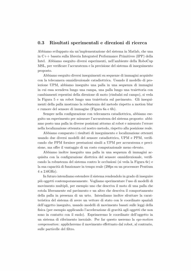
In this work we deal with balls and robots as objects to track, so weshould use a polygonal model of a sphere (see Figure 4.2) and a polygonalmodel of a cylinder as object 3D models. Given the simple nature of the3D shapes and taking advantage of their rotational symmetry, we are ableto select a set of contour point directly in 3D, and then project them toform a sampled representation of the 2D hypothetical contour. For a ballat a certain relative position, the 3D contour points lie on the intersectionbetween its spherical surface and the plane orthogonal to the line connectingthe virtual projection center to the center of the sphere, see Figure 4.3. Weobtain the set of 3D contour points by rotating and shifting (in accordto the position of the ball) a set of initial 3D points, equally distributedalong a circle with the same radius as that of the ball. The same method,with a different initial distribution of the points, is used for the robot, seeFigure 4.4.
The objective for the use of the 3D model is to define two sets of pixelsfor every hypothesis, one characterizing the color on the inner boundary ofthe projected contour and the other characterizing the color on the outer
22 Chapter 4. Model-based detection in omnidirectional images
Figure 4.2: Polygonal model of a sphere (some of the faces have been removed for
visualization).
Figure 4.3: Plot of the 3D points projected to obtain the 2D contour points for balls at
different positions. The black line connects the projection center to the ground plane.
Figure 4.4: Plot of the 3D points projected to obtain the 2D contour points for robots
at different positions. Again, the black line connects the projection center to the ground
plane.

4.2. 3D model 23
boundary. For this purpose, we use one of two methods: one based on simplesampling and the other one based on B-splines.
4.2.1 Selection of boundary pixels using sampling
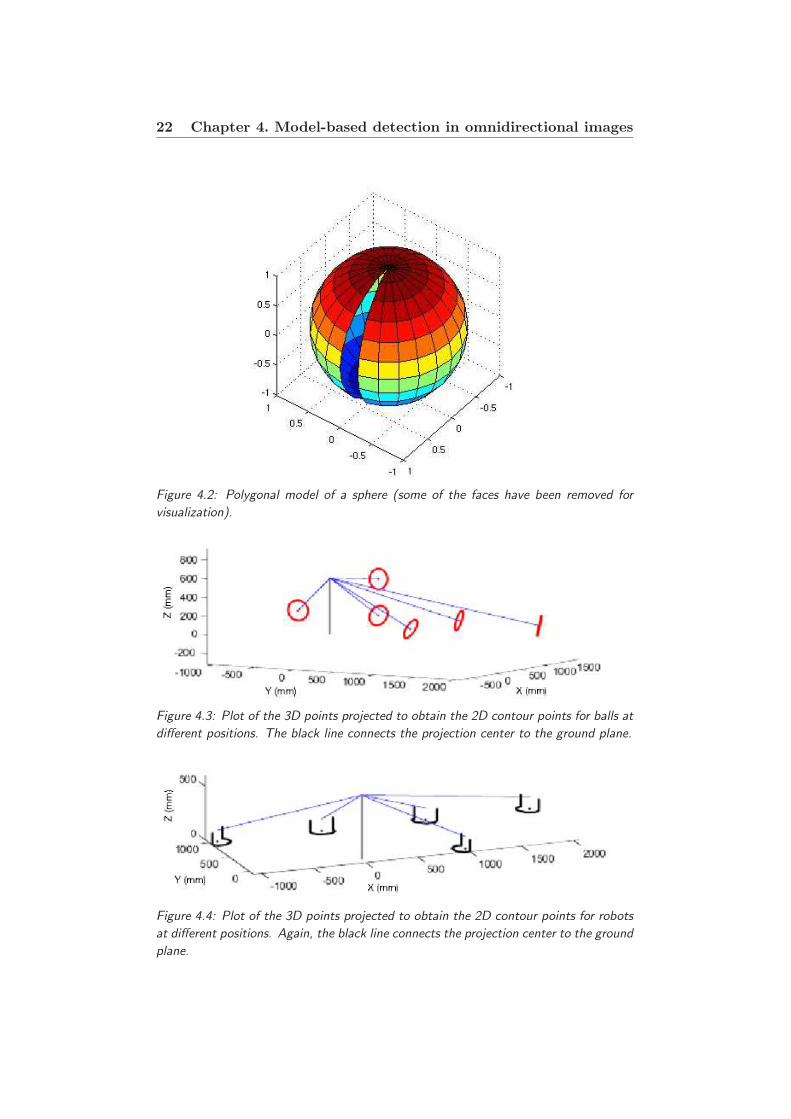
In this method we define the inner and outer boundary pixel sets by project-ing two different 3D contours, one larger than the actual size of the trackedobject, for the outside pixels, and one smaller than that for the inside pix-els, see Figure 4.5a. Varying the size difference between tracked object andinner and outer 3D contours enables the user of the tracking system to setthe balance between precision and processing time: the smaller the size dif-ference, the higher the precision of the estimate, but the higher the numberof particles needed and so the computation time. In our experiments oftracking the ball, which has a radius of 110mm, the 3D points were placedalong circumferences of 99mm and 121mm respectively (a 10% differencefrom the actual value). This method is fast and has the advantage of beingbased on 3D distances, rather than on image distances. This means thatthe distance between projected inner and outer contour adapts to the sizeof the projected object, but stays the same in real world coordinates, seeFigure 4.5b and 4.5c.
This method has one important drawback: whenever the shape projectedby an object becomes too small, the inner and outer contours of an objectsuperimpose and the tracking method fails. One solution to this would beto check the degree of superimposion after the projection of an hypothesis’contours. A good measure for this would be the relative number of innerboundary pixels which are also outer boundary pixels. When the super-imposion would exceed a given threshold, new inner and outer pixels setsshould be built, for example selecting pixels standing along normals to thehypothesized object contour, at a two pixels distance from it.
One interesting characteristic of this approach is that the number ofpoints used to build the color histograms can be varied: increasing suchnumber enhances the robustness of the tracker, while decreasing it makes thetracker faster, diminishing the number of projections to be made, togetherwith the operations performed to build each color histogram.
4.2.2 Selection of boundary pixels using B-splines
In this method we project the sample-based hypothetical contour of an hy-pothesis onto the image plane, model it with a B-spline and select inner andouter boundary pixels along normals to the spline.
24 Chapter 4. Model-based detection in omnidirectional images
(a)
(b) (c)
Figure 4.5: (a) 3D points modeling the hypothetical ball contour (red) and 3D points
used to select inner and outer boundary pixel sets (black). (b) and (c) Examples of the
pixel selection resulting from projecting the 3D model onto an image (after rotation
and translation). White pixels represent the projected contour, black pixels are the ones
selected to represent the color in the contour inner and outer boundaries.

4.2. 3D model 25
A B-spline has the following representation:
f(t) =k−m−1∑
i=0
ciBmi (t), t ∈ [tm, tk−m] (4.1)
where {Bmk (t), k = 0, . . . , k−m−1} is the set of basis functions such that
Bmi (t) ≥ 0, and
∑i Bm
i (t) = 1; {c0, c1, . . . , ck−m−1} is the set of coefficientsand [ti−1, ti] is an interval in which the spline functions are polynomial andexhibit a certain degree of continuity at the knots.
Planar curves are simply the R2 version of Equation 4.1:
v(t) ≡ [x(t) y(t)] =k−m−1∑
i=0
ciBmi (t) (4.2)
A discretized spline is a set of N equispaced samples of v(t) collected as theN × 2 vector:
v = [vT0 , . . . ,v
TN−1] = [x y], N > k (4.3)
If we arrange the coordinates of control points into a parameter θ(k):
θ(k) = [cT0 , . . . , cTk−1]
T = [θx(k) θy
(k)]1, (4.4)
the discretized closed spline v can be obtained by the matrix product
v = B(k)θ(k) ⇔ {x = B(k)θx(k); y = B(k)θ
y(k)}, (4.5)
where the elements of B(k) are [B(k)]ij = Bj(t0 + (tk−t0)iN ).
In computer graphics m = 3 or 4 is generally found to be sufficient.Herein, we use quadratic B-splines, i.e., m = 3.
After obtaining the 2D points {dnboundary}, n = 1, . . . , N , we convert
them into a B-spline which best fits to this set. Assuming that we knownthe knots, the N × k matrix B(k) can be computed. Thus, given the vectord with N data points and a choice of k, a N × k matrix B(k) can be builtand its pseudo-inverse B†
(k) computed. The estimated control points are
given by θ(k) = B†(k)d, with B†
(k) = (BT(k)B(k))−1BT
(k) and the curve is given
by v = [B†(k)x B†
(k)y] = B(k)θ(k). The regions in which the histogram iscomputed are defined at the points of the normal lines radiating from thediscrete B-spline curve v, i.e.
H =N⋃
i=1
(±∆)v(si) n(si) (4.6)
1(k) is the total of number of control points

26 Chapter 4. Model-based detection in omnidirectional images
(a) (b)
Figure 4.6: Generic B-spline shape with the orthogonal lines. Control points are repre-
sented by circles (a). Bold lines show the image locations where the histogram values
are collected (b).
where the sign +, and − distinguishes whether the inspection is performedinside (Hinner) or outside (Houter) the reference contour respectively; n(si)is the normal vector at the point si; ∆ ∈ [0, 1], Figure 4.6 depicts thetechnique proposed herein. A quadratic B-spline of a generic shape and theorthogonal lines are shown in Figure 4.6a. Figure 4.6b displays the lines atwhich the histogram values are collected. The pixels selected to evaluate onehypothesis (one hypothesis shown for each image) are depicted in Figure 4.7.In some cases, i.e., when using cameras displaying color mosaicking errorsat image edges, it may be convenient to avoid sampling at the middle of theline segment. In our case, however, color information at the contour pixelsis quite acceptable and one can perform the inspection along the entire linesegment.
4.3 Color model
We use color histograms to model the color of the object to track and tocharacterize the color of the two image regions surrounding an hypotheticalcontour.
We use the HSI (Hue, Saturation, Intensity) color space in the Matlabimplementation of the tracker. We choose the HSI color space because theHue component separates well colors of pixels belonging to the ball fromcolors of pixels belonging to the rest of the RoboCup environment, see Fig-ure 4.8. We calculate the H and S values of each pixel as for the HSV colorspace, but prefer Intensity, I=(R+G+B)/3 to Value, V=max(R,G,B), asIntensity exploits all the available RGB information, while V discards thevalues of the two non-maximum RGB channels. We set the number of bins

4.3. Color model 27
Figure 4.7: Close-up showing the pixels used to evaluate one hypothesis (one for each
image), selected using B-splines. Yellow and blue pixels are used to build the inner and
outer color histogram, respectively.

28 Chapter 4. Model-based detection in omnidirectional images
for the HSI histogram to Bh = 12, Bs = 12, Bi = 4. We set the number ofbins for the Intensity channel to a smaller value than the other two in orderto achieve some robustness w.r.t. illumination intensity changes. Ignoringthe Intensity channel altogether would have prevented us from distinguishingwhite and black object from the others.
We use the YUV color space in the C++ real-time implementation ofthe tracker because that is the color space in which the camera provides theimages. This choice allows us to save processing time, as we do not performa color-space transformation, and maintains the desirable characteristic ofa color representation in which the brightness channel (Y) is orthogonal tothe others. We set the number of bins for the YUV histogram to By = 4,Bu = 8, Bv = 8. We set the number of bins for the V channel to a smallervalue than the other two, in order to achieve robustness w.r.t. illuminationchanges, as in the previous case.
A color histogram is a non parametric statistical description of a colordistribution, in terms of occurrences of different color classes. Let us denote
bt(d) ∈ {1, . . . , B}, (4.7)
the bin index associated with the color vector at pixel location d and framet. Then the histogram of the color distribution of a generic set of points canbe computed by a kernel density estimate
H .= {h(b)}b=1,...,B (4.8)
of the color distribution at frame t, where each histogram bin is given asin [10]
h(b) = β∑
n
δ[bt(dn)− b] (4.9)
where δ is the Kronecker delta function, β is a normalization constant whichensures h to be a probability distribution
∑Bb=1 h(b) = 1. We encode each
color histogram as a 12× 12× 4 or a 4× 8× 8 matrix in the HSI and YUVcase respectively.
The color model for each object was built collecting a set of images inwhich the object is present, and calculating the color histogram on the (handlabeled) pixels belonging to the specific object. All object pixels were usedto train the color histograms, whereas in run-time, only a subset of pointsis used.

4.3. Color model 29
(a)
(b)
(c)
Figure 4.8: (a) Projection in the HSB(=HSV) space of pixels belonging to the ball,
taken from different images. (b) Projection in the HSB space of pixels belonging to
an image depicting a typical RoboCup environment. (c) Setting two thresholds on the
Hue would provide a reasonable separation between the two classes.
30 Chapter 4. Model-based detection in omnidirectional images
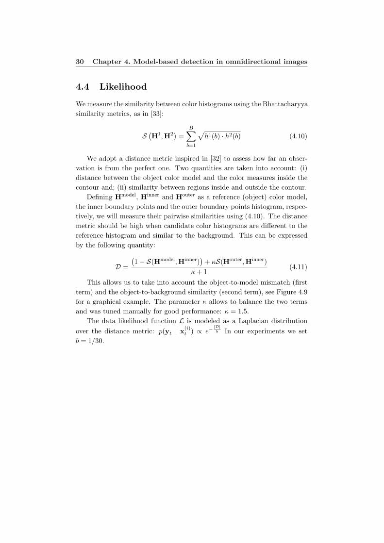
4.4 Likelihood
We measure the similarity between color histograms using the Bhattacharyyasimilarity metrics, as in [33]:
S (H1,H2
)=
B∑
b=1
√h1(b) · h2(b) (4.10)
We adopt a distance metric inspired in [32] to assess how far an obser-vation is from the perfect one. Two quantities are taken into account: (i)distance between the object color model and the color measures inside thecontour and; (ii) similarity between regions inside and outside the contour.
Defining Hmodel, Hinner and Houter as a reference (object) color model,the inner boundary points and the outer boundary points histogram, respec-tively, we will measure their pairwise similarities using (4.10). The distancemetric should be high when candidate color histograms are different to thereference histogram and similar to the background. This can be expressedby the following quantity:
D =
(1− S(Hmodel,Hinner)
)+ κS(Houter,Hinner)
κ+ 1(4.11)
This allows us to take into account the object-to-model mismatch (firstterm) and the object-to-background similarity (second term), see Figure 4.9for a graphical example. The parameter κ allows to balance the two termsand was tuned manually for good performance: κ = 1.5.
The data likelihood function L is modeled as a Laplacian distributionover the distance metric: p(yt | x(i)
t ) ∝ e−|D|b In our experiments we set
b = 1/30.

4.4. Likelihood 31
Figure 4.9: Three hypothetical contours projected on one image. Contour A has a
low likelihood, because of high object-to-model mismatch (the inner boundary of the
contour is not orange) and high object-to-background similarity (the colors of inner
and outer boundary of the contour are pretty similar). Contour C is associated with
a medium likelihood, because of low object-to-model mismatch (the inner boundary
of the contour is orange), but high object-to-background similarity (also the outer
boundary of the contour is quite orange). Contour B has a high likelihood because of
low object-to-model mismatch and low object-to-background similarity.

32 Chapter 4. Model-based detection in omnidirectional images

Chapter 5
Tracking with particle filters
“If I could remember the names of all these particles, I’d be a botanist.1.”
Enrico Fermi
In this chapter we describe the methods employed for 3D target trackingwith particle filters.
5.1 Particle filter tracking.
We are interested in computing, at each time t ∈ N, an estimate of the 3Dpose of a target. We represent this information as a “state-vector” defined bya random variable xt ∈ Rnx whose distribution in unknown (non-Gaussian);nx is the dimension of the state vector. In the present work we are mostlyinterested in tracking balls and cylindrical robots, whose orientation is notimportant for tracking. However, the formulation is general and can easilyincorporate other dimensions in the state-vector, e.g., target orientation andspin.
Let xt = [x, y, z, x, y, z]T , with (x,y,z), (x,y,z) the 3D cartesian positionand linear velocities in a robot centered coordinate system. The state se-quence {xt; t ∈ N} represents the state evolution along time and is assumedto be a Markov process with some initial distribution p(x0) and a transitiondistribution p(xt | xt−1).
The observations taken from the images are represented by the randomvariable {yt; t ∈ N}, yt ∈ Rny , and are assumed to be conditionally inde-pendent given the process {xt; t ∈ N} with marginal distribution p(yt | xt),where ny is the dimension of the observation vector.
1In this occasion Fermi was referring to subatomic particles, but he is often credited
with the development of the Monte Carlo method.

34 Chapter 5. Tracking with particle filters
In a statistical setting, the problem is posed as the estimation of theposteriori distribution of the state given all observations p(xt | y1:t). Underthe Markov assumption, we have:
p(xt | y1:t) ∝ p(yt | xt)∫p(xt | xt−1) p(xt−1 | y1:t−1)dxt−1 (5.1)
The previous expression tells us that the posteriori distribution can be com-puted recursively, using the previous estimate, p(xt−1 | y1:t−1), the motion-model, p(xt | xt−1) and the observation model, p(yt | xt).
To address this problem we use particle filtering methods. Particle filter-ing is a Bayesian method in which the probability distribution of an unknownstate is represented by a set of M weighted particles {x(i)
t , w(i)t }M
i=1 [13]:
p(xt | y1:t) ≈M∑
i=1
w(i)t δ(xt − x(i)
t ) (5.2)
where δ(·) is the dirac delta function. Based on the discrete approximationof p(xt | y1:t), different estimates of the best state at time t are possible tobe devised. For instance we may use the Monte Carlo approximation of theexpectation:
x .=1M
M∑
i=1
w(i)t x(i)
t ≈ E(xt | y1:t), (5.3)
or the maximum likelihood estimate:
xML.= argmaxxt
M∑
i=1
w(i)t δ(xt − x(i)
t ) (5.4)
To compute the approximation to the posteriori distribution, a typicaltracking algorithm works cyclically in three stages:
1. Prediction - computes an approximation of p(xt | y1:t−1) , by movingeach particle according to the motion model;
2. Update - each particle’s weight i is updated using its likelihood p(yt |x(i)
t ):w
(i)t ∝ w
(i)t−1p(yt | x(i)
t ) (5.5)
3. Resampling - the particles with a high weight are replicated and theones with a low weight are forgotten.
For this purpose, we need to model probabilistically both the motiondynamics, p(xt | xt−1) , and the computation of each particle’s likelihoodp(yt | x(i)
t ).

5.2. Initialization of the particle filter 35
5.1.1 Motion model
In the system proposed herein we assume motion dynamics follow a standardautoregressive dynamic model:
xt = Axt−1 + wt, (5.6)
where wt ∼ N (0, Q). The matrices A, Q, could be learned from a set ofrepresentative correct tracks, obtained previously (e.g., see [5]), however, wechoose pre-defined values for these two matrices. Since the coordinates inthe model are real-world coordinates, the motion model for a tracked objectcan be chosen in a principled way, both by using realistic models (constantvelocity, constant acceleration, etc.) and by defining the covariance of thenoise terms in intuitive metric units.
We use a constant velocity model, in which the motion equations corre-spond to a uniform acceleration during one sample time:
xt = Axt−1 +Bat−1, A =
[I (∆t)I0 I
], B =
[(∆t2
2 )I(∆t)I
](5.7)
where I is the 3 × 3 identity matrix and at is a 3 × 1 white zero meanrandom vector corresponding to an acceleration disturbance. We have set∆t = 1 for all the experiments, whereas the covariance matrix of the randomacceleration vector was fixed at:
cov(at) = σ2I, σ = 90mm/frame2 (5.8)
5.1.2 Observation model
The observation model allows us to compute the likelihood that a partic-ular hypothesis (state vector) generated the observation (image) we have.We compute the likelihood of an object state, given the object model, theprojection model for the omnidirectional camera and one omnidirectionalimage, as described in Chapter 4.
5.2 Initialization of the particle filter
The PF needs an initial distribution of particles to start from. In the caseof the dioptric camera and the ball, we use a method designed to workcoupled with a detection module (possibly based on color segmentation): itreceives as input an image and a pair of image coordinates, identifying thecenter of the projected ball. These coordinates are now provided by a user,

36 Chapter 5. Tracking with particle filters
Figure 5.1: Initialization of the filter: particles are spread along a 3D ray based on a
couple of image coordinates selected by a detection algorithm. The distribution used
to initialize the filter will be Gaussian, centered on the particle, among the ones spread
along the ray, with the highest likelihood.
which has to choose a pixel near the center of the projected ball, but shouldin the future be provided by a detection module. We apply the inverseequidistance projection to the coordinates and thus select the direction ofthe corresponding 3D ray joining the projection center to the ground plane(see Figure 5.1). We spread some particles along this ray and calculatethe likelihood for every particle, based on the information contained in theimage.
The distribution of particles for the PF is then initialized by a Gaussiandistribution, centered at the position of the maximum likelihood particle.The velocities are also initialized by a Gaussian distribution, with mean 0.
In the other cases we initialize the particles by a Gaussian distributionwith large variance, centered at rough estimates of the object’s initial po-sition and velocity. This method is not automatic, so it can not be usedin an autonomous robot, unless in very specific cases. One such case is forexample when robots communicate among them, so one robot can detectthe ball and pass its estimates on position and speed to the others. Whenwe track robots, both position and velocity are only bidimensional, as MSLrobots do not jump yet.

Chapter 6
Experimental results
“No amount of experimentation can ever prove me right;
a single experiment can prove me wrong.”
Albert Einstein
We ran several experiments to assess the accuracy and precision of theproposed tracking method: in the catadioptric setup, using UPM to modelthe camera projection, we tracked a ball rolling down a ramp, a ball bouncingon the floor and a robot maneuvering. We furthermore ran an experimentplacing a still ball at different positions around the robot and measuring theerror of the detected position with respect to the ground truth.
We compared the results obtained in the tracking and detection, usingUPM and PPM to model the catadioptric sensor.
Eventually, we tracked a ball in the dioptric setup, testing the systemfor robustness against occlusions. We also assessed the time needed by theC++ implementation of our tracker to elaborate one image, verifying it canrun in real-time.
6.1 Catadioptric setup, UPM
In the first experiment we tested the proposed method on sequences of im-ages acquired with our catadioptric omnidirectional camera, which we modelwith the UPM. We used the Matlab implementation of the code, setting thenumber of particles to 10000. This value was intentionally very high, as weintended to test the precision of the tracker in an off-line setting. To samplethe pixels in order to build the inner and outer color histograms for eachhypothesis we projected a sphere with respectively 0.9 and 1.1 the radius of

38 Chapter 6. Experimental results
the actual ball. For each projection we used 50 points, uniformly distributedon each 3D contour.
The initial position for the particles was obtained sampling a 3D Normaldistribution, the mean and standard deviation of which were manually set.The initial velocity was also manually set, equal for every particle. Theparameter k was set to 1.5, meaning that we wanted the difference betweeninner color and outer color to be more discriminative than the similaritybetween inner color and model color. We repeated the tracking 10 times onevery image sequence, to evaluate the precision of the tracker.
6.1.1 Ball tracking
In the first part of this experiment, we tracked a ball rolling down a two-railramp. The projection of the ball on the image plane changes dramatically insize after some frames (see Figure 6.1), due to the nature of the catadioptricsystem used. The images are affected by both motion blur and heavy sensornoise (see Figure 6.2). This image sequence was acquired with a frame rateof 20fps. The results of the tracking are visible in Figure 6.3a.
In the second part of this experiment we tracked a ball bouncing onthe floor. The frame rate in this case was of 25fps. The image sequencebegins with the ball about to hit an obstacle on the ground, while movinghorizontally. The collision triggers a series of parabolic movements for theball, which is tracked until it hits the ground for the fourth time. The resultsare visible in Figure 6.3b.
6.1.2 Robot tracking
In this experiment we tracked a robot moving along a straight line, turningby 90 degrees and continuing its motion along the new direction (Figure 6.4).The vertical position and speed of the tracked object were constrained tobe null. The injected velocity noise was, thereafter, distributed as a 2DNormal. To sample the pixels in order to build the inner and outer colorhistogram for each hypothesis we projected the contour of an 8-sided-prismwith respectively 0.75 and 1.25 the size of the actual robot. The size dif-ference between the projected models and the actual one is greater than inthe case of the ball due to the fact that the model for the robot does notexactly fit its actual shape. For each projection, 120 points were used. Werepeated the tracking 10 times and results are shown in Figure 6.5.

6.1. Catadioptric setup, UPM 39
(a) (b)
Figure 6.1: Ball rolling down a ramp. Frames 1, 11 and 21 of the sequence (a) and
three corresponding close-ups of the tracked ball with the contour of the best hypothesis
drawn in white (b). The pixels marked in black are the ones used to build the color
histograms.

40 Chapter 6. Experimental results
Figure 6.2: Close-ups of the ball showing motion blur and sensor noise.
6.1.3 Error evaluation
In this experiment we placed a ball at various positions around a robotand confronted the positions measured with our system against the groundtruth. The positions were either in front of the robot, on its right, on itsleft or behind it, and either on the floor or at a height of 340mm.
As we were interested in studying the localization error “at convergence”,we run the particle filter three times on each image. In the first step, theparticle filter was initialized with the ground truth position of the ball andthe particles were generated with a 3D Normal p.d.f. with that position asmean and a standard deviation of 100mm. In the second step the particleswere generated around the position estimated in step one, with a standarddeviation of 70mm. In the third step the particles were generated aroundthe position estimated in step two, with a standard deviation of 40mm.
Both the ground truth and the estimated ball positions are shown inFigure 6.6. It is noticeable some bias mainly in the vertical direction, due tomiscalibration of the experimental setup. However, we are mostly interestedin evaluating errors arising in the measurement process. Distance to thecamera is an important parameter in this case, because target size variessignificantly. Therefore, we have performed a more thorough error analysisevaluating its characteristics as a function of distance to the camera.
In Figure 6.7, we plot the measured error in spherical coordinates (γ–distance, φ–elevation, ψ–azimuth), as a function of distance to camera’svirtual projection center. The first plot shows that radial error character-istics are mostly constant along distance, with a systematic error (bias) ofabout 46mm, and standard deviation of about 52mm. This last value is the

6.1. Catadioptric setup, UPM 41
(a)
(b)
Figure 6.3: (a) Ball rolling down the ramp: plot of the tracked paths resulting from 10
runs of the algorithm performed on the same image sequence. The 10 blue lines with
red points represents the 10 3D estimated trajectories of the ball, the blue lines are the
projection of these trajectories on the ground and lateral plane. (b) Ball jumping: same
kind of plot for the estimated trajectories of the ball in the jump image sequence.
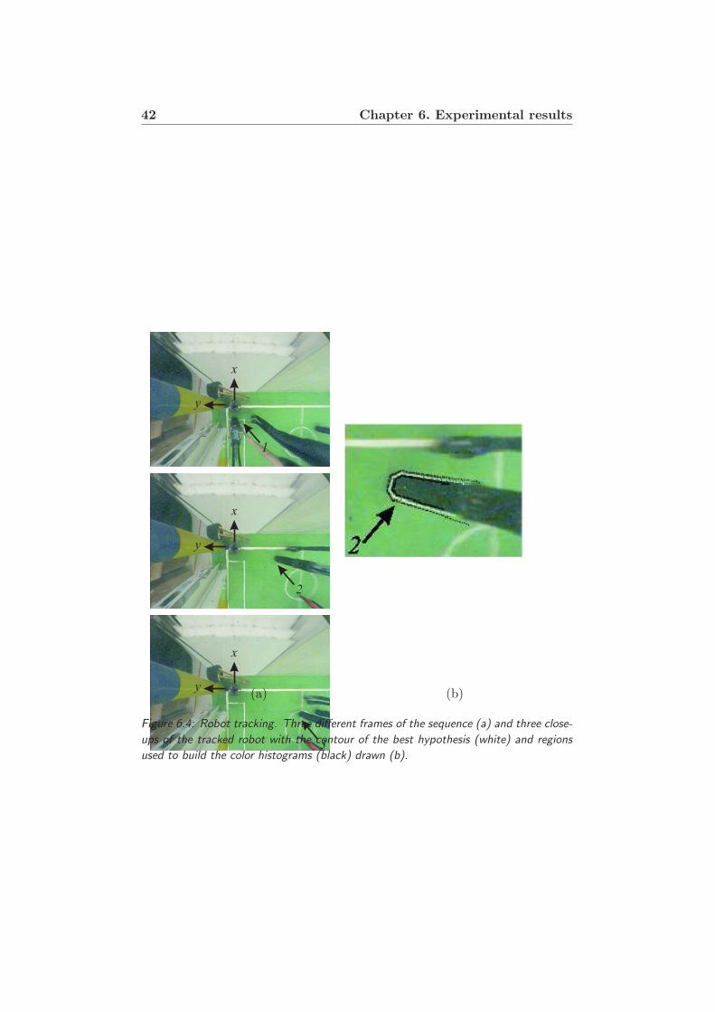
42 Chapter 6. Experimental results
(a) (b)
Figure 6.4: Robot tracking. Three different frames of the sequence (a) and three close-
ups of the tracked robot with the contour of the best hypothesis (white) and regions
used to build the color histograms (black) drawn (b).

6.2. Catadioptric setup, UPM and PPM experimentalcomparison 43
Figure 6.5: Reconstructed robot trajectory - a view from the top of 10 estimated
trajectories.
one we should retain for characterizing the precision of the measurementprocess. The second plot shows the elevation error, where it is evident adistance dependent systematic error. This has its source on a bad approx-imation of the projection model for distances close to the camera. Finally,the third plot shows the azimuthal error. It can be observed that there isa larger random error component at distances close to the camera, but thisjust a consequence of the fact that equal position errors at closer distancesproduce larger angular errors.
6.2 Catadioptric setup, UPM and PPM experi-
mental comparison
In this experiment we compared the results obtained modeling the catadiop-tric omnidirectional camera with either UPM and PPM.
6.2.1 Error evaluation
We repeated the experiment described in Section 6.1.3, using either PPMand UPM to model the camera. Both models were calibrated with thesame 3D- and imaged-points data. The color histograms in this experimentwere computed based on the pixels sampled with the B-spline method, asdescribed in Section 4.2.2.
We have computed the errors between ground truth and measurements,in spherical coordinates γ, φ and ψ, respectively distance, elevation andazimuth. Results for the errors’ mean and standard deviation are presented

44 Chapter 6. Experimental results
−4000 −3000 −2000 −1000 0 1000 2000 3000 4000 5000
−4000
−3000
−2000
−1000
0
1000
2000
3000
X (mm)
Y (
mm
) (a)
(b)
Figure 6.6: Two views of ground truth (blue) and measurements (red).
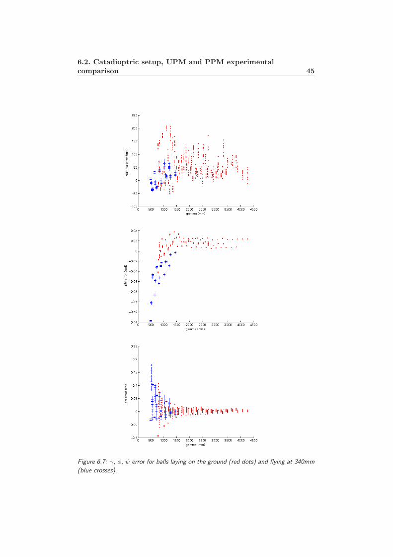
6.2. Catadioptric setup, UPM and PPM experimentalcomparison 45
Figure 6.7: γ, φ, ψ error for balls laying on the ground (red dots) and flying at 340mm
(blue crosses).

46 Chapter 6. Experimental results
UPM PPMmean γ error (mm) -19.8712 -18.2616std.dev γ error (mm) 48.1137 47.9484mean φ error (rad) 0.0005 0.0006std.dev φ error (rad) 0.0310 0.0276mean ψ error (rad) 0.0072 0.0072std.dev ψ error (rad) 0.0314 0.0312Computation Time (ms) 11.2 6.3
Table 6.1: Comparison of errors measured with the UPM vs PPM. Last line shows the
computation times for projecting 50000 points, on a P4 2.6GHz computer.
Figure 6.8: Ball jumping: plot of the tracked paths resulting from 10 runs of the
algorithm performed on the same image sequence. The estimated trajectories using the
PPM and the UPM models are shown, respectively, with blue and red lines. Both the
3D trajectory and its projections on the ground and lateral planes are shown.
in Table 6.1. As can be observed from the table, there are no significantdifferences between the two projection models. However, the computationtime for PPM is about half the time taken by the UPM (last line of Table6.1). Therefore, the usage of the PPM is advantageous for the overall 3Dtracking system, since it reduces computation time for the same level ofprecision.
6.2.2 Ball tracking
In this experiment we repeated the tracking on the sequence of the jumpingball (see Section 6.1.1), using PPM instead of UPM. A comparison of theresults obtained using the two models is shown in Figure 6.8. No noticeabledifferences are observed between the two models, but computational savingsjustify the choice of the PPM model.

6.3. Dioptric setup 47
6.3 Dioptric setup
In this set of experiments we tested the proposed method on sequences ofimages acquired with our dioptric omnidirectional camera, which we modelwith the EPM. We used the C++ implementation of the tracker, the oneexploiting the vector and matrix operations provided by the IPP library, byIntel. To sample the pixels in order to build the inner and outer color his-tograms for each hypothesis we projected a sphere with respectively 0.7 and1.3 the radius of the actual ball. This provided us with a “wider” and “flat-ter” likelihood function than in experiment described in Section 6.1.3.Thischoice allowed us to use few particles, namely 300, trading some precision forspeed. For each projected contour we used 50 points, uniformly distributedon each 3D contour. With these settings, the tracker run at more than 29fpson a 2.6GHz Pentium 4 processor. The color model, a YUV histogram, wasobtained from manually selected regions, belonging to an image sequencewhich was not used for tracking (see Figure 6.9). The image sequences forthe various experiments were acquired at different frame rates, with differ-ent camera settings and different illumination conditions. The tracker wassuccessful in all its runs, in spite of these difficulties, which made the colorof the ball look different in every sequence (see Figure 6.10). The trackeralso successfully handled reflexions and shadows, which made the ball looknonhomogeneous in color.
The initial distribution of the particles was set up in two steps: a de-tection step and a real initialization step. In the first step, particles werespread along the 3D ray corresponding to a couple of user-selected imagecoordinates. A 3D point was chosen in correspondence of the particle withthe highest likelihood. In the second step, the set of particles was initializedby a Gaussian distribution with large variance, centered at the selected 3Dpoint. The parameter k was, as in the other experiments, set to 1.5. Werepeated the tracking 10 times on each image sequence, in order to test theprecision of the tracking method.
6.3.1 Jumping ball
We tracked a ball jumping on the floor and bouncing off a wall (see Fig-ure 6.11). This experiment shows the ability of our tracker to work with off-the-floor targets. The trajectories resulting from the 10 runs of the trackershow that, in spite of using few particles, the estimation of the position ofthe ball is precise (Figure 6.12). This image sequence was acquired at 25fps.

48 Chapter 6. Experimental results
Figure 6.9: The color histogram for the experiments with the dioptric camera was built
based on the non-white pixels of this image.
6.3.2 Occlusions
We tracked a ball passing behind an obstacle (see Figure 6.13 and 6.14)and a ball which gets to be halfway hidden by a robot ( see Figure 6.15and 6.16). These experiments show the robustness of our tracking methodagainst occlusions. The method succeeds in tracking the ball in both cases,showing some inaccuracy when the ball is hidden by the robot.
6.3.3 Multiple objects
In this experiment we tracked a ball along a sequence in which its projectiononto the image overlaps with that of another ball. Our tracker is not amultiple object tracker, but we show that its behavior in such a case is stillsensible: it either keeps tracking the ball it was initialized on or switches tothe other. The results of the tracking are visible in Figure 6.17 and 6.18.

6.3. Dioptric setup 49
Figure 6.10: Close-ups on the ball in images from the various experiments. Note the
difference in the color of the ball and the reflexions which make pixels belonging to the
projection of the ball look yellow, rather than orange.

50 Chapter 6. Experimental results
(a) (d)
(b) (e)
(c) (f)
Figure 6.11: Ball jumping. Six frames from the tracked sequence.

6.3. Dioptric setup 51
Figure 6.12: Ball jumping: plot of the tracked paths resulting from 10 runs of the
algorithm performed on the same image sequence. The pyramid represents the robot
acquiring the image sequence. The tracked paths start in 1. At first, the ball is held
by a person who lowers it (tracks from area 1 to 2), then the ball is thrown in the air,
bounces on the floor and then bounces on the floor and off the wall at the same time
(3). The tracked paths end in 4.

52 Chapter 6. Experimental results
(a)
(b)
(c)
Figure 6.13: Three frames of the tracked sequence when the ball is occluded by the
bar which sustains the camera.

6.3. Dioptric setup 53
(a)
(b)
Figure 6.14: Top view (a) and 3D plot (b) of the 10 tracked trajectories. The pyramid
represents the robot acquiring the image sequence. 1 denotes the beginning of the
trajectories, 2 denotes the area when the ball is occluded by the bar and moving slowly,
a small error in the trajectories can be noticed (in the trajectories there are two abrupt
changes of direction, in correspondence with the beginning and end of the occlusion).
3 denotes another passing of the ball behind the obstacle, while 4 denotes the end of
the trajectories.

54 Chapter 6. Experimental results
(a) (c)
(b) (d)
Figure 6.15: Two frames of the tracked sequence in which the ball is occluded by
another robot. In the first row the ball is still fully visible, while in the second it is
halfway hidden by the robot. In the first column the original images are shown, in
the second one the inner and outer contours of the maximum likelihood hypothesis are
drawn in white, while those of the hypothetical position corresponding to mean of all
the particles, weighted by their likelihood, are drawn in black.

6.3. Dioptric setup 55
Figure 6.16: Plots of the 10 tracked trajectories of the ball. The tracked paths begin
in 1. When the ball is fully visible (from area 1 to 2 and from 4 to 5) the precision of
the tracker is lower than in the previous experiment. This depends on the fact that in
this experience the ball is farther from the robot acquiring the image sequence. Farther
objects can be localized with less precision because of the projection performed by the
dioptric omnidirectional camera. When the ball is hidden (from area 2 to 4), the esti-
mate of the position becomes less accurate, as the tracker associates higher likelihoods
to smaller contours, corresponding to balls which are farther from the observing robot.

56 Chapter 6. Experimental results
(a) (d)
(b) (e)
(c) (f)
Figure 6.17: Image frames from the sequence with two overlapping balls.

6.3. Dioptric setup 57
Figure 6.18: Tracked trajectories for the sequence with overlapping balls. The tracked
paths start in area 1. Some inaccuracy in the localization of the tracked object can
be seen in correspondence of the overlapping (2). In nine cases out of ten, the tracker
followed the ball it was initialized on (ending in area 3), while in one case it switched
to tracking the other ball (ending in area 3’).

58 Chapter 6. Experimental results

Chapter 7
Conclusions and future work
“The end is the beginning
of the end.”
Billy Corgan, The Smashing Pumpkins.
In this thesis we presented a model-based 3D tracker for autonomousrobots equipped with omnidirectional cameras. The tracker was designedto work in the structured, color-coded environment of the RoboCup MSL.The system was based on a particle filter, for robustness against occlusionsand ambiguity. The chosen object model comprises a 3D shape model, acolor model and a motion model. The observation model was designed tobe robust against motion blur, image sensor noise and illumination changes.The system works with either a catadioptric or a dioptric omnidirectionalcamera.
We developed both a Matlab and a C++ implementation of the tracker.We ran several experiments, in a RoboCup MSL scenario, to assess the
accuracy and precision of the proposed tracking method with color-codedobjects.
In the catadioptric setup, using UPM to model the camera projection,we tracked a ball rolling down a ramp, a ball bouncing on the floor and arobot maneuvering. These experiments on ball tracking show the robustnessof the method with respect to motion blur and image sensor noise.
Still in the catadioptric setup, we ran an experiment to assess the ac-curacy of the system, placing a still ball at different positions around therobot and measuring the error of the detected position with respect to theground truth.
We compared the results obtained in tracking and detection, using UPMand PPM to model the catadioptric sensor, verifying that PPM provides the

60 Chapter 7. Conclusions and future work
same level of precision and accuracy of UPM, but at a smaller computationalcost.
Eventually, we tracked a ball in the dioptric setup, testing the system forrobustness against occlusions and real-time capabilities, verifying that theC++ implementation, exploiting the vector and matrix operations providedby the IPP library, can run at 29fps on a P4 2.6GHz processor.
In future work we intend to extend the system with the ability to trackmultiple objects. We will introduce the use of multiple motion models, forexample use a model describing the motion of a ball rolling freely and an-other describing the motion of a ball bouncing against an obstacle. We alsointend to use physics-based motion models (e.g. applying gravitational ac-celeration to particles which model flying balls). We will express the target’scoordinates in an inertial reference frame, instread of the robot-centered onewe use now. This will be combined with ego-motion compensation: applyingthe inverse motion of the robot to the filter’s particles. We also plan to testthe tracker in a non-color-coded environment.

Bibliography
[1] George A. Bekey. Autonomous Robots. MIT, 2005.
[2] R. Benosman and S.B. Kang, editors. Panoramic Vision. SpringerVerlag, 2001.
[3] ST Birchfield and S. Rangarajan. Spatiograms versus Histograms forRegion-Based Tracking. Computer Vision and Pattern Recognition,2005. CVPR 2005. IEEE Computer Society Conference on, 2, 2005.
[4] G.R. Bradski et al. Computer vision face tracking for use in a perceptualuser interface. Intel Technology Journal, 2(2):12–21, 1998.
[5] Gilles Celeux, J. Nascimento, and J. S. Marques. Learning switchingdynamic models for objects tracking. Pattern Recognition, 37(9):1841–1853, 2004.
[6] P. Chang and J. Krumm. Object recognition with color cooccurrencehistograms. Proceedings of the IEEE Computer Society Conference onComputer Vision and Pattern Recognition, 2:498–504, 1999.
[7] Y. Cheng. Mean shift, mode seeking, and clustering. IEEE Transactionson Pattern Analysis and Machine Intelligence, 17(8):790–799, 1995.
[8] C. Christoudias, B. Georgescu, and P. Meer. Synergism in low levelvision. International Conference on Pattern Recognition, 4:150–155,2002.
[9] RT Collins, Y. Liu, and M. Leordeanu. Online selection of discrimi-native tracking features. Pattern Analysis and Machine Intelligence,IEEE Transactions on, 27(10):1631–1643, 2005.
[10] D. Comaniciu, V. Ramesh, and P. Meer. Real-time tracking of non-rigid objects using mean shift. IEEE Conf. on Computer Vision andPattern Recognition, pages 142–151, 2000.
61

62 BIBLIOGRAPHY
[11] D. Comaniciu, V. Ramesh, and P. Meer. Kernel-based object track-ing. Pattern Analysis and Machine Intelligence, IEEE Transactionson, 25(5):564–577, 2003.
[12] I.J. Cox, S.L. Hingorani, et al. An efficient implementation of Reid’smultiple hypothesis tracking algorithm and its evaluation for the pur-pose of visual tracking. IEEE Transactions on Pattern Analysis andMachine Intelligence, 18(2):138–150, 1996.
[13] A. Doucet, N. de Freitas, and N. Gordon. Sequential Monte CarloMethods In Practice. Springer Verlag, 2001.
[14] K. Fukunaga and L. Hostetler. The estimation of the gradient of adensity function, with applications in pattern recognition. InformationTheory, IEEE Transactions on, 21(1):32–40, 1975.
[15] J. Gaspar, C. Decco, Jun Okamoto Jr, and J. Santos-Victor. Constantresolution omnidirectional cameras. 3rd International IEEE Workshopon Omni-directional Vision at ECCV, pages 27–34, 2002.
[16] J. Gaspar, N. Winters, and J. Santos-Victor. Vision-based naviga-tion and environmental representations with an omnidirectional cam-era. IEEE Transactions on Robotics and Automation, 16(6), 2000.
[17] T. Gevers and H. Stokman. Robust histogram construction from colorinvariants for object recognition. Pattern Analysis and Machine Intel-ligence, IEEE Transactions on, 26(1):113–118, 2004.
[18] C. Geyer and K. Daniilidis. A unifying theory for central panoramicsystems and practical applications. Conf. on Computer Vision andPattern Recognition, pages 445–461, 2000.
[19] Christopher Geyer, Tomas Pajdla, and Kostas Daniilidis. Short courseon omnidirectional vision. ICCV, 2003.
[20] R. Hicks and R. Bajcsy. Catadioptric sensors that approximate wide-angle perspective projections. Proceedings of the Computer Vision andPattern Recognition Conference, pages 545–551, 2000.
[21] C. Hue, J.P. Le Cadre, P. Perez, and R.I. IRISA. Tracking multipleobjects with particle filtering. Aerospace and Electronic Systems, IEEETransactions on, 38(3):791–812, 2002.

BIBLIOGRAPHY 63
[22] M. Isard and A. Blake. Contour Tracking by Stochastic Propagationof Conditional Density. Proceedings of the 4th European Conference onComputer Vision-Volume I-Volume I, pages 343–356, 1996.
[23] M. Isard and A. Blake. CONDENSATION: Conditional Density Prop-agation for Visual Tracking. International Journal of Computer Vision,29(1):5–28, 1998.
[24] M. Isard and J. MacCormick. BraMBLe: A Bayesian multiple-blobtracker. International Conference on Computer Vision, 2(5), 2001.
[25] R.E. Kalman. A new approach to linear filtering and prediction prob-lems. Journal of Basic Engineering, 82(1):35–45, 1960.
[26] J. Kannala and S. Brandt. A generic camera calibration method forfish-eye lenses. Pattern Recognition, 2004. ICPR 2004. Proceedings ofthe 17th International Conference on, 1, 2004.
[27] Z. Khan, T. Balch, and F. Dellaert. MCMC-based particle filtering fortracking a variable number of interacting targets. IEEE Transactionson Pattern Analysis and Machine Intelligence, 27(11):1805–1819, 2005.
[28] W. Koch and G. Van Keuk. Multiple hypothesis track maintenance withpossibly unresolvedmeasurements. Aerospace and Electronic Systems,IEEE Transactions on, 33(3):883–892, 1997.
[29] V. Lepetit and P. Fua. Monocular Model-based 3d Tracking of RigidObjects. Now Publishers Inc, 2005.
[30] P. Lima, A. Bonarini, C. Machado, F. Marchese, F. Ribeiro, and D. Sor-renti. Omni-directional catadioptric vision for soccer robots. 2001.
[31] K. Okuma, A. Taleghani, N. de Freitas, J.J. Little, and D.G. Lowe. Aboosted particle filter: Multitarget detection and tracking. EuropeanConference on Computer Vision, 1:28–39, 2004.
[32] S. Olufs, F. Adolf, R. Hartanto, and P. Ploger. Towards probabilisticshape vision in robocup: A practical approach. RoboCup InternationalSymposium, 2006.
[33] P. Perez, C. Hue, J. Vermaak, and M. Gangnet. Color-based probabilis-tic tracking using unscented particle filter. IEEE Conf. on ComputerVision and Pattern Recognition, 2002.
64 BIBLIOGRAPHY
[34] M. Pressigout and E. Marchand. Real-time 3D Model-Based Tracking:Combining Edge and Texture Information. Robotics and Automation,2006. ICRA 2006. Proceedings 2006 IEEE International Conference on,pages 2726–2731, 2006.
[35] M. Pupilli and A. Calway. Real-time camera tracking using known 3Dmodels and a particle filter. Intl. Conference on Pattern Recognition,2006.
[36] D. Reid. An algorithm for tracking multiple targets. Automatic Control,IEEE Transactions on, 24(6):843–854, 1979.
[37] Y.B. Shalom and TE Fortmann. Tracking and Data Association.Academic-Press, Boston, 1988.
[38] Matteo Taiana, Jose Gaspar, Jacinto Nascimento, AlexandreBernardino, and Pedro Lima. 3d tracking by catadioptric vision basedon particle filters. RoboCup International Symposium, 2007.
[39] Matteo Taiana, Jose Gaspar, Jacinto Nascimento, AlexandreBernardino, and Pedro Lima. On the use of perspective catadioptricsensors for 3d model-based tracking with particle filters. IEEE Inter-national Conference on Intelligent Robots and Systems, Accepted forpublication, 2007.
[40] S. Thrun, W. Burgard, and D. Fox. Probabilistic Robotics. MIT, 2005.
[41] H. Wang, D. Suter, and K. Schindler. Effective Appearance Model andSimilarity Measure for Particle Filtering and Visual Tracking. EuropeanConference on Computer Vision, 2006.
[42] T. Zhao and R. Nevatia. Tracking multiple humans in complex situa-tions. Pattern Analysis and Machine Intelligence, IEEE Transactionson, 26(9):1208–1221, 2004.

Appendix A
Paper published in RoboCup
Symposium 2007

66 Appendix A. Paper published in RoboCup Symposium 2007

67

68 Appendix A. Paper published in RoboCup Symposium 2007

69

70 Appendix A. Paper published in RoboCup Symposium 2007

71

72 Appendix A. Paper published in RoboCup Symposium 2007

73

74 Appendix A. Paper published in RoboCup Symposium 2007

75

76 Appendix A. Paper published in RoboCup Symposium 2007

77

78 Appendix A. Paper published in RoboCup Symposium 2007

Appendix B
Paper to be published in
IROS 2007

80 Appendix B. Paper to be published in IROS 2007


