3D Model Assisted Image Segmentation

Srimal Jayawardena and Di Yang and Marcus Hutter

Research School of Computer ScienceAustralian National University

Canberra, ACT, 0200, Australia

{srimal.jayawardena, di.yang, marcus.hutter}@anu.edu.au

December 2011

Abstract

The problem of segmenting a given image into coherent regions is impor-tant in Computer Vision and many industrial applications require segmentinga known object into its components. Examples include identifying individualparts of a component for process control work in a manufacturing plant andidentifying parts of a car from a photo for automatic damage detection. Un-fortunately most of an object’s parts of interest in such applications sharethe same pixel characteristics, having similar colour and texture. This makessegmenting the object into its components a non-trivial task for conventionalimage segmentation algorithms. In this paper, we propose a “Model AssistedSegmentation” method to tackle this problem. A 3D model of the object isregistered over the given image by optimising a novel gradient based loss func-tion. This registration obtains the full 3D pose from an image of the object.The image can have an arbitrary view of the object and is not limited to aparticular set of views. The segmentation is subsequently performed usinga level-set based method, using the projected contours of the registered 3Dmodel as initialisation curves. The method is fully automatic and requires nouser interaction. Also, the system does not require any prior training. Wepresent our results on photographs of a real car.

Keywords. Image segmentation; 3D-2D Registration; 3D Model; Monocular;Full 3D Pose; Contour Detection; Fully Automatic.

1 Introduction

Image segmentation is a fundamental problem in computer vision. Most standardimage segmentation techniques rely on exploiting differences between pixel regionssuch as color and texture. Hence, segmenting sub-parts of an object which havesimilar characteristics can be a daunting task. We propose a method that performs

1

Figure 1: The figure shows ‘Model Assisted Segmentation’ results for a semi-profileview of the car.

such sub-segmentation and does not require user interaction or prior training. Aresult from our method is shown in Figure 1 with the car sub-segmented into acollection of parts. This includes the hood of the car, windshield, fender, front andback doors/windows.

Many industry applications require an image of a known object to be sub-segmented and separated into its parts. Examples include identification of indi-vidual parts of a car given a photograph for automatic damage identification orthe identification of sub-parts of a component in a manufacturing plant for processcontrol work. Sub-segmenting parts of an object which share the same color andtexture is very hard, if not impossible, with conventional segmentation methods.However, prior knowledge of the shape of the known object and its components canbe exploited to make this task easier. Based on this rationale we propose a novelModel Assisted Segmentation method for image segmentation.

We propose to register a 3D model of the known object over a given photo-graph/image in order to initialise the segmentation process. The segmentation isperformed over each part of the object in order to obtain sub-segments from theimage. A major contribution of this work is a novel gradient based loss function,which is used to estimate the full 3D pose of the object in the given image. Theprojected parts of the 3D model may not perfectly match the corresponding parts inthe photo due to dents in a damaged vehicle or inaccuracies in the 3D model. The-refore, a level-set [11] based segmentation method is initialised using initial contourinformation obtained by projecting parts of the 3D model at this 3D pose. We focusour work on sub-segmentation of known car images. Cars pose a difficult segmen-tation task due to highly reflective surfaces in the car body. The method can beadapted to work for any object.

The remainder of this paper is organised as follows. Previous work related to ourpaper is described in Section 2. We describe the method used to estimate the 3Dpose of the object in Section 3. The contour based image segmentation approachis described next in Section 4. This is followed by results on real photos which arebenchmarked against state of the art methods in Section 5.

2

2 Related Work

Model based object recognition has received considerable attention in computer vi-sion. A survey by Chin and Dyer [5] shows that model based object recognition algo-rithms generally fall into three categories, based on the type of object representationused - namely 2D representations, 2.5D representations and 3D representations.

2D representations [18, 28] aim to identify the presence and orientation of a specificface of 3D objects, for example parts on a conveyor belt. These approaches requireprior training to determine which face to match to, and are unable to generalise toother faces of the same object.

2.5D approaches [19, 8, 7] are also viewer centred, where the object is known tooccur in a particular view. They differ from the 2D approach as the model storesadditional information such as intrinsic image parameters and surface-orientationmaps.

3D approaches are utilised in situations where the object of interest can appear in ascene from multiple viewing angles. Common 3D representation approaches can beeither an ‘exact representation’ or a ‘multi-view feature representation’. The lattermethod uses a composite model consisting of 2D/2.5D models for a limited set ofviews. Multi-view feature representation is used along with the concept of generali-sed cylinders by Brooks and Binford [3] to detect different types of industrial motorsin the so called ACRONYM system. The models used in the exact representationmethod, on the contrary, contain an exact representation of the complete 3D object.Hence a 2D projection of the object can be created for any desired view. Unfortu-nately, this method is often considered too costly in terms of processing time. The2D and 2.5D representations are insufficient for general purpose applications. Forexample, a vehicle may be photographed from an arbitrary view in order to indicatethe damaged parts. Similarly, the 3D multi-view feature representation is also notsuitable, as we are not able to limit the pose of the vehicle to a small finite set ofviews. Therefore, pose identification has to be done using an exact 3D model. Littlework has been done to date on identifying the pose of an exact 3D model from asingle 2D image.

Image gradients. Gray scale image gradients have been used to estimate the 3Dpose in traffic video footage from a stationary camera by Kollnig and Nagel [10].The method compares image gradients instead of simple edge segments, for bet-ter performance. Image gradients from projected polyhedral models are comparedagainst image gradients in video images. The pose is formulated using three degreesof freedom; two for position and one for angular orientation. Tan and Baker [27] useimage gradients and a Hough transform based algorithm for estimating vehicle posein traffic scenes, once more describing the pose via three degrees of freedom. Poseestimation using three degrees of freedom is adequate for traffic image sequences,where the camera position remains fixed with respect to the ground plane. Thisapproach does not recover the full 3D pose as in our method.

3

Feature-based methods [6, 15] attempt to simultaneously solve the pose and pointcorrespondence problems. The success of these methods are affected by the qualityof the features extracted from the object, which is non-trivial with objects like cars.Features depend on the object geometry and can cause problems when recoveringa full 3D pose. Also different image modalities cause problems with feature basedmethods. For example reflections which may appear as image features do not occurin the 3D model projection. Our method on the contrary, does not depend on featureextraction.

Segmentation. The use of shape priors for segmentation and pose estimation havebeen investigated in [22, 21, 23, 25]. These methods focus on segmenting foregroundfrom background using 3D free-form contours. Our method, on the contrary, doesintra-object segmentation (into sub-segments) by initialising the segmentation usingprojections of 3D CAD model parts at an estimated pose. In addition, our methodworks on more complex objects like real cars.

3 3D Model Registration

We describe the use of a featureless gradient based loss function which is used toregister the 3D model over the 2D photo. Our method works on triangulated 3DCAD models with a large number of polygons (including 3D models obtained fromlaser scans) and utilises image gradients of the 3D model surface normals ratherthan considering simple edge segments.

Gradient based loss function. We define a gradient based loss function that hasa minimum at the correct 3D pose θ0∈IR7 where the projected 3D model matchesthe object in the given photo/image. The image gradients of the 3D model surfacenormal components and the image gradients of the 2D photo are used to define aloss function at a given pose θ.

We use (u,v) ∈ ZZ2 to denote 2D pixel coordinates in the photo/image and(x,y,z)∈IR3 to denote 3D coordinates of the 3D model. Let W be a d dimensionalmatrix (for example d=3 if W is an RGB image) with elements W (u,v)∈IRd. Wedefine the k norm ‘gradient magnitude’ matrix of W as

||∇W (u, v)||kk :=∑d

i=1

(|∂Wi(u,v)

∂u|k + |∂Wi(u,v)

∂v|k)

(1)

Based on this we have the gradient magnitude matrix GI for a 2D photo/image I as

GI(u, v) = ||∇I(u, v)||kk (2)

Let φ(x,y,z,θ) = (φx φy φz)T ∈ IR3 be the unit surface normal at the 3D point

p= (x,y,z) for the 3D model at pose θ. The model is rendered with the surfacenormal components values φx, φy and φz used as RGB color values in the OpenGL

4

renderer to obtain the projected surface normal component matrix Φ such thatΦ(u,v,θ)∈ IR3 has surface normal component values at the 2D point (u,v) in theprojected image. Based on this we have the gradient normal matrix for the surfacenormal components as

GN(θ)(u, v) = ||∇Φ(u, v,θ)||kk (3)

The loss function Lg(θ) for a given pose θ is defined as

Lg(θ) := 1− (corr(GN(θ),GI))2 ∈ [0, 1] (4)

where corr(GN(θ),GI) is the Pearson’s product-moment correlation coefficient [20]between the matrix elements of GN(θ) and GI . This loss has a convenient propertyof ranging between 0 and 1. Lower loss values imply a better 3D pose.

Visualisation. We illustrate intermediate steps of the loss calculation for a 3Dmodel of a Mazda 3 car. The surface normal components Φx(u,v,θ) Φy(u,v,θ) andΦz(u,v,θ) are shown in Figure 2(a-c). Their image gradients are shown in Figure2(d-i) and the resulting GN(θ) matrix image is shown in Figure 2(j). Similarlyintermediate steps in the calculation of GI are show in Figure 3 for a real photoand a synthetic photo. We show overlaid images of GN(θ) and GI at the knownmatching pose θ in Figure 4. We show how the overlap changes by applying 2 levelsof Gaussian smoothing (described below) in Figures 4 for the real and syntheticphoto. The synthetic photos were made by projecting the 3D model at a knownpose θ.

The correlation will be highest in Equation 4 when the 3D model is projectedwith pose parameters θ0 that match the object in the photo F , as this has the bestoverlap. Therefore the loss will be lowest at the correct pose parameters θ0, forvalues of θ reasonably close to θ0. We see this in the loss landscapes in Figure 6.

Gaussian smoothing. We do Gaussian smoothing on the photo and renderedsurface normal component images before calculating GI (Equation 2) and GN(θ)(Equation 3). This is done by convolving with a 2D Gaussian kernel followed bydown-sampling [7]. This makes the loss function landscape less steep and noisy, thusmaking it easier to optimise. However, the global optimum tends to deviate slightlyfrom the correct pose at high levels of Gaussian smoothing. Compare the 1D losslandscapes shown in Figure 6 for different levels of Gaussian smoothing n. Therefore,we do a series of optimisations starting from the highest level of smoothing, usingthe optimum found at level n as the initialisation for level n−1, recursively.

Choosing the norm k. We have a choice when selecting the norm for Equations2 and 3. Having tested both 1-norm and 2-norm cases we have found the 1-norm tobe less noisy (as shown in Figure 6) and hence easier to optimise.

5

(a) Φx(u,v,θ) (b) Φy(u,v,θ)

(c) Φz(u,v,θ) (d) ∂Φx(u,v,θ)∂u

(e) ∂Φx(u,v,θ)∂v (f)

∂Φy(u,v,θ)∂u

(g)∂Φy(u,v,θ)

∂v (h) ∂Φz(u,v,θ)∂u

(i) ∂Φz(u,v,θ)∂v (j) GN(θ)

Figure 2: The visualisations shows GN(θ) for a 3D model in (j). The x,y and zcomponent matrices of the surface normal vector are shown in (a)-(c).Their image gradients are shown in (d)-(i). The resulting GN(θ) matrix is shownin (j). No Gaussian smoothing has been applied.Colour representation: green=positive, black=zero and red=negative. We use ahorizontal x axis pointing left to right, vertical y axis and pointing top to bottomand an z axis which points out of the page.

6

(a) Real photo (b) Synthetic photo

(c) Real ∂I∂u (d) Synthetic ∂I

∂u

(e) Real ∂I∂v (f) Synthetic ∂I

∂v )

(g) Real GI (h) Synthetic GI

Figure 3: Intermediate steps in calculating GI for a real (column 1) and syntheticphoto (column 2). The synthetic photo was made by projecting the 3D model.Image gradients (rows 2 and 3) and GI (row 4) are shown. Colour representation:green=positive, black=zero and red=negative.

7

(a) Real (b) n=0 (c) n=2

(d) Synthetic (e) n=0 (f) n=2

Figure 4: Overlaid images ofGI andGN(θ) for a real photo (row 1) and a syntheticphoto (row 2) obtained by rendering a 3D model are shown. The first column showsthe photos I. The overlaid images of GI and GN(θ) with no Gaussian smoothing(column 2) and 3 levels of Gaussian smoothing (column 3) are shown. The photois in the green channel and 3D model is in the red channel, with yellow showingoverlapping regions.

Initialisation. We use a rough pose estimate to seed the optimisation. Anobject specific method can be used to obtain the rough pose. Possible methods forobtaining a coarse initial pose include the work done by [17], [26] and [1]. We haveused the wheel match method developed by Hutter and Brewer [9] to obtain aninitial pose for vehicle photos where the wheels are visible. The wheels need not bevisible with the other methods mentioned above. We use the following to representthe rough pose of cars as prescribed in [9] which neglects the effects of perspectiveprojection.

θ′ := (µx, µy, δx, δy, ψx, ψy) (5)

µ= (µx,µy) is the visible rear wheel center of the car in the 2D image. δ= (δx,δy)is the vector between corresponding rear and front wheel centres of the car in the2D image. The 2D image is a projection of the 3D model on to the XY plane.ψ=(ψx,ψy,ψz) is a unit vector in the direction of the rear wheel axle of the 3D carmodel. Therefore, ψz =−

√1−ψ2

x−ψ2y and need not be explicitly included in the

pose representation θ. This representation is illustrated in Figure 5.We include an additional perspective parameter f (the distance to the camera

from the projection plane in the OpenGL 3D frustum) when optimising the lossfunction to obtain the fine 3D pose. Hence we define the full 3D pose as follows.

θ := (µx, µy, δx, δy, ψx, ψy, f) (6)

θ′ is converted to translation, scale and rotation as per [9] to transform the 3Dmodel and along with f is used to render the 3D model with perspective projection

8

Figure 5: We illustrate components of the pose representation θ′ (Equation 5) usedfor 3D models of cars. We use the rear wheel center µ, the vector between the wheelcentres δ and unit vector ψ in the direction of the rear wheel axle.

in OpenGL using pose θ. Thereby, we estimate the full 3D pose by minimizingEquation 4 w.r.t θ. Intrinsic camera parameters need not be known explicitly. Notethat any other choice of pose parameters would do. We use the above as it isconvenient with cars.

Background removal. As the effects of the background clutter in the photoadds considerable noise to the loss function landscape we use an adaptation of theGrabcut [24] method to remove a considerable amount of the background pixels fromthe photo. Although, this does not result in a perfect removal of the background itsignificantly improves the pose estimation results. The initial rough pose estimate isused as a prior to generate the background and foreground grabcut masks 1. Figure7(b) shows results of the background removal.

Optimisation. We use the downhill simplex optimiser [16] to find the pose para-meters θ0 which give the lowest loss value for Equation 4. This optimiser is veryrobust and is capable of moving out of local optima by reinitialising the simplex.Downhill simplex does not require gradient calculations. Gradient based optimiserswould be problematic given the loss landscapes in Figure 6. We use the fine poseobtained thus to register the 3D model on the 2D photo. This is used to initialisecontour detection based image segmentation.

4 Contour Detection

In this section, we discuss the procedure of contour detection used to segment theknown object in the image. We use a variation of the level set method which doesnot require re-initialisation [11] to find boundaries of relevant object parts.

Most active contour models implement an edge-function to find boundaries.The edge-function is a gradient dependant positive decreasing function. A commonformulation is as follows

g(|∇I|) =1

1 + |∇Gσ ⊗ I|p, p ≥ 1, (7)

1We use the cv::grabCut() method provided in OpenCV[2] version 2.1

9

0.975

0.98

0.985

0.99

0.995

1

-15 -10 -5 0 5 10 15

Loss

Valu

e

Percentage shift in x direction from known pose

n = 0n = 1n = 2

(a) 2-norm

0.75

0.8

0.85

0.9

0.95

1

-15 -10 -5 0 5 10 15

Loss

Valu

e

Percentage shift in x direction from known pose

n = 0n = 1n = 2

(b) 1-norm

Figure 6: We compare 1-norm and 2-norm loss landscapes obtained by shifting the3D model along the x direction from a known 3D pose. The horizontal axis showsthe percentage deviation along the x axis. The numbers in the legend show thelevel of Gaussian smoothing n applied on the gradient images before calculating theloss in Equation 4. We note that the 1-norm loss is less noisy compared to the2-norm loss. The actual loss function is seven dimensional and graphs of the otherdimensions are similar.

where Gσ⊗I denotes a smoother version of 2D image I, Gσ is an isotropicGaussian kernel with standard deviation σ, and ⊗ is the convolution operator.Therefore g(|∇I|) will be 0, as ∇I approaches infinity, i.e.

lim|∇I|→∞

g(|∇I|) = 0, whenσ = 0. (8)

As per [11], a Lipschitz function φ is used to represent the curveC={(u, v)|φ0(u, v)=0} such that ,

φ0(u, v) =

−ρ, (u, v) inside contour C

0, (u, v) on contour Cρ, (u, v) outside contour C

(9)

As with other level set formulations like [4] and [13], the curve C is evolved usingthe mean curvature div(∇φ/|∇φ|) in the normal direction |∇φ|. Therefore thecurve evolution is represented by ∂φ/∂t as

∂φ∂t

= |∇φ|(

div(g(|∇I|) ∇φ|∇φ|

)+ νg(|∇I|)

),

φ(0, u, v) = φ0(u, v) ∈ [0, ∞)× R2(10)

where the evolution of the curve is given by the zero-level curve at time t of thefunction φ(t, x, y). ν is a constant to ensure that the curve evolves in the normaldirection, even if the mean curvature is zero.

10

Theoretically, as the image gradient on an edge/boundary of an image segmenttends to infinity, the edge function g (Equation 7) is zero on the boundary. Thiscauses the curve C to stop evolving at the boundary (Equation 10). However, inpractice the edge function may not always be zero at image boundaries of compleximages and the performance of the level set method is severely affected by noise.Isotropic Gaussian smoothing can be applied to reduce image noise but over smoo-thing will also smooth the edges, in which case, the level set curve may miss theboundary altogether. This is a common problem not only for the level set methodin [11] but also for other active contour models [4, 14, 12, 13]. Additionally, theefficiency and effectiveness of level set in boundary detection depends a lot on theinitialisation of the curve. Without appropriate initialisation, the curve is frequentlytrapped into local minima.

A very close initialisation curve can eliminate this problem. In our approach,the initialisation curve is obtained by registering a 3D model over the photo asdescribed in Section 3. Since the parts p in the 3D model are already known, theycan be projected at the known 3D pose θ to obtain a selected part outline op in 2D.An ‘erosion’ morphological operator is applied on op to obtain the initial curve φ0,p

which is inside the real boundary.

The green curves (initialisation images in Figures 9, 10 and 11) are used todenote the 2D outlines of projected parts in the 3D model, while the red curves arethe initialisation curves obtained by eroding these green curves. The level set startswith the initial curve φ0,p to find actual boundary φr,p in the 2D image of vehicle,for each part p. The yellow curves (result images in Figures 9, 10 and 11) indicatethe actual boundaries detected.

The entire process of ‘Model Assisted Segmentation’ is given in pseudo-code inAlgorithm 1.

Algorithm 1 Model Assisted Segmentation

Input: Let I= Given image, M= Known 3D modelOutput: Segmentation curves φr,p for selected model parts p

1: θ′← Rough pose from I2: I ′← Remove background in I using θ′

3: θ←θ′4: for n=2 down to 0 do5: θ← Optimise Lg(θ) on I ′ starting from θ using n levels of Gaussian smoothing6: end for7: for p∈ Selected parts in M do8: op← Outline of p projected using θ9: φ0,p← Apply erosion operation on op

10: φr,p← Output of level set on I using φ0,p as initial curve11: end for

11

5 Results

(a) Photo (b) Background removed

(c) Rough pose (d) Fine pose n=2

(e) Fine pose n=1 (f) Final fine pose n=0

Figure 7: The images show pose estimation results for a real photograph of a MazdaAstina car. The original photograph and subsequent images have been croppedfor clarity. The fine 3D pose in (f) is obtained by optimising the novel gradientbased loss function (Equation 4) using the rough pose in (c). The rough pose isobtained as prescribed in [9]. Much of the background is removed (b) from theoriginal photo (a) using an adaptation of ‘Grabcut’ [24] when estimating the fine3D pose. Intermediate steps of optimising the loss function with different levels ofGaussian smoothing n applied on the gradient images are shown in (d), (e) and (f).The close ups highlight the visual improvement during intermediate steps Figure 8.

We apply our method to segment components of a real car from a photographas follows.

Pose estimation. The results of registering the 3D model over the photograph(pose estimation) are shown in Figure 7. A gradient sketch of the 3D model isdrawn over the photograph in yellow to indicate the pose of the 3D model at eachstep in Figure 7. The wheels of the 3D model do not match the wheels in the photodue to the effects of wheel suspension. Since we are interested in segmenting partsof the car body the wheels have been removed from the 3D model for the fine poseestimation. The original photograph in Figure 7(a) shows the side view of a Mazda

12

(a) n=2 (b) n=1 (c) n=0

Figure 8: Close ups at each step of the optimisation (shown in Figure 7) for differentlevels of Gaussian smoothing n highlight the visual improvement in the 3D pose.

(a) Initialisation (b) Result

Figure 9: The figure shows the ‘Model Assisted Segmentation’ results for a realphoto of a Mazda Astina car. The initialisation curves for a selection of car bodyparts are shown in 9(a) based on the fine 3D pose shown in Figure 7(f). The 3Dmodel outlines are shown in ‘green’ and the initialisation curves obtained by erodingthese outlines are shown in ‘red’. The resulting segmentation is shown in 9(b). Closeups are shown along with benchmark results in Figure 10.

13

(a) Initialisation (b) Result (c) Benchmark - GC (d) Benchmark - LS

(e) Initialisation (f) Result (g) Benchmark - GC (h) Benchmark - LS

Figure 10: Different close ups (row wise) for the results in Figure 9 are shown withthe initialisation curves (column 1), our results (column 2) and benchmark results(columns 3 and 4). Our results are more accurate in general. Note the bleedingand false positives in the benchmark results. Our method is more accurate andsub-segments the image into meaningful parts.

Astina car. We register a triangulated 3D model of the car obtained by a 3D laserscan. The rough 3D pose obtained using the wheel locations [9] is shown in Figure7(c). The result of the approximate background removal is shown in Figure 7(b). Weoptimise the gradient based loss function (Equation 4) for the image in Figure 7(b)with respect to the seven pose parameters (Section 3) to obtain the fine 3D pose.The optimisation is done sequentially moving from the highest level of Gaussiansmoothing to the lowest. We start from the rough pose with two levels of Gaussiansmoothing and obtain the pose in Figure 7(d). Next we use this pose to initialise anoptimisation of the loss function with one level of Gaussian smoothing and obtainthe pose in 7(e). Finally, we use this pose to perform one more optimisation withno Gaussian smoothing and obtain the final fine 3D pose shown in Figure 7(f). Wenote that the visual improvement in the image overlays gets smaller as we go upthe Gaussian pyramid. However, the improvement in the 3D pose becomes moreapparent when we compare the close ups in Figures 8(a), 8(b) and 8(c).

Segmentation. Segmentation results based on contour detection for the photo-graph in 7(a) using the fine 3D pose (Figure 7(f)) are shown in Figures 9 and 10.The segmentation results for a selection of car parts (front and back doors, front andback windows, fender, mud guard and front buffer) are shown in Figure 9(b) by theyellow curves. The part boundaries obtained by projecting the 3D model are shown

14

(a) Initialisation (b) Result (c) Benchmark - LS (d) Benchmark - GC

(e) Initialisation (f) Result (g) Benchmark - GC (h) Benchmark - LS

(i) Initialisation (j) Result (k) Benchmark - GC (l) Benchmark - LS

Figure 11: The figures show different close ups (row wise) for the results in Figure1. Initialisation curves (column 1), our results (column 2) and benchmark results(columns 3 and 4) are shown. We note that our results more accurate and hassub-segmented the car into meaningful components.

in green and the initialisation curves are shown in red in Figure 9(a). For the sakeof clarity we also include close ups of a few parts. The initialisation curves and thesegmentation results for the back door and window are shown in Figures 10(a) and10(b), using the same color code. Close ups for the front parts are shown in Figures10(e) and 10(f). We see the high amount of reflection in the car body deterioratingthe performance of the segmentation results in the latter case, especially around thehood of the car and windshield. In contrast the mud guard, lower parts of the bufferand fender are segmented out quite well in Figure 10(f) as there is less reflectionnoise in that region. Results for a semi-profile view of the car are shown in Figures1 and 11 using same convention.

Accuracy. The accuracy of the results have been compared against a groundtruth obtained from the photos by hand annotation in Table 1. We calculate the

15

Part Side View Semi Profile Avg.

Fender 97.7% 97.6% 97.7%Front door 98.1% 95.3% 96.7%Back door 96.8% 93.6% 95.2%Mud flap 97.3% 95.1% 96.2%Front window 97.8% 97.5% 97.7%Back window 99.5% 93.9% 96.7%

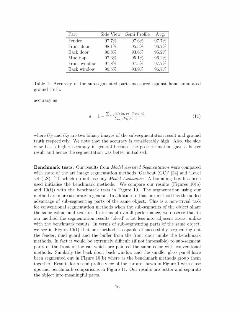
Table 1: Accuracy of the sub-segmented parts measured against hand annotatedground truth.

accuracy as

a = 1−∑

u, v |UR(u, v)−UG(u, v)|∑u, v UG(u, v) (11)

where UR and UG are two binary images of the sub-segmentation result and groundtruth respectively. We note that the accuracy is considerably high. Also, the sideview has a higher accuracy in general because the pose estimation gave a betterresult and hence the segmentation was better initialised.

Benchmark tests. Our results from Model Assisted Segmentation were comparedwith state of the art image segmentation methods ‘Grabcut (GC)’ [24] and ‘Levelset (LS)’ [11] which do not use any Model Assistance. A bounding box has beenused initialise the benchmark methods. We compare our results (Figures 10(b)and 10(f)) with the benchmark tests in Figure 10. The segmentation using ourmethod are more accurate in general. In addition to this, our method has the addedadvantage of sub-segmenting parts of the same object. This is a non-trivial taskfor conventional segmentation methods when the sub-segments of the object sharethe same colour and texture. In terms of overall performance, we observe that inour method the segmentation results ‘bleed’ a lot less into adjacent areas, unlikewith the benchmark results. In terms of sub-segmenting parts of the same object,we see in Figure 10(f) that our method is capable of successfully segmenting outthe fender, mud guard and the buffer from the front door unlike the benchmarkmethods. In fact it would be extremely difficult (if not impossible) to sub-segmentparts of the front of the car which are painted the same color with conventionalmethods. Similarly the back door, back window and the smaller glass panel havebeen segmented out in Figure 10(b) where as the benchmark methods group themtogether. Results for a semi-profile view of the car are shown in Figure 1 with closeups and benchmark comparisons in Figure 11. Our results are better and separatethe object into meaningful parts.

16

6 Discussion

The Model Assisted Segmentation method described in this paper can segment partsof a known 3D object from a given image. It performs better than the state of theart and can segment (and separate) parts that have similar pixel characteristics.We present our results on images of cars. The highly reflective surfaces of carsmake the pose estimation as well as the segmentation tasks more difficult than withnon-reflective objects.

We note that a close initialisation curve obtained from the 3D pose estimationsignificantly improves the performance of contour detection, and hence the imagesegmentation. However, the presence of reflections can deteriorate the quality ofthe results. We intend to explore avenues to make the process more robust in thepresence of reflections.

Acknowledgment. The authors wish to thank Stephen Gould and Hongdong Lifor the valuable feedback and advice. This work was supported by Control C=xpert.

References

[1] M. Arie-Nachimson and R. Basri. Constructing implicit 3d shape models for pose estimation.In ICCV, 2009.

[2] G. Bradski. The OpenCV Library. Dr. Dobb’s Journal of Software Tools, 2000.

[3] Brooks, R. A., and Binford, T. O. Geometric modelling in vision for manufacturing. InProceedings of the Society of Photo-Optical Instrumentation Engineers Conference on RobotVision, volume 281, pages 141–159, Washington, DC, USA, April 1981.

[4] V. Caselles, F. Catte, T. Coll, and F. Dibos. A geometric model for active contours in imageprocessing. Numerische Mathematik, 66(1):1–31, 1993.

[5] Roland T. Chin and Charles R. Dyer. Model-based recognition in robot vision. ACM Comput.Surv., 18(1):67–108, 1986.

[6] P. David, D. DeMenthon, R. Duraiswami, and H. Samet. SoftPOSIT: Simultaneous pose andcorrespondence determination. International Journal of Computer Vision, 59(3):259–284,2004.

[7] David A. Forsyth and Jean Ponce. Computer Vision: A Modern Approach. Prentice HallProfessional Technical Reference, 2002.

[8] B.K.P. Horn. Obtaining shape from shading information. In PsychCV75, pages 115–155,1975.

[9] M. Hutter and N. Brewer. Matching 2-D Ellipses to 3-D Circles with Application to VehiclePose Identification. In Image and Vision Computing New Zealand, 2009. IVCNZ’09. 24thInternational Conference, pages 153–158, 2009.

[10] Henner Kollnig and Hans-Hellmut Nagel. 3d pose estimation by directly matching polyhedralmodels to gray value gradients. Int. J. Comput. Vision, 23(3):283–302, 1997.

[11] Chunming Li, Chenyang Xu, Changfeng Gui, and M.D. Fox. Level set evolution withoutre-initialization: a new variational formulation. In Computer Vision and Pattern Recognition,2005. CVPR 2005. IEEE Computer Society Conference on, volume 1, pages 430 – 436 vol. 1,june 2005.

17

[12] R. Malladi, J. Sethian, and B. Vemuri. Evolutionary fronts for topology-independent shapemodeling and recovery. Computer VisionECCV’94, pages 1–13, 1994.

[13] R. Malladi, J.A. Sethian, and B.C. Vemuri. Shape modeling with front propagation: A levelset approach. Pattern Analysis and Machine Intelligence, IEEE Transactions on, 17(2):158–175, 2002.

[14] Ravikanth Malladi. A topology-independent shape modeling scheme. PhD thesis, Universityof Florida, Gainesville, FL, USA, 1993. AAI9505796.

[15] F. Moreno-Noguer, V. Lepetit, and P. Fua. Pose priors for simultaneously solving alignmentand correspondence. Computer Vision–ECCV 2008, pages 405–418, 2008.

[16] JA Nelder and R. Mead. A simplex method for function minimization. The computer journal,7(4):308, 1965.

[17] M. Ozuysal, V. Lepetit, and P.Fua. Pose estimation for category specific multiview objectlocalization. In Conference on Computer Vision and Pattern Recognition, Miami, FL, June2009.

[18] W. A. Perkins. A model-based vision system for industrial parts. IEEE Trans. Comput.,27(2):126–143, 1978.

[19] Poje, J. F., and Delp, E. J. A review of techniques for obtaining depth information withapplications to machine vision. Technical report, Center for Robotics and Integrated Manu-facturing, Univ. of Michigan, Ann Arbor, 1982.

[20] Joseph Lee Rodgers and W. Alan Nicewander. Thirteen ways to look at the correlationcoefficient. The American Statistician, 42(1):pp. 59–66, 1988.

[21] B. Rosenhahn, T. Brox, D. Cremers, and H.P. Seidel. A comparison of shape matchingmethods for contour based pose estimation. Combinatorial Image Analysis, pages 263–276,2006.

[22] B. Rosenhahn, T. Brox, and J. Weickert. Three-dimensional shape knowledge for joint imagesegmentation and pose tracking. International Journal of Computer Vision, 73(3):243–262,2007.

[23] B. Rosenhahn, C. Perwass, and G. Sommer. Pose estimation of 3D free-form contours. Inter-national Journal of Computer Vision, 62(3):267–289, 2005.

[24] C. Rother, V. Kolmogorov, and A. Blake. Grabcut: Interactive foreground extraction usingiterated graph cuts. ACM Transactions on Graphics (TOG), 23(3):309–314, 2004.

[25] M. Rousson and N. Paragios. Shape priors for level set representations. Computer Visio-nECCV 2002, pages 416–418, 2002.

[26] Min Sun, Bing-Xin Xu, Gary Bradski, and Silvio Savarese. Depth-encoded hough voting forjoint object detection and shape recovery. In ECCV, Crete, Greece, 09/2010 2010.

[27] T.N. Tan and K.D. Baker. Efficient image gradient based vehicle localization. IEEE Tran-sactions on Image Processing, 9(8):1343–1356, 2000.

[28] M. Yachida and S. Tsuji. A versatile machine vision system for complex industrial parts.IEEE Trans. Comput., 26(9):882–894, 1977.

18