3D Geometry-Based UAV-MIMO Channel Modeling … Geometry...describe a specific propagation...

China Communications • December 201864

Keywords: UAV-MIMO; geometry-based model; channel characteristics; simulation model

I. INTRODUCTION

In recent years, due to the low cost and high flexibility, the unmanned aerial vehicles (UAVs) have been widely used in weather monitoring, forest fire detection, traffic con-trol, communication relay [1]. The UAV com-munication systems have gradually become a research hotspot, and it is necessary to es-tablish an accurate and reliable UAV channel model.

The research of the UAV channel model is still lacking, and the existing models can be roughly divided into two categories， de-terministic model and statistical model. The Ray-tracing model [2], [3] and finite-differ-ence time domain method (FDTD) [4] model are two kinds of common UAV deterministic models. Deterministic models usually have high precision, but require a large amount of actual data and long operational time to describe a specific propagation environment. Therefore, the universality of the deterministic models is limited. Statistical model contains

Abstract: A more general narrowband regu-lar-shaped geometry-based statistical model (RS-GBSM) combined with the line of sight (LoS) and single bounce (SB) rays for un-manned aerial vehicle (UAV) multiple-input multiple-output (MIMO) channel is proposed in this paper. The channel characteristics, including space-time correlation function (STCF), Doppler power spectral density (DPSD), level crossing rate (LCR) and aver-age fade duration (AFD), are derived based on the single sphere reference model for a non-isotropic environment. The corresponding sum-of-sinusoids (SoS) simulation models including both the deterministic model and statistical model with finite scatterers are also proposed for practicable implementation. The simulation results illustrate that the simulation models well reproduce the channel charac-teristics of the single sphere reference model with sufficient simulation scatterers. And the statistical model has a better approximation of the reference model in comparison with the deterministic one when the simulation trials of the stochastic model are sufficient. The effects of the parameters such as flight height, moving direction and Rice factor on the characteristics are also studied.

3D Geometry-Based UAV-MIMO Channel Modeling and SimulationRubing Jia1,2,3, Yiran Li2, Xiang Cheng2,*, Bo Ai1,3

1 State Key Laboratory of Rail Traffic Control and Safety, Beijing Jiaotong University, Beijing 100044, China2 State Key Laboratory of Advanced Optical Communication Systems and Networks, School of Electronics Engineering and Computer Science, Peking University, Beijing 100871, China3 School of electronic and information engineering of Beijing Jiaotong University, Beijing Jiaotong University, Beijing 100044, China* The corresponding author, email: [email protected]

Received: Mar. 1, 2018Revised: Apr. 3, 2018 Editor: Yong Zeng

COMMUNICATIONS THEORIES & SYSTEMS

China Communications • December 2018 65

statistics including level crossing rate (LCR) and average fade duration (AFD) were stud-ied in [14]. Nevertheless, the model in [14] is merely for the single-input single-output (SISO) channel, while the UAV-MIMO chan-nel is obviously more suitable for practicable application. [17] proposed a GBSM for A2G channel, but the architecture of the model had fairly complex six elements. A series of cylinder UAV-MIMO models including both the narrowband and wideband models with reduced complexity was proposed in [18]–[21], but they all assume that the elevation and azimuth angles are independent. A 3D double-cylinder RS-GBSM for non-isotropic UAV-MIMO channel were proposed in [22], and the second order statistics, including LCR and AFD, were derived under the 3D propa-gation environment. In order to consider the joint effect of the azimuth and elevation an-gles, a 3D single-sphere RS-GBSM based on the von Mises Fisher (VMF) distribution was proposed in [23] for the UAV-MIMO chan-nels and the space-time correlation function (STCF) under a 3D moving environment was derived. However, [23] was based on urban scenarios with the assumption that the line of sight component was blocked by obstacles. According to the actual measurements of the UAV in some environments such as overwater [5] and sub-urban [6], the LoS component is dominant and cannot be ignored, and the more general models remain to be proposed.

Because the reference model assumes that the scatterers are infinite and cannot be ap-plied in practice, it is especially important to propose the corresponding simulation models. In [10], deterministic and statistical sum-of-si-nusoids (SoS) simulation models based on two-ring model for MIMO mobile-to-mobile (M2M) fading channels were proposed. [24] proposed both the deterministic and statistical simulation models for non-isotropic scattering M2M scenarios. As for UAV-MIMO channels, there are very few simulation models. [25] proposed deterministic and statistical simu-lation models based on the narrowband sin-gle-cylinder UAV-MIMO reference model, but

non-geometrical statistical model (NGSM) and geometry-based statistical model (GBSM). [5], [6] and [7] proposed a wideband tapped delay line (TDL) model, which is a common kind of the NGSM and composed of the line of sight (LoS) component, a ground reflection, and up to seven intermittent multi-path components (MPCs). However the models in [5]–[8] are based on the measurement and have some de-gree of complexity. The regular-shaped geom-etry-based statistical models (RS-GBSMs) can do us a favor to study the channel character-istics and provide a reference for the channel measurements in the absence of a large num-ber of measured data for the UAV.

RS-GBSMs can greatly reduce the com-plexity of the channel model by assuming that the scatterers are uniformly distributed in the regular geometrical shapes such as circle, cylinder and ellipse. The RS-GBSMs are often used in cellular communication and vehi-cle-to-vehicle communication scenes, showing high accuracy and generality [9]–[13]. As a new scenario for communication systems, UAV moves in the three-dimensional (3D) space. The flight parameters such as height and moving directions have important effects on the statistical characteristics of channel, and thus there are more requirements on the new RS-GBSMs for UAV. [14]–[16] proposed two air to ground (A2G) models which as-sumed that the scatterers around the ground station were uniformly distributed within the truncated ellipsoidal-shaped scattering region, which is more complicated than the common regular shapes such as cylinders and spheres. Besides, the distribution of both the azimuth and elevation angles is completely derived from geometrical relations in [14]–[16]. In contrast, cylinder and sphere models are more realistic for the reason that the angles of arriv-al and departure are modeled by the specific statistical mathematical forms such as cosine and von Mises distributions. These common statistical distributions make it easier to derive the closed-form expressions for the channel characteristics and have shown good fit to the previously measured data. Then second order

In this paper, the au-thors proposed a nar-rowband single sphere UAV-MIMO channel model and two new corresponding SoS b a s e d s i m u l a t i o n models.


characteristics are also derived. In Section V, numerical simulations are discussed to verify the simulation models and the effects of the flight parameters on characteristics are also analysed. Finally, conclusions are drawn in Section VI.

II. GEOMETRY-BASED UAV-MIMO CHANNEL REFERENCE MODEL

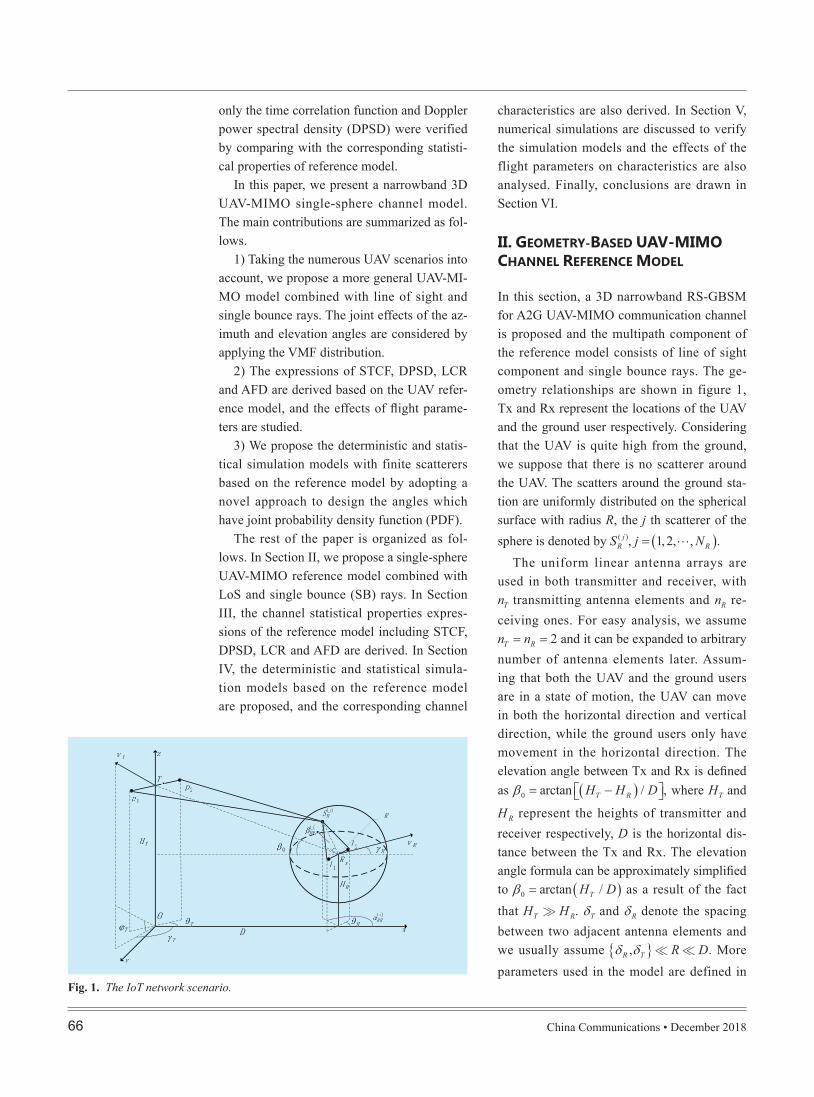
In this section, a 3D narrowband RS-GBSM for A2G UAV-MIMO communication channel is proposed and the multipath component of the reference model consists of line of sight component and single bounce rays. The ge-ometry relationships are shown in figure 1, Tx and Rx represent the locations of the UAV and the ground user respectively. Considering that the UAV is quite high from the ground, we suppose that there is no scatterer around the UAV. The scatters around the ground sta-tion are uniformly distributed on the spherical surface with radius R, the j th scatterer of the sphere is denoted by SR

( )j , j N= (1,2, , R ).The uniform linear antenna arrays are

used in both transmitter and receiver, with nT transmitting antenna elements and nR re-ceiving ones. For easy analysis, we assume n nT R= = 2 and it can be expanded to arbitrary number of antenna elements later. Assum-ing that both the UAV and the ground users are in a state of motion, the UAV can move in both the horizontal direction and vertical direction, while the ground users only have movement in the horizontal direction. The elevation angle between Tx and Rx is defi ned as β0 = −arctan / (H H DT R ) , where HT and

HR represent the heights of transmitter and receiver respectively, D is the horizontal dis-tance between the Tx and Rx. The elevation angle formula can be approximately simplifi ed to β0 = arctan /(H DT ) as a result of the fact that H HT R . δT and δR denote the spacing between two adjacent antenna elements and we usually assume δ δR T, R D. More parameters used in the model are defined in

only the time correlation function and Doppler power spectral density (DPSD) were verified by comparing with the corresponding statisti-cal properties of reference model.

In this paper, we present a narrowband 3D UAV-MIMO single-sphere channel model. The main contributions are summarized as fol-lows.

1) Taking the numerous UAV scenarios into account, we propose a more general UAV-MI-MO model combined with line of sight and single bounce rays. The joint effects of the az-imuth and elevation angles are considered by applying the VMF distribution.

2) The expressions of STCF, DPSD, LCR and AFD are derived based on the UAV refer-ence model, and the effects of fl ight parame-ters are studied.

3) We propose the deterministic and statis-tical simulation models with finite scatterers based on the reference model by adopting a novel approach to design the angles which have joint probability density function (PDF).

The rest of the paper is organized as fol-lows. In Section II, we propose a single-sphere UAV-MIMO reference model combined with LoS and single bounce (SB) rays. In Section III, the channel statistical properties expres-sions of the reference model including STCF, DPSD, LCR and AFD are derived. In Section IV, the deterministic and statistical simula-tion models based on the reference model are proposed, and the corresponding channel

Fig. 1. The IoT network scenario.

TT RR

z

y

xx

)(j)j)(j(RRRRRR((

D

)(j)j)(j(RS(S(

Tv

R

Rv0 R

TT

1p2p

1l

2llTH

RRH

xxT

xR

O )(j)j)(j(RR((


the l th ( 1,2, )l = ,nR antenna element to the center of the receiver antennas. Based on the assumption mentioned above n nT R= = 2, we define that ∆ =T Tδ / 2 and ∆ =R Rδ / 2.

III. CHANNEL CHARACTERISTICS OF THE 3D UAV-MIMO REFERENCE CHANNEL MODEL

In this section, considering the actual UAV communication scenes, several attractive statistic channel characteristics of the pro-posed 3D UAV-MIMO reference model for a non-isotropic scattering environment are derived, including the STCF, DPSD, LCR and AFD.

3.1 The STCF and DPSD

Assuming that the channel is wide-sense sta-tionary uncorrelated scattering (WSSUS), the STCF of arbitrary two sub-channels p l1 1→ , p l2 2→ can be written as

Rp l p l T R1 1 2 2, ( , , ) ,δ δ τ =E h t h t[ ( ) ( )]p l p l1 1 2 2

Ω Ωp l p l1 1 2 2

* +τ (4)

where h* ( )⋅ represents complex conjugate operations and E( )⋅ stands for mathematical expectation.

Table I.The expression of channel impulse response

(CIR) can be obtained by superimposing the LoS and SB ray,

h ( ) ( ) ( ),pl pl plt h t h t= +SBR LoS (1)

where,

⋅ ⋅

h t e

e e

plLoS

j f t j f t2 (cos cos cos sin sin ) 2 (cos cos )π γ β ϕ β ϕ π γ β

( )

T T T T R R

=KK

Ω

0 0 0

+pl

1+ −

j d p l2λπ ( , )

, (2)

h t eplSBR ( ) lim=

⋅

⋅

e

e j f t

j f t

2 cos( )cos cos sin sin

2 [cos( )cos ]

K

π α γ β

π α γ β ϕ β ϕ

Ω

T T T T

R R

+pl

1 NR

RR RR( ) ( )

TR TR TR( ) ( ) ( )

j j

→∞

j j j

−

− +

N1

R∑N

j=

.

R

1

j d p S d S l2λπ

( , ,R R R( ) ( ) ( )j j j)+ +( ) ψ

(3)where j2 = −1, λ is the is the carrier wave-length, the random phase shift ψ R

( )j is uniform-ly distributed over [−π π, ), Ωpl is the power

of the sub-channel p l− . K represents the Rice factor, which is the ratio of the receiving pow-er of the LoS component to that of the non-di-rect component.

Applying the sine law to the triangles and small angle approximation (i.e., sin x ≈ x and cos x ≈ 1 for small x), we can derive the following approximations for the AAoD a n d E A o D , α β αTR RR RR

( ) ( ) ( )j j j= ⋅(R Dcos / sin) ,

β β αTR RR( ) ( )j j≈ −0 R Dsin / . T h r o u g h t h e

calculation and simplification of geo-metric relations, we can get the distances d S l D R( R RR RR

( ) ( ) ( )j j j, / cos cos cos cos) ≈ +

− −

+

D R D

DT RR T RR1 1

T RR

cos cos ( cos

2sin )

β β α

β β α β

α0

0 0

( )j

( ) ( )j j

and d p S R D D( , sinR RR R R( ) ( ) 2 2j j) = ⋅ + +(( β )2

1 2 ),

where ∆ = + −T Tδ2T (n p1 2 ), ∆ = + −R R

δ2R (n l1 2 ),

D RR R RR RR R1= ∆ − ⋅ −cos cos( )β α θ( ) ( )i j ,

DT T T1= ∆ cosθ , DT T T2

= ∆ sinθ a n d

D RR RR RR R2= ⋅ −cos sin( )β α θ( ) ( )i j . The ∆T denotes

the distance from the p th ( 1,2, )p = ,nT an-tenna element to the center of the transmitter antennas. The ∆R denotes the distance from

Table I. Parameters used in the UAV model.Parameters Definition

θT, θR The orientations of the transmitting and receiving antenna arrays in the horizontal plane, respectively

vT, vR The velocities of transmitter and receiver, respectively

γT, γ R The azimuth angles of moving direction of transmitter and receiver, respectively

ϕT The elevation angle of moving direction of transmitter

αTR( )j , βTR

( )j

The azimuth angle of departure (AAoD) and elevation angle of depar-ture (EAoD) of the waves that impinge on the scatterers SR

( )j , respec-

tively

αRR( )j , βRR

( )j The azimuth angle of arrival (AAoA) and elevation angle of departure (EAoA) of the waves that impinge on the scatterers SR

( )j , respectively

ψ R( )j The random phase shift by SR

( )j

fT, fR The maximum Doppler shifts of transmitter and receiver, respectively

d p S( , )R( )j The distance between the transmitter antenna elements and the scat-

ters.

d S l( , )R( )j The distance between the scatters and the receiver antenna elements.


S f R e dp l p l

LoS LoS

11 2 2, 1 1 2 2( D p l p l) = ∫−∞

∞

, (τ τ) − j f2π τD , (11)

S f R e dSBR SBRp l p l11 2 2, 1 1 2 2

( D p l p l) = ∫−∞

∞

, (τ τ) − j f2π τD . (12)

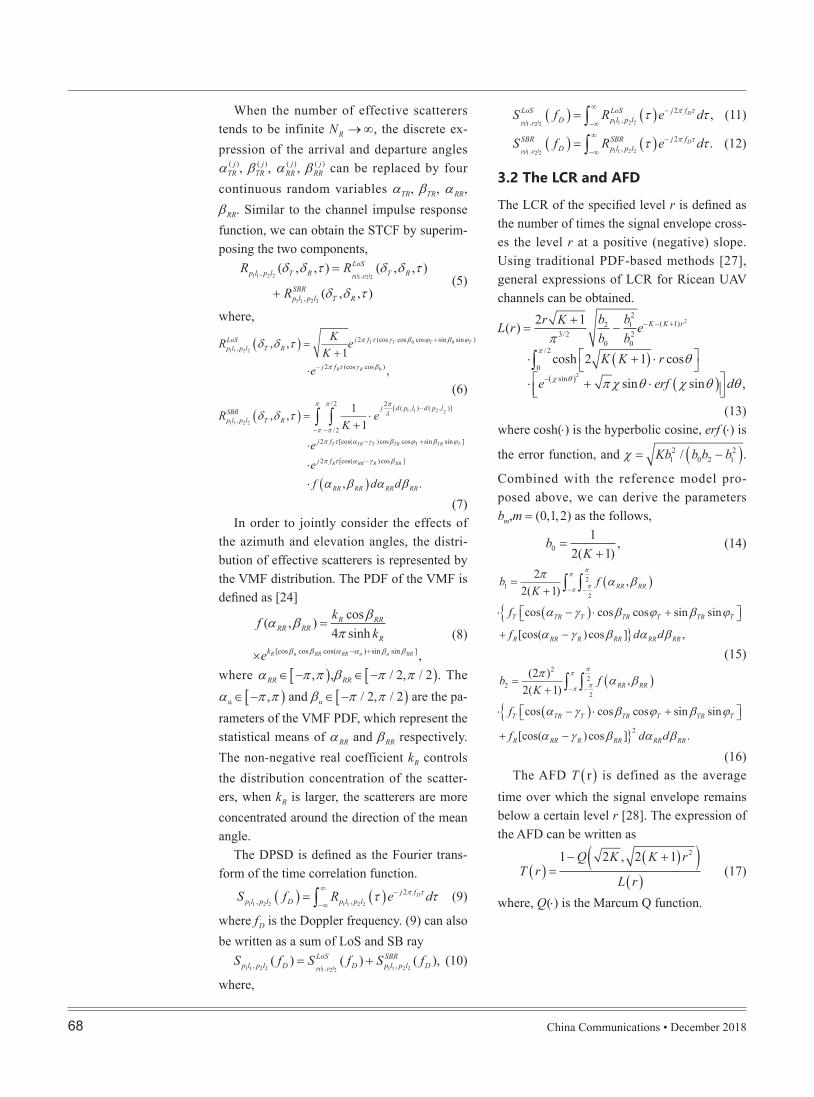
3.2 The LCR and AFD

The LCR of the specified level r is defined as the number of times the signal envelope cross-es the level r at a positive (negative) slope. Using traditional PDF-based methods [27], general expressions of LCR for Ricean UAV channels can be obtained.

L r e( ) = −

⋅ + ⋅

⋅ + ⋅∫

2 1

0

π

e erf d

r K

/2

−

π

(

cosh 2 1 cosχ θsin

3/2 2

+

)2

b bb bK K r

π χ θ χ θ θ

0 0

2 1

(sin sin ,

2− − +

)

K K r( 1)

(

2

θ

) (13)where cosh( )⋅ is the hyperbolic cosine, erf ( )⋅ is

the error function, and χ = −Kb b b b1 0 2 12 2/ ( ).

Combined with the reference model pro-posed above, we can derive the parameters bm,m = (0,1,2) as the follows,

b0 =2( 1)K

1+

, (14)

⋅ − ⋅ +

b f

+ −

1

f

f d d

=

T TR T TR T TR T

R RR R RR RR RR[cos( )cos ] ,

2( 1)

cos cos cos sin sin

K2π

α γ β α β

(+

α γ β ϕ β ϕ

∫ ∫−

π

π −

π2π

)2

(α βRR RR,

)

(15)

⋅ − ⋅ +

b f

+ −

2

f

f d d

T TR T TR T TR T

=

R RR R RR RR RR[cos( )cos ] .

2( 1)

cos cos cos sin sin

(2 )Kπ

α γ β α β

(+

α γ β ϕ β ϕ

2

∫ ∫−

π

π −

π2

)

π2

(α βRR RR

,

2

)

(16)The AFD T (r) is defined as the average

time over which the signal envelope remains below a certain level r [28]. The expression of the AFD can be written as

T r( ) =1 2 , 2 1− +Q K K r(

L r( )( ) 2 )

(17)

where, Q( )⋅ is the Marcum Q function.

When the number of effective scatterers tends to be infinite NR → ∞, the discrete ex-pression of the arrival and departure angles αTR

( )j , βTR( )j , αRR

( )j , βRR( )j can be replaced by four

continuous random variables αTR, βTR, αRR, βRR. Similar to the channel impulse response function, we can obtain the STCF by superim-posing the two components,

R Rp l p l T R T R1 1 2 2 ,,

+

( , , ) ( , , )δ δ τ δ δ τ

Rp l p l T RSBR

1 1 2 2, ( , , )δ δ τ

=p l p l

LoS

11 2 2 (5)

where,

R ep l p l T RLoS1 1 2 2, (δ δ τ, , ) =

⋅e− j f

K2 (cos cos )π τ γ β

K+R R

1j f2 (cos cos cos sin sin )π τ γ β ϕ β ϕT T T T

0 ,

0 0+

(6)

R ep l p l T RSBR

1 1 2 2, (δ δ τ, , ) = ⋅

⋅

⋅

⋅

ee

f d d

− −

π π

∫ ∫π π

j f

j f

(

2 [cos( )cos ]

2 [cos( )cos cos sin sin ]π τ α γ β ϕ β ϕ

π τ α γ β

α β α β

/2

T TR T TR T TR T

R RR R RR

RR RR RR RR

/2 K

, .

1+1

− +

)

−

j d p l d p l2λπ [ ( , ) ( , )]1 1 2− 2

(7)In order to jointly consider the effects of

the azimuth and elevation angles, the distri-bution of effective scatterers is represented by the VMF distribution. The PDF of the VMF is defined as [24]

×

f

e

( , )

k

α β

R u RR RR u u RR[cos cos cos( ) sin sin ]

RR RR

β β α α β β

=4 sinhkπR RRcos

− +

βkR

, (8)

where α π πRR ∈ −[ , ),β π πRR ∈ −[ / 2, / 2). The α π πu ∈ −[ , ) and β π πu ∈ −[ / 2, / 2) are the pa-rameters of the VMF PDF, which represent the statistical means of αRR and βRR respectively. The non-negative real coefficient kR controls the distribution concentration of the scatter-ers, when kR is larger, the scatterers are more concentrated around the direction of the mean angle.

The DPSD is defined as the Fourier trans-form of the time correlation function.

S f R e dp l p l D p l p l1 1 2 2 1 1 2 2, ,( ) = ∫−∞

∞(τ τ) − j f2π τD (9)

where fD is the Doppler frequency. (9) can also be written as a sum of LoS and SB ray

S f S f S fp l p l D D p l p l D1 1 2 2 , 1 1 2 2, ,( ) ( ) ( ),= +p l p l

LoS SBR

11 2 2 (10)

where,


sonable complexity. Based on the discussion of geometric relations in the reference model, it can be learned that the DoAs can be repre-sented by the AoAs, so only the set of AoAs α βRR RR

( ) ( )j j, is studied here.

Different from other models such as cyl-inder-based models, whose azimuth and elevation angles are independent, the AAoA and EAoA of the sphere-based models have joint PDF. It is impossible to achieve the cor-responding angles set by using the inverse function of the distribution function directly. In this particular case we have adopted a novel approach combined with the traditional mod-ified method of equal area (MMSE) method. That is to say, the AAoA is segmented into several subintervals firstly. The main steps are as follows

1) Divide the angle equally into Nα parts firstly.

Because the AAoA αRR( j ) is uniformly distributed

over [ , )−π π , we can define the random variable

as α π πRR( j ) = − + ⋅ −2 1 / 2 /( j N) α, j N= 1,2,..., α

Then we have Na intervals [− − +π π π, 2 / Nα ), [ 2 / , 4 / )− + − +π π π πN Nα α … , [π π π− 2 / ,Nα ).

2) Integrate the VMF PDF at each interval above, and the cumulative distribution function (CDF) sequence of the Na intervals is represented by CDF j( ), j 1,2,...,= Nα,which can be obtained

as CDF j f d d( ) = ∫ ∫−

π

π

/2

/2 − +

− +

π

π

2 1

2

πNπ

⋅ −N

α(

⋅

α

j

j ) (α β α βRR RR RR RR, ) .

3 ) C o m b i n e d w i t h t h e t r a d i t i o n -a l M M S E m e t h o d [ 1 1 ] , t h e E A o A β π π

RR( j k, ) ∈ −[ / 2, / 2) c a n b e d e f i n e d a s

( 1 / 2) / ,k N f d d− =β β α∫−

β

π

RR(

/2

j k, )

RR RR| (α β α βRR RR RR RR) ,

where fβ αRR RR| (α βRR RR, ) is the conditional

VMF PSD given that the AAoA αRR( j ) is known.

So we can get the expression of the EAoA

that βRR( , ) 1j k = Fβ α

−RR RR|

k −N1 / 2

β

，k N= 1,2,..., β,

where Fβ α−RR RR

1| ( )⋅ is the inverse function of

fβ αRR RR| (α βRR RR, ). The formula can be further

expressed as

IV. NEW SIMULATION MODELS FOR 3D UAV-MIMO CHANNELS

Because the reference model assumes that the scatterers are infinite, which prevents the practical implementation, the simulation mod-els with finite numbers of scaterers is needed [11]. The SoS simulation model is a kind of common simulation models using several sine waves to fit the channel, which can effectively reduce the computation. In this section, we propose both the deterministic and statistical simulation models for the non-isotropic scat-tering environment based on the UAV refer-ence model above. The channel characteristics of the simulation model are also derived to reproduce those of reference model.

4.1 New deterministic simulation model

The deterministic simulation model defines only the phases shift ψ R

( )j as random variables and the statistical channel characterises of the simulation model can be obtained through one simulation trial. The CIR of the deterministic simulation model can be get by the superposi-tion of LOS and SB ray,

h ( ) ( ) ( )

pl pl plt h t h t= +SBR LOS (18)

where,

h t e

plLoS ( ) =

⋅

⋅

ee

−

j f t2 (cos cos cos sin sin )

j f t

KKπ γ β ϕ β ϕ

2 (cos cos )π γ β

Ω

T T T T

+

R R

pl

1j d p l2

λπ ( , )

0 0

0 ,

+ (19)

h t e

plSBR ( ) lim=

⋅

⋅e

ej f t

j f t2 cos( )cos cos sin sin

2 [cos( )cos ]

K

π α γ β

π α γ β ϕ β ϕ

Ω

T T T T

R R

+pl

1 N

R

RR RR( ) ( )

TR TR TR( ) ( ) ( )

j j

→∞

j j j

−

− +

N1

R

∑N

j=

.

R

1

j d p S d S l2λπ

( , ,R R R( ) ( ) ( )j j j)+ +( ) ψ

(20)The sets of AoDs

α βTR TR

( ) ( )j j, and AoAs α βRR RR

( ) ( )j j, are designed to be discrete, which

is different from the continuous random vari-ables α βTR TR, and α βRR RR, in the reference

model, so that the simulation model can re-alistically reproduce the expected statistical characteristics of the reference one with rea-


the simulation, they cannot reflect the actual channel. To better simulate the fading process, the deterministic simulation model can be modifi ed into a statistical simulation model by defining the AoAs as random variables. The statistical channel characterises of the simu-lation model vary in each simulation trial. By averaging the suffi cient number of simulation trials, they will converge to those of the refer-ence model [10].

There are still three main steps and the fi rst two steps are similar to the deterministic mod-el.

1) Divide the horizontal angle equal-ly into Nα parts firstly. Similar to the de-terminis t ic s imulat ion model , we can def ine the random var iab le AAoA as a n NˆRR

(n) = − + ⋅ −π π2 1 / 2 /( ) α, n N= 1,2,..., α.2) Calculate the VMF PSD integral of each

interval and we can get the CDF sequence of the Nα integrals that can be obtained as

CDF n f d d( ) = ∫ ∫−

π

π

/2

/2 − +

− +

π

π

2 1

2

πNπ

⋅ −N

α(

⋅n

n

α

) (α β α βRR RR RR RR, ) .

3) Different from the deterministic simula-tion model, random variable σ β is introduced

in this step so that βRR( )n varies with differ-

ent simulation trials. The βRR( )n is defined as

βRR( ) 1n = =F s Nβ α β

−RR RR|

s + −σNβ

β

1 / 2, 1,2, , ,

where σ β is uniformly distributed over [ 1 / 2,1 / 2)− .

In this way, we fi nally get the deterministic and statistical simulation models. Similar to the derivation of the reference model channel characteristics, we extract the STCF, PSD, LCR and AFD of both the deterministic and statistical simulation model. The specifi c deri-vation process is no longer given as the length limit and the comparison between the refer-ence model and the two simulation models will be given in the next section.

V. NUMERICAL SIMULATION AND ANALYSIS

In this Section, we give the simulation results

∫ ∫

k

−

β

π

−

RR(

N CDF j

/2

j k,

1 / 2 1

β)

− +

− +

π

π

=

2 1

2

πNπ

⋅ −N

α(

⋅

α

j

j ) f d d

( )

(α β α βRR RR RR RR, .)

4.2 New statistical simulation model

It is fast and easy to implement deterministic simulation model, however, because their scatterers are placed in a specific position in

Fig. 2. The effect of the Ricean factor and simulation scatterers on the normalized time correlation function.

Fig. 3. Comparison of the normalized space correlation of the transmitter derived from the reference model and two simulation models with different VMF PSD pa-rametersn kR.

0 1 2 3 4 5

0.75

0.8

0.85

0.9

0.95

1

Nor

mal

ized

Tim

e C

orre

latio

n

deterministicrefstochastic

Nαα=Nββ=50, K=10

Nα=Nβ=50, K=5

Nαα=Nββ=10, K=3

Nαα=Nβββ=50, K=3=50, K=3=50, K=3=50, K=3

0 10 20 30 40 50 60 70 80 90δ

T/λ

0.1

0.2

0.3

0.4

0.5

0.6

0.7

0.8

0.9

1

Nor

mal

ized

Spa

ce C

orre

latio

n

referencedeterministicstatistical

kkR=0.=0.55

kkR=3=3=3=3=3=3=3

kkR=5=5


Because the parameter kR controls the distri-bution concentration of the scatterers, when kR is larger, the scatterers are more concentrated around the direction of the mean angle and thus the space correlation increases. By com-paring the figure 3 and figure 4, we can see that the spatial correlation of the receiver is signifi cantly smaller than that of the transmit-

of the reference model, deterministic simula-tion model and statistical simulation model. The STCF, DPSD, LCR and AFD are present-ed to verify the simulation models and analyse the effect of various parameters. Because the channel characteristics of the statistical sim-ulation model change with each simulation trial, to avoid the judgment of the reliability and practicability of the model, we average the multiple simulation results and the number of the simulation times is 50.

Combining with the actual UAV commu-nication scenes, the simulation parameters are set as follows, D m= 500 , R m= 10 , θ πT = / 3, θ πR = 2 / 3, β π0 = / 4, γ πT = / 6, ϕ πT = /12, γ πR = /12 , v m sT = 100 / , v m sR = 10 / , t h e VMF PDF parameters α πu = / 6, β πu = / 6, k = 0.5, the Ricean factor K = 5, the number of simulation scatters N Nα β= = 50.

We can obtain the the normalized time-CFs in fi gure 2 by changing the Ricean factor K = 3,5,10 and the number of scatterers

N Nα β= = 10,30,50. Figure 2 shows that the time correlation increases as K grows. It can be easily explained that, when K increases, the LoS component becomes more dominant and the influence of the change of scattering environment becomes smaller, which results in the time stability increase of the UAV chan-nel. What’s more, it can be seen that, when the number of simulation scatterers increases, the simulation model can better reproduce the statistical characteristics of the reference model, which also proves the validity of the two simulation models. Sufficient number of simulation scatterers is needed for a good ap-proximation. When the number of simulation scatterers is the same, the statistical model is more approximate to the reference model than the deterministic channel model with suffi cient simulation trials.

Figure 3 and 4 show the space correla-tion of the transmitter and receiver respec-tively. Changing the VMF PDF parameter kR = 0.5,3,5, we can observe that the spatial

correlation increases with the growth of kR.

Fig. 4. Comparison of the normalized space correlation of the receiver derived from the reference model and two simulation models.

0 0.5 1 1.5 2δ

R/λ

0.1

0.2

0.3

0.4

0.5

0.6

0.7

0.8

0.9

1

Nor

mal

ized

Spa

ce C

orre

latio

n


kRR=0.5kRR=3

kRR=5

Fig. 5. The Doppler power spectra characteristic for the UAV-MIMO channel model. The curves are obtained by varying the parameters of moving direction γ ϕT T, .

-800 -600 -400 -200 0 200 400 600 800

10

20

30

40

50

60

70

Dop

pler

Pow

er S

pect

rum

Den

sity


γγ TT=ππ /12,/12,φφTT=π /12

γγ TT=ππ /6/6,,φφTT==π /3

γγ T=ππ /6/6,,φφT==π /6


DPSD in fi gure 5. Varying the moving direc-tion of the UAV, we can see that the moving direction of UAV has a great infl uence on the Doppler power spectrum. γ π ϕ πT T= /6 = /3， is the set of statistical means of the PDF of AAoA and EAoA, which represents the con-centrated direction of the scatterers. The Dop-pler energy is more concentrated when mov-ing towards the direction where the scatterers are concentrated. When the UAV moves in other directions, the doppler power spectrum expands obviously.

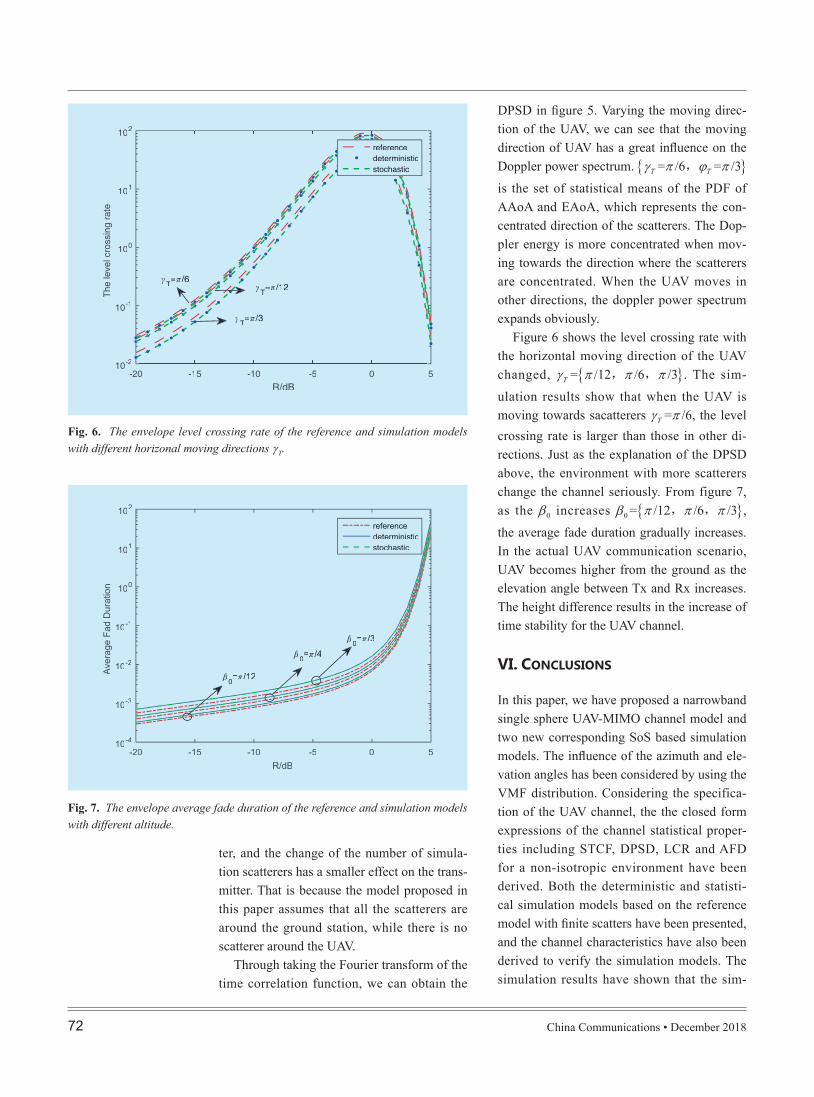
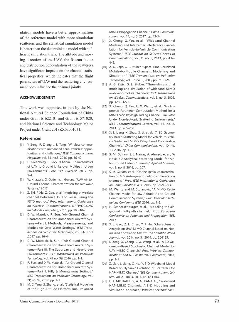
Figure 6 shows the level crossing rate with the horizontal moving direction of the UAV changed, γ π π πT = /12 /6 /3 ，， . The sim-ulation results show that when the UAV is moving towards sacatterers γ πT = /6, the level crossing rate is larger than those in other di-rections. Just as the explanation of the DPSD above, the environment with more scatterers change the channel seriously. From figure 7, as the β0 increases β π π π0 = /12 /6 /3 ，， , the average fade duration gradually increases. In the actual UAV communication scenario, UAV becomes higher from the ground as the elevation angle between Tx and Rx increases. The height difference results in the increase of time stability for the UAV channel.

VI. CONCLUSIONS

In this paper, we have proposed a narrowband single sphere UAV-MIMO channel model and two new corresponding SoS based simulation models. The infl uence of the azimuth and ele-vation angles has been considered by using the VMF distribution. Considering the specifica-tion of the UAV channel, the the closed form expressions of the channel statistical proper-ties including STCF, DPSD, LCR and AFD for a non-isotropic environment have been derived. Both the deterministic and statisti-cal simulation models based on the reference model with fi nite scatters have been presented, and the channel characteristics have also been derived to verify the simulation models. The simulation results have shown that the sim-

ter, and the change of the number of simula-tion scatterers has a smaller effect on the trans-mitter. That is because the model proposed in this paper assumes that all the scatterers are around the ground station, while there is no scatterer around the UAV.

Through taking the Fourier transform of the time correlation function, we can obtain the

Fig. 6. The envelope level crossing rate of the reference and simulation models with different horizonal moving directions γT.

Fig. 7. The envelope average fade duration of the reference and simulation models with different altitude.

-20 -15 -10 -5 0 5R/dB

10-2

10-1

100

101

102

The

leve

l cro

ssin

g ra

te

referencedeterministicstochastic

γTT=π /6

γTT=π /12

γTT=π /3

-20 -15 -10 -5 0 5R/dB

10-4

10-3

10-2

10-1

100

101

102

Aver

age

Fad

Dur

atio

n

referencedeterministicstochastic

ββ00=ππ /1/122

ββ00=ππ /4/4ββ00=ππ /3/3


MIMO Propagation Channel,” China Communi-cations, vol. 14, no. 3, 2017, pp. 43-54.

[9] X. Cheng, Q. Yao, et al., "Wideband Channel Modeling and Intercarrier Interference Cancel-lation for Vehicle-to-Vehicle Communication Systems," IEEE Journal on Selected Areas in Communications, vol. 31 no. 9, 2013, pp. 434-448.

[10] A. G. Zajic, G. L. Stuber, “Space-Time Correlated Mobile-to-Mobile Channels: Modelling and Simulation,” IEEE Transactions on Vehicular Technology, vol. 57, no. 2, 2008, pp. 715-726.

[11] A. G. Zajic, G. L. Stuber, “Three-dimensional modeling and simulation of wideband MIMO mobile-to-mobile channels,” IEEE Transactions on Wireless Communications, vol. 8, no. 3, 2009, pp. 1260-1275.

[12] X. Cheng, Q. Yao, C. X. Wang, et al., “An Im-proved Parameter Computation Method for a MIMO V2V Rayleigh Fading Channel Simulator Under Non-Isotropic Scattering Environments,” IEEE Communications Letters, vol. 17, no. 2, 2013, pp. 265-268.

[13] X. L. Liang, X. Zhao, S. Li, et al., “A 3D Geome-try-Based Scattering Model for Vehicle-to-Vehi-cle Wideband MIMO Relay-Based Cooperative Channels,” China Communications, vol. 10, no. 13, 2016, pp. 1-2.

[14] S. M. Gulfam, S. J. Nawaz, A. Ahmed, et al., “A Novel 3D Analytical Scattering Model for Air-to-Ground Fading Channels,” Applied Sciences, vol. 6, no. 8, 2016, pp. 207.

[15] S. M. Gulfam, et al., "On the spatial characteriza-tion of 3-D air-to-ground radio communication channels," Proc. IEEE International Conference on Communications IEEE, 2015, pp. 2924-2930.

[16] M. Wentz, and M. Stojanovic, "A MIMO Radio Channel Model for Low-Altitude Air-to-Ground Communication Systems," Proc. Vehicular Tech-nology Conference IEEE, 2016, pp. 1-6.

[17] N. Schneckenburger, et al., "Modeling the air-ground multipath channel," Proc. European Conference on Antennas and Propagation IEEE, 2017.

[18] X. J. Gao, Z. L. Chen, Y. J. Hu, “Characteristic Analysis on UAV-MIMO Channel Based on Nor-malized Correlation Matrix,” The Scientific World Journal,, vol. 2014, no. 3, 2014, pp. 206185.

[19] L. Zeng, X. Cheng, C. X. Wang, et al., “A 3D Ge-ometry-Based Stochastic Channel Model for UAV-MIMO Channels,” Proc. Wireless Commu-nications and NETWORKING Conference, 2017, pp. 1-5.

[20] Z. Lian, L. Jiang, C. He, “A 3-D Wideband Model Based on Dynamic Evolution of Scatterers for HAP-MIMO Channel,” IEEE Communications Let-ters, vol. 21, no. 3, 2017, pp. 684-687.

[21] E. T. MICHAILIDIS, A. G. KANATAS, “Wideband HAP-MIMO Channels: A 3-D Modeling and Simulation Approach,” Wireless personal com-

ulation models have a better approximation of the reference model with more simulation scatterers and the statistical simulation model is better than the deterministic model with suf-ficient simulation trials. The altitude and mov-ing direction of the UAV, the Ricean factor and distribution concentration of the scatterers have significant impacts on the channel statis-tical properties, which indicates that the flight parameters of UAV and the scattering environ-ment both influence the channel jointly.

ACKNOWLEDGEMENT

This work was supported in part by the Na-tional Natural Science Foundation of China under Grant 61622101 and Grant 61571020, and National Science and Technology Major Project under Grant 2018ZX03001031.

References[1] Y. Zeng, R. Zhang, J. L. Teng, “Wireless commu-

nications with unmanned aerial vehicles: oppor-tunities and challenges,” IEEE Communications Magazine, vol. 54, no.5, 2016, pp. 36-42.

[2] E. Greenberg, P. Levy. “Channel Characteristics of UAV to Ground Links over Multipath Urban Environments” Proc. IEEE COMCAS, 2017, pp. 1-4.

[3] W. Khawaja, O. Ozdemir, I. Guvenc. “UAV Air-to-Ground Channel Characterization for mmWave Systems,” 2017.

[4] Z. Shi, P. Xia, Z. Gao, et al. “Modeling of wireless channel between UAV and vessel using the FDTD method,” Proc. International Conference on Wireless Communications, NETWORKING and Mobile Computing, 2015, pp. 100-104.

[5] D. W. Matolak, R. Sun, “Air–Ground Channel Characterization for Unmanned Aircraft Sys-tems—Part I: Methods, Measurements, and Models for Over-Water Settings,” IEEE Trans-actions on Vehicular Technology, vol. 66, no.1 ,2017, pp. 26-44.

[6] D. W. Matolak, R. Sun, “"Air-Ground Channel Characterization for Unmanned Aircraft Sys-tems—Part III: The Suburban and Near-Urban Environments,” IEEE Transactions on Vehicular Technology, vol. PP, no. 99, 2016, pp. 1-1.

[7] R. Sun, and D. W. Matolak, "Air-Ground Channel Characterization for Unmanned Aircraft Sys-tems—Part II: Hilly & Mountainous Settings," IEEE Transactions on Vehicular Technology, vol. PP, no. 99, 2017, pp. 1-1.

[8] M. C. Yang, S. Zhang, et al., “Statistical Modeling of the High Altitude Platform Dual-Polarized


BiographiesRubing Jia, graduate student with the School of electronic and information engineering, Beijing Jiaotong University. Her current research interests in-clude wireless communications and UAV channel modeling. Email: [email protected].

Yiran Li, graduate student with the School of Software and Mi-croelectronics, Peking Universi-ty. Her current research inter-ests include channel modeling and vehicular communications. Email: [email protected].

Xiang Cheng, professor with the School of Electronics Engi-neering and Computing Sci-ence, Peking University. His current research interests in-clude channel modeling, wire-less communications (vehicular communications and 5G), and

data analytics. Email: [email protected].

Bo Ai, professor with the School of electronic and infor-mation engineering, Beijing Ji-aotong University. His current research interests include the research and applications of channel measurement and channel modeling, dedicated

mobilecommunicationsforrailtrafficsystems.Email:[email protected].

munications, vol. 74, no. 2, 2014, pp. 639-664.[22] L. Zeng, X. Cheng, C. X. Wang, et al., “Second

Order Statistics of Non-Isotropic UAV Ricean Fading Channels,” Proc. IEEE Vehicular Technolo-gy Conference Fall, 2018, pp. 1-5.

[23] K. Jin, X. Cheng, X. Ge, et al., “Three Dimension-al Modeling and Space-Time Correlation for UAV Channelss,” Proc. IEEE Vehicular Technology Conference Fall, 2017, pp. 1-5.

[24] X. Cheng, C. X. Wang, D. I. Laurenson, et al., “New deterministic and stochastic simulation models for non-isotropic scattering mobile-to-mobile Rayleigh fading channels,” Wireless Commu-nications & Mobile Computing, vol. 11, no. 7, 2011, pp. 829-842.

[25] Y. Li, X. Cheng, “New deterministic and sta-tistical simulation models for non-isotropic UAV-MIMO channels,” Proc. International Con-ference on Wireless Communications and Signal Processing, 2017, pp. 1-6.

[26] Y. Yuan, X. Cheng, C. X. Wang, et al., “Space-Time Correlation Properties of a 3D Two-Sphere Model for Non-Isotropic MIMO Mobile-to-Mo-bile Channels,” Proc. IEEE Global Telecommuni-cations Conference, 2010, pp. 1-5.

[27] A. G. Zajic, G. L. Stiiber, T. G. Pratt, et al., “Enve-lope Level Crossing Rate and Average Fade Du-ration in Mobile-To-Mobile Fading Channels,” 2008, pp. 4446-4450.

[28] X. Cheng, C. X. Wang, H. Aggoune, et al., “En-velope Level Crossing Rate and Average Fade Duration of Nonisotropic Vehicle-to-Vehicle Ricean Fading Channels,” IEEE Transactions on Intelligent Transportation Systems, vol. 15, no. 1, 2014, pp. 62-72.

3D Geometry-Based UAV-MIMO Channel Modeling … Geometry...describe a specific propagation...

Documents

Transcript of 3D Geometry-Based UAV-MIMO Channel Modeling … Geometry...describe a specific propagation...