Frank Jenko

Max-Planck-Institut für Plasmaphysik, Garching Universität Ulm

HEPP Guest Lecture

Garching, 31 July 2013

An introduction to turbulence in

fusion plasmas I

Introductory remarks

This lecture series is meant to be an introduction; no prior knowledge of turbulence is required I will make an effort to make the material accessible to a wide range of scientists You are invited to ask questions at any time Lectures may explain, motivate, inspire etc., but they cannot replace individual study...

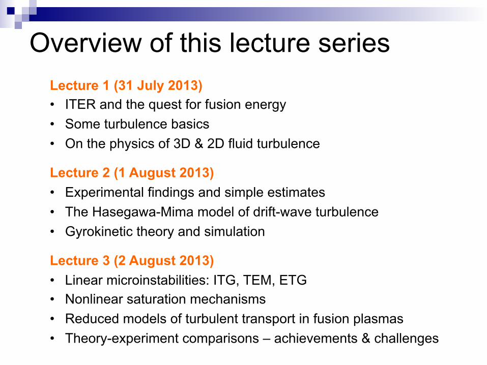
Overview of this lecture series Lecture 1 (31 July 2013) •  ITER and the quest for fusion energy •  Some turbulence basics •  On the physics of 3D & 2D fluid turbulence

Lecture 2 (1 August 2013) •  Experimental findings and simple estimates •  The Hasegawa-Mima model of drift-wave turbulence •  Gyrokinetic theory and simulation

Lecture 3 (2 August 2013) •  Linear microinstabilities: ITG, TEM, ETG •  Nonlinear saturation mechanisms •  Reduced models of turbulent transport in fusion plasmas •  Theory-experiment comparisons – achievements & challenges

ITER and the quest for fusion energy

Global electricity needs increase by a factor of 6 until 2100

Energy Modeling Forum 22: 100 models from 15 research groups (Clarke et al., 2009)

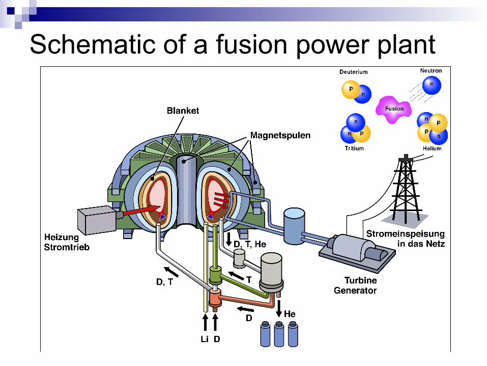
Schematic of a fusion power plant

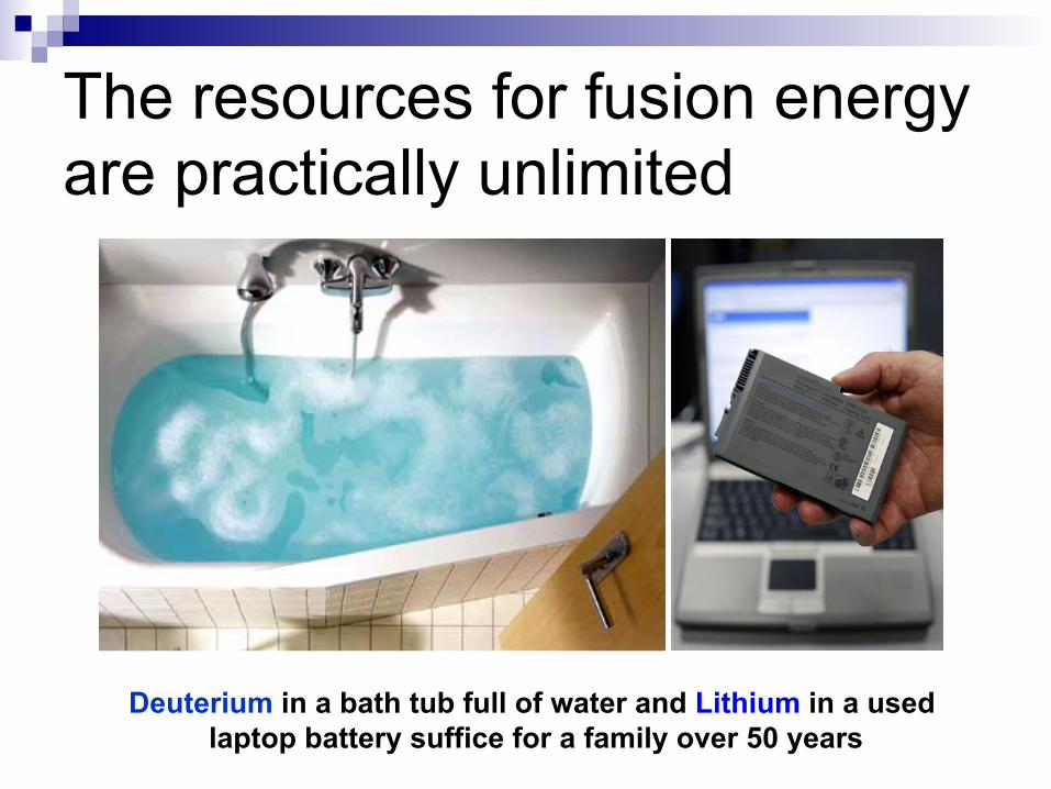
The resources for fusion energy are practically unlimited

Deuterium in a bath tub full of water and Lithium in a used laptop battery suffice for a family over 50 years

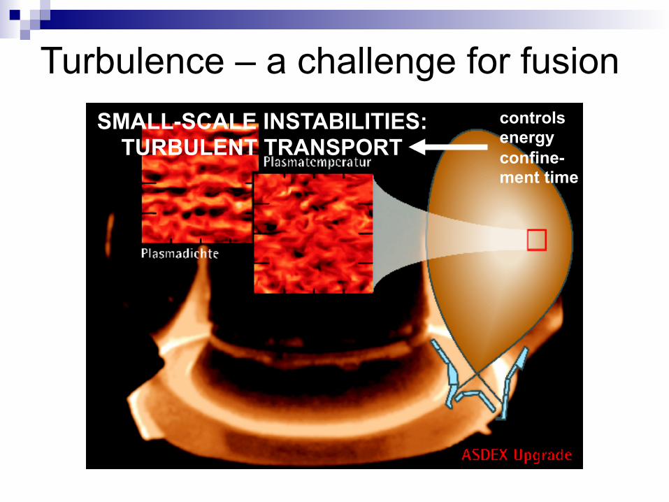
Turbulence – a challenge for fusion SMALL-SCALE INSTABILITIES:

TURBULENT TRANSPORT controls energy confine- ment time

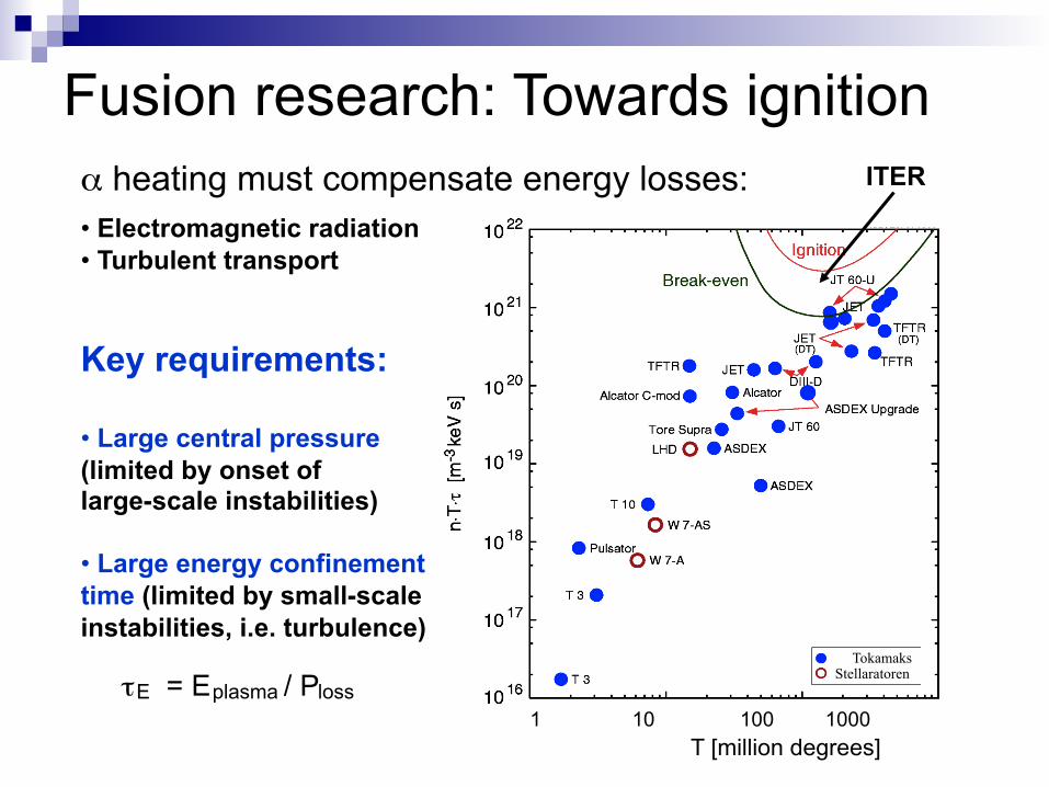
α heating must compensate energy losses:

•  Electromagnetic radiation •  Turbulent transport

Key requirements: •  Large central pressure (limited by onset of large-scale instabilities) •  Large energy confinement time (limited by small-scale instabilities, i.e. turbulence):

τ = E / P E plasma loss 1 10 100 1000

T [million degrees]

Tokamaks Stellaratoren

Fusion research: Towards ignition ITER

Progress in fusion

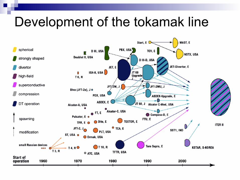
Development of the tokamak line

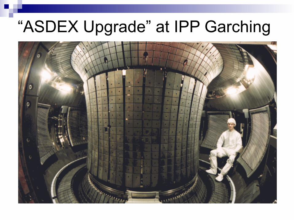
“ASDEX Upgrade” at IPP Garching

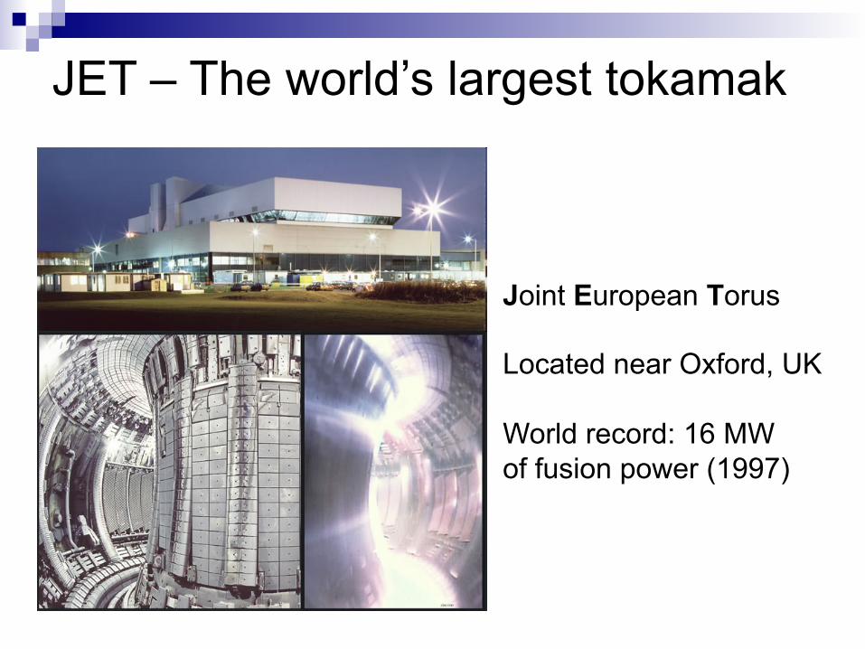
JET – The world’s largest tokamak

Joint European Torus Located near Oxford, UK World record: 16 MW of fusion power (1997)

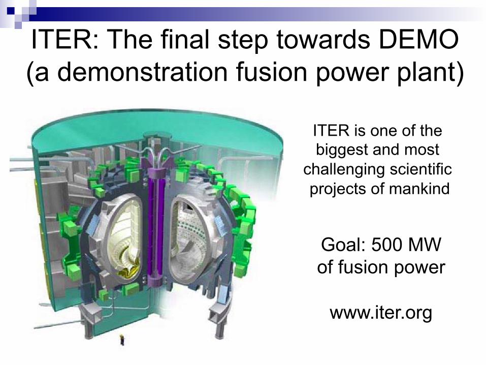
Goal: 500 MW of fusion power

www.iter.org

ITER: The final step towards DEMO (a demonstration fusion power plant)

ITER is one of the biggest and most

challenging scientific projects of mankind

Some turbulence basics

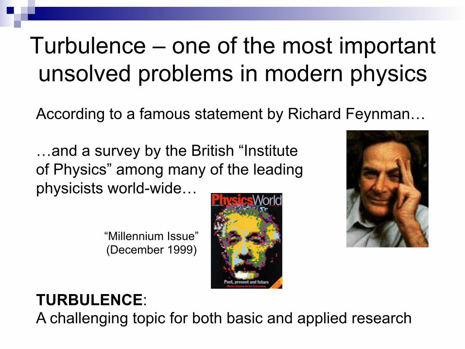
According to a famous statement by Richard Feynman… …and a survey by the British “Institute of Physics” among many of the leading physicists world-wide… TURBULENCE: A challenging topic for both basic and applied research

Turbulence – one of the most important unsolved problems in modern physics

“Millennium Issue” (December 1999)

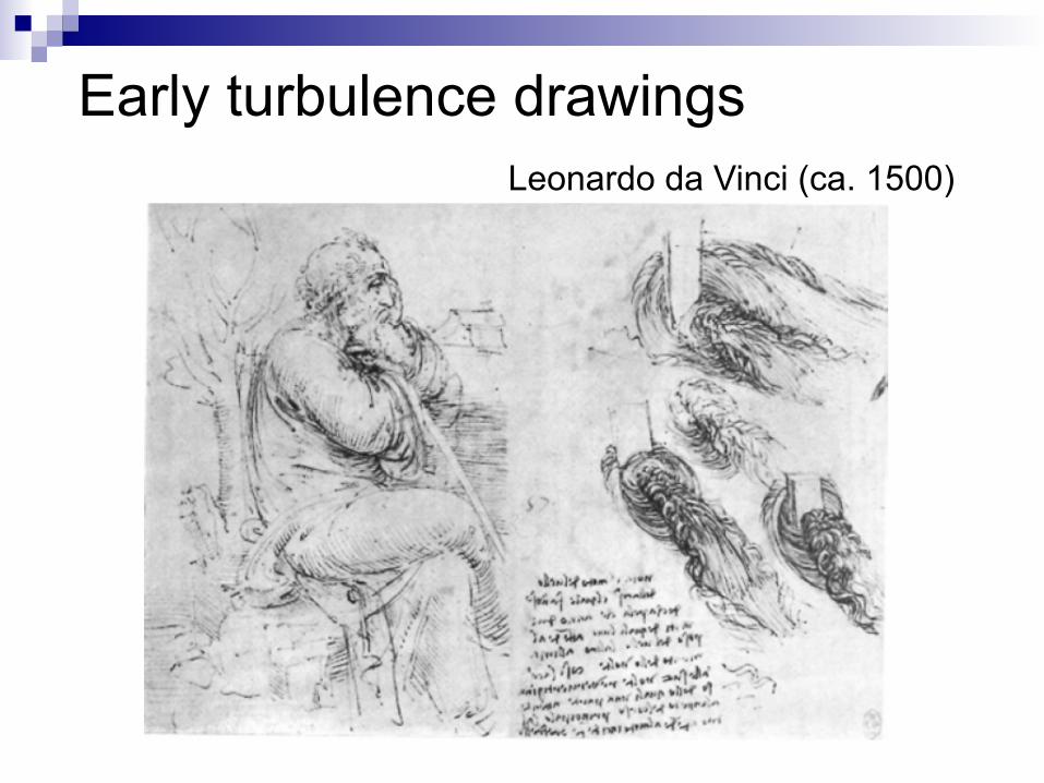
Early turbulence drawings Leonardo da Vinci (ca. 1500)

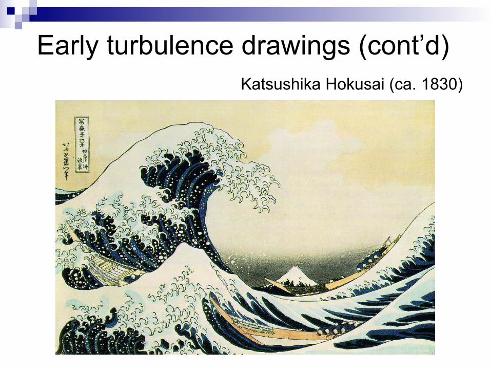
Early turbulence drawings (cont’d) Katsushika Hokusai (ca. 1830)

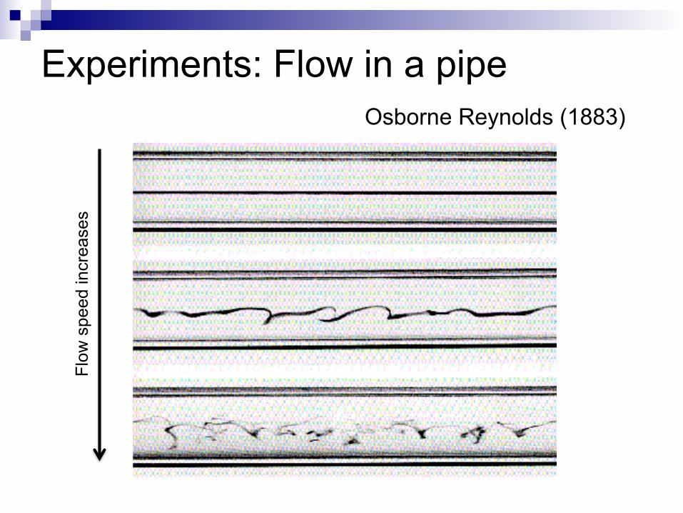
Experiments: Flow in a pipe Osborne Reynolds (1883)

Flow

spe

ed in

crea

ses

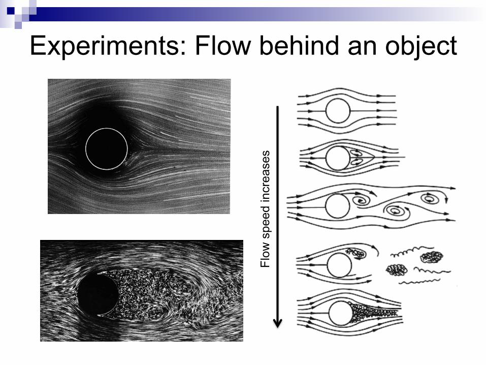
Fluid Flow Behind a Cylinder vs. R

R < 1

R ~ 5-40

R~100-200

R ~ 104

R ~ 106

Experiments: Flow behind an object

Flow

spe

ed in

crea

ses

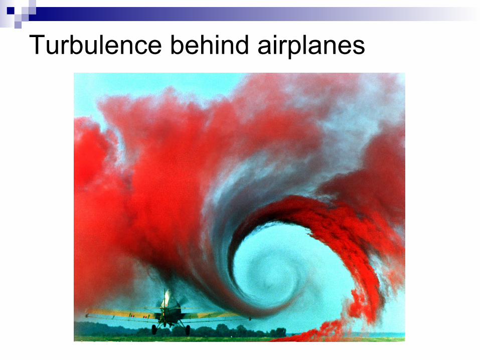
Turbulence behind airplanes

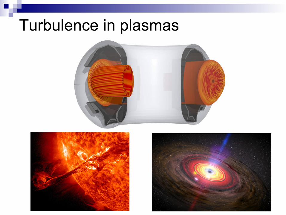
Turbulence in plasmas

What is turbulence then? Turbulence…

•  is an intrinsically nonlinear phenomenon

•  occurs (only) in open systems

•  involves many degrees of freedom

•  is highly irregular (chaotic) in space and time

•  often leads to a (statistically) quasi-stationary state far from thermodynamic equilibrium

These properties make it a very complicated problem – neither Dynamical Systems Theory nor Statistics applies!

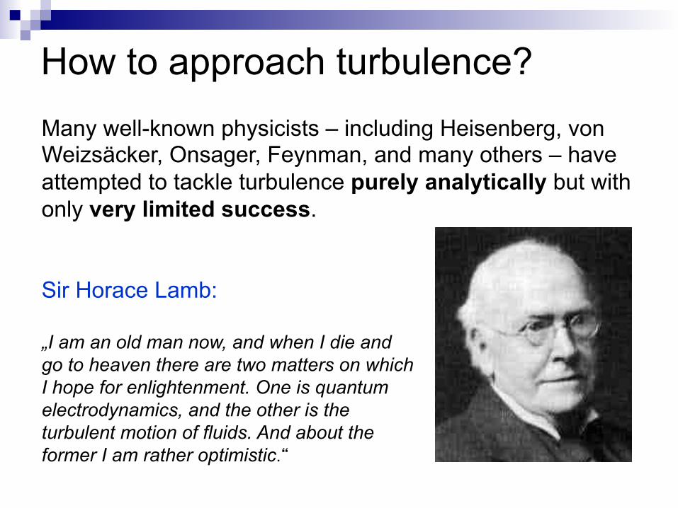
How to approach turbulence? Many well-known physicists – including Heisenberg, von Weizsäcker, Onsager, Feynman, and many others – have attempted to tackle turbulence purely analytically but with only very limited success. Sir Horace Lamb: „I am an old man now, and when I die and go to heaven there are two matters on which I hope for enlightenment. One is quantum electrodynamics, and the other is the turbulent motion of fluids. And about the former I am rather optimistic.“

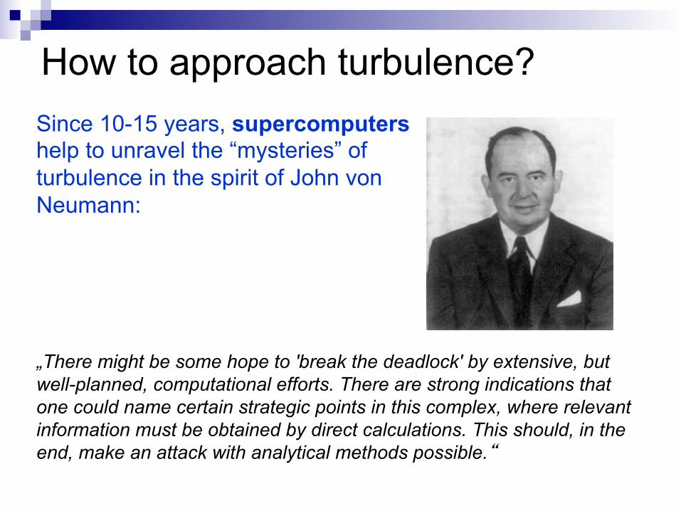
How to approach turbulence? Since 10-15 years, supercomputers help to unravel the “mysteries” of turbulence in the spirit of John von Neumann: „There might be some hope to 'break the deadlock' by extensive, but well-planned, computational efforts. There are strong indications that one could name certain strategic points in this complex, where relevant information must be obtained by direct calculations. This should, in the end, make an attack with analytical methods possible.“

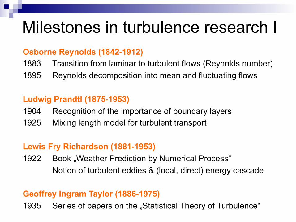
Milestones in turbulence research I Osborne Reynolds (1842-1912) 1883 Transition from laminar to turbulent flows (Reynolds number) 1895 Reynolds decomposition into mean and fluctuating flows Ludwig Prandtl (1875-1953) 1904 Recognition of the importance of boundary layers 1925 Mixing length model for turbulent transport Lewis Fry Richardson (1881-1953) 1922 Book „Weather Prediction by Numerical Process“

Notion of turbulent eddies & (local, direct) energy cascade Geoffrey Ingram Taylor (1886-1975) 1935 Series of papers on the „Statistical Theory of Turbulence“

Milestones in turbulence research II Werner Heisenberg (1901-1976) 1923 „Über Stabilität und Turbulenz von Flüssigkeitsströmen“

(PhD Thesis, LMU München, Advisor: Arnold Sommerfeld) 1948 Three papers on the statistical theory of turbulence Andrey Kolmogorov (1903-1987) 1941 K41 theory: dimensional analysis, -5/3 law (energy spectrum) 1962 K62 theory: scale invariance is broken, problem of intermittency Robert Kraichnan (1928-2008) 1957- Field-theoretic approach: Direct Interaction Approximation 1967 Inverse energy cascade in two-dimensional fluid turbulence

1973 Field-theoretic approach: Martin-Siggia-Rose formalism

Milestones in turbulence research III Steven Orszag (1943-2011) 1966 Eddy-Damped Quasi-Normal Markovian approximation 1969- Towards Direct Numerical Simulations via spectral methods 1972 First 3D DNS on a 323 grid by S. Orszag & G. Patterson

1948- Numerical weather prediction by J. von Neumann & J. Charney 1963 Large-Eddy Simulation techniques by J. Smagorinsky 1965 Fast Fourier Transform algorithm by J. Cooley & J. Tukey 1977 Cray-1 at the National Center for Atmospheric Research

2002 Largest 3D DNS to date on a 40963 grid by Y. Kaneda et al.

Some grand challenges •  Design airplanes, ships, cars etc. •  Predict weather & climate •  Unravel role of turbulence in space & astrophysics •  Predict performance of fusion devices like ITER

Some open problems beyond Homogeneous Isotropic Turbulence •  Effects of inhomogeneity, anisotropy, compressibility

(role of walls, drive, stratification, rotation etc.) •  From fluid to magneto-/multi-fluid to kinetic turbulence

Conceptual approach •  Ab initio simulations of complicated problems are not feasible •  Seek physics understanding to construct reliable minimal models

Turbulence: The bigger picture

On the physics of 3D fluid turbulence

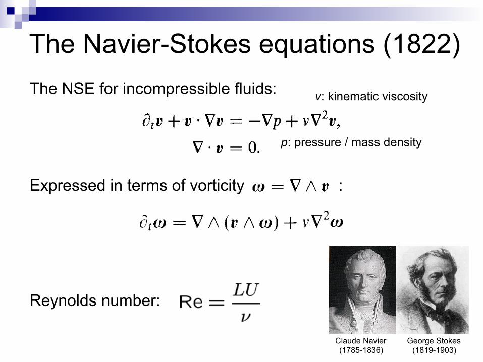
The Navier-Stokes equations (1822) The NSE for incompressible fluids: Expressed in terms of vorticity : Reynolds number:

ν: kinematic viscosity

p: pressure / mass density

Claude Navier (1785-1836)

George Stokes (1819-1903)

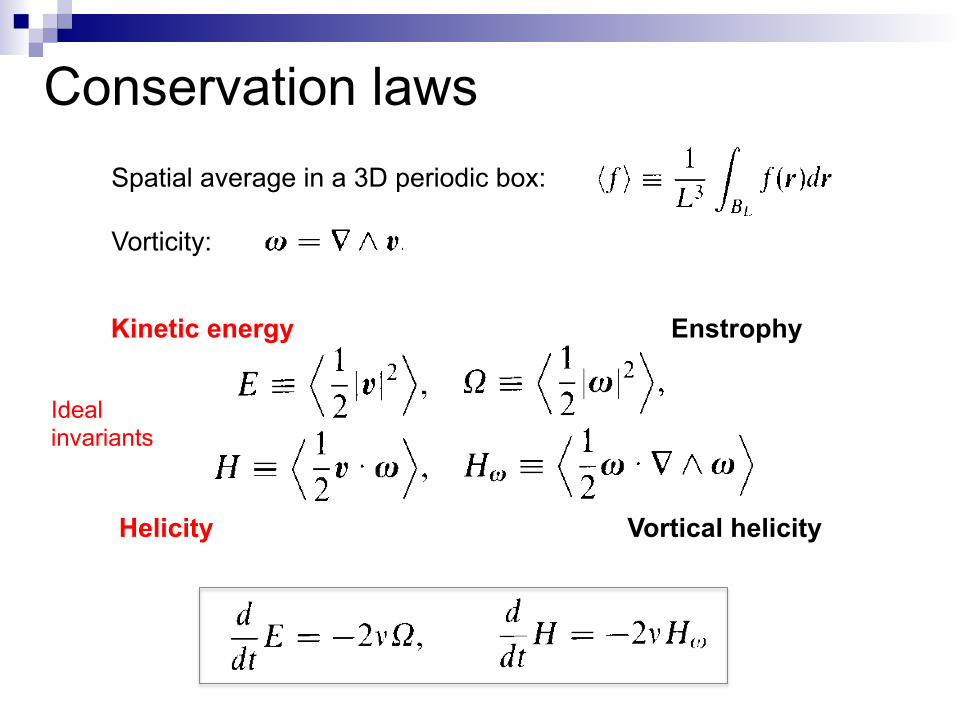
Conservation laws

Kinetic energy Enstrophy

Helicity Vortical helicity

Spatial average in a 3D periodic box: Vorticity:

Ideal invariants

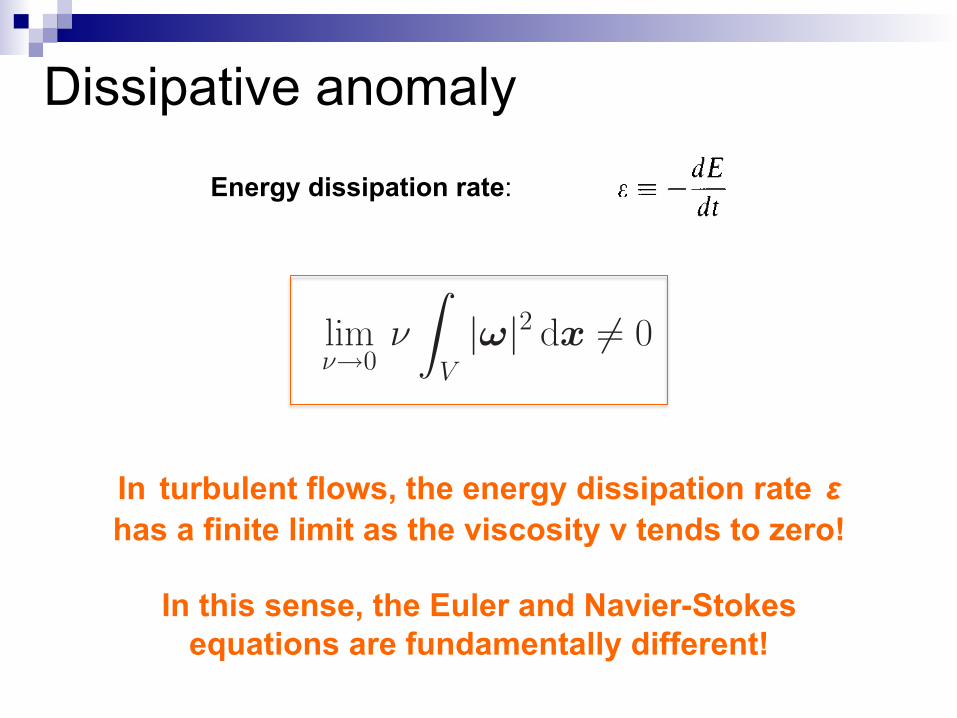
Dissipative anomaly

Energy dissipation rate:

An enclosed incompressible fluid

The power integral is:

and

with the vorticity

The zeroth law is:

Turbulence is a singular limit (a “dissipative anomaly”).

!(ut + u·!u) + !p = µ!2u + f and !·u = 0

d

dt

!

V

1

2|u|2 dx =

!

V

u·f dx " "

!

V

|!|2 dx

! = ! # u

lim!!0

"

!

V

|!|2 dx $= 0

! #

"

!#

ut + u·!u$

+ !p = µ!2u

%

!t + u·!! = ! ·!u + "!2!

u = uı̂ + v"̂ ! = (vx " uy)k̂ ! ! ·!u = 0

"air % 10"5

m2

s"1

1

!(ut + u·!u) + !p = µ!2u + f and !·u = 0

d

dt

!

V

1

2|u|2 dx =

!

V

u·f dx " "

!

V

|!|2 dx

! = ! # u

lim!!0

"

!

V

|!|2 dx $= 0

! #

"

!#

ut + u·!u$

+ !p = µ!2u

%

!t + u·!! = ! ·!u + "!2!

u = uı̂ + v"̂ ! = (vx " uy)k̂ ! ! ·!u = 0

"air % 10"5

m2

s"1

1

!(ut + u·!u) + !p = µ!2u + f and !·u = 0

d

dt

!

V

1

2|u|2 dx =

!

V

u·f dx " "

!

V

|!|2 dx

! = ! # u

lim!!0

"

!

V

|!|2 dx $= 0

! #

"

!#

ut + u·!u$

+ !p = µ!2u

%

!t + u·!! = ! ·!u + "!2!

u = uı̂ + v"̂ ! = (vx " uy)k̂ ! ! ·!u = 0

"air % 10"5

m2

s"1

1

!(ut + u·!u) + !p = µ!2u + f and !·u = 0

d

dt

!

V

1

2|u|2 dx =

!

V

u·f dx " "

!

V

|!|2 dx

! = ! # u

lim!!0

"

!

V

|!|2 dx $= 0

! #

"

!#

ut + u·!u$

+ !p = µ!2u

%

!t + u·!! = ! ·!u + "!2!

u = uı̂ + v"̂ ! = (vx " uy)k̂ ! ! ·!u = 0

"air % 10"5

m2

s"1

1

!(ut + u·!u) + !p = µ!2u + f and !·u = 0

d

dt

!

V

1

2|u|2 dx =

!

V

u·f dx " "

!

V

|!|2 dx

! = ! # u

lim"$0

"

!

V

|!|2 dx %= 0

! #

"

!#

ut + u·!u$

+ !p = µ!2u

%

!t + u·!! = ! ·!u + "!2!

u = uı̂ + v"̂ ! = (vx " uy)k̂ ! ! ·!u = 0

"air & 10!5

m2

s!1

1

u = k̂ ! !!

u = 0

d

dt

!!

1

2|!!|2 dxdy = ""

!!

#2 dxdy

d

dt

!!

1

2#2 dxdy = ""

!!

|!#|2 dxdy

d

dt

!!

F (#) dxdy = ""

!!

|!#|2F !!(#) dx

vx " uy = #2!

vx " uy = #2!

d

dt

!

V

1

2|u|2 dx =

!

V

u·f dx " "

!

V

|!|2 d

Saturday, March 16, 2013

In turbulent flows, the energy dissipation rate ε has a finite limit as the viscosity ν tends to zero!

In this sense, the Euler and Navier-Stokes

equations are fundamentally different!

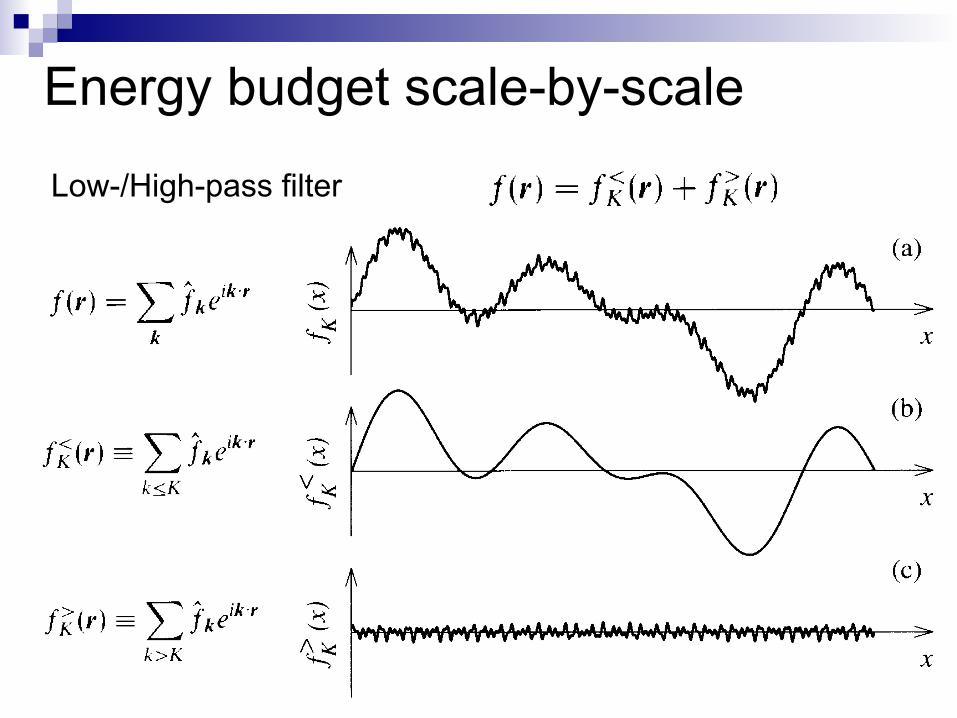
Energy budget scale-by-scale

Low-/High-pass filter

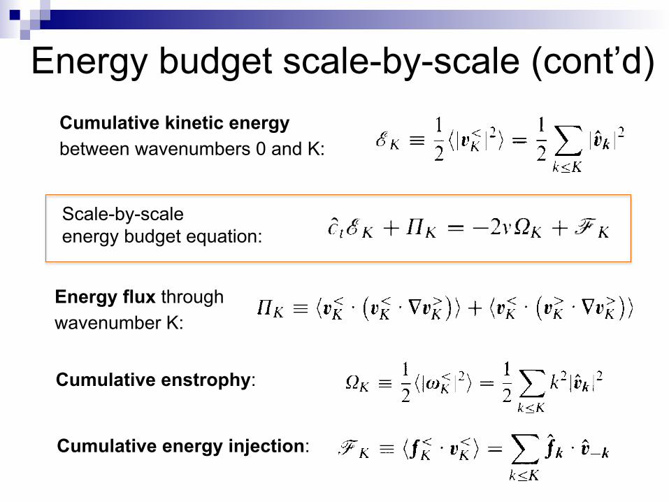
Energy budget scale-by-scale (cont’d) Cumulative kinetic energy between wavenumbers 0 and K:

Scale-by-scale energy budget equation:

Cumulative enstrophy:

Cumulative energy injection:

Energy flux through wavenumber K:

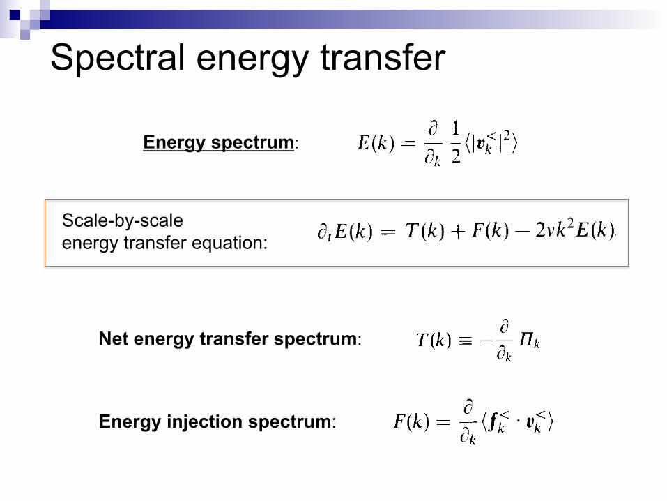
Scale-by-scale energy transfer equation:

Energy spectrum:

Energy injection spectrum:

Net energy transfer spectrum:

Spectral energy transfer

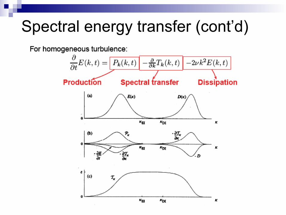
Spectral energy transfer (cont’d)

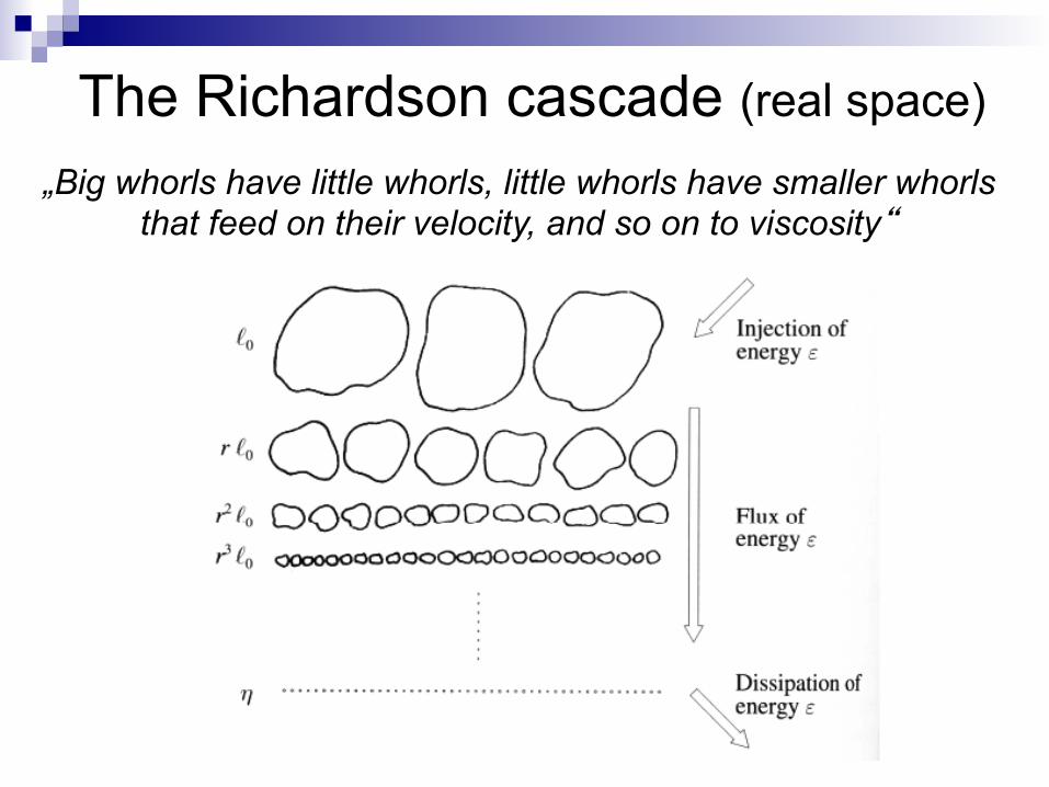
The Richardson cascade (real space)

„Big whorls have little whorls, little whorls have smaller whorls that feed on their velocity, and so on to viscosity“

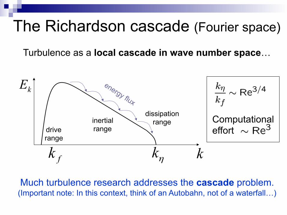
Turbulence as a local cascade in wave number space…

Much turbulence research addresses the cascade problem. (Important note: In this context, think of an Autobahn, not of a waterfall…)

The Richardson cascade (Fourier space)

kE

ηk kfkdrive range

dissipation range inertial

range Computational effort

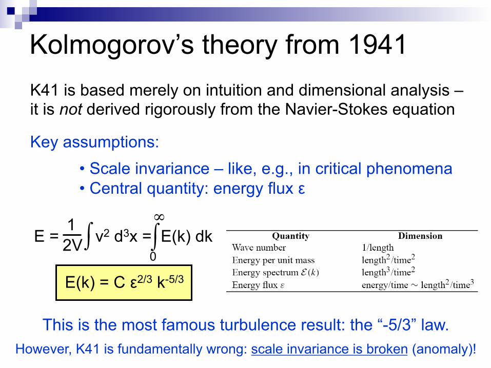
E = v2 d3x = E(k) dk ⌠ ⌡

∞ 1 2V

⌠ ⌡ 0

Kolmogorov’s theory from 1941 K41 is based merely on intuition and dimensional analysis – it is not derived rigorously from the Navier-Stokes equation

Key assumptions:

•  Scale invariance – like, e.g., in critical phenomena •  Central quantity: energy flux ε

E(k) = C ε2/3 k-5/3

This is the most famous turbulence result: the “-5/3” law.

However, K41 is fundamentally wrong: scale invariance is broken (anomaly)!

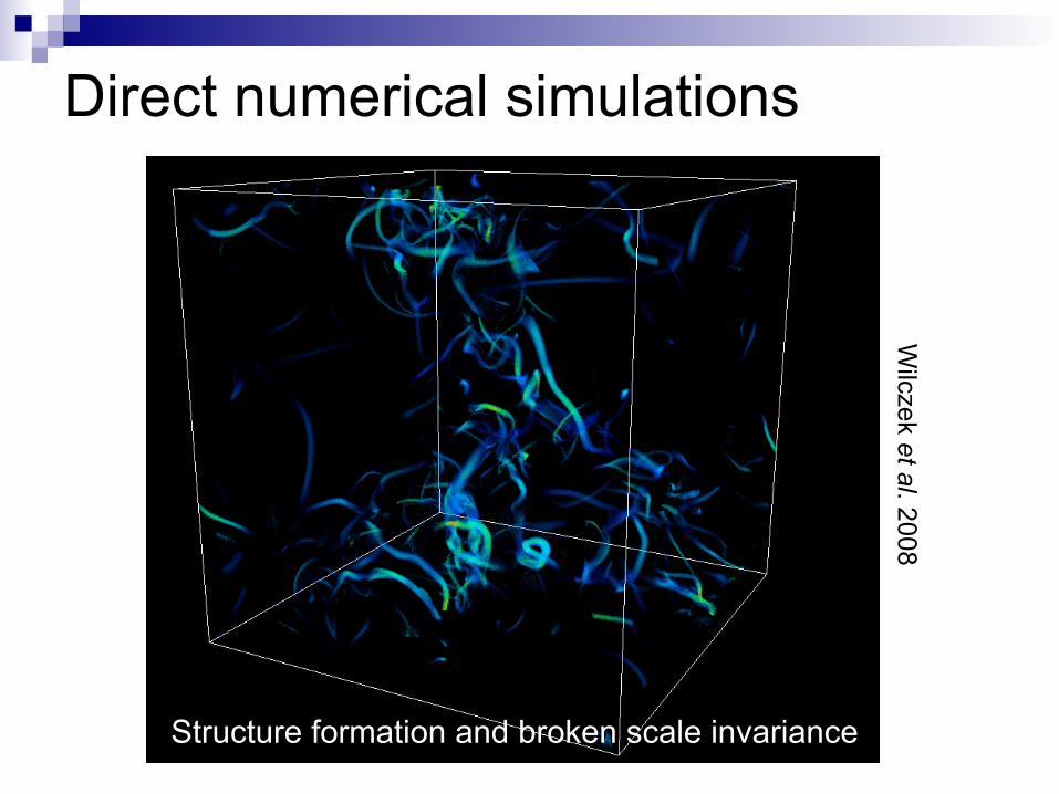
Direct numerical simulations W

ilczek et al. 2008

Structure formation and broken scale invariance

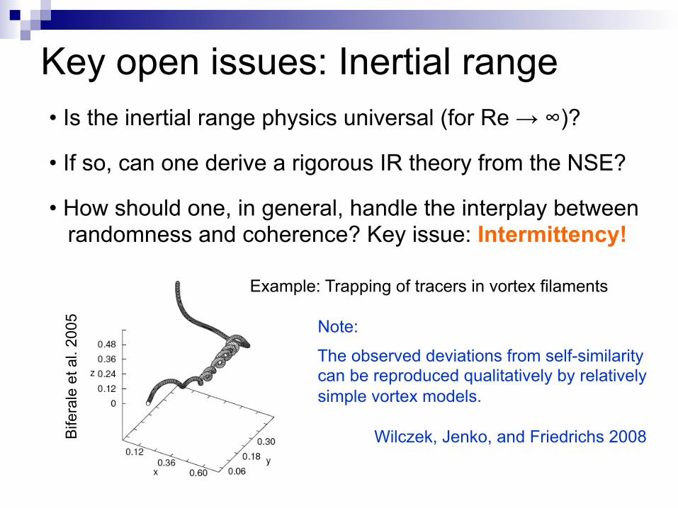
Key open issues: Inertial range •  Is the inertial range physics universal (for Re → ∞)?

•  If so, can one derive a rigorous IR theory from the NSE?

•  How should one, in general, handle the interplay between randomness and coherence? Key issue: Intermittency!

Example: Trapping of tracers in vortex filaments

Note:

The observed deviations from self-similarity can be reproduced qualitatively by relatively simple vortex models.

Wilczek, Jenko, and Friedrichs 2008 B

ifera

le e

t al.

2005

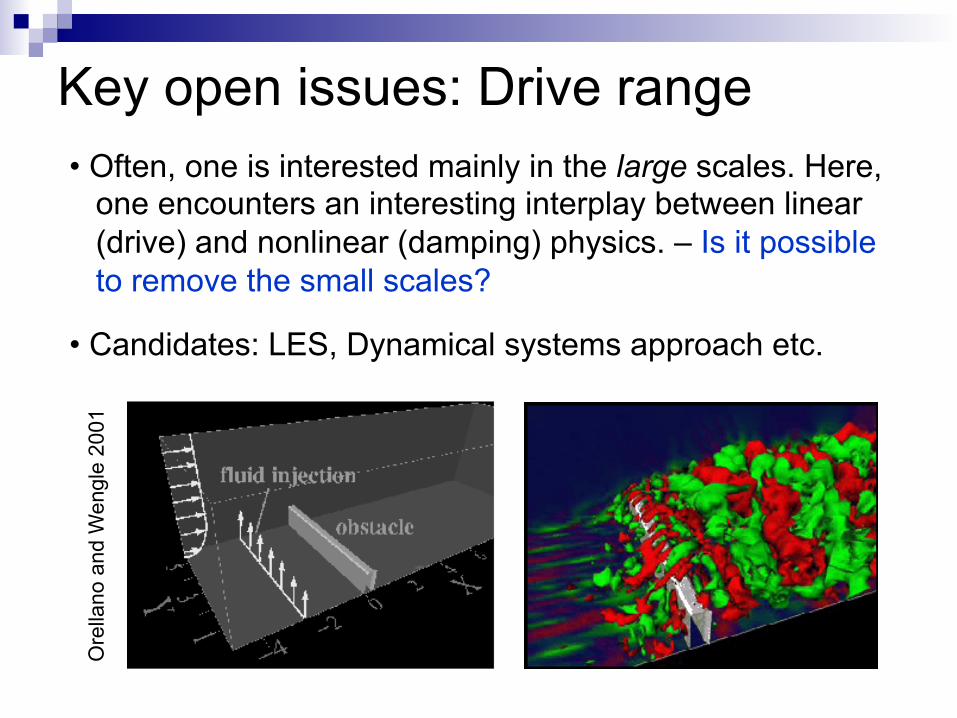
Key open issues: Drive range •  Often, one is interested mainly in the large scales. Here, one encounters an interesting interplay between linear (drive) and nonlinear (damping) physics. – Is it possible to remove the small scales?

•  Candidates: LES, Dynamical systems approach etc.

Ore

llano

and

Wen

gle

2001

On the physics of 2D fluid turbulence

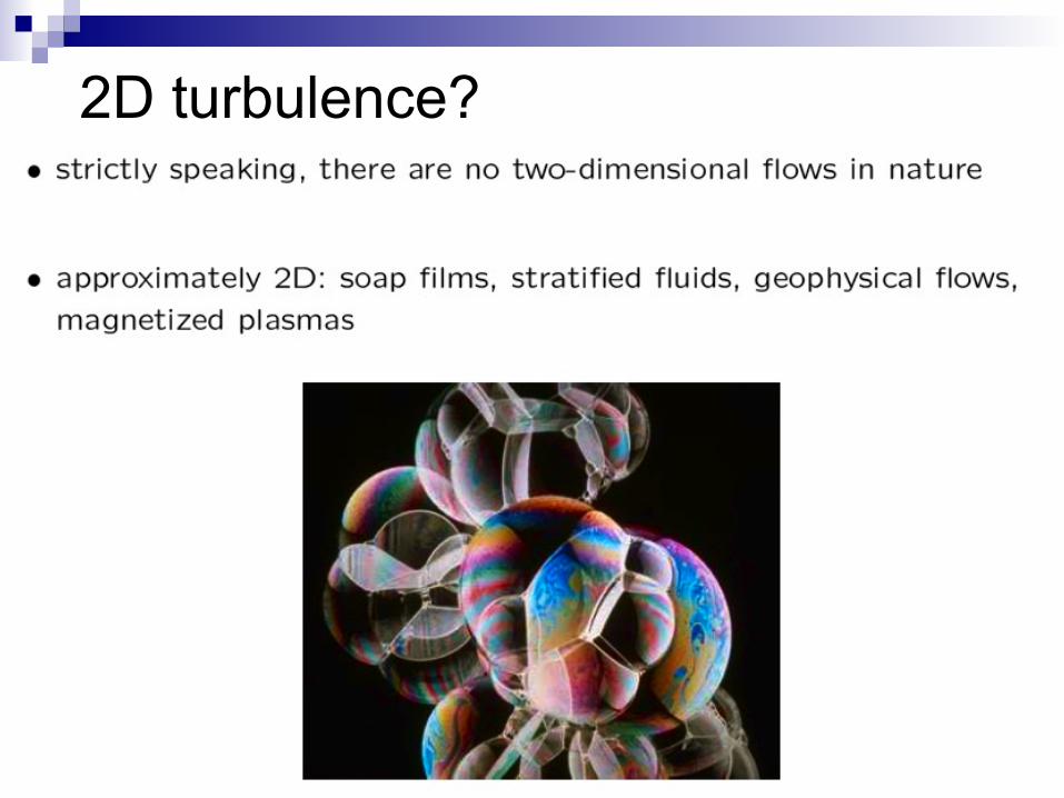
2D turbulence?

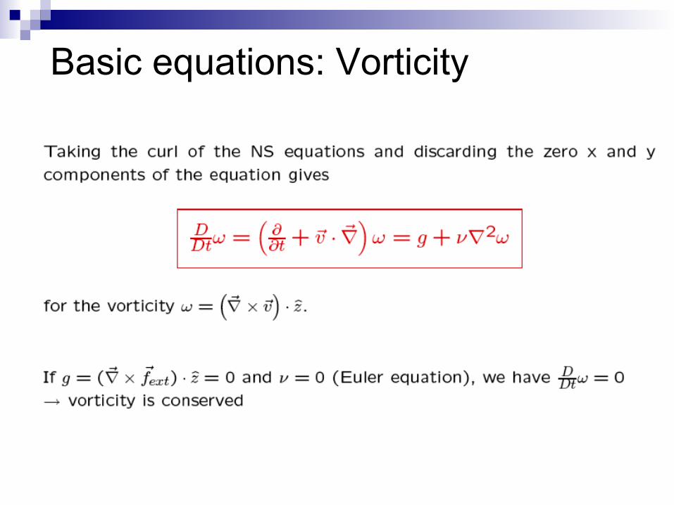
Basic equations: Vorticity

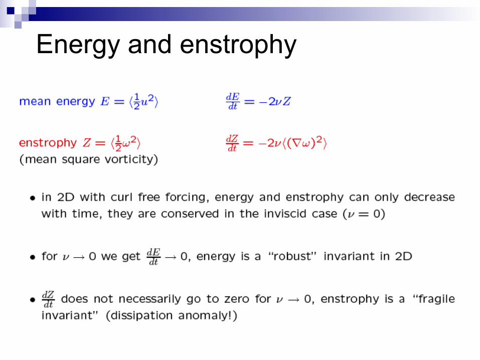
Energy and enstrophy

Cascades

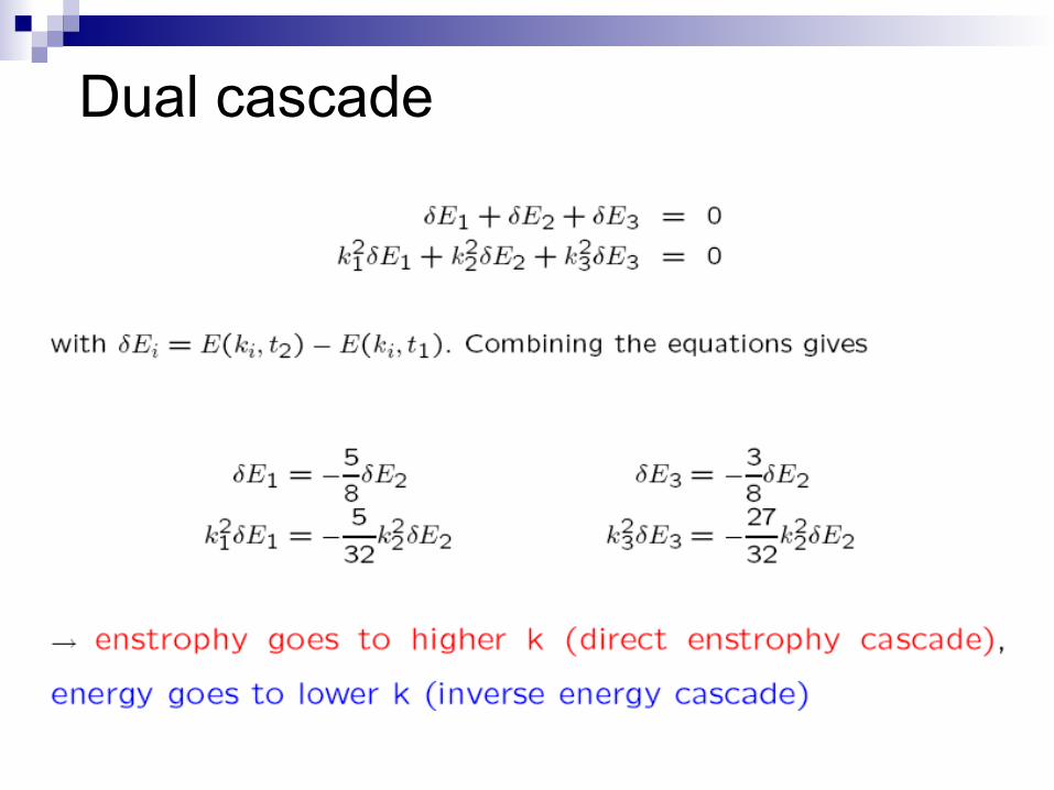
Dual cascade

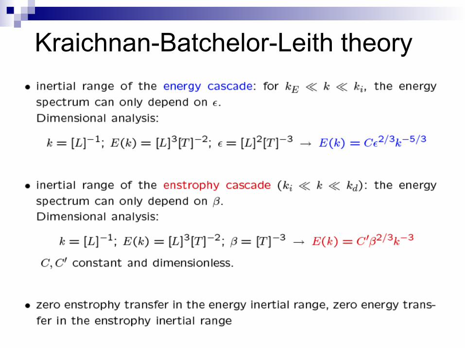
Kraichnan-Batchelor-Leith theory

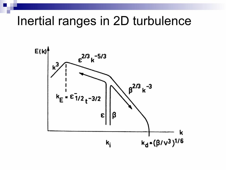
Inertial ranges in 2D turbulence

Turbulence: Further reading

Some literature on 3D turbulence

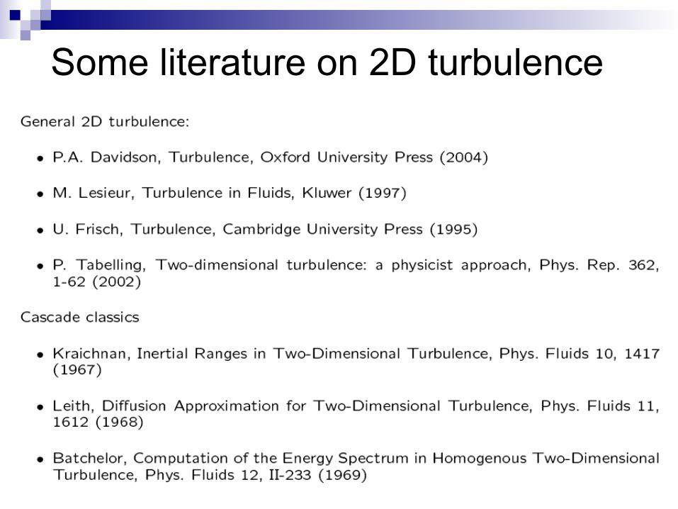
Some literature on 2D turbulence