361-06: 2D Transformations - Computing Science - … Transformations CMPT 361 Introduction to...

© Machiraju/Zhang/Möller

2D Transformations

CMPT 361Introduction to Computer Graphics

Torsten Möller

© Machiraju/Zhang/Möller2

Graphics Pipeline

Hardware

Modelling Transform Visibility

Illumination +Shading

ColorPerception,Interaction

Texture/Realism


Reading• Chapter 3 of Angel• Chapter 5 of Foley, van Dam, …


Schedule• Geometry basics• Affine transformations• Use of homogeneous coordinates• Concatenation of transformations• 3D transformations• Transformation of coordinate systems• Transform the transforms• Transformations in OpenGL


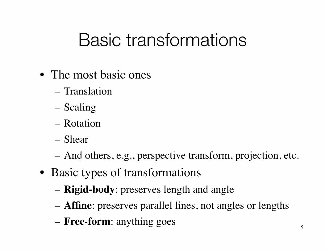
Basic transformations• The most basic ones

– Translation– Scaling– Rotation– Shear– And others, e.g., perspective transform, projection, etc.

• Basic types of transformations– Rigid-body: preserves length and angle– Affine: preserves parallel lines, not angles or lengths– Free-form: anything goes


Translation in 2D

P � = P + T

x� = x + dx

y� = y + dy

�x�

y�

⇥=

�xy

⇥+

�dx

dy

⇥


Scaling in 2D

�x�

y�

⇥=

�sx 00 sy

⇥�

�xy

⇥

P � = S � P

x� = sx � x

y� = sy � y• Uniform sx = sy

• Non-uniform sx ⇥= sy


• Positive angles:counterclockwise

• For negative angles

8

Rotation about origin

P � = R� Px� = x cos(�)� y sin(�)y� = x sin(�) + y cos(�)

cos(��) = cos(�)sin(��) = � sin(�)

�x�

y�

⇥=

�cos(�) � sin(�)sin(�) cos(�)

⇥ �xy

⇥


• Make use of polar coordinates:

9

Derivation of rotation matrix

x = r cos(�)y = r sin(�)

x = r cos(⇥ + �)y = r sin(⇥ + �)

x� = r cos(⇥ + �)= r cos(⇥) cos(�)� r sin(⇥) sin(�)= x cos(�)� y sin(�)

y� = r sin(⇥ + �)= r sin(⇥) cos(�) + r cos(⇥) sin(�)= y cos(�) + x sin(�)

(r, �)� (x, y)

(r, �)� (x, y)


Shearing in 2D

P � = SHy � P

P � = SHx � P�

x�

y�

⇥=

�1 a0 1

⇥ �xy

⇥

�x�

y�

⇥=

�1 0b 1

⇥ �xy

⇥

x� = x + ay

y� = y


Homogeneous coordinates• Only translation cannot be expressed as

matrix-vector multiplications• But we can add a third coordinate –

Homogeneous coordinates for 2D points– (x, y) turns into (x, y, W)– if (x, y, W) and (x', y', W’ ) are multiples of one

another, they represent the same point– typically, W ≠ 0. – points with W = 0 are points at infinity


2D Homogeneous Coordinates• Cartesian coordinates of the homogenous point

(x, y, W): x/W, y/W (divide through by W)• Our typical homogenized points: (x, y, 1) • Connection to 3D?

– (x, y, 1) represents a 3Dpoint on the plane W = 1

– A homogeneous point is aline in 3D, through the origin


Transformation in homogeneous coordinates

• General form of affine (linear) transformation

• E.g., 2D translation in homogeneous coordinates


• 2D line equation– Duality of 3D points to a line

• 3D plane equation:– Duality of 4D points to a plane

• Homog. Coords in 1D?

15

Homogeneous Coords (3)

ax + by + cx + d = 0

�a b c d

⇥

⇤

⌥⌥⇧

xyz1

⌅

��⌃ = 0

ax + by + c = 0

�a b c

⇥⇤

⇧xy1

⌅

⌃ = 0


Basic 2D transformations


Inverse of transformations• Inverse of T(dx, dy) = T(−dx, −dy)

• R(θ)−1 = R(−θ)

• S(sx, sy)−1 = S(1/sx, 1/sy)

• Sh(ax)−1 = Sh(−ax)

T(−dx, −dy) = T(dx, dy)−1


Compound transformations• Often we need many transforms to build

objects (or to “direct” them)– e.g., rotation about an arbitrary point/line?

• Concatenate basic transforms sequentially• This corresponds to multiplication of the

transform matrices, thanks to homogeneous coordinates


Compound translation• What happens when a point goes through

T(dx1, dy1) and then T(dx2, dy2)?

• Combined translation: T(dx1+dx2, dy1+dy2)

Concatenation of transformations: matrix multiplication

�

⇤1 0 dx2

0 1 dy2

0 0 1

⇥

⌅

�

⇤1 0 dx1

0 1 dy1

0 0 1

⇥

⌅ =

�

⇤1 0 dx1 + dx2

0 1 dy1 + dy2

0 0 1

⇥

⌅


Compound rotation• What happens when a point goes through

R(θ) and then R(φ)?• Combined rotation: R(θ + φ)

• Scaling or shearing (in one direction) is similar• These concatenations are commutative


Commutativity• Transformations that do commute:

– Translate – translate– Rotate – rotate (around the same axis)– Scale – scale– Uniform scale – rotate– Shear in x (y) – shear in x (y), etc.

• In general, the order in which transformations are composed is important

• After all, matrix multiplications are not commutative


Commutativity• the order in which we compose matrices is

important: matrix multiplication does not commute

x

y

z

x

y

z x

y

z

x

y

z x

y

z

X then Z

Z then X


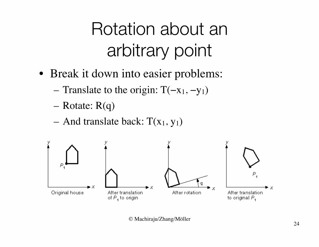
Rotation about an arbitrary point

• Break it down into easier problems:– Translate to the origin: T(−x1, −y1)– Rotate: R(q)– And translate back: T(x1, y1)


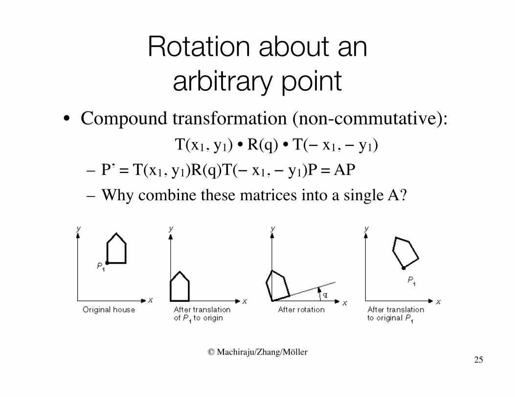
Rotation about an arbitrary point

• Compound transformation (non-commutative):T(x1, y1) • R(q) • T(− x1, − y1)

– P’ = T(x1, y1)R(q)T(− x1, − y1)P = AP– Why combine these matrices into a single A?


Another example• Compound transformation:

T(x2, y2) • R(90o) • S(sx, sy) • T(−x1, −y1)


Rigid-body transformation• A transformation matrix

• where the upper 2 × 2 submatrix is orthonormal, preserves angles and lengths– called rigid-body transformation– any sequence of translation and rotation give a

rigid-body transformation


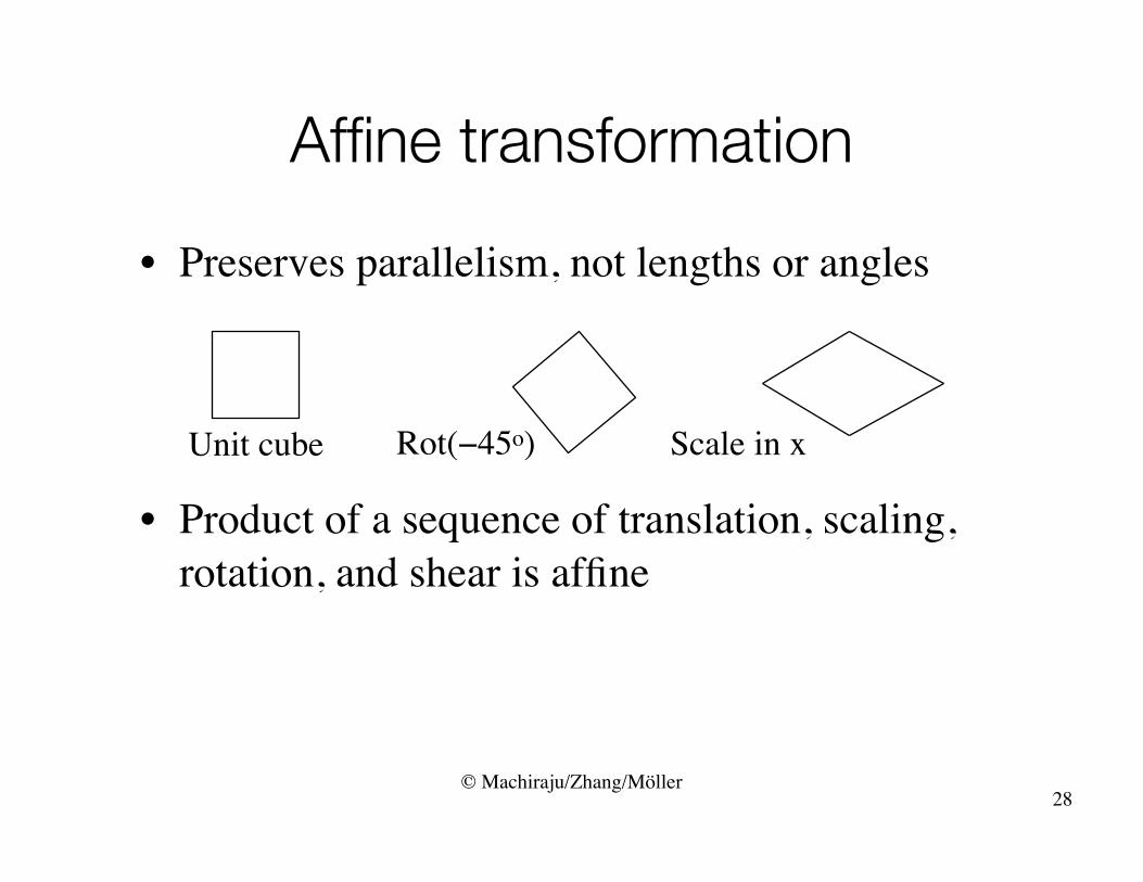
Affine transformation• Preserves parallelism, not lengths or angles

• Product of a sequence of translation, scaling, rotation, and shear is affine

Unit cube Rot(−45o) Scale in x


Types of Transforms• Continuous/Discrete, one to one ; invertible• Classification

– Euclidean (preserves angles)• translation, rotation, uniform scale

– Affine (preserves parallel lines)• Euclidean plus non-uniform scale, shearing

– Projective (preserves lines)– Isometry (preserves distance)

• Reflection, rigid body motion– Nonlinear (lines become curves)

• Twists, Bends, warps, morphs


Window-To-Viewport Transformation

• Important example of compound transform• “World coords”: space users work in• need to map world to the screen

– window in world-coordinate space and– viewport in screen coordinate space


• one can specify non-uniform scaling• results in distorted images• What property of window and viewport

indicates whether the mapping will distort the images?

31

Window-To-Viewport Transformation (2)


Window-To-Viewport Transformation (3)

• Specify transform in matrix form

Mwv = T

�umin

vmin

⇥⇥ S

� umax�uminxmax�xminvmax�vminymax�ymin

⇥⇥ T

��xmin

�ymin

⇥

361-06: 2D Transformations - Computing Science - … Transformations CMPT 361 Introduction to...

Documents

Transcript of 361-06: 2D Transformations - Computing Science - … Transformations CMPT 361 Introduction to...