3410 Electric Power Electromechanical Energy Conversion … · 1 EE – 3410 Electric Power Fall...
30
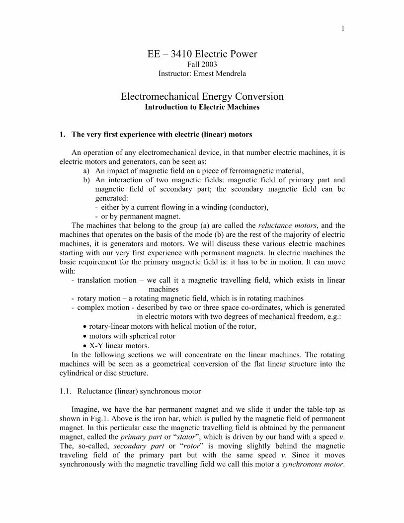
1 EE – 3410 Electric Power Fall 2003 Instructor: Ernest Mendrela Electromechanical Energy Conversion Introduction to Electric Machines 1. The very first experience with electric (linear) motors An operation of any electromechanical device, in that number electric machines, it is electric motors and generators, can be seen as: a) An impact of magnetic field on a piece of ferromagnetic material, b) An interaction of two magnetic fields: magnetic field of primary part and magnetic field of secondary part; the secondary magnetic field can be generated: - either by a current flowing in a winding (conductor), - or by permanent magnet. The machines that belong to the group (a) are called the reluctance motors, and the machines that operates on the basis of the mode (b) are the rest of the majority of electric machines, it is generators and motors. We will discuss these various electric machines starting with our very first experience with permanent magnets. In electric machines the basic requirement for the primary magnetic field is: it has to be in motion. It can move with: - translation motion – we call it a magnetic travelling field, which exists in linear machines - rotary motion – a rotating magnetic field, which is in rotating machines - complex motion - described by two or three space co-ordinates, which is generated in electric motors with two degrees of mechanical freedom, e.g.: • rotary-linear motors with helical motion of the rotor, • motors with spherical rotor • X-Y linear motors. In the following sections we will concentrate on the linear machines. The rotating machines will be seen as a geometrical conversion of the flat linear structure into the cylindrical or disc structure. 1.1. Reluctance (linear) synchronous motor Imagine, we have the bar permanent magnet and we slide it under the table-top as shown in Fig.1. Above is the iron bar, which is pulled by the magnetic field of permanent magnet. In this perticular case the magnetic travelling field is obtained by the permanent magnet, called the primary part or “stator”, which is driven by our hand with a speed v. The, so-called, secondary part or “rotor” is moving slightly behind the magnetic traveling field of the primary part but with the same speed v. Since it moves synchronously with the magnetic travelling field we call this motor a synchronous motor.
-
Upload
trinhkhanh -
Category
Documents
-
view
234 -
download
3
Transcript of 3410 Electric Power Electromechanical Energy Conversion … · 1 EE – 3410 Electric Power Fall...
1
EE ndash 3410 Electric Power Fall 2003
Instructor Ernest Mendrela
Electromechanical Energy Conversion Introduction to Electric Machines
1 The very first experience with electric (linear) motors An operation of any electromechanical device in that number electric machines it is
electric motors and generators can be seen as a) An impact of magnetic field on a piece of ferromagnetic material b) An interaction of two magnetic fields magnetic field of primary part and
magnetic field of secondary part the secondary magnetic field can be generated - either by a current flowing in a winding (conductor) - or by permanent magnet
The machines that belong to the group (a) are called the reluctance motors and the machines that operates on the basis of the mode (b) are the rest of the majority of electric machines it is generators and motors We will discuss these various electric machines starting with our very first experience with permanent magnets In electric machines the basic requirement for the primary magnetic field is it has to be in motion It can move with
- translation motion ndash we call it a magnetic travelling field which exists in linear machines
- rotary motion ndash a rotating magnetic field which is in rotating machines - complex motion - described by two or three space co-ordinates which is generated
in electric motors with two degrees of mechanical freedom eg bull rotary-linear motors with helical motion of the rotor bull motors with spherical rotor bull X-Y linear motors
In the following sections we will concentrate on the linear machines The rotating machines will be seen as a geometrical conversion of the flat linear structure into the cylindrical or disc structure
11 Reluctance (linear) synchronous motor
Imagine we have the bar permanent magnet and we slide it under the table-top as shown in Fig1 Above is the iron bar which is pulled by the magnetic field of permanent magnet In this perticular case the magnetic travelling field is obtained by the permanent magnet called the primary part or ldquostatorrdquo which is driven by our hand with a speed v The so-called secondary part or ldquorotorrdquo is moving slightly behind the magnetic traveling field of the primary part but with the same speed v Since it moves synchronously with the magnetic travelling field we call this motor a synchronous motor
2
The name reluctance means that the reluctance of the magnetic circuit which the magnetic flux is closed through will change as the flux is moving on because of finite length of a secondary part Due to this change the magnetic force is produced that acts on the ldquorotorrdquo If the secondary part would be very (infinitely) long there would be no magnetic force Fx that drive the ldquorotorrdquo There will be only attractive force Fy (see Fig1)
N SN
ldquoRotorrdquo (Fe)
ldquoStatorrdquo (permanent magnet)
Φ (magnetic flux)
S v (speed)
x
Fig1 Linear reluctance motor formed by moving permanent magnet and a piece of solid
iron 12 Permanent magnet (linear) synchronous motor
The secondary part can be in a form of permanent magnet as shown in Fig2 In this case the magnetic force acting on the ldquorotorrdquo is an effect of interaction of two magnetic fields one produced by the ldquostatorrdquo and another one by the ldquorotorrdquo The ldquorotorrdquo moves here synchronously with the magnetic field of the ldquostatorrdquo Because of that and since the secondary part is in form of permanent magnet the motor is called a permanent magnet synchronous motor
N SN
ldquoRotorrdquo (permanent magnet)
ldquoStatorrdquo (permanent magnet)
S v
xNS
Fig2 Linear permanent magnet synchronous motor formed by the moving ldquostatorrdquo
permanent magnet that is pulling the ldquorotorrdquo permanent magnet
So far we analyzed the motors where the primary magnetic field has been produced by the permanent magnet This can be replaced by the electromagnet Its coil may be supplied from the dc voltage source as it is shown in Fig3 The operation of the motor
3
does not differ from the previous motor and to get the magnetic flux moving we must push the electromagnet The motor still can be called permanent magnet linear synchronous motor
ldquorotorrdquo
N S
ldquostatorrdquo
NS NS
vv
coil supplied withdc current
Fig3 Permanent magnet (linear) synchronous motor ldquostatorrdquo magnetic field is produced
by the coil supplied from the dc source 13 Synchronous (linear) motor
The permanent magnet of the secondary part can be replaced by the electromagnet as shown in Fig4 In this case the motor is called synchronous linear motor
i
Fm
1
v
2
g
N
NS
S
ldquostatorrdquo
ldquorotorrdquo
Fig4 Linear synchronous motor ldquostatorrdquo and ldquorotorrdquo are electromagnets The rotating counterpart of the linear motion structure shown in Fig4 is the machine
(in this particular case ndash motor) shown in Fig5 The stator (primary part) electromagnets supplied by the current i1 represent a rotating magnetic field that rotates with angular speed ωm The rotor electromagnet supplied by the current i2 is driven by the torque T slightly behind the stator magnetic field by an angle δ but with the same speed ωm
The magnetic force which acts on the secondary magnet depends on the mutual displacement of both parts If this displacement is expresses in terms of the angle δ as shown in Fig6 then the force Fm changes practically sinusoidally as shown in the graph in Fig7
4
S
N
T
N
Sωm
δ
rotor
stator
i
i 1
2
m
Fig5 Rotary synchronous motor The angle δ is counted from the primary part to the secondary part Therefore it is
negative The maximum negative value the force reaches at angle (-900) The force can be expressed by the function
( )δsinmaxFFm = (1)
or expressed in terms of Cartesianrsquos coordinate
= xFFm τ
πsinmax (2)
where τ is the magnetic pole-pitch (see Fig4)
SN S
ldquostatorrdquo
0
τ(pole pitch)
(x)180 0360 00 minusδ1 δ
S N
ldquorotorrdquo
- F1
0- 180 00
minusδ1δ
0- 90
F (T)
- Fmax(- T )max
Fig6 Linear synchronous motor Fig7 Force (torque) ndash power angle
characteristic of linear (rotary) synchronous motor
In case of cylindrical structure shown in Fig5 the rotor rotates synchronously with the stator magnetic flux due to the torque T acting on the rotor Its value depends sinusoidaly on the angle δ as shown in Fig7
5
2 Force and torque in electric machines
In electric motors the electric energy is converted into mechanical energy In electric generator the process of energy conversion is reversed a mechanical energy is converted into electrical energy In both cases the magnetic field (magnetic flux Φ - see Fig8) is the medium in the electromechanical conversion process
i
Fm
1
v
2
g
ldquostatorrdquo
ldquorotorrdquo
Φ
v1
v2
Fig8 Illustration to electromechanical energy conversion Look at Fig8 In the linear synchronous motor the electric energy is delivered to the
system through the ldquostatorrdquo and ldquorotorrdquo winding terminals called electrical ports This energy is converted to the energy of magnetic field which is next converted into mechanical energy The entire process of energy conversion is shown schematically in Fig9 For the generator the process is reversed the mechanical energy is delivered to the rotor through a rotor shaft and due to the magnetic flux generated by the rotor current it is converted into electrical energy leaving the system through the stator winding terminals (Fig10)
i 1
Stator and rotor windings
Machine magnetic circuit
Machine mechanical system Magnetic flux Magnetic flux Rotor shaft
ωT
i2
e1
WmWfWf
e2
W2e
W1e
Motor
Generator
m
Fig9 Diagram of electromechanical energy conversion no power losses are included During the process of energy conversion the power losses dissipate in the system In
the rotor and stator windings a part of electrical energy is converted into heat due to Ohmic power losses in the winding resistance In the rotor and stator cores part of field energy is lost In the mechanical part of the system part of mechanical energy is lost as
6
heat in bearings and due to the friction between the rotating rotor and the air (windage losses) The process of energy conversion with inclusion of power losses is shown in Fig11 These power losses are converted into the heat energy
S
N T
N
Sωm
δ i
i1
2
v1v2Φ
Fig10 Illustration to electromechanical energy conversion in rotary synchronous generator
i 1
Stator and rotor windings
Machine magnetic circuit
Machine mechanical system Magnetic flux Magnetic flux Rotor shaft
Winding losses
Core losses Mechanical losses
i2
WmWfWf
2
W2e
W1e
R2
e2
W2v
e1W1v
Winding losses
ωT m
R
v
1
1
v
Fig11 Diagram of electromechanical energy conversion with inclusion of power losses
21 Field energy In both motor and generator the field energy is converted either into electric or
mechanical energy In permanent magnet machine the magnetic flux is generated by the magnet and in case of electromagnet the magnetic field is generated by the current
To determine the magnetic field energy stored in the motor let us consider the electromagnetic structure shown in Fig12 consisting of primary part which does not move and the secondary part that can move and which does not have the winding Let assume that at present the secondary part does not move Suppose we increase now the
7
current in the primary winding from 0 to i1 The magnetic flux will rise from 0 to Φ1 as shown in Fig13 We can express the magnetic flux as the flux linkage Φsdot= Nλ which is the product of a number of winding turns and the magnetic flux In case of the real magnetic circuit the λ-i curve is not linear due to the saturation of the iron core For the linear magnetic circuit the λ-i characteristic is a straight line as shown in Fig13b This straight line is described by the equation
iL sdot=λ (3)
where L is a current i coefficient known as winding inductance If we differentiate both sides of the above equation assuming L = const we will obtain the equation for the voltage e induced in the winding
dtdiL
dtde ==λ (4)
i R
v e
g
Fm
Secondarypart (movable)
Primarypart (stationary)
Φ
e
iR1 1
11 v
22
22
Fig12 Illustration to derivation of formula for field energy (a) (b)
λ
ii
N Φ
1
1
λ
L = slope
i
Fig13 Magnetic linkage-current characteristic for (a) ndash nonlinear system (b) ndash for linear system
8
The electric power is equal
edip e i L idt
= sdot = (5)
Since the relation between the power and energy is
ee
dW pdt
= (6)
The increment of electric energy
e edW p dt e i dt L i di= sdot = sdot sdot = sdot sdot (7) In this particular case this energy is a part of the total electric energy delivered to the
winding (see Fig11)
v vdW p dt= sdot (8) where
2
vp v i R i e i= sdot = sdot + sdot (9) Thus We is equal to the magnetic field energy stored in the magnetic flux
fe WW = (10) If the power losses in all elements of the system are ignored and the secondary part is
moving then during the differential time interval dt the increment of electrical energy dWe is equal to the sum
e f mdW dW dW= + (11)
where dWm is the increment of mechanical energy equal to mechanical work done during the time dt by the moving secondary part
If the losses cannot be neglected they can be dealt with separately They do not contribute to the energy conversion process
When the flux linkage is increased from zero to λ1 by means of increase of current from 0 to i1 the energy stored in the field is (Fig14)
1
0fW i d
λ
λ= int (12)
9
λ
fdW
i
λ1
fW
0 Fig14 Field energy on λ-i characteristic
Suppose the air gap of the system in Fig12 increases The λ-i characteristic will
become more flat and straight (see Fig15) To maintain the same magnetic flux (flux linkage) greater current should flow in the winding and consequently greater energy is stored in the magnetic circuit (Fig16) Since the volume of magnetic core remained unchanged the increase of field energy occurred in the air-gap
λ
air-gapincrease
i0
λ
i
gg
λ
1
21
0 i1 i2
Wf1
Wf2
Fig15 λ-I characteristics for various air-gaps in the machine
Fig16 Field energy in the machine with different air-gap
The energy stored in the field can be expressed in terms of other quantities eg
magnetic flux density B in the air gap g To find flux density B for a given current i in the winding we will use the equivalent magnetic circuit of the system shown in Fig17 This circuit does not differ from electric circuit for a dc current and the analogy between the electric and magnetic quantities are shown in Table 1
Table 1
Electric circuit Magnetic circuit Electromofive force (emf) E [V] Current I [A]
Magnetomotive (mmf) Fm = ImiddotN [Amiddotturns] Magnetic flux Φ [Wb]
10
Resistance of conductor w
w
lRA γ
= [Ω]
where lw ndash length of wire [m] Aw ndash cross-section area of the
wire [m2] γ ndash conductivity []
Ohmrsquos law EiR
=
Magnetic resistance (reluctance) of magnetic circuit
mm
m
lRA micro
= [1H] (13)
where lm ndash length of magnetic circuit [m] Am ndash cross-section area of magnetic
circuit [m2] micro ndash magnetic permeability [Hm]
Ohmrsquos law m
m
FR
Φ = (14)
Φm
Fm
Rg
R cHcl c
Hg lg
Magnetic flux Φ is a product
mB AΦ = sdot (15)
of B [T] ndash magnetic flux density and Am [m2] For the linear magnetic circuit a flux density is equal
B H micro= sdot (16)
where H [Am] ndash is the magnetic field intensity in the magnetic circuit
The Ohmrsquos law for magnetic circuit written in other form is
m mF R= Φ sdot (17) Inserting (13) (15) and (16) into (17) we obtain
Fig17 Equivalent magnetic circuit of the electromagnetic system shown in Fig12
11
mm
m
m
m
lI N B AA
lH
H l
micro
micromicro
sdot = sdot
= sdot
= sdot
(18)
where Hlm ndash is the magnetic voltage drop across reluctance of the magnetic circuit
Consider now the electromagnetic system shown in Fig12 with its magnetic equivalent circuit in Fig17 Let
Hc - magnetic intensity in the core Hg - magnetic intensity in the air gap lc ndash total length of the magnetic core lg ndash length of the air-gaps Then
1 c c g gN i H l H lsdot = + (19) The flux linkage
mN N A Bλ = sdotΦ = sdot sdot (20) From Eqs12 19 and 20
c c g gf m
H l H lW N A dl
N+
= sdot sdotint (21)
For the air-gap
0g
BHmicro
= (22)
where micro0 ndash is the magnetic permeability of the vacuum (air-gap) equal to 74 10π minus [Hm]
From Eqs21 and 22
0
0
2
02
f c c g m
c m c m g
c c g
fc c fg g
fc fg
BW H l l A dB
BH dB A l dB A l
BH dB V V
w V w V
W W
micro
micro
micro
= + sdot
= sdot sdot + sdot sdot
= sdot + sdot
= sdot + sdot
= +
int
int
int (23)
12
where
fc cw H dB= int - is the energy density in the magnetic core 2
02fgBwmicro
= - is the energy density in the air-gap
Vc ndash is the volume of the magnetic core Vg ndash is the volume of the air-gap Wfc ndash is the energy in the magnetic core Wfg ndash is the energy in the air-gap
For a linear magnetic core
cc
c
BHmicro
= (24)
therefore
2
2
cfc c c
c
cc
c
BW dB V
B V
micro
micro
= sdot
= sdot
int (25)
Looking at Eqs 23 and 25 we see that the field energy is inversely proportional to the
permeability micro and straight proportional to the volume V If we have the electromechanical system shown in Fig12 in which the same flux density is in both iron cores and air-gap (the same flux Φ and the same cross-section area are for both parts) the magnetic energy is stored mainly in the air-gap since the core permeability is equal to
c o rmicro micro micro= and the relative permeability for unsaturated iron is 1000rmicro gt
22 Co-energy
To calculate the attractive magnetic force acting on the movable part we will
introduce the quantity called co-energy It is defined as
1
0
i
fW diλ= sdotint (26)
It does not have any physical significance Co-energy and energy of the system is shown in Fig18 From Fig18
f fW W iλ+ = sdot (27)
13
If λ-i characteristic is nonlinear f fW Wgt (Fig19 ndash curve g1) but if λ-i characteristic
is linear (straight line g2) f fW W= If the air-gap increases from g1 to g2 and the current
remains unchanged the co-energy will decrease as shown in Fig19
i0
fW
fW lsquo
λ1
λ
i 1
λ
i
ggλ 1
21
0 i1
Wrsquof1
Wrsquof2
λ 2
Fig18 Field energy Wf and field co-energy Wfrsquo
Fig19 Field co-energy for two different values of air-gap in the system
23 Mechanical energy and forces Let us consider the system in Fig20 Let the secondary part moves from one position
(x = x1) to another position (x = x2) The λ-i characteristics of the system for these two positions are shown in Fig21 If the secondary part has moved slowly the current equal to i v R= remains the same at both positions in the steady state because the coil resistance does not change and the voltage is set to be constant
i R
v e
g
Fm
Secondarypart (movable)
Primarypart (stationary)
Φ
e
iR1 1
11 v
22
22
x1x2 0x Fig20 Electromechanical system with movable and stationary parts
14
λ
i
xx
b
ad
c
λ
λ1
2
1
2
0 i1
dWe
Fig21 Illustration to the magnetic force derivation The operation point has moved upward from point a rarr b During the motion
2
1
( )edW e i dt i d area abcdλ
λ
λ= sdot sdot = sdot =int int (28)
the increment of electric energy has been sent to the system The field energy has changed by the increment
(0 0 )fdW area bc ad= minus (29) The mechanical energy
( ) (0 ) (0 )(0 )
m e fdW dW dWarea abcd area ad area bcarea ab
= minus
= + minus=
(30)
is equal to the mechanical work done during the motion of the secondary part and it is represented by the shaded area in Fig21 This shaded area can be seen also as the increase in the co-energy
m fdW dW= (31) Since
m mdW f dx= (32)
the force fm that is causing differential displacement is
( ) fm
i const
W i xf
x=
part=
part (33)
15
231 Force in linear system Let us consider again the system shown in Fig20 The reluctance of the magnetic core path can be ignored due to the high value of microc (see Eq13) and the λ-i characteristic is assumed to be linear The coil inductance L1 depends on the reluctance of the magnetic circuit From Eqs3 and 14 we obtain
m
m
N FLR isdot
= (34)
From Eqs13 and 34 after transformation we obtain
2mN AL
gmicro
= (35)
That means that inductance L depends on length of the air-gap so it is the function of x co-ordinate (see Fig20) Thus for the idealized system
( )L x iλ = (36) where L(x) changes its value with the gap length Since the field co-energy is
0
i
fW diλ= sdotint (37)
after inserting Eq36 for λ we obtain
( )
( )
0
212
i
fW L x i di
L x i
= sdot
=
int (38)
The magnetic force acting on the secondary part we obtain from Eqs33 and 38
( )
( )
2
2
12
12
mi const
f L x ix
dL xi
dx
=
part = part
=
(39)
For a linear system the field energy is equal to the co-energy (Fig19 ndash line g2) thus
16
( ) 212f fW W L x i= = (40)
Force fm can be expressed also in terms of magnetic flux density in the air-gap Bg If we assume that Hc is negligible (due to high permeability microc of the core) then for mechanical system in Fig20 we obtain from Eq19
0
2 2gg
BNi H g g
micro= = (41)
and
0
2gBi g
Nmicro= (42)
From Eqs35 38 and 42 we obtain
2
0
22
gf g
BW A g
micro= sdot sdot (43)
The above expression can be obtained also from the field energy For the linear magnetic circuit
f fW W= therefore from Eq23 (for negligible magnetic energy stored in the core)
2
02
0
2
22
gf g
gg
BW V
BA g
micro
micro
= sdot
= sdot sdot
(44)
where Ag is the cross-section area of the air-gap
From Eqs33 and 43 the force acting on the secondary part is
2
0
2
0
22
22
gm g
gg
Bf A g
g
BA
micro
micro
part= sdot sdot part
= sdot
(45)
It means that the magnetic force is proportional to the magnetic flux density in square
The magnetic pressure Fm that is often used is calculated as the force per unit area of air-gap Thus from Eq45 we have (the cross-section area of the air-gap is 2Ag)
17
2
02g
m
BF
micro= (46)
The expression 45 can be used to calculate the force in all electromechanical devices where the magnetic flux density in the air-gap is known So it can also be applied to determine the driving force in all these primitive linear motors shown in Fgs1 - 4 Let us consider the reluctance linear ldquomotorrdquo shown in Fig22 The magnetic force acting on the ldquorotorrdquo (and the same force but in opposite direction acts on the ldquostatorrdquo) is expressed by Eq45 The driving force fx acting on the ldquorotorrdquo is the tangential (to x axis) component that can be determined from fm if we know the angle β or the mutual displacement ∆x between two motor parts
If we have the reluctance motor with the primary part as an electromagnet (Fig23) we can use formula 39 to determine the linear force fx acting on the secondary part The data that we have to know is the current i flowing in the ldquostatorrdquo winding and the inductance L(x) expressed as the function of x coordinate If the ldquorotorrdquo is infinitely long in x direction as in Fig24 then L = const with respect to x direction and according to Eq23 the force fx = 0 despite very strong attractive force fy acting on the ldquorotorrdquo
N SN
ldquorotorrdquo (Fe)
ldquostatorrdquo
B Sv
x
fmfm
fx
fyy
∆x
δ
Fig22 Force components in linear reluctance motor
i1
vN S
ldquostatorrdquo
ldquorotorrdquo fxx
y
Fig23 Force component Fx produced in the linear reluctance motor The Eqns39 and 45 for force was derived for the system with the coil wound on the primary part only We derive now the force equation for the linear system with the coil wound also on the secondary part (Fig20) as it is in synchronous linear motors shown in Fig8 To do this let us assume again that the secondary part does not move and the field energy is equal to the electric energy
18
1 1 2 2
1 1 2 2
f edW dW e i dt e i dti d i dλ λ
= = +
= + (47)
i1
vN S
ldquostatorrdquo
ldquorotorrdquo
fy
x
y
Fig24 No driving force in the motor with infinitely (very) long ldquorotorrdquo In the linear system (the λ-i characteristic is represented by the straight line see Fig13b) the flux linkages can be expressed in terms of inductances that are constant
1 11 11 12 2
2 21 1 22 2
L i L iL i L i
λλ
= += +
(48)
where L11 ndash is the self inductance of the excitation winding
L22 ndash is the self inductance of the moveable part winding L12 and L21 ndash are the mutual inductances between two windings
From Eqs33 and 34
( ) ( )( )
1 11 1 12 2 2 22 2 21 1
11 1 1 22 2 2 12 1 2
fdW i d L i L i i d L i L i
L i di L i di L d i i
= + + +
= + + (49)
The field energy is equal to the field co-energy for the linear systems Thus we have
( )1 2 1 2
11 1 1 22 2 2 12 1 2
0 0 0
2 211 1 22 2 12 1 2
1 12 2
i i i i
f fW W L i di L i di L d i i
L i L i L i i
= = + +
= + +
int int int (50)
In the system analyzed here the inductances depend on the value of an air-gap It
means that they are functions of position x of secondary part According to Eq33 the force developed by the linear system
19
( )
2 211 22 121 2 1 2
1 12 2
fm
i const
W i xf
x
dL dL dLi i i idx dx dx
=
part=
part
= + +
(51)
The first two terms are the two force components known as reluctance forces The third one is called an electromagnetic force This force exists even if self inductances do not depend on x co-ordinate it is if there are no two first components This type of situation exists in the system shown in Fig25 where either two or one of the part is infinitely (very) long When the secondary moves with respect to the primary self inductances of the coils remain unchanged and only the mutual magnetic coupling (mutual inductance) changes
i1
i2
Fig25 Coils in the infinitely long ldquostatorrdquo and ldquorotorrdquo cores
Equilibrium equations To analyze transients in the windings and dynamic behavior of the motors we have to
write equilibrium equations for electrical ports and mechanical port The equilibrium equations for electrical ports are terminal voltage equations for both primary and secondary windings written on the basis of the second (voltage) Kirhhoffrsquos law applied to equivalent circuit of both windings shown in Fig26 Equation for mechanical port is the equation of motion for mechanical system of the motor shown in Fig27 and written in accordance with the Newtonrsquos Law of Motion The equations written for the electromechanical system shown in Fig20 are as follows
- for electrical ports
11 1 1v R i
tλpart
= +part
(52)
22 2 2v R i
tλpart
= +part
(53)
- for mechanical port
20
2
2m Ld x dxf M D fdt dt
= + + (54)
where
M ndash is mass of the movable part D ndash friction coefficient of the movable secondary part fL ndash load force In the above voltage equations the terminal voltages are equal to the voltage drops
across the winding resistances and the voltages e1 and e2 (see Fig26) induced in the windings by the fluxes linked with them In the motion equation the electromagnetic force developed by the motor is equal to the inertia force friction force and load force
i R
v e e
iR1 1
11 v
22
2
Φ
2
M(x)
v Fig26 Equivalent circuit of the electromechanical system in Fig20
Fm
Secondarypart
D
v
Mmass F - inertiaMF - loadLF - frictionD
Fig27 Equivalent mechanical system of the electromechanical system in Fig20 The derivatives
( )( ) ( )( )
( ) ( ) ( ) ( )
11 1 12 211
11 121 211 1 12 2
L x i L x ie
t t tdL x dL xdi didx dxL x i L x i
dt dx dt dt dx dt
λ part partpart= = +
part part part
= + + +
(55)
21
( )( ) ( )( )
( ) ( ) ( ) ( )
22 2 21 122
22 212 122 2 21 1
L x i L x ie
t t tdL x dL xdi didx dxL x i L x i
dt dx dt dt dx dt
λ part partpart= = +
part part part
= + + +
(56)
Examples of electromechanical devices with a linear (oscillating) motion - transformer with moving coil (for secondary voltage variation) (Fig28)
R1
v1 L11
x
R 1i
2iR2R
L22
M(x)
v2
e 1
e 2
Voltage equations
tiRv
partpart
+= 1111
λ
tiRv
partpart
+= 2222
λ
since 1 11 11 12 2 2 21 1 22 2L i L i and L i L iλ λ= + = + and 11 22 12 21 ( )L L and L L M x= = are constant in
time
( )1 21 1 1 11
di div R i L M xdt dt
= + + or 1 1 1 1v R i e= +
( )2 12 2 2 22
di div R i L M xdt dt
= + + or 2 2 2 2v R i e= +
Fig28 Equivalent circuit of transformer
Changing the distance between the coils we influence M(x) and we change the
voltage e2 and v2 - jumping ring (Fig29)
v
C
Φ
ΦX
X
i1
i2
i1
Fig29 Jumping ring
22
Idea of operation Magnetic flux of the coil Φcoil induces the voltage E2 (and the current i2) in the ring The current i2 in the ring contributes to the flux Φring This flux opposes the flux Φcoil according to phasor diagram in Fig30b (the inductances L11 and E22 are assumed to be much greater than the resistances R1 and R2) As the result the ring is repelled out of the coil
(a) (b)
R1
v1 L1
f em
fg
x
R 1i
2iR2R
L2
M(x)
Aluminum ring
v = 02
C
E1
E2
Φ
V = E
I
E
ΦI
1 1
1
1
2
2
2R2ltlt L2
R1ltlt L1
Fig30 Equivalent circuit of the jumping ring (a) and its phasor diagram (b) When the distance between the coil and ring changes then the resultant inductance of
the coil is changing too If the capacitor C has the value that brings the coil circuit into resonance when the ring is at lowest position then the heavy coil current contributes to the strong force that repels the ring upwards When the ring is far from the coil the resonance disappears consequently the lifting force goes to zero and the ring falls down There the resonance occurs again and the ring is repelled again The resultant effect is the jumping ring The equivalent circuit of the device with jumping ring is shown in Fig30a
- induction linear oscillator (Fig31) The phenomenon described above is applied in induction oscillation motor shown
schematically in Fig31 Two coils are placed at the ends of the ferromagnetic bar Both
vC C
Fig31 Scheme of induction linear oscillator
23
are connected in parallel to the AC source via capacitors If the ring placed between them is close to one of the coil then the resonance occur in the coil and strong repulsion produced force throws the ring to the other coil When the ring appears close to this coil the resonance of this coil will contributes to the repulsion of the ring to the opposite coil Consequently the ring oscillates between the coils
- Reluctance linear oscillator (Fig32)
The ferromagnetic bar loosely placed in the coil is suspended by the attractive
magnetic force produced by the coil magnetic flux (Fig32a) When the bar moves in the coil the coil inductance changes its value If the capacitor connected in series to the coil is chosen to put the circuit into resonance when the bar is at lower position (see Fig32b) then due to the heavy resonance current a strong magnetic force pulls the bar upwards into the coil There the circuit is out of resonance and due to the small current (and no magnetic force at the center of the coil) the bar falls down When it comes at the end of the coil the resonance appears again pulling the bar upwards In consequence the bar will oscillate in vertical position
If the coil is placed in horizontal position as in Fig33 then the resonance current appear at both ends The bar will oscillate in horizontal position To increase the efficiency of the oscillator end-rings are placed at both ends (see Fig34) At the end of the bar track the kinetic energy of the moving bar is not lost but converted into the potential energy of the spring and next returned to the bar This reluctance oscillator is more efficient than the induction oscillator because there are no current losses in the moving part
(a) (b)
R1
v1 L1
f m
f g
xR 1i
D
R1
v1 L1
f m
f g
xR 1i
D
C
x2
1 0
Fig32 Circuit diagrams (a) ferromagnetic bar suspended by the magnetic field (b) electromagnetic device with jumping ferromagnetic bar
24
v
Ci
L(x)i(x)
0
x
x
0xr
Fig33 Scheme of the reluctance linear oscillator with the current and coil inductance characteristics
v
Ci
Fig34 Reluctance linear oscillator with end springs 232 Torque in rotating machines
Let us consider the rotating electromagnetic system shown in Fig35 in which the stator possesses winding 1 and the rotor ndash winding 2 The field co-energy is expressed by Eqn50 The torque developed by the motor is
25
( ) f
i const
W iT
θθ
=
part=
part (57)
From Eqs50 and 57
2 211 22 121 2 1 2
1 12 2
dL dL dLT i i i id d dθ θ θ
= + + (58)
i R
v
iR1 1
1v
22
2em
Rotor
Stator
θ
ω1
e2
Fig35 Rotary motor with salient pole stator and rotor The first two terms are reluctance torques and the third one is an electromagnetic torque For the motor with the round rotor (Fig36) there is no torque represented by the first term since the self inductance of the stator L11 does not depend on the position of the torque (the magnetic flux generated by the first winding does not change as the rotor rotates) Therefore the torque of this motor is described by the following equation
2 22 122 1 2
12
dL dLT i i id dθ θ
= + (59)
i
em
θ
ω
i1
1
2
e2
Fig36 Motor with the salient pole stator and round rotor
Suppose the stator has cylindrical structure and the rotor has salient magnetic poles as shown in Fig37 In such a motor known as synchronous motor with salient poles the
26
self inductance of the rotor winding L22 does not change as the rotor rotates Therefore the torque equation takes the form
2 11 121 1 2
12
dL dLT i i id dθ θ
= + (60)
The first term is the reluctance torque and the second one is known as a synchronous torque
i
m
Rotor
θ
ω
2
i1
Stator
Fig37 Motor with round stator and salient pole rotor Machines with cylindrical stator and rotor A scheme of cylindrical machine is shown in Fig38 The self inductances are constant and therefore no reluctance torque is produced The torque developed by the motor is
121 2
dLT i idθ
= (61)
i
m
θ
ω
2
i1
Fig38 Motor with cylindrical stator and rotor Let the mutual inductance changes sinusoidally
27
12 cosL M θ= (62) where M ndash is the peak value of mutual inductance
θ ndash is the angle between the magnetic axis of the stator and rotor windings
Let the currents in the two windings be
1 1 1cosmi I tω= (63)
( )2 2 2cosmi I tω α= + (64) The position of the rotor with respect to the stator depends on rotor speed and is
mtθ ω δ= + (65) where ωm ndash is the angular velocity of the rotor
δ ndash is the rotor position at t = 0 From Eqns61 62 63 64 and 56 we have
( ) ( )
( )( )( )( )( )( )( )( )
1 2 1 2
1 21 2
1 2
1 2
1 2
cos cos sin
sin4
sin
sin
sin
m m m
m mm
m
m
m
T I I M t t tI I M t
t
t
t
ω ω α ω δ
ω ω ω α δ
ω ω ω α δ
ω ω ω α δ
ω ω ω α δ
= minus + +
= minus + + + +
+ minus + minus + + + minus minus + + minus minus + +
(66)
The torque is the sum of four components which vary sinusoidally with time Therefore the average value of each component is zero unless the coefficients of t are zero Thus the average torque will be nonzero if
( )1 2mω ω ω= plusmn plusmn (67) The machine will develop average torque if it rotates in either direction at a speed that is equal to the sum or difference of the angular frequencies 2 fω π= of the stator and the rotor currents
1 2mω ω ω= plusmn (68) There are two practical cases
1) ω2 = 0 α = 0 ωm = ω1 (single-phase synchronous machine) Rotor carries dc current stator ac current
28
For these conditions from Eqn66
( ) 1 21sin 2 sin
2m mI I MT tω δ δ= minus + + (69)
The instantaneous torque is pulsating It will be constant for poly-phase machine
To find the average torque from Eqn69 we see that average of ( )1sin 2 tω δ+ is zero It means the average torque is
1 2 sin
2avI I MT δ= minus (70)
If ωm = 0 (at starting) the (single-phase) machine does not develop the average
torque
2) ωm = ω1 - ω2 (asynchronous single-phase motor) Both stator and the rotor carry ac currents at different frequencies and rotor speed ωm ne ω1 and ωm ne ω2 From Eq66
( ) ( )( ) ( )
1 21 2
1 2
sin 2 sin 22
sin 2 2 sin
m mI I MT t t
t t
ω α δ ω α δ
ω ω α δ α δ
= minus + + + minus minus +
+ minus minus + + + (71)
The instantaneous torque is pulsating (it is constant in poly-phase motor) The
average value of the torque is
( )1 2 sin4
m mav
I I MT α δ= minus + (72)
At ωm = 0 the average torque is zero A single-phase machine should be brought
to the speed different than 0 so it can produce an average torque This is the principle of operation of induction motor
Equilibrium equations Similar as for linear motor the equilibrium equations for rotating machine are as
follows - for electrical ports voltage equations (the same as Eqns52 and 53)
1
1 1 1v R itλpart
= +part
(73)
29
22 2 2v R i
tλpart
= +part
(74)
The derivatives
( )( ) ( )( )
( ) ( ) ( ) ( )
11 1 12 21
11 121 211 1 12 2
L i L it t t
dL dLdi d di dL i L idt d dt dt d dt
θ θλ
θ θθ θθ θθ θ
part partpart= +
part part part
= + + +
(75)
( )( ) ( )( )
( ) ( ) ( ) ( )
22 2 21 12
22 212 122 2 21 1
L i L it t t
dL dLdi d di dL i L idt d dt dt d dt
θ θλ
θ θθ θθ θθ θ
part partpart= +
part part part
= + + +
(76)
The term mtθ ωpart
=part
is the angular speed of the rotor For the motor considered the
mutual inductances L12 = L21 = M thus
( ) ( ) ( ) ( )111 1 21 11 1 2m m
dL dMdi die L i M it dt d dt d
θ θλ θ ω θ ωθ θ
part= = + + +
part (77)
( ) ( ) ( ) ( )222 2 12 22 2 1m m
dL dMdi die L i M it dt d dt d
θ θλ θ ω θ ωθ θ
part= = + + +
part (78)
The voltages induced in the windings (see Fig36) form two groups The first one
contains the voltages
( ) ( )1 21 11t
di die L Mdt dt
θ θ= + (79)
( ) ( )2 12 22t
di die L Mdt dt
θ θ= + (80)
induced due to the variation in time of the magnetic fluxes represented by the currents that generate them These types of voltages are induced in transformers (index t) The second group
( ) ( )11
1 1 2r m m
dL dMe i i
d dθ θ
ω ωθ θ
= + (81)
( ) ( )22
2 2 1r m m
dL dMe i i
d dθ θ
ω ωθ θ
= + (82)
30
are the voltages induced by the rotation of the rotor In that number the first terms are the voltages induced by the saliency of the rotor and do not exist in the motor with cylindrical stator and the rotor (see Fig38) The second terms are the voltages induced by the mutual rotation of the two windings
- for mechanical port motion equation (Fig39)
2
2 s ld dT J D T Tdt dt
θ θ= + + + (83)
where J ndash moment of inertia of the rotor D ndash friction coefficient of the rotor Tl ndash load torque Ts ndash torsional torque (see Fig40 ndash two torques act in opposite directions and they
twist the shafts by angle ∆θ) which is due to the rotor shaft elasticity and is given by
( )s sT K θ= ∆ (84)
where Ks is the torsional coefficient
Tm
TL
Motor Load
TDTJ
mω
Fig39 Equivalent diagram for mechanical system of the rotary motor Tm ndash
electromagnetic torque TJ ndash inertia torque TD ndash friction torque TL ndash load torque
∆θ
Tm
TL
Motor Load
Fig40 Twist (by the angle ∆θ) of the elastic shaft caused by electromagnetic torque of
the motor Tm and load torque TL acting in oposite direction

2
The name reluctance means that the reluctance of the magnetic circuit which the magnetic flux is closed through will change as the flux is moving on because of finite length of a secondary part Due to this change the magnetic force is produced that acts on the ldquorotorrdquo If the secondary part would be very (infinitely) long there would be no magnetic force Fx that drive the ldquorotorrdquo There will be only attractive force Fy (see Fig1)
N SN
ldquoRotorrdquo (Fe)
ldquoStatorrdquo (permanent magnet)
Φ (magnetic flux)
S v (speed)
x
Fig1 Linear reluctance motor formed by moving permanent magnet and a piece of solid
iron 12 Permanent magnet (linear) synchronous motor
The secondary part can be in a form of permanent magnet as shown in Fig2 In this case the magnetic force acting on the ldquorotorrdquo is an effect of interaction of two magnetic fields one produced by the ldquostatorrdquo and another one by the ldquorotorrdquo The ldquorotorrdquo moves here synchronously with the magnetic field of the ldquostatorrdquo Because of that and since the secondary part is in form of permanent magnet the motor is called a permanent magnet synchronous motor
N SN
ldquoRotorrdquo (permanent magnet)
ldquoStatorrdquo (permanent magnet)
S v
xNS
Fig2 Linear permanent magnet synchronous motor formed by the moving ldquostatorrdquo
permanent magnet that is pulling the ldquorotorrdquo permanent magnet
So far we analyzed the motors where the primary magnetic field has been produced by the permanent magnet This can be replaced by the electromagnet Its coil may be supplied from the dc voltage source as it is shown in Fig3 The operation of the motor
3
does not differ from the previous motor and to get the magnetic flux moving we must push the electromagnet The motor still can be called permanent magnet linear synchronous motor
ldquorotorrdquo
N S
ldquostatorrdquo
NS NS
vv
coil supplied withdc current
Fig3 Permanent magnet (linear) synchronous motor ldquostatorrdquo magnetic field is produced
by the coil supplied from the dc source 13 Synchronous (linear) motor
The permanent magnet of the secondary part can be replaced by the electromagnet as shown in Fig4 In this case the motor is called synchronous linear motor
i
Fm
1
v
2
g
N
NS
S
ldquostatorrdquo
ldquorotorrdquo
Fig4 Linear synchronous motor ldquostatorrdquo and ldquorotorrdquo are electromagnets The rotating counterpart of the linear motion structure shown in Fig4 is the machine
(in this particular case ndash motor) shown in Fig5 The stator (primary part) electromagnets supplied by the current i1 represent a rotating magnetic field that rotates with angular speed ωm The rotor electromagnet supplied by the current i2 is driven by the torque T slightly behind the stator magnetic field by an angle δ but with the same speed ωm
The magnetic force which acts on the secondary magnet depends on the mutual displacement of both parts If this displacement is expresses in terms of the angle δ as shown in Fig6 then the force Fm changes practically sinusoidally as shown in the graph in Fig7
4
S
N
T
N
Sωm
δ
rotor
stator
i
i 1
2
m
Fig5 Rotary synchronous motor The angle δ is counted from the primary part to the secondary part Therefore it is
negative The maximum negative value the force reaches at angle (-900) The force can be expressed by the function
( )δsinmaxFFm = (1)
or expressed in terms of Cartesianrsquos coordinate
= xFFm τ
πsinmax (2)
where τ is the magnetic pole-pitch (see Fig4)
SN S
ldquostatorrdquo
0
τ(pole pitch)
(x)180 0360 00 minusδ1 δ
S N
ldquorotorrdquo
- F1
0- 180 00
minusδ1δ
0- 90
F (T)
- Fmax(- T )max
Fig6 Linear synchronous motor Fig7 Force (torque) ndash power angle
characteristic of linear (rotary) synchronous motor
In case of cylindrical structure shown in Fig5 the rotor rotates synchronously with the stator magnetic flux due to the torque T acting on the rotor Its value depends sinusoidaly on the angle δ as shown in Fig7
5
2 Force and torque in electric machines
In electric motors the electric energy is converted into mechanical energy In electric generator the process of energy conversion is reversed a mechanical energy is converted into electrical energy In both cases the magnetic field (magnetic flux Φ - see Fig8) is the medium in the electromechanical conversion process
i
Fm
1
v
2
g
ldquostatorrdquo
ldquorotorrdquo
Φ
v1
v2
Fig8 Illustration to electromechanical energy conversion Look at Fig8 In the linear synchronous motor the electric energy is delivered to the
system through the ldquostatorrdquo and ldquorotorrdquo winding terminals called electrical ports This energy is converted to the energy of magnetic field which is next converted into mechanical energy The entire process of energy conversion is shown schematically in Fig9 For the generator the process is reversed the mechanical energy is delivered to the rotor through a rotor shaft and due to the magnetic flux generated by the rotor current it is converted into electrical energy leaving the system through the stator winding terminals (Fig10)
i 1
Stator and rotor windings
Machine magnetic circuit
Machine mechanical system Magnetic flux Magnetic flux Rotor shaft
ωT
i2
e1
WmWfWf
e2
W2e
W1e
Motor
Generator
m
Fig9 Diagram of electromechanical energy conversion no power losses are included During the process of energy conversion the power losses dissipate in the system In
the rotor and stator windings a part of electrical energy is converted into heat due to Ohmic power losses in the winding resistance In the rotor and stator cores part of field energy is lost In the mechanical part of the system part of mechanical energy is lost as
6
heat in bearings and due to the friction between the rotating rotor and the air (windage losses) The process of energy conversion with inclusion of power losses is shown in Fig11 These power losses are converted into the heat energy
S
N T
N
Sωm
δ i
i1
2
v1v2Φ
Fig10 Illustration to electromechanical energy conversion in rotary synchronous generator
i 1
Stator and rotor windings
Machine magnetic circuit
Machine mechanical system Magnetic flux Magnetic flux Rotor shaft
Winding losses
Core losses Mechanical losses
i2
WmWfWf
2
W2e
W1e
R2
e2
W2v
e1W1v
Winding losses
ωT m
R
v
1
1
v
Fig11 Diagram of electromechanical energy conversion with inclusion of power losses
21 Field energy In both motor and generator the field energy is converted either into electric or
mechanical energy In permanent magnet machine the magnetic flux is generated by the magnet and in case of electromagnet the magnetic field is generated by the current
To determine the magnetic field energy stored in the motor let us consider the electromagnetic structure shown in Fig12 consisting of primary part which does not move and the secondary part that can move and which does not have the winding Let assume that at present the secondary part does not move Suppose we increase now the
7
current in the primary winding from 0 to i1 The magnetic flux will rise from 0 to Φ1 as shown in Fig13 We can express the magnetic flux as the flux linkage Φsdot= Nλ which is the product of a number of winding turns and the magnetic flux In case of the real magnetic circuit the λ-i curve is not linear due to the saturation of the iron core For the linear magnetic circuit the λ-i characteristic is a straight line as shown in Fig13b This straight line is described by the equation
iL sdot=λ (3)
where L is a current i coefficient known as winding inductance If we differentiate both sides of the above equation assuming L = const we will obtain the equation for the voltage e induced in the winding
dtdiL
dtde ==λ (4)
i R
v e
g
Fm
Secondarypart (movable)
Primarypart (stationary)
Φ
e
iR1 1
11 v
22
22
Fig12 Illustration to derivation of formula for field energy (a) (b)
λ
ii
N Φ
1
1
λ
L = slope
i
Fig13 Magnetic linkage-current characteristic for (a) ndash nonlinear system (b) ndash for linear system
8
The electric power is equal
edip e i L idt
= sdot = (5)
Since the relation between the power and energy is
ee
dW pdt
= (6)
The increment of electric energy
e edW p dt e i dt L i di= sdot = sdot sdot = sdot sdot (7) In this particular case this energy is a part of the total electric energy delivered to the
winding (see Fig11)
v vdW p dt= sdot (8) where
2
vp v i R i e i= sdot = sdot + sdot (9) Thus We is equal to the magnetic field energy stored in the magnetic flux
fe WW = (10) If the power losses in all elements of the system are ignored and the secondary part is
moving then during the differential time interval dt the increment of electrical energy dWe is equal to the sum
e f mdW dW dW= + (11)
where dWm is the increment of mechanical energy equal to mechanical work done during the time dt by the moving secondary part
If the losses cannot be neglected they can be dealt with separately They do not contribute to the energy conversion process
When the flux linkage is increased from zero to λ1 by means of increase of current from 0 to i1 the energy stored in the field is (Fig14)
1
0fW i d
λ
λ= int (12)
9
λ
fdW
i
λ1
fW
0 Fig14 Field energy on λ-i characteristic
Suppose the air gap of the system in Fig12 increases The λ-i characteristic will
become more flat and straight (see Fig15) To maintain the same magnetic flux (flux linkage) greater current should flow in the winding and consequently greater energy is stored in the magnetic circuit (Fig16) Since the volume of magnetic core remained unchanged the increase of field energy occurred in the air-gap
λ
air-gapincrease
i0
λ
i
gg
λ
1
21
0 i1 i2
Wf1
Wf2
Fig15 λ-I characteristics for various air-gaps in the machine
Fig16 Field energy in the machine with different air-gap
The energy stored in the field can be expressed in terms of other quantities eg
magnetic flux density B in the air gap g To find flux density B for a given current i in the winding we will use the equivalent magnetic circuit of the system shown in Fig17 This circuit does not differ from electric circuit for a dc current and the analogy between the electric and magnetic quantities are shown in Table 1
Table 1
Electric circuit Magnetic circuit Electromofive force (emf) E [V] Current I [A]
Magnetomotive (mmf) Fm = ImiddotN [Amiddotturns] Magnetic flux Φ [Wb]
10
Resistance of conductor w
w
lRA γ
= [Ω]
where lw ndash length of wire [m] Aw ndash cross-section area of the
wire [m2] γ ndash conductivity []
Ohmrsquos law EiR
=
Magnetic resistance (reluctance) of magnetic circuit
mm
m
lRA micro
= [1H] (13)
where lm ndash length of magnetic circuit [m] Am ndash cross-section area of magnetic
circuit [m2] micro ndash magnetic permeability [Hm]
Ohmrsquos law m
m
FR
Φ = (14)
Φm
Fm
Rg
R cHcl c
Hg lg
Magnetic flux Φ is a product
mB AΦ = sdot (15)
of B [T] ndash magnetic flux density and Am [m2] For the linear magnetic circuit a flux density is equal
B H micro= sdot (16)
where H [Am] ndash is the magnetic field intensity in the magnetic circuit
The Ohmrsquos law for magnetic circuit written in other form is
m mF R= Φ sdot (17) Inserting (13) (15) and (16) into (17) we obtain
Fig17 Equivalent magnetic circuit of the electromagnetic system shown in Fig12
11
mm
m
m
m
lI N B AA
lH
H l
micro
micromicro
sdot = sdot
= sdot
= sdot
(18)
where Hlm ndash is the magnetic voltage drop across reluctance of the magnetic circuit
Consider now the electromagnetic system shown in Fig12 with its magnetic equivalent circuit in Fig17 Let
Hc - magnetic intensity in the core Hg - magnetic intensity in the air gap lc ndash total length of the magnetic core lg ndash length of the air-gaps Then
1 c c g gN i H l H lsdot = + (19) The flux linkage
mN N A Bλ = sdotΦ = sdot sdot (20) From Eqs12 19 and 20
c c g gf m
H l H lW N A dl
N+
= sdot sdotint (21)
For the air-gap
0g
BHmicro
= (22)
where micro0 ndash is the magnetic permeability of the vacuum (air-gap) equal to 74 10π minus [Hm]
From Eqs21 and 22
0
0
2
02
f c c g m
c m c m g
c c g
fc c fg g
fc fg
BW H l l A dB
BH dB A l dB A l
BH dB V V
w V w V
W W
micro
micro
micro
= + sdot
= sdot sdot + sdot sdot
= sdot + sdot
= sdot + sdot
= +
int
int
int (23)
12
where
fc cw H dB= int - is the energy density in the magnetic core 2
02fgBwmicro
= - is the energy density in the air-gap
Vc ndash is the volume of the magnetic core Vg ndash is the volume of the air-gap Wfc ndash is the energy in the magnetic core Wfg ndash is the energy in the air-gap
For a linear magnetic core
cc
c
BHmicro
= (24)
therefore
2
2
cfc c c
c
cc
c
BW dB V
B V
micro
micro
= sdot
= sdot
int (25)
Looking at Eqs 23 and 25 we see that the field energy is inversely proportional to the
permeability micro and straight proportional to the volume V If we have the electromechanical system shown in Fig12 in which the same flux density is in both iron cores and air-gap (the same flux Φ and the same cross-section area are for both parts) the magnetic energy is stored mainly in the air-gap since the core permeability is equal to
c o rmicro micro micro= and the relative permeability for unsaturated iron is 1000rmicro gt
22 Co-energy
To calculate the attractive magnetic force acting on the movable part we will
introduce the quantity called co-energy It is defined as
1
0
i
fW diλ= sdotint (26)
It does not have any physical significance Co-energy and energy of the system is shown in Fig18 From Fig18
f fW W iλ+ = sdot (27)
13
If λ-i characteristic is nonlinear f fW Wgt (Fig19 ndash curve g1) but if λ-i characteristic
is linear (straight line g2) f fW W= If the air-gap increases from g1 to g2 and the current
remains unchanged the co-energy will decrease as shown in Fig19
i0
fW
fW lsquo
λ1
λ
i 1
λ
i
ggλ 1
21
0 i1
Wrsquof1
Wrsquof2
λ 2
Fig18 Field energy Wf and field co-energy Wfrsquo
Fig19 Field co-energy for two different values of air-gap in the system
23 Mechanical energy and forces Let us consider the system in Fig20 Let the secondary part moves from one position
(x = x1) to another position (x = x2) The λ-i characteristics of the system for these two positions are shown in Fig21 If the secondary part has moved slowly the current equal to i v R= remains the same at both positions in the steady state because the coil resistance does not change and the voltage is set to be constant
i R
v e
g
Fm
Secondarypart (movable)
Primarypart (stationary)
Φ
e
iR1 1
11 v
22
22
x1x2 0x Fig20 Electromechanical system with movable and stationary parts
14
λ
i
xx
b
ad
c
λ
λ1
2
1
2
0 i1
dWe
Fig21 Illustration to the magnetic force derivation The operation point has moved upward from point a rarr b During the motion
2
1
( )edW e i dt i d area abcdλ
λ
λ= sdot sdot = sdot =int int (28)
the increment of electric energy has been sent to the system The field energy has changed by the increment
(0 0 )fdW area bc ad= minus (29) The mechanical energy
( ) (0 ) (0 )(0 )
m e fdW dW dWarea abcd area ad area bcarea ab
= minus
= + minus=
(30)
is equal to the mechanical work done during the motion of the secondary part and it is represented by the shaded area in Fig21 This shaded area can be seen also as the increase in the co-energy
m fdW dW= (31) Since
m mdW f dx= (32)
the force fm that is causing differential displacement is
( ) fm
i const
W i xf
x=
part=
part (33)
15
231 Force in linear system Let us consider again the system shown in Fig20 The reluctance of the magnetic core path can be ignored due to the high value of microc (see Eq13) and the λ-i characteristic is assumed to be linear The coil inductance L1 depends on the reluctance of the magnetic circuit From Eqs3 and 14 we obtain
m
m
N FLR isdot
= (34)
From Eqs13 and 34 after transformation we obtain
2mN AL
gmicro
= (35)
That means that inductance L depends on length of the air-gap so it is the function of x co-ordinate (see Fig20) Thus for the idealized system
( )L x iλ = (36) where L(x) changes its value with the gap length Since the field co-energy is
0
i
fW diλ= sdotint (37)
after inserting Eq36 for λ we obtain
( )
( )
0
212
i
fW L x i di
L x i
= sdot
=
int (38)
The magnetic force acting on the secondary part we obtain from Eqs33 and 38
( )
( )
2
2
12
12
mi const
f L x ix
dL xi
dx
=
part = part
=
(39)
For a linear system the field energy is equal to the co-energy (Fig19 ndash line g2) thus
16
( ) 212f fW W L x i= = (40)
Force fm can be expressed also in terms of magnetic flux density in the air-gap Bg If we assume that Hc is negligible (due to high permeability microc of the core) then for mechanical system in Fig20 we obtain from Eq19
0
2 2gg
BNi H g g
micro= = (41)
and
0
2gBi g
Nmicro= (42)
From Eqs35 38 and 42 we obtain
2
0
22
gf g
BW A g
micro= sdot sdot (43)
The above expression can be obtained also from the field energy For the linear magnetic circuit
f fW W= therefore from Eq23 (for negligible magnetic energy stored in the core)
2
02
0
2
22
gf g
gg
BW V
BA g
micro
micro
= sdot
= sdot sdot
(44)
where Ag is the cross-section area of the air-gap
From Eqs33 and 43 the force acting on the secondary part is
2
0
2
0
22
22
gm g
gg
Bf A g
g
BA
micro
micro
part= sdot sdot part
= sdot
(45)
It means that the magnetic force is proportional to the magnetic flux density in square
The magnetic pressure Fm that is often used is calculated as the force per unit area of air-gap Thus from Eq45 we have (the cross-section area of the air-gap is 2Ag)
17
2
02g
m
BF
micro= (46)
The expression 45 can be used to calculate the force in all electromechanical devices where the magnetic flux density in the air-gap is known So it can also be applied to determine the driving force in all these primitive linear motors shown in Fgs1 - 4 Let us consider the reluctance linear ldquomotorrdquo shown in Fig22 The magnetic force acting on the ldquorotorrdquo (and the same force but in opposite direction acts on the ldquostatorrdquo) is expressed by Eq45 The driving force fx acting on the ldquorotorrdquo is the tangential (to x axis) component that can be determined from fm if we know the angle β or the mutual displacement ∆x between two motor parts
If we have the reluctance motor with the primary part as an electromagnet (Fig23) we can use formula 39 to determine the linear force fx acting on the secondary part The data that we have to know is the current i flowing in the ldquostatorrdquo winding and the inductance L(x) expressed as the function of x coordinate If the ldquorotorrdquo is infinitely long in x direction as in Fig24 then L = const with respect to x direction and according to Eq23 the force fx = 0 despite very strong attractive force fy acting on the ldquorotorrdquo
N SN
ldquorotorrdquo (Fe)
ldquostatorrdquo
B Sv
x
fmfm
fx
fyy
∆x
δ
Fig22 Force components in linear reluctance motor
i1
vN S
ldquostatorrdquo
ldquorotorrdquo fxx
y
Fig23 Force component Fx produced in the linear reluctance motor The Eqns39 and 45 for force was derived for the system with the coil wound on the primary part only We derive now the force equation for the linear system with the coil wound also on the secondary part (Fig20) as it is in synchronous linear motors shown in Fig8 To do this let us assume again that the secondary part does not move and the field energy is equal to the electric energy
18
1 1 2 2
1 1 2 2
f edW dW e i dt e i dti d i dλ λ
= = +
= + (47)
i1
vN S
ldquostatorrdquo
ldquorotorrdquo
fy
x
y
Fig24 No driving force in the motor with infinitely (very) long ldquorotorrdquo In the linear system (the λ-i characteristic is represented by the straight line see Fig13b) the flux linkages can be expressed in terms of inductances that are constant
1 11 11 12 2
2 21 1 22 2
L i L iL i L i
λλ
= += +
(48)
where L11 ndash is the self inductance of the excitation winding
L22 ndash is the self inductance of the moveable part winding L12 and L21 ndash are the mutual inductances between two windings
From Eqs33 and 34
( ) ( )( )
1 11 1 12 2 2 22 2 21 1
11 1 1 22 2 2 12 1 2
fdW i d L i L i i d L i L i
L i di L i di L d i i
= + + +
= + + (49)
The field energy is equal to the field co-energy for the linear systems Thus we have
( )1 2 1 2
11 1 1 22 2 2 12 1 2
0 0 0
2 211 1 22 2 12 1 2
1 12 2
i i i i
f fW W L i di L i di L d i i
L i L i L i i
= = + +
= + +
int int int (50)
In the system analyzed here the inductances depend on the value of an air-gap It
means that they are functions of position x of secondary part According to Eq33 the force developed by the linear system
19
( )
2 211 22 121 2 1 2
1 12 2
fm
i const
W i xf
x
dL dL dLi i i idx dx dx
=
part=
part
= + +
(51)
The first two terms are the two force components known as reluctance forces The third one is called an electromagnetic force This force exists even if self inductances do not depend on x co-ordinate it is if there are no two first components This type of situation exists in the system shown in Fig25 where either two or one of the part is infinitely (very) long When the secondary moves with respect to the primary self inductances of the coils remain unchanged and only the mutual magnetic coupling (mutual inductance) changes
i1
i2
Fig25 Coils in the infinitely long ldquostatorrdquo and ldquorotorrdquo cores
Equilibrium equations To analyze transients in the windings and dynamic behavior of the motors we have to
write equilibrium equations for electrical ports and mechanical port The equilibrium equations for electrical ports are terminal voltage equations for both primary and secondary windings written on the basis of the second (voltage) Kirhhoffrsquos law applied to equivalent circuit of both windings shown in Fig26 Equation for mechanical port is the equation of motion for mechanical system of the motor shown in Fig27 and written in accordance with the Newtonrsquos Law of Motion The equations written for the electromechanical system shown in Fig20 are as follows
- for electrical ports
11 1 1v R i
tλpart
= +part
(52)
22 2 2v R i
tλpart
= +part
(53)
- for mechanical port
20
2
2m Ld x dxf M D fdt dt
= + + (54)
where
M ndash is mass of the movable part D ndash friction coefficient of the movable secondary part fL ndash load force In the above voltage equations the terminal voltages are equal to the voltage drops
across the winding resistances and the voltages e1 and e2 (see Fig26) induced in the windings by the fluxes linked with them In the motion equation the electromagnetic force developed by the motor is equal to the inertia force friction force and load force
i R
v e e
iR1 1
11 v
22
2
Φ
2
M(x)
v Fig26 Equivalent circuit of the electromechanical system in Fig20
Fm
Secondarypart
D
v
Mmass F - inertiaMF - loadLF - frictionD
Fig27 Equivalent mechanical system of the electromechanical system in Fig20 The derivatives
( )( ) ( )( )
( ) ( ) ( ) ( )
11 1 12 211
11 121 211 1 12 2
L x i L x ie
t t tdL x dL xdi didx dxL x i L x i
dt dx dt dt dx dt
λ part partpart= = +
part part part
= + + +
(55)
21
( )( ) ( )( )
( ) ( ) ( ) ( )
22 2 21 122
22 212 122 2 21 1
L x i L x ie
t t tdL x dL xdi didx dxL x i L x i
dt dx dt dt dx dt
λ part partpart= = +
part part part
= + + +
(56)
Examples of electromechanical devices with a linear (oscillating) motion - transformer with moving coil (for secondary voltage variation) (Fig28)
R1
v1 L11
x
R 1i
2iR2R
L22
M(x)
v2
e 1
e 2
Voltage equations
tiRv
partpart
+= 1111
λ
tiRv
partpart
+= 2222
λ
since 1 11 11 12 2 2 21 1 22 2L i L i and L i L iλ λ= + = + and 11 22 12 21 ( )L L and L L M x= = are constant in
time
( )1 21 1 1 11
di div R i L M xdt dt
= + + or 1 1 1 1v R i e= +
( )2 12 2 2 22
di div R i L M xdt dt
= + + or 2 2 2 2v R i e= +
Fig28 Equivalent circuit of transformer
Changing the distance between the coils we influence M(x) and we change the
voltage e2 and v2 - jumping ring (Fig29)
v
C
Φ
ΦX
X
i1
i2
i1
Fig29 Jumping ring
22
Idea of operation Magnetic flux of the coil Φcoil induces the voltage E2 (and the current i2) in the ring The current i2 in the ring contributes to the flux Φring This flux opposes the flux Φcoil according to phasor diagram in Fig30b (the inductances L11 and E22 are assumed to be much greater than the resistances R1 and R2) As the result the ring is repelled out of the coil
(a) (b)
R1
v1 L1
f em
fg
x
R 1i
2iR2R
L2
M(x)
Aluminum ring
v = 02
C
E1
E2
Φ
V = E
I
E
ΦI
1 1
1
1
2
2
2R2ltlt L2
R1ltlt L1
Fig30 Equivalent circuit of the jumping ring (a) and its phasor diagram (b) When the distance between the coil and ring changes then the resultant inductance of
the coil is changing too If the capacitor C has the value that brings the coil circuit into resonance when the ring is at lowest position then the heavy coil current contributes to the strong force that repels the ring upwards When the ring is far from the coil the resonance disappears consequently the lifting force goes to zero and the ring falls down There the resonance occurs again and the ring is repelled again The resultant effect is the jumping ring The equivalent circuit of the device with jumping ring is shown in Fig30a
- induction linear oscillator (Fig31) The phenomenon described above is applied in induction oscillation motor shown
schematically in Fig31 Two coils are placed at the ends of the ferromagnetic bar Both
vC C
Fig31 Scheme of induction linear oscillator
23
are connected in parallel to the AC source via capacitors If the ring placed between them is close to one of the coil then the resonance occur in the coil and strong repulsion produced force throws the ring to the other coil When the ring appears close to this coil the resonance of this coil will contributes to the repulsion of the ring to the opposite coil Consequently the ring oscillates between the coils
- Reluctance linear oscillator (Fig32)
The ferromagnetic bar loosely placed in the coil is suspended by the attractive
magnetic force produced by the coil magnetic flux (Fig32a) When the bar moves in the coil the coil inductance changes its value If the capacitor connected in series to the coil is chosen to put the circuit into resonance when the bar is at lower position (see Fig32b) then due to the heavy resonance current a strong magnetic force pulls the bar upwards into the coil There the circuit is out of resonance and due to the small current (and no magnetic force at the center of the coil) the bar falls down When it comes at the end of the coil the resonance appears again pulling the bar upwards In consequence the bar will oscillate in vertical position
If the coil is placed in horizontal position as in Fig33 then the resonance current appear at both ends The bar will oscillate in horizontal position To increase the efficiency of the oscillator end-rings are placed at both ends (see Fig34) At the end of the bar track the kinetic energy of the moving bar is not lost but converted into the potential energy of the spring and next returned to the bar This reluctance oscillator is more efficient than the induction oscillator because there are no current losses in the moving part
(a) (b)
R1
v1 L1
f m
f g
xR 1i
D
R1
v1 L1
f m
f g
xR 1i
D
C
x2
1 0
Fig32 Circuit diagrams (a) ferromagnetic bar suspended by the magnetic field (b) electromagnetic device with jumping ferromagnetic bar
24
v
Ci
L(x)i(x)
0
x
x
0xr
Fig33 Scheme of the reluctance linear oscillator with the current and coil inductance characteristics
v
Ci
Fig34 Reluctance linear oscillator with end springs 232 Torque in rotating machines
Let us consider the rotating electromagnetic system shown in Fig35 in which the stator possesses winding 1 and the rotor ndash winding 2 The field co-energy is expressed by Eqn50 The torque developed by the motor is
25
( ) f
i const
W iT
θθ
=
part=
part (57)
From Eqs50 and 57
2 211 22 121 2 1 2
1 12 2
dL dL dLT i i i id d dθ θ θ
= + + (58)
i R
v
iR1 1
1v
22
2em
Rotor
Stator
θ
ω1
e2
Fig35 Rotary motor with salient pole stator and rotor The first two terms are reluctance torques and the third one is an electromagnetic torque For the motor with the round rotor (Fig36) there is no torque represented by the first term since the self inductance of the stator L11 does not depend on the position of the torque (the magnetic flux generated by the first winding does not change as the rotor rotates) Therefore the torque of this motor is described by the following equation
2 22 122 1 2
12
dL dLT i i id dθ θ
= + (59)
i
em
θ
ω
i1
1
2
e2
Fig36 Motor with the salient pole stator and round rotor
Suppose the stator has cylindrical structure and the rotor has salient magnetic poles as shown in Fig37 In such a motor known as synchronous motor with salient poles the
26
self inductance of the rotor winding L22 does not change as the rotor rotates Therefore the torque equation takes the form
2 11 121 1 2
12
dL dLT i i id dθ θ
= + (60)
The first term is the reluctance torque and the second one is known as a synchronous torque
i
m
Rotor
θ
ω
2
i1
Stator
Fig37 Motor with round stator and salient pole rotor Machines with cylindrical stator and rotor A scheme of cylindrical machine is shown in Fig38 The self inductances are constant and therefore no reluctance torque is produced The torque developed by the motor is
121 2
dLT i idθ
= (61)
i
m
θ
ω
2
i1
Fig38 Motor with cylindrical stator and rotor Let the mutual inductance changes sinusoidally
27
12 cosL M θ= (62) where M ndash is the peak value of mutual inductance
θ ndash is the angle between the magnetic axis of the stator and rotor windings
Let the currents in the two windings be
1 1 1cosmi I tω= (63)
( )2 2 2cosmi I tω α= + (64) The position of the rotor with respect to the stator depends on rotor speed and is
mtθ ω δ= + (65) where ωm ndash is the angular velocity of the rotor
δ ndash is the rotor position at t = 0 From Eqns61 62 63 64 and 56 we have
( ) ( )
( )( )( )( )( )( )( )( )
1 2 1 2
1 21 2
1 2
1 2
1 2
cos cos sin
sin4
sin
sin
sin
m m m
m mm
m
m
m
T I I M t t tI I M t
t
t
t
ω ω α ω δ
ω ω ω α δ
ω ω ω α δ
ω ω ω α δ
ω ω ω α δ
= minus + +
= minus + + + +
+ minus + minus + + + minus minus + + minus minus + +
(66)
The torque is the sum of four components which vary sinusoidally with time Therefore the average value of each component is zero unless the coefficients of t are zero Thus the average torque will be nonzero if
( )1 2mω ω ω= plusmn plusmn (67) The machine will develop average torque if it rotates in either direction at a speed that is equal to the sum or difference of the angular frequencies 2 fω π= of the stator and the rotor currents
1 2mω ω ω= plusmn (68) There are two practical cases
1) ω2 = 0 α = 0 ωm = ω1 (single-phase synchronous machine) Rotor carries dc current stator ac current
28
For these conditions from Eqn66
( ) 1 21sin 2 sin
2m mI I MT tω δ δ= minus + + (69)
The instantaneous torque is pulsating It will be constant for poly-phase machine
To find the average torque from Eqn69 we see that average of ( )1sin 2 tω δ+ is zero It means the average torque is
1 2 sin
2avI I MT δ= minus (70)
If ωm = 0 (at starting) the (single-phase) machine does not develop the average
torque
2) ωm = ω1 - ω2 (asynchronous single-phase motor) Both stator and the rotor carry ac currents at different frequencies and rotor speed ωm ne ω1 and ωm ne ω2 From Eq66
( ) ( )( ) ( )
1 21 2
1 2
sin 2 sin 22
sin 2 2 sin
m mI I MT t t
t t
ω α δ ω α δ
ω ω α δ α δ
= minus + + + minus minus +
+ minus minus + + + (71)
The instantaneous torque is pulsating (it is constant in poly-phase motor) The
average value of the torque is
( )1 2 sin4
m mav
I I MT α δ= minus + (72)
At ωm = 0 the average torque is zero A single-phase machine should be brought
to the speed different than 0 so it can produce an average torque This is the principle of operation of induction motor
Equilibrium equations Similar as for linear motor the equilibrium equations for rotating machine are as
follows - for electrical ports voltage equations (the same as Eqns52 and 53)
1
1 1 1v R itλpart
= +part
(73)
29
22 2 2v R i
tλpart
= +part
(74)
The derivatives
( )( ) ( )( )
( ) ( ) ( ) ( )
11 1 12 21
11 121 211 1 12 2
L i L it t t
dL dLdi d di dL i L idt d dt dt d dt
θ θλ
θ θθ θθ θθ θ
part partpart= +
part part part
= + + +
(75)
( )( ) ( )( )
( ) ( ) ( ) ( )
22 2 21 12
22 212 122 2 21 1
L i L it t t
dL dLdi d di dL i L idt d dt dt d dt
θ θλ
θ θθ θθ θθ θ
part partpart= +
part part part
= + + +
(76)
The term mtθ ωpart
=part
is the angular speed of the rotor For the motor considered the
mutual inductances L12 = L21 = M thus
( ) ( ) ( ) ( )111 1 21 11 1 2m m
dL dMdi die L i M it dt d dt d
θ θλ θ ω θ ωθ θ
part= = + + +
part (77)
( ) ( ) ( ) ( )222 2 12 22 2 1m m
dL dMdi die L i M it dt d dt d
θ θλ θ ω θ ωθ θ
part= = + + +
part (78)
The voltages induced in the windings (see Fig36) form two groups The first one
contains the voltages
( ) ( )1 21 11t
di die L Mdt dt
θ θ= + (79)
( ) ( )2 12 22t
di die L Mdt dt
θ θ= + (80)
induced due to the variation in time of the magnetic fluxes represented by the currents that generate them These types of voltages are induced in transformers (index t) The second group
( ) ( )11
1 1 2r m m
dL dMe i i
d dθ θ
ω ωθ θ
= + (81)
( ) ( )22
2 2 1r m m
dL dMe i i
d dθ θ
ω ωθ θ
= + (82)
30
are the voltages induced by the rotation of the rotor In that number the first terms are the voltages induced by the saliency of the rotor and do not exist in the motor with cylindrical stator and the rotor (see Fig38) The second terms are the voltages induced by the mutual rotation of the two windings
- for mechanical port motion equation (Fig39)
2
2 s ld dT J D T Tdt dt
θ θ= + + + (83)
where J ndash moment of inertia of the rotor D ndash friction coefficient of the rotor Tl ndash load torque Ts ndash torsional torque (see Fig40 ndash two torques act in opposite directions and they
twist the shafts by angle ∆θ) which is due to the rotor shaft elasticity and is given by
( )s sT K θ= ∆ (84)
where Ks is the torsional coefficient
Tm
TL
Motor Load
TDTJ
mω
Fig39 Equivalent diagram for mechanical system of the rotary motor Tm ndash
electromagnetic torque TJ ndash inertia torque TD ndash friction torque TL ndash load torque
∆θ
Tm
TL
Motor Load
Fig40 Twist (by the angle ∆θ) of the elastic shaft caused by electromagnetic torque of
the motor Tm and load torque TL acting in oposite direction
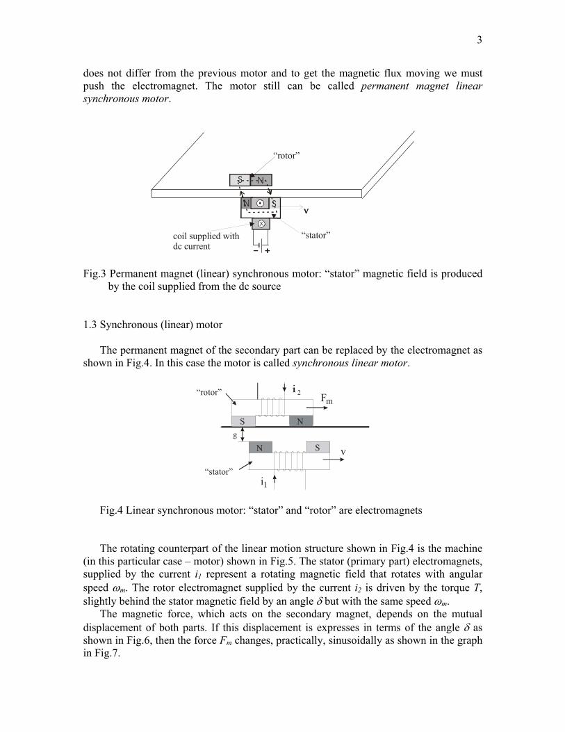
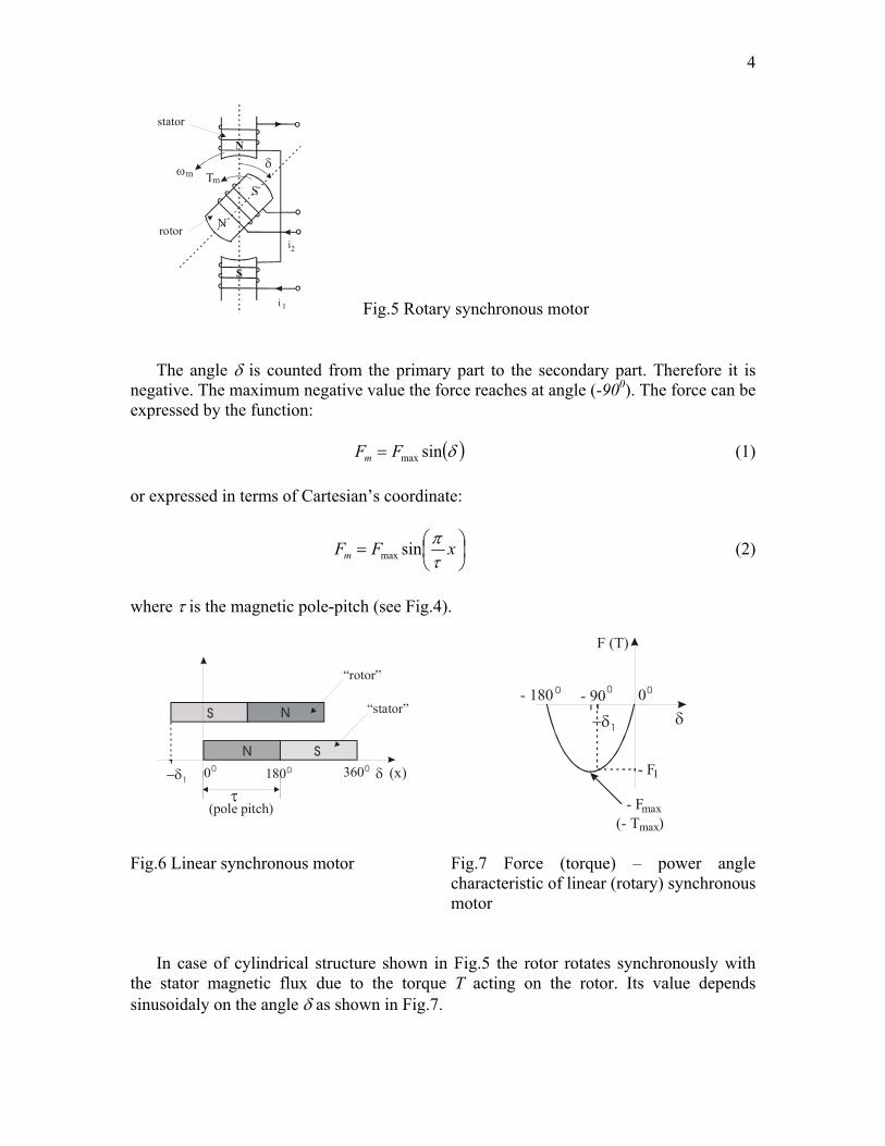
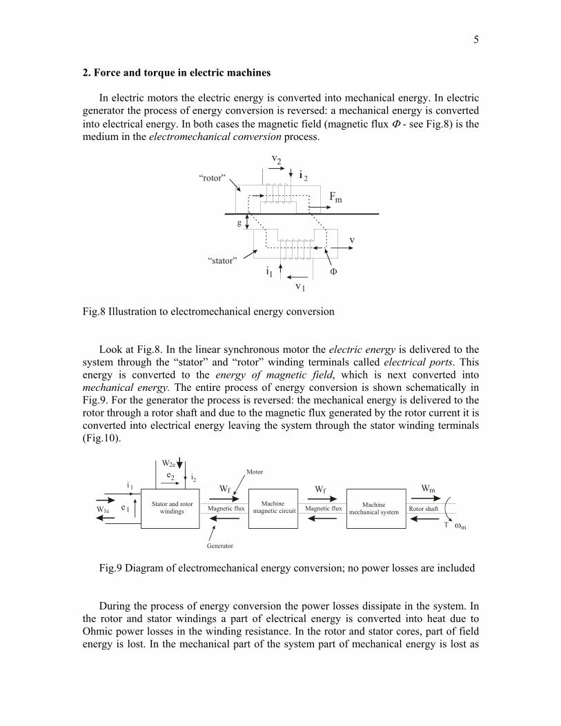
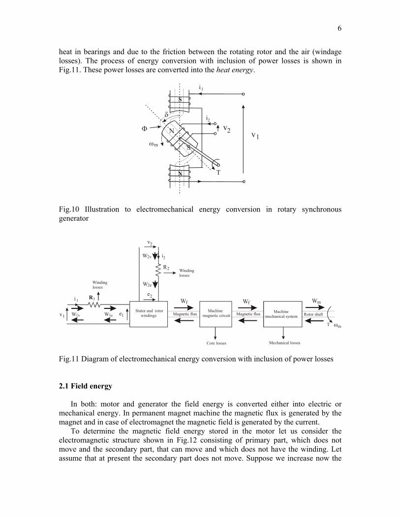
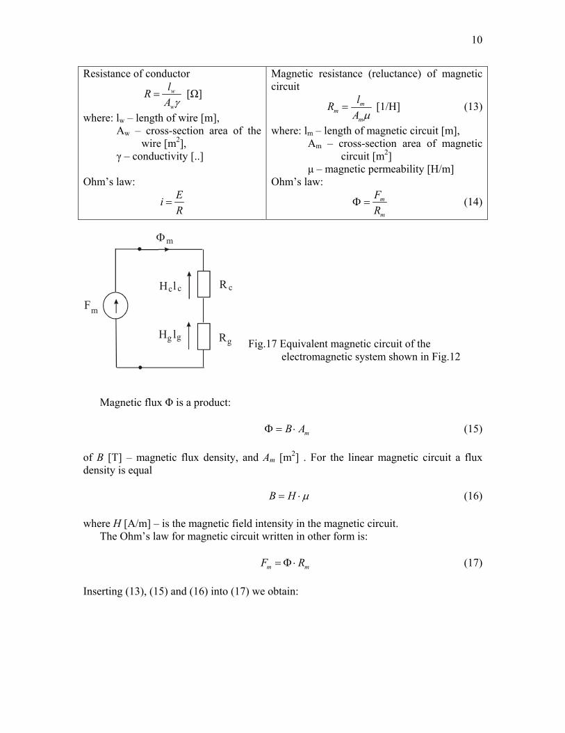
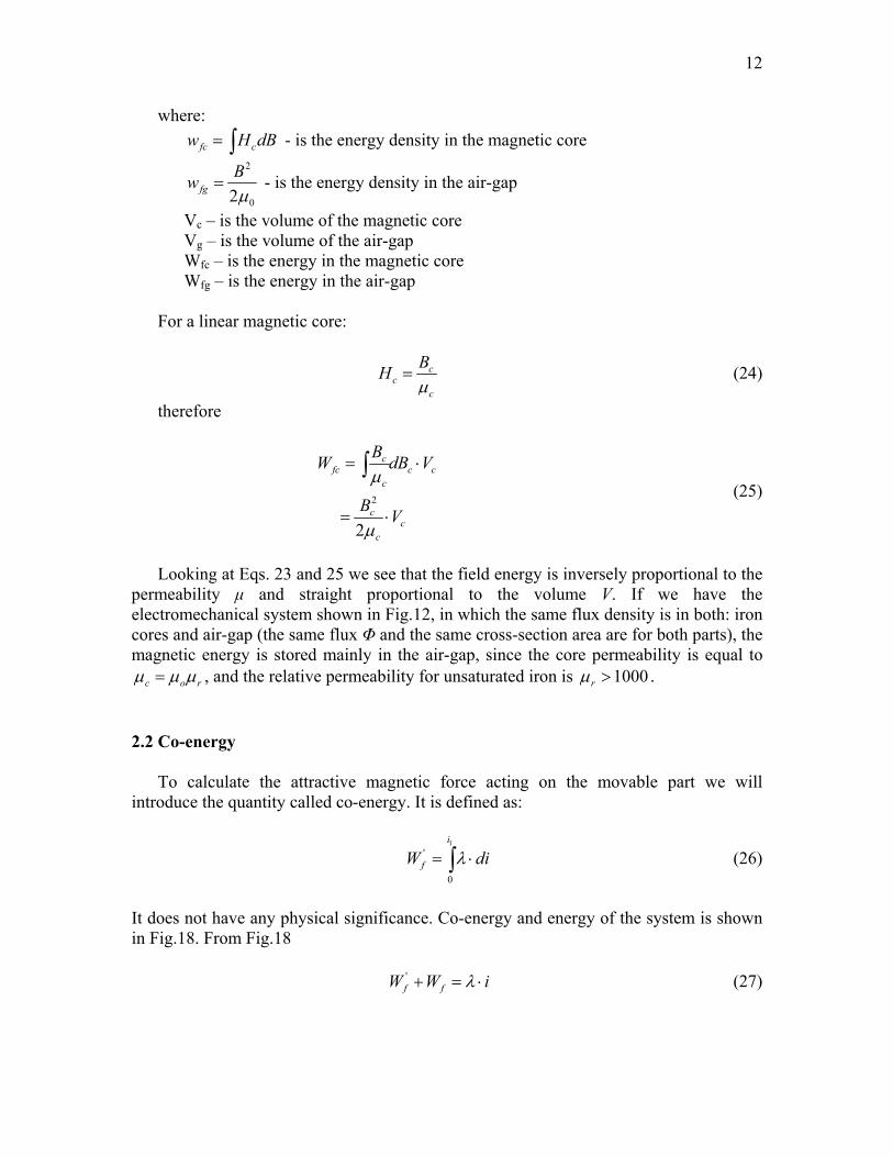
12
where
fc cw H dB= int - is the energy density in the magnetic core 2
02fgBwmicro
= - is the energy density in the air-gap
Vc ndash is the volume of the magnetic core Vg ndash is the volume of the air-gap Wfc ndash is the energy in the magnetic core Wfg ndash is the energy in the air-gap
For a linear magnetic core
cc
c
BHmicro
= (24)
therefore
2
2
cfc c c
c
cc
c
BW dB V
B V
micro
micro
= sdot
= sdot
int (25)
Looking at Eqs 23 and 25 we see that the field energy is inversely proportional to the
permeability micro and straight proportional to the volume V If we have the electromechanical system shown in Fig12 in which the same flux density is in both iron cores and air-gap (the same flux Φ and the same cross-section area are for both parts) the magnetic energy is stored mainly in the air-gap since the core permeability is equal to
c o rmicro micro micro= and the relative permeability for unsaturated iron is 1000rmicro gt
22 Co-energy
To calculate the attractive magnetic force acting on the movable part we will
introduce the quantity called co-energy It is defined as
1
0
i
fW diλ= sdotint (26)
It does not have any physical significance Co-energy and energy of the system is shown in Fig18 From Fig18
f fW W iλ+ = sdot (27)
13
If λ-i characteristic is nonlinear f fW Wgt (Fig19 ndash curve g1) but if λ-i characteristic
is linear (straight line g2) f fW W= If the air-gap increases from g1 to g2 and the current
remains unchanged the co-energy will decrease as shown in Fig19
i0
fW
fW lsquo
λ1
λ
i 1
λ
i
ggλ 1
21
0 i1
Wrsquof1
Wrsquof2
λ 2
Fig18 Field energy Wf and field co-energy Wfrsquo
Fig19 Field co-energy for two different values of air-gap in the system
23 Mechanical energy and forces Let us consider the system in Fig20 Let the secondary part moves from one position
(x = x1) to another position (x = x2) The λ-i characteristics of the system for these two positions are shown in Fig21 If the secondary part has moved slowly the current equal to i v R= remains the same at both positions in the steady state because the coil resistance does not change and the voltage is set to be constant
i R
v e
g
Fm
Secondarypart (movable)
Primarypart (stationary)
Φ
e
iR1 1
11 v
22
22
x1x2 0x Fig20 Electromechanical system with movable and stationary parts
14
λ
i
xx
b
ad
c
λ
λ1
2
1
2
0 i1
dWe
Fig21 Illustration to the magnetic force derivation The operation point has moved upward from point a rarr b During the motion
2
1
( )edW e i dt i d area abcdλ
λ
λ= sdot sdot = sdot =int int (28)
the increment of electric energy has been sent to the system The field energy has changed by the increment
(0 0 )fdW area bc ad= minus (29) The mechanical energy
( ) (0 ) (0 )(0 )
m e fdW dW dWarea abcd area ad area bcarea ab
= minus
= + minus=
(30)
is equal to the mechanical work done during the motion of the secondary part and it is represented by the shaded area in Fig21 This shaded area can be seen also as the increase in the co-energy
m fdW dW= (31) Since
m mdW f dx= (32)
the force fm that is causing differential displacement is
( ) fm
i const
W i xf
x=
part=
part (33)
15
231 Force in linear system Let us consider again the system shown in Fig20 The reluctance of the magnetic core path can be ignored due to the high value of microc (see Eq13) and the λ-i characteristic is assumed to be linear The coil inductance L1 depends on the reluctance of the magnetic circuit From Eqs3 and 14 we obtain
m
m
N FLR isdot
= (34)
From Eqs13 and 34 after transformation we obtain
2mN AL
gmicro
= (35)
That means that inductance L depends on length of the air-gap so it is the function of x co-ordinate (see Fig20) Thus for the idealized system
( )L x iλ = (36) where L(x) changes its value with the gap length Since the field co-energy is
0
i
fW diλ= sdotint (37)
after inserting Eq36 for λ we obtain
( )
( )
0
212
i
fW L x i di
L x i
= sdot
=
int (38)
The magnetic force acting on the secondary part we obtain from Eqs33 and 38
( )
( )
2
2
12
12
mi const
f L x ix
dL xi
dx
=
part = part
=
(39)
For a linear system the field energy is equal to the co-energy (Fig19 ndash line g2) thus
16
( ) 212f fW W L x i= = (40)
Force fm can be expressed also in terms of magnetic flux density in the air-gap Bg If we assume that Hc is negligible (due to high permeability microc of the core) then for mechanical system in Fig20 we obtain from Eq19
0
2 2gg
BNi H g g
micro= = (41)
and
0
2gBi g
Nmicro= (42)
From Eqs35 38 and 42 we obtain
2
0
22
gf g
BW A g
micro= sdot sdot (43)
The above expression can be obtained also from the field energy For the linear magnetic circuit
f fW W= therefore from Eq23 (for negligible magnetic energy stored in the core)
2
02
0
2
22
gf g
gg
BW V
BA g
micro
micro
= sdot
= sdot sdot
(44)
where Ag is the cross-section area of the air-gap
From Eqs33 and 43 the force acting on the secondary part is
2
0
2
0
22
22
gm g
gg
Bf A g
g
BA
micro
micro
part= sdot sdot part
= sdot
(45)
It means that the magnetic force is proportional to the magnetic flux density in square
The magnetic pressure Fm that is often used is calculated as the force per unit area of air-gap Thus from Eq45 we have (the cross-section area of the air-gap is 2Ag)
17
2
02g
m
BF
micro= (46)
The expression 45 can be used to calculate the force in all electromechanical devices where the magnetic flux density in the air-gap is known So it can also be applied to determine the driving force in all these primitive linear motors shown in Fgs1 - 4 Let us consider the reluctance linear ldquomotorrdquo shown in Fig22 The magnetic force acting on the ldquorotorrdquo (and the same force but in opposite direction acts on the ldquostatorrdquo) is expressed by Eq45 The driving force fx acting on the ldquorotorrdquo is the tangential (to x axis) component that can be determined from fm if we know the angle β or the mutual displacement ∆x between two motor parts
If we have the reluctance motor with the primary part as an electromagnet (Fig23) we can use formula 39 to determine the linear force fx acting on the secondary part The data that we have to know is the current i flowing in the ldquostatorrdquo winding and the inductance L(x) expressed as the function of x coordinate If the ldquorotorrdquo is infinitely long in x direction as in Fig24 then L = const with respect to x direction and according to Eq23 the force fx = 0 despite very strong attractive force fy acting on the ldquorotorrdquo
N SN
ldquorotorrdquo (Fe)
ldquostatorrdquo
B Sv
x
fmfm
fx
fyy
∆x
δ
Fig22 Force components in linear reluctance motor
i1
vN S
ldquostatorrdquo
ldquorotorrdquo fxx
y
Fig23 Force component Fx produced in the linear reluctance motor The Eqns39 and 45 for force was derived for the system with the coil wound on the primary part only We derive now the force equation for the linear system with the coil wound also on the secondary part (Fig20) as it is in synchronous linear motors shown in Fig8 To do this let us assume again that the secondary part does not move and the field energy is equal to the electric energy
18
1 1 2 2
1 1 2 2
f edW dW e i dt e i dti d i dλ λ
= = +
= + (47)
i1
vN S
ldquostatorrdquo
ldquorotorrdquo
fy
x
y
Fig24 No driving force in the motor with infinitely (very) long ldquorotorrdquo In the linear system (the λ-i characteristic is represented by the straight line see Fig13b) the flux linkages can be expressed in terms of inductances that are constant
1 11 11 12 2
2 21 1 22 2
L i L iL i L i
λλ
= += +
(48)
where L11 ndash is the self inductance of the excitation winding
L22 ndash is the self inductance of the moveable part winding L12 and L21 ndash are the mutual inductances between two windings
From Eqs33 and 34
( ) ( )( )
1 11 1 12 2 2 22 2 21 1
11 1 1 22 2 2 12 1 2
fdW i d L i L i i d L i L i
L i di L i di L d i i
= + + +
= + + (49)
The field energy is equal to the field co-energy for the linear systems Thus we have
( )1 2 1 2
11 1 1 22 2 2 12 1 2
0 0 0
2 211 1 22 2 12 1 2
1 12 2
i i i i
f fW W L i di L i di L d i i
L i L i L i i
= = + +
= + +
int int int (50)
In the system analyzed here the inductances depend on the value of an air-gap It
means that they are functions of position x of secondary part According to Eq33 the force developed by the linear system
19
( )
2 211 22 121 2 1 2
1 12 2
fm
i const
W i xf
x
dL dL dLi i i idx dx dx
=
part=
part
= + +
(51)
The first two terms are the two force components known as reluctance forces The third one is called an electromagnetic force This force exists even if self inductances do not depend on x co-ordinate it is if there are no two first components This type of situation exists in the system shown in Fig25 where either two or one of the part is infinitely (very) long When the secondary moves with respect to the primary self inductances of the coils remain unchanged and only the mutual magnetic coupling (mutual inductance) changes
i1
i2
Fig25 Coils in the infinitely long ldquostatorrdquo and ldquorotorrdquo cores
Equilibrium equations To analyze transients in the windings and dynamic behavior of the motors we have to
write equilibrium equations for electrical ports and mechanical port The equilibrium equations for electrical ports are terminal voltage equations for both primary and secondary windings written on the basis of the second (voltage) Kirhhoffrsquos law applied to equivalent circuit of both windings shown in Fig26 Equation for mechanical port is the equation of motion for mechanical system of the motor shown in Fig27 and written in accordance with the Newtonrsquos Law of Motion The equations written for the electromechanical system shown in Fig20 are as follows
- for electrical ports
11 1 1v R i
tλpart
= +part
(52)
22 2 2v R i
tλpart
= +part
(53)
- for mechanical port
20
2
2m Ld x dxf M D fdt dt
= + + (54)
where
M ndash is mass of the movable part D ndash friction coefficient of the movable secondary part fL ndash load force In the above voltage equations the terminal voltages are equal to the voltage drops
across the winding resistances and the voltages e1 and e2 (see Fig26) induced in the windings by the fluxes linked with them In the motion equation the electromagnetic force developed by the motor is equal to the inertia force friction force and load force
i R
v e e
iR1 1
11 v
22
2
Φ
2
M(x)
v Fig26 Equivalent circuit of the electromechanical system in Fig20
Fm
Secondarypart
D
v
Mmass F - inertiaMF - loadLF - frictionD
Fig27 Equivalent mechanical system of the electromechanical system in Fig20 The derivatives
( )( ) ( )( )
( ) ( ) ( ) ( )
11 1 12 211
11 121 211 1 12 2
L x i L x ie
t t tdL x dL xdi didx dxL x i L x i
dt dx dt dt dx dt
λ part partpart= = +
part part part
= + + +
(55)
21
( )( ) ( )( )
( ) ( ) ( ) ( )
22 2 21 122
22 212 122 2 21 1
L x i L x ie
t t tdL x dL xdi didx dxL x i L x i
dt dx dt dt dx dt
λ part partpart= = +
part part part
= + + +
(56)
Examples of electromechanical devices with a linear (oscillating) motion - transformer with moving coil (for secondary voltage variation) (Fig28)
R1
v1 L11
x
R 1i
2iR2R
L22
M(x)
v2
e 1
e 2
Voltage equations
tiRv
partpart
+= 1111
λ
tiRv
partpart
+= 2222
λ
since 1 11 11 12 2 2 21 1 22 2L i L i and L i L iλ λ= + = + and 11 22 12 21 ( )L L and L L M x= = are constant in
time
( )1 21 1 1 11
di div R i L M xdt dt
= + + or 1 1 1 1v R i e= +
( )2 12 2 2 22
di div R i L M xdt dt
= + + or 2 2 2 2v R i e= +
Fig28 Equivalent circuit of transformer
Changing the distance between the coils we influence M(x) and we change the
voltage e2 and v2 - jumping ring (Fig29)
v
C
Φ
ΦX
X
i1
i2
i1
Fig29 Jumping ring
22
Idea of operation Magnetic flux of the coil Φcoil induces the voltage E2 (and the current i2) in the ring The current i2 in the ring contributes to the flux Φring This flux opposes the flux Φcoil according to phasor diagram in Fig30b (the inductances L11 and E22 are assumed to be much greater than the resistances R1 and R2) As the result the ring is repelled out of the coil
(a) (b)
R1
v1 L1
f em
fg
x
R 1i
2iR2R
L2
M(x)
Aluminum ring
v = 02
C
E1
E2
Φ
V = E
I
E
ΦI
1 1
1
1
2
2
2R2ltlt L2
R1ltlt L1
Fig30 Equivalent circuit of the jumping ring (a) and its phasor diagram (b) When the distance between the coil and ring changes then the resultant inductance of
the coil is changing too If the capacitor C has the value that brings the coil circuit into resonance when the ring is at lowest position then the heavy coil current contributes to the strong force that repels the ring upwards When the ring is far from the coil the resonance disappears consequently the lifting force goes to zero and the ring falls down There the resonance occurs again and the ring is repelled again The resultant effect is the jumping ring The equivalent circuit of the device with jumping ring is shown in Fig30a
- induction linear oscillator (Fig31) The phenomenon described above is applied in induction oscillation motor shown
schematically in Fig31 Two coils are placed at the ends of the ferromagnetic bar Both
vC C
Fig31 Scheme of induction linear oscillator
23
are connected in parallel to the AC source via capacitors If the ring placed between them is close to one of the coil then the resonance occur in the coil and strong repulsion produced force throws the ring to the other coil When the ring appears close to this coil the resonance of this coil will contributes to the repulsion of the ring to the opposite coil Consequently the ring oscillates between the coils
- Reluctance linear oscillator (Fig32)
The ferromagnetic bar loosely placed in the coil is suspended by the attractive
magnetic force produced by the coil magnetic flux (Fig32a) When the bar moves in the coil the coil inductance changes its value If the capacitor connected in series to the coil is chosen to put the circuit into resonance when the bar is at lower position (see Fig32b) then due to the heavy resonance current a strong magnetic force pulls the bar upwards into the coil There the circuit is out of resonance and due to the small current (and no magnetic force at the center of the coil) the bar falls down When it comes at the end of the coil the resonance appears again pulling the bar upwards In consequence the bar will oscillate in vertical position
If the coil is placed in horizontal position as in Fig33 then the resonance current appear at both ends The bar will oscillate in horizontal position To increase the efficiency of the oscillator end-rings are placed at both ends (see Fig34) At the end of the bar track the kinetic energy of the moving bar is not lost but converted into the potential energy of the spring and next returned to the bar This reluctance oscillator is more efficient than the induction oscillator because there are no current losses in the moving part
(a) (b)
R1
v1 L1
f m
f g
xR 1i
D
R1
v1 L1
f m
f g
xR 1i
D
C
x2
1 0
Fig32 Circuit diagrams (a) ferromagnetic bar suspended by the magnetic field (b) electromagnetic device with jumping ferromagnetic bar
24
v
Ci
L(x)i(x)
0
x
x
0xr
Fig33 Scheme of the reluctance linear oscillator with the current and coil inductance characteristics
v
Ci
Fig34 Reluctance linear oscillator with end springs 232 Torque in rotating machines
Let us consider the rotating electromagnetic system shown in Fig35 in which the stator possesses winding 1 and the rotor ndash winding 2 The field co-energy is expressed by Eqn50 The torque developed by the motor is
25
( ) f
i const
W iT
θθ
=
part=
part (57)
From Eqs50 and 57
2 211 22 121 2 1 2
1 12 2
dL dL dLT i i i id d dθ θ θ
= + + (58)
i R
v
iR1 1
1v
22
2em
Rotor
Stator
θ
ω1
e2
Fig35 Rotary motor with salient pole stator and rotor The first two terms are reluctance torques and the third one is an electromagnetic torque For the motor with the round rotor (Fig36) there is no torque represented by the first term since the self inductance of the stator L11 does not depend on the position of the torque (the magnetic flux generated by the first winding does not change as the rotor rotates) Therefore the torque of this motor is described by the following equation
2 22 122 1 2
12
dL dLT i i id dθ θ
= + (59)
i
em
θ
ω
i1
1
2
e2
Fig36 Motor with the salient pole stator and round rotor
Suppose the stator has cylindrical structure and the rotor has salient magnetic poles as shown in Fig37 In such a motor known as synchronous motor with salient poles the
26
self inductance of the rotor winding L22 does not change as the rotor rotates Therefore the torque equation takes the form
2 11 121 1 2
12
dL dLT i i id dθ θ
= + (60)
The first term is the reluctance torque and the second one is known as a synchronous torque
i
m
Rotor
θ
ω
2
i1
Stator
Fig37 Motor with round stator and salient pole rotor Machines with cylindrical stator and rotor A scheme of cylindrical machine is shown in Fig38 The self inductances are constant and therefore no reluctance torque is produced The torque developed by the motor is
121 2
dLT i idθ
= (61)
i
m
θ
ω
2
i1
Fig38 Motor with cylindrical stator and rotor Let the mutual inductance changes sinusoidally
27
12 cosL M θ= (62) where M ndash is the peak value of mutual inductance
θ ndash is the angle between the magnetic axis of the stator and rotor windings
Let the currents in the two windings be
1 1 1cosmi I tω= (63)
( )2 2 2cosmi I tω α= + (64) The position of the rotor with respect to the stator depends on rotor speed and is
mtθ ω δ= + (65) where ωm ndash is the angular velocity of the rotor
δ ndash is the rotor position at t = 0 From Eqns61 62 63 64 and 56 we have
( ) ( )
( )( )( )( )( )( )( )( )
1 2 1 2
1 21 2
1 2
1 2
1 2
cos cos sin
sin4
sin
sin
sin
m m m
m mm
m
m
m
T I I M t t tI I M t
t
t
t
ω ω α ω δ
ω ω ω α δ
ω ω ω α δ
ω ω ω α δ
ω ω ω α δ
= minus + +
= minus + + + +
+ minus + minus + + + minus minus + + minus minus + +
(66)
The torque is the sum of four components which vary sinusoidally with time Therefore the average value of each component is zero unless the coefficients of t are zero Thus the average torque will be nonzero if
( )1 2mω ω ω= plusmn plusmn (67) The machine will develop average torque if it rotates in either direction at a speed that is equal to the sum or difference of the angular frequencies 2 fω π= of the stator and the rotor currents
1 2mω ω ω= plusmn (68) There are two practical cases
1) ω2 = 0 α = 0 ωm = ω1 (single-phase synchronous machine) Rotor carries dc current stator ac current
28
For these conditions from Eqn66
( ) 1 21sin 2 sin
2m mI I MT tω δ δ= minus + + (69)
The instantaneous torque is pulsating It will be constant for poly-phase machine
To find the average torque from Eqn69 we see that average of ( )1sin 2 tω δ+ is zero It means the average torque is
1 2 sin
2avI I MT δ= minus (70)
If ωm = 0 (at starting) the (single-phase) machine does not develop the average
torque
2) ωm = ω1 - ω2 (asynchronous single-phase motor) Both stator and the rotor carry ac currents at different frequencies and rotor speed ωm ne ω1 and ωm ne ω2 From Eq66
( ) ( )( ) ( )
1 21 2
1 2
sin 2 sin 22
sin 2 2 sin
m mI I MT t t
t t
ω α δ ω α δ
ω ω α δ α δ
= minus + + + minus minus +
+ minus minus + + + (71)
The instantaneous torque is pulsating (it is constant in poly-phase motor) The
average value of the torque is
( )1 2 sin4
m mav
I I MT α δ= minus + (72)
At ωm = 0 the average torque is zero A single-phase machine should be brought
to the speed different than 0 so it can produce an average torque This is the principle of operation of induction motor
Equilibrium equations Similar as for linear motor the equilibrium equations for rotating machine are as
follows - for electrical ports voltage equations (the same as Eqns52 and 53)
1
1 1 1v R itλpart
= +part
(73)
29
22 2 2v R i
tλpart
= +part
(74)
The derivatives
( )( ) ( )( )
( ) ( ) ( ) ( )
11 1 12 21
11 121 211 1 12 2
L i L it t t
dL dLdi d di dL i L idt d dt dt d dt
θ θλ
θ θθ θθ θθ θ
part partpart= +
part part part
= + + +
(75)
( )( ) ( )( )
( ) ( ) ( ) ( )
22 2 21 12
22 212 122 2 21 1
L i L it t t
dL dLdi d di dL i L idt d dt dt d dt
θ θλ
θ θθ θθ θθ θ
part partpart= +
part part part
= + + +
(76)
The term mtθ ωpart
=part
is the angular speed of the rotor For the motor considered the
mutual inductances L12 = L21 = M thus
( ) ( ) ( ) ( )111 1 21 11 1 2m m
dL dMdi die L i M it dt d dt d
θ θλ θ ω θ ωθ θ
part= = + + +
part (77)
( ) ( ) ( ) ( )222 2 12 22 2 1m m
dL dMdi die L i M it dt d dt d
θ θλ θ ω θ ωθ θ
part= = + + +
part (78)
The voltages induced in the windings (see Fig36) form two groups The first one
contains the voltages
( ) ( )1 21 11t
di die L Mdt dt
θ θ= + (79)
( ) ( )2 12 22t
di die L Mdt dt
θ θ= + (80)
induced due to the variation in time of the magnetic fluxes represented by the currents that generate them These types of voltages are induced in transformers (index t) The second group
( ) ( )11
1 1 2r m m
dL dMe i i
d dθ θ
ω ωθ θ
= + (81)
( ) ( )22
2 2 1r m m
dL dMe i i
d dθ θ
ω ωθ θ
= + (82)
30
are the voltages induced by the rotation of the rotor In that number the first terms are the voltages induced by the saliency of the rotor and do not exist in the motor with cylindrical stator and the rotor (see Fig38) The second terms are the voltages induced by the mutual rotation of the two windings
- for mechanical port motion equation (Fig39)
2
2 s ld dT J D T Tdt dt
θ θ= + + + (83)
where J ndash moment of inertia of the rotor D ndash friction coefficient of the rotor Tl ndash load torque Ts ndash torsional torque (see Fig40 ndash two torques act in opposite directions and they
twist the shafts by angle ∆θ) which is due to the rotor shaft elasticity and is given by
( )s sT K θ= ∆ (84)
where Ks is the torsional coefficient
Tm
TL
Motor Load
TDTJ
mω
Fig39 Equivalent diagram for mechanical system of the rotary motor Tm ndash
electromagnetic torque TJ ndash inertia torque TD ndash friction torque TL ndash load torque
∆θ
Tm
TL
Motor Load
Fig40 Twist (by the angle ∆θ) of the elastic shaft caused by electromagnetic torque of
the motor Tm and load torque TL acting in oposite direction
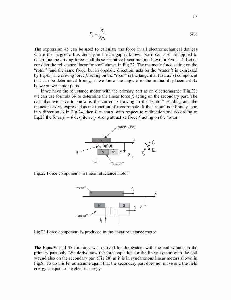
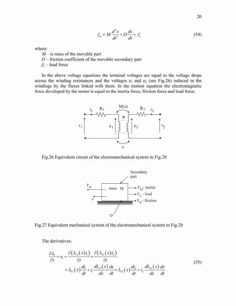

22
Idea of operation Magnetic flux of the coil Φcoil induces the voltage E2 (and the current i2) in the ring The current i2 in the ring contributes to the flux Φring This flux opposes the flux Φcoil according to phasor diagram in Fig30b (the inductances L11 and E22 are assumed to be much greater than the resistances R1 and R2) As the result the ring is repelled out of the coil
(a) (b)
R1
v1 L1
f em
fg
x
R 1i
2iR2R
L2
M(x)
Aluminum ring
v = 02
C
E1
E2
Φ
V = E
I
E
ΦI
1 1
1
1
2
2
2R2ltlt L2
R1ltlt L1
Fig30 Equivalent circuit of the jumping ring (a) and its phasor diagram (b) When the distance between the coil and ring changes then the resultant inductance of
the coil is changing too If the capacitor C has the value that brings the coil circuit into resonance when the ring is at lowest position then the heavy coil current contributes to the strong force that repels the ring upwards When the ring is far from the coil the resonance disappears consequently the lifting force goes to zero and the ring falls down There the resonance occurs again and the ring is repelled again The resultant effect is the jumping ring The equivalent circuit of the device with jumping ring is shown in Fig30a
- induction linear oscillator (Fig31) The phenomenon described above is applied in induction oscillation motor shown
schematically in Fig31 Two coils are placed at the ends of the ferromagnetic bar Both
vC C
Fig31 Scheme of induction linear oscillator
23
are connected in parallel to the AC source via capacitors If the ring placed between them is close to one of the coil then the resonance occur in the coil and strong repulsion produced force throws the ring to the other coil When the ring appears close to this coil the resonance of this coil will contributes to the repulsion of the ring to the opposite coil Consequently the ring oscillates between the coils
- Reluctance linear oscillator (Fig32)
The ferromagnetic bar loosely placed in the coil is suspended by the attractive
magnetic force produced by the coil magnetic flux (Fig32a) When the bar moves in the coil the coil inductance changes its value If the capacitor connected in series to the coil is chosen to put the circuit into resonance when the bar is at lower position (see Fig32b) then due to the heavy resonance current a strong magnetic force pulls the bar upwards into the coil There the circuit is out of resonance and due to the small current (and no magnetic force at the center of the coil) the bar falls down When it comes at the end of the coil the resonance appears again pulling the bar upwards In consequence the bar will oscillate in vertical position
If the coil is placed in horizontal position as in Fig33 then the resonance current appear at both ends The bar will oscillate in horizontal position To increase the efficiency of the oscillator end-rings are placed at both ends (see Fig34) At the end of the bar track the kinetic energy of the moving bar is not lost but converted into the potential energy of the spring and next returned to the bar This reluctance oscillator is more efficient than the induction oscillator because there are no current losses in the moving part
(a) (b)
R1
v1 L1
f m
f g
xR 1i
D
R1
v1 L1
f m
f g
xR 1i
D
C
x2
1 0
Fig32 Circuit diagrams (a) ferromagnetic bar suspended by the magnetic field (b) electromagnetic device with jumping ferromagnetic bar
24
v
Ci
L(x)i(x)
0
x
x
0xr
Fig33 Scheme of the reluctance linear oscillator with the current and coil inductance characteristics
v
Ci
Fig34 Reluctance linear oscillator with end springs 232 Torque in rotating machines
Let us consider the rotating electromagnetic system shown in Fig35 in which the stator possesses winding 1 and the rotor ndash winding 2 The field co-energy is expressed by Eqn50 The torque developed by the motor is
25
( ) f
i const
W iT
θθ
=
part=
part (57)
From Eqs50 and 57
2 211 22 121 2 1 2
1 12 2
dL dL dLT i i i id d dθ θ θ
= + + (58)
i R
v
iR1 1
1v
22
2em
Rotor
Stator
θ
ω1
e2
Fig35 Rotary motor with salient pole stator and rotor The first two terms are reluctance torques and the third one is an electromagnetic torque For the motor with the round rotor (Fig36) there is no torque represented by the first term since the self inductance of the stator L11 does not depend on the position of the torque (the magnetic flux generated by the first winding does not change as the rotor rotates) Therefore the torque of this motor is described by the following equation
2 22 122 1 2
12
dL dLT i i id dθ θ
= + (59)
i
em
θ
ω
i1
1
2
e2
Fig36 Motor with the salient pole stator and round rotor
Suppose the stator has cylindrical structure and the rotor has salient magnetic poles as shown in Fig37 In such a motor known as synchronous motor with salient poles the
26
self inductance of the rotor winding L22 does not change as the rotor rotates Therefore the torque equation takes the form
2 11 121 1 2
12
dL dLT i i id dθ θ
= + (60)
The first term is the reluctance torque and the second one is known as a synchronous torque
i
m
Rotor
θ
ω
2
i1
Stator
Fig37 Motor with round stator and salient pole rotor Machines with cylindrical stator and rotor A scheme of cylindrical machine is shown in Fig38 The self inductances are constant and therefore no reluctance torque is produced The torque developed by the motor is
121 2
dLT i idθ
= (61)
i
m
θ
ω
2
i1
Fig38 Motor with cylindrical stator and rotor Let the mutual inductance changes sinusoidally
27
12 cosL M θ= (62) where M ndash is the peak value of mutual inductance
θ ndash is the angle between the magnetic axis of the stator and rotor windings
Let the currents in the two windings be
1 1 1cosmi I tω= (63)
( )2 2 2cosmi I tω α= + (64) The position of the rotor with respect to the stator depends on rotor speed and is
mtθ ω δ= + (65) where ωm ndash is the angular velocity of the rotor
δ ndash is the rotor position at t = 0 From Eqns61 62 63 64 and 56 we have
( ) ( )
( )( )( )( )( )( )( )( )
1 2 1 2
1 21 2
1 2
1 2
1 2
cos cos sin
sin4
sin
sin
sin
m m m
m mm
m
m
m
T I I M t t tI I M t
t
t
t
ω ω α ω δ
ω ω ω α δ
ω ω ω α δ
ω ω ω α δ
ω ω ω α δ
= minus + +
= minus + + + +
+ minus + minus + + + minus minus + + minus minus + +
(66)
The torque is the sum of four components which vary sinusoidally with time Therefore the average value of each component is zero unless the coefficients of t are zero Thus the average torque will be nonzero if
( )1 2mω ω ω= plusmn plusmn (67) The machine will develop average torque if it rotates in either direction at a speed that is equal to the sum or difference of the angular frequencies 2 fω π= of the stator and the rotor currents
1 2mω ω ω= plusmn (68) There are two practical cases
1) ω2 = 0 α = 0 ωm = ω1 (single-phase synchronous machine) Rotor carries dc current stator ac current
28
For these conditions from Eqn66
( ) 1 21sin 2 sin
2m mI I MT tω δ δ= minus + + (69)
The instantaneous torque is pulsating It will be constant for poly-phase machine
To find the average torque from Eqn69 we see that average of ( )1sin 2 tω δ+ is zero It means the average torque is
1 2 sin
2avI I MT δ= minus (70)
If ωm = 0 (at starting) the (single-phase) machine does not develop the average
torque
2) ωm = ω1 - ω2 (asynchronous single-phase motor) Both stator and the rotor carry ac currents at different frequencies and rotor speed ωm ne ω1 and ωm ne ω2 From Eq66
( ) ( )( ) ( )
1 21 2
1 2
sin 2 sin 22
sin 2 2 sin
m mI I MT t t
t t
ω α δ ω α δ
ω ω α δ α δ
= minus + + + minus minus +
+ minus minus + + + (71)
The instantaneous torque is pulsating (it is constant in poly-phase motor) The
average value of the torque is
( )1 2 sin4
m mav
I I MT α δ= minus + (72)
At ωm = 0 the average torque is zero A single-phase machine should be brought
to the speed different than 0 so it can produce an average torque This is the principle of operation of induction motor
Equilibrium equations Similar as for linear motor the equilibrium equations for rotating machine are as
follows - for electrical ports voltage equations (the same as Eqns52 and 53)
1
1 1 1v R itλpart
= +part
(73)
29
22 2 2v R i
tλpart
= +part
(74)
The derivatives
( )( ) ( )( )
( ) ( ) ( ) ( )
11 1 12 21
11 121 211 1 12 2
L i L it t t
dL dLdi d di dL i L idt d dt dt d dt
θ θλ
θ θθ θθ θθ θ
part partpart= +
part part part
= + + +
(75)
( )( ) ( )( )
( ) ( ) ( ) ( )
22 2 21 12
22 212 122 2 21 1
L i L it t t
dL dLdi d di dL i L idt d dt dt d dt
θ θλ
θ θθ θθ θθ θ
part partpart= +
part part part
= + + +
(76)
The term mtθ ωpart
=part
is the angular speed of the rotor For the motor considered the
mutual inductances L12 = L21 = M thus
( ) ( ) ( ) ( )111 1 21 11 1 2m m
dL dMdi die L i M it dt d dt d
θ θλ θ ω θ ωθ θ
part= = + + +
part (77)
( ) ( ) ( ) ( )222 2 12 22 2 1m m
dL dMdi die L i M it dt d dt d
θ θλ θ ω θ ωθ θ
part= = + + +
part (78)
The voltages induced in the windings (see Fig36) form two groups The first one
contains the voltages
( ) ( )1 21 11t
di die L Mdt dt
θ θ= + (79)
( ) ( )2 12 22t
di die L Mdt dt
θ θ= + (80)
induced due to the variation in time of the magnetic fluxes represented by the currents that generate them These types of voltages are induced in transformers (index t) The second group
( ) ( )11
1 1 2r m m
dL dMe i i
d dθ θ
ω ωθ θ
= + (81)
( ) ( )22
2 2 1r m m
dL dMe i i
d dθ θ
ω ωθ θ
= + (82)
30
are the voltages induced by the rotation of the rotor In that number the first terms are the voltages induced by the saliency of the rotor and do not exist in the motor with cylindrical stator and the rotor (see Fig38) The second terms are the voltages induced by the mutual rotation of the two windings
- for mechanical port motion equation (Fig39)
2
2 s ld dT J D T Tdt dt
θ θ= + + + (83)
where J ndash moment of inertia of the rotor D ndash friction coefficient of the rotor Tl ndash load torque Ts ndash torsional torque (see Fig40 ndash two torques act in opposite directions and they
twist the shafts by angle ∆θ) which is due to the rotor shaft elasticity and is given by
( )s sT K θ= ∆ (84)
where Ks is the torsional coefficient
Tm
TL
Motor Load
TDTJ
mω
Fig39 Equivalent diagram for mechanical system of the rotary motor Tm ndash
electromagnetic torque TJ ndash inertia torque TD ndash friction torque TL ndash load torque
∆θ
Tm
TL
Motor Load
Fig40 Twist (by the angle ∆θ) of the elastic shaft caused by electromagnetic torque of
the motor Tm and load torque TL acting in oposite direction
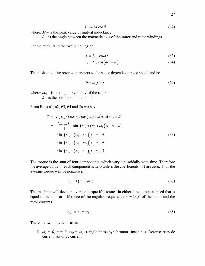