30 BOOTSTRAPPING DENSITY-WEIGHTED AVERAGE DERIVATIVES€¦ · BOOTSTRAPPING DENSITY-WEIGHTED...

Econometric Theory, 30, 2014, 1135–1164.doi:10.1017/S0266466614000127

BOOTSTRAPPINGDENSITY-WEIGHTED AVERAGE

DERIVATIVES

MATIAS D. CATTANEODepartment of Economics, University of Michigan

RICHARD K. CRUMPCapital Markets Function, Federal Reserve Bank of New York

MICHAEL JANSSONDepartment of Economics, UC Berkeley and CREATES

We investigate the properties of several bootstrap-based inference proceduresfor semiparametric density-weighted average derivatives. The key innovation inthis paper is to employ an alternative asymptotic framework to assess the prop-erties of these inference procedures. This theoretical approach is conceptuallydistinct from the traditional approach (based on asymptotic linearity of the esti-mator and Edgeworth expansions), and leads to different theoretical prescriptionsfor bootstrap-based semiparametric inference. First, we show that the conventionalbootstrap-based approximations to the distribution of the estimator and its classicalstudentized version are both invalid in general. This result shows a fundamental lackof “robustness” of the associated, classical bootstrap-based inference procedureswith respect to the bandwidth choice. Second, we present a new bootstrap-basedinference procedure for density-weighted average derivatives that is more “robust”to perturbations of the bandwidth choice, and hence exhibits demonstrable supe-rior theoretical statistical properties over the traditional bootstrap-based inferenceprocedures. Finally, we also examine the validity and invalidity of related bootstrap-based inference procedures and discuss additional results that may be of independentinterest. Some simulation evidence is also presented.

1. INTRODUCTION

The bootstrap has gained great popularity in modern econometrics and statistics.1

In semiparametric problems, where estimators of a finite-dimensional parame-ter of interest involve a nonparametric estimator of an unknown function, the

The authors thank Joel Horowitz, Guido Imbens, Lutz Kilian, Demian Pouzo, Rocio Titiunik, seminar participantsat Columbia/NYU, Duke, Harvard, LSE, Michigan, Northwestern, Rochester, and USC, and conference participantsat the 2010 Econometric Society World Congress for comments. We also thank the co-editor, Yoon-Jae Whang, andtwo anonymous referees for their suggestions. The first author gratefully acknowledges financial support from theNational Science Foundation (SES 0921505 and SES 1122994). The third author gratefully acknowledges finan-cial support from the National Science Foundation (SES 0920953 and SES 1124174) and the research support ofCREATES (funded by the Danish National Research Foundation).

c© Cambridge University Press 2014 1135

1136 MATIAS D. CATTANEO ET AL.

bootstrap is attractive, because of its ability to approximate the distribution ofthe semiparametric estimator in cases where variance estimation is difficult (e.g.,Chen, Linton, and van Keilegom, 2003; Cheng and Huang, 2010). Even whenvariance estimation is relatively straightforward, the bootstrap is potentially usefulin semiparametrics, because it may provide more accurate approximations to thedistributions of (asymptotically) pivotal quantities such as studentized estimators,whenever it achieves asymptotic refinements similar to those well-established inparametric problems (e.g., Hall, 1992).

The kernel-based density-weighted average derivative estimator of Powell,Stock, and Stoker (1989) is one of the few semiparametric estimators for whichthe bootstrap has been shown to offer asymptotic refinements. Nishiyama andRobinson (2005) recently showed that a suitably implemented version of the non-parametric bootstrap provides a distributional approximation for the classical stu-dentized test statistic that is superior to the standard Gaussian approximation. Inthis paper we revisit this problem and obtain new results that can be viewed as acautionary tale regarding “the potential for bootstrap-based inference to (. . . ) pro-vide improvements in moderate-sized samples” (Nishiyama and Robinson, 2005,p. 927). We present simulation evidence that appears hard to reconcile with thetheoretical results establishing asymptotic refinements of the bootstrap in thissemiparametric context and develop an alternative theory-based explanation ofthis evidence. In addition, we use our theoretical framework to derive results foralternative bootstrap-based inference procedures and to show, among other things,that there exists a valid bootstrap-based inference procedure that dominates theone proposed by Nishiyama and Robinson (2005), a theory-based prediction alsoborne out in our simulations.

The traditional approach to evaluating the accuracy of bootstrap-based infer-ence procedures (in parametric and semiparametric problems) relies on asymp-totic linearity of estimators and employs Edgeworth expansions to elucidate therole of “higher-order” terms in the distributional approximation of the associatedtest statistics. For the density-weighted average derivative estimator, Nishiyamaand Robinson (2005) used this traditional approach to demonstrate the abilityof a bootstrap-based inference procedure to deliver asymptotic refinements. Incontrast, we propose in this paper to employ an alternative (first-order) distri-butional approach to examine the properties of bootstrap-based inference pro-cedures, which retains some terms that are asymptotically negligible when theestimator is asymptotically linear but can be first-order otherwise. This alternativeapproach accommodates, but does not require, certain departures from asymptoticlinearity, namely those that occur when the bandwidth of the nonparametric esti-mator vanishes too rapidly for asymptotic linearity to hold. Thus, we refer to thisapproach as a “small bandwidth” approach (Cattaneo, Crump and Jansson 2010;2014).

Although similar in spirit to the Edgeworth expansion approach to im-prove asymptotic approximations, our small bandwidth approach is conceptu-ally distinct and leads to different theoretical prescriptions for bootstrap-based

BOOTSTRAPPING DENSITY-WEIGHTED AVERAGE DERIVATIVES 1137

semiparametric inference. In particular, Theorem 1 finds that the conventionalbootstrap-based approximations to the distribution of the kernel-based semipara-metric estimator and the associated studentized version of this estimator employ-ing the traditional (jackknife) variance estimator are both invalid in general. Onthe other hand, Theorem 2 establishes consistency of the bootstrap approxima-tion to the distribution of the semiparametric estimator when studentized by adifferent, bias-corrected variance estimator. This alternative variance estimator isone for which the resulting studentized statistic is asymptotically standard nor-mal even when asymptotic linearity fails. However, and perhaps surprisingly,Theorem 3 shows that pivotality of the studentized estimator is not sufficient forbootstrap validity: a variance estimator is exhibited which renders the associatedstudentized statistic asymptotically standard normal even when asymptotic lin-earity fails, but nonetheless the standard bootstrap provides a valid distributionalapproximation for this asymptotically pivotal statistic only when asymptoticlinearity holds.

These results have some interesting theoretical implications. First, our find-ings shed new light on the properties of the bootstrap and some of its variantsin the context of semiparametric inference, documenting and highlighting, in par-ticular, a fragility of traditional bootstrap-based distributional approximations forkernel-based semiparametric statistics with respect to perturbations of the band-width choice (see Section 4.4 for further discussion on this point). Second, ourresults also include a new bootstrap-based inference procedure for density-weighted average derivatives which is more “robust” to perturbations of the band-width choice, and hence exhibiting theoretically demonstrable superior statisticalproperties over the traditional bootstrap-based inference procedures.

The remainder of the paper is organized as follows. Section 2 introduces themodel, summarizes some theoretical results available in the literature, and pro-vides a motivation for our work using a small-scale simulation study. Section 3reviews our alternative approach based on the small bandwidth framework anddevelops the main theoretical tools needed to study the bootstrap. Section 4 in-cludes the main results of the paper, while Section 5 concludes and discussesother contexts where our results could be applied. The Appendix contains briefmathematical proofs, but the supplemental appendix includes a detailed develop-ment of our results.

2. SETUP AND MOTIVATION

We assume throughout that zi = (yi , x ′i )

′, i = 1, . . . ,n, is a random sample ofz = (y, x ′)′, where y ∈ R is a dependent variable and x ∈ Rd is a continuous ex-planatory variable with density f (·). The density-weighted average derivative ofthe regression function g(x) = E[y|x] is θ = E[ f (x)∂g(x)/∂x]; see, e.g., Stoker(1986). (Detailed regularity conditions are given in the following section, butomitted here to ease the discussion.) Models where this estimand is of inter-est include single-index limited dependent variable models, generalized partially


linear models, and other related semilinear single-index generalized additive andnonadditive models. For example, suppose g(·) is of the form g(x) = G

(x ′

1β, x2)

with G(·) unknown and x partitioned as x = (x ′

1, x ′2

)′. Then, partitioning θ con-

formably with x as θ = (θ ′

1,θ′2

)′, the index parameter β is proportional to θ1 withproportionality factor E

[f (x)G1(x ′

1β, x2)]

where G1(u, x2) = ∂G(u, x2)/∂u.Powell, Stock, and Stoker (1989, henceforth PSS) noted that θ =

−2E [y∂ f (x)/∂x], and hence proposed the kernel-based estimator

θn = −21

n

n∑i=1

yi∂

∂xfn,i (xi ), fn,i (x) = 1

n −1

n∑j=1, j �=i

1

hdn

K

(xj − x

hn

),

where K :Rd →R is a kernel function and hn is a vanishing (positive) bandwidthsequence. Having subsequently been studied by Hardle and Tsybakov (1993),Robinson (1995), Powell and Stoker (1996), Nishiyama and Robinson (2000,2001, 2005), and many others, this estimator is one of the most widely investi-gated estimators in the semiparametrics literature.

Under conditions similar to those discussed below, PSS showed that θn

is asymptotically linear with influence function L(z) = 2(∂[ f (x)g(x)]/∂x −y∂ f (x)/∂x − θ); that is,

√n(θn − θ) = 1√

n

n∑i=1

L(zi )+op(1)�N (0,�), � = E[L(z)L(z)′]

, (1)

where � denotes weak convergence. (Throughout the paper limits are taken asn → ∞ unless otherwise noted.) PSS also exhibited a consistent estimator �n

of �. Defining V0,n = n−1�n , these results imply, in particular, that V−1/2

0,n (θn −θ)� N (0, Id), a result that can be used to construct asymptotically valid andeasily implemented confidence intervals for θ .

Although asymptotically valid, the distributional approximation

V−1/2

0,n

(θn − θ

) a∼ N (0, Id) might be suspected to be somewhat inaccuratein samples of moderate size due to the presence of the nonparametric es-timator of (the derivative of) the density f (·). In particular, folklore andsimulation evidence suggests that the distributional properties of kernel-basedestimators such as θn , and studentized versions thereof, can be rather sen-sitive to the choice of bandwidth hn . Motivated by concerns of this nature,Nishiyama and Robinson (2000, 2001) developed valid Edgeworth expan-

sions for statistics of the form λ′(θn − θ)/

√λ′V0,nλ with λ ∈ Rd and found

that in general the magnitude of the error in the distributional approximation

V−1/2

0,n (θn − θ)a∼ N (0, Id) depends on both the sample size and the band-

width, this error vanishing at a conventional parametric rate n−1/2 only inexceptional circumstances. Subsequently, Nishiyama and Robinson (2005,henceforth NR) developed more detailed expansions and showed that thenonparametric bootstrap provides approximations to the sampling distribution of


(a possibly bias-corrected version of) λ′(θn − θ)/

√λ′V0,nλ that are not merely

asymptotically valid, but actually capable of achieving asymptotic refinements.It is tempting to interpret the latter result as evidence that even in samples of

moderate size, highly accurate confidence intervals for θ can be constructed usingthe bootstrap. To investigate the extent to which this interpretation is warranted,we conducted a Monte Carlo experiment to evaluate the performance of the stan-dard normal and bootstrap approximations to the distribution of V

−1/2

0,n (θn − θ).Following NR, the simulation study uses a Tobit model yi = yi 1(yi > 0) withyi = x ′

iβ + εi , εi ∼N (0,1) independent of the bivariate vector xi , and 1(·) rep-resenting the indicator function. We set β = (1,1)′ and consider two models:Model 1, also used by NR, employs (x1i , x2i )

′∼N (0, I2) , while Model 2 intro-

duces asymmetry in the regressor distribution by employing x1i ∼ (χ4 − 4)/√

8,x2i ∼ N (0,1), and x1i ⊥⊥ x2i , where χ4 denotes a chi-squared random variablewith 4 degrees of freedom. The estimator θn is implemented using a fourth-orderGaussian product kernel (i.e., P = 4 in Assumption K below). We set λ = (1,0)′and consider three 95% confidence intervals:

CI0 =[

λ′θn −1.96√

λ′V0,nλ, λ′θn +1.96√

λ′V0,nλ

],

CI∗0 =[

λ′θn − c∗0,97.5

√λ′V0,nλ, λ′θn − c∗

0,2.5

√λ′V0,nλ

],

CI∗0,BC =[

λ′(θn − Bn)− c∗0,97.5

√λ′V0,nλ, λ′(θn − Bn)− c∗

0,2.5

√λ′V0,nλ

],

where c∗0,α denotes the αth percentile of the bootstrap approximation and Bn de-

notes a bias-correction estimate, both implemented as in NR. We conducted 3,000simulations, each with a sample size n = 1,000 and 2,000 bootstrap replications.

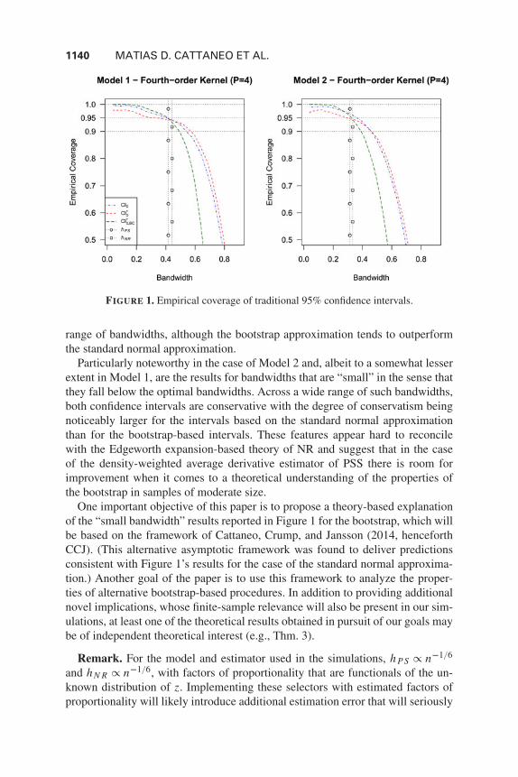
Figure 1 presents a summary of the Monte Carlo results. To investigate the sen-sitivity of the empirical coverage probabilities with respect to the bandwidth, theseresults are presented for a grid of possible bandwidth choices. This figure includestwo horizontal lines at 0.90 and at the nominal coverage rate 0.95 for reference,and also plots as vertical lines two (infeasible) bandwidth choices available in theliterature proposed by Powell and Stoker (1996) and NR, respectively, denotedh P S and hN R .

In perfect agreement with the theoretical findings of NR, the results for Model 1indicate that the bootstrap-based confidence intervals without bias-correction(CI∗0) are more accurate than those based on a standard normal approximation(CI0) and, in particular, that these bootstrap-based confidence intervals are highlyaccurate across a nontrivial range of bandwidths. (CI∗0,BC do not perform wellwhen the bias-correction is estimated.) On the other hand, the results for Model 2are much less encouraging, indicating, in particular, that the impressive findingsabout the bootstrap in Model 1 are to some extent an artifact of the particular dis-tributional assumption made on the part of the regressors in that model. Specifi-cally, in the case of Model 2 both approximations are inaccurate outside a narrow


FIGURE 1. Empirical coverage of traditional 95% confidence intervals.

range of bandwidths, although the bootstrap approximation tends to outperformthe standard normal approximation.

Particularly noteworthy in the case of Model 2 and, albeit to a somewhat lesserextent in Model 1, are the results for bandwidths that are “small” in the sense thatthey fall below the optimal bandwidths. Across a wide range of such bandwidths,both confidence intervals are conservative with the degree of conservatism beingnoticeably larger for the intervals based on the standard normal approximationthan for the bootstrap-based intervals. These features appear hard to reconcilewith the Edgeworth expansion-based theory of NR and suggest that in the caseof the density-weighted average derivative estimator of PSS there is room forimprovement when it comes to a theoretical understanding of the properties ofthe bootstrap in samples of moderate size.

One important objective of this paper is to propose a theory-based explanationof the “small bandwidth” results reported in Figure 1 for the bootstrap, which willbe based on the framework of Cattaneo, Crump, and Jansson (2014, henceforthCCJ). (This alternative asymptotic framework was found to deliver predictionsconsistent with Figure 1’s results for the case of the standard normal approxima-tion.) Another goal of the paper is to use this framework to analyze the proper-ties of alternative bootstrap-based procedures. In addition to providing additionalnovel implications, whose finite-sample relevance will also be present in our sim-ulations, at least one of the theoretical results obtained in pursuit of our goals maybe of independent theoretical interest (e.g., Thm. 3).

Remark. For the model and estimator used in the simulations, h P S ∝ n−1/6

and hN R ∝ n−1/6, with factors of proportionality that are functionals of the un-known distribution of z. Implementing these selectors with estimated factors ofproportionality will likely introduce additional estimation error that will seriously


affect the empirical coverage of the resulting data-driven confidence intervals.Cattaneo, Crump, and Jansson (2010) reports results corroborating this conjec-ture for CI0 (standard normal approximation). In Section 4.5 we further discussthese implementation issues.

3. PRELIMINARY RESULTS

3.1. Assumptions and Bandwidth Conditions

Throughout the development of our theoretical results we maintain the followingstandard assumptions.

Assumption M (Model). (a) E[y4] < ∞, E[σ 2(x) f (x)

]> 0 and

V [∂e(x)/∂x − y∂ f (x)/∂x] is positive definite, where σ 2(x) = V[y|x]and e(x) = f (x)g(x).

(b) f is (Q + 1) times differentiable, and f and its first (Q + 1) derivativesare bounded, for some Q ≥ 2.

(c) g is twice differentiable, and e and its first two derivatives are bounded.

(d) v is differentiable, and v f and its first derivative are bounded, wherev(x) = E[y2|x].

(e) lim‖x‖→∞ [ f (x)+|e(x)|] = 0, where ‖·‖ is the Euclidean norm.

Assumption K (Kernel). (a) K is even and differentiable, and K and itsfirst derivative are bounded.

(b)∫Rd K (u)K (u)′du is positive definite, where K (u) = ∂K (u)/∂u.

(c) For some P ≥ 2,∫Rd |K (u)|(1 + ‖u‖P

)du + ∫

Rd ‖K (u)‖(1 + ‖u‖2)du < ∞, and∫Rd

ul11 · · ·uld

d K (u)du ={

1, if l1 = ·· · = ld = 0,

0, if (l1, . . . , ld)′ ∈ Zd+ and l1 +·· ·+ ld < P.

The purpose of the following assumption is to ensure that the smoothing bias ofthe estimator θn is asymptotically negligible (relative to its standard deviation).

Assumption B. (Bias). min(nhd+2

n ,1)nh2s

n → 0, where s = min(P, Q).

Finally, the following conditions will play a crucial role in our theoreticaldevelopments.

Condition AL. (Asymptotic Linearity) nhd+2n → ∞.

Condition AN. (Asymptotic Normality) nhd/2n → ∞.

Conditions AL and AN are nested, the latter being significantly weaker thanthe former by accommodating bandwidths that are “small” in the sense thatthe sequence hn is allowed to converge more rapidly to zero than is permitted


by Condition AL. While the traditional Gaussian and bootstrap distributionalapproximations employ Condition AL, our alternative approximation frameworkrelaxes this condition, employing instead Condition AN.

3.2. Gaussian Approximation

To further appreciate the distinction between Conditions AL and AN, observe thatθn = θn(hn) admits the (n-varying) U -statistic representation:

θn(h) =(

n

2

)−1 n−1∑i=1

n∑j=i+1

U(zi , zj ; h

),

U (zi , zj ; h) = −h−(d+1) K

(xi − xj

h

)(yi − yj

),

which leads to the Hoeffding decomposition θn −θ = Bn + Ln + Wn , where Bn =θ(hn)−θ with θ(h) =E[U(

zi , zj ; h)]

, Ln = n−1∑ni=1 L

(zi ; hn

)with L(zi ; h) =

2[E[U (zi , zj ; h)|zi ] − θ(h)

], and Wn = (n

2

)−1∑n−1i=1

∑nj=i+1 W

(zi , zj ; hn

)with

W(zi , zj ; h

)= U(zi , zj ; h

)− (L(zi ; h)+ L(zj ; h)

)/2−θ(h). It can be shown that

if Assumptions M and K hold, then

√n(θn − θ) = √

nBn︸︷︷︸O(

√nhs

n)

+ 1√n

n∑i=1

L(zi ; hn)+ √nWn︸︷︷︸

Op

(1/

√nhd+2

n

)and Ln = n−1/2∑n

i=1 L(zi ) + op (1) whenever hn → 0. As a consequence, As-sumption B and Condition AL are sufficient for the asymptotic linearity result (1),as shown by PSS.

Condition AL helps ensure asymptotic linearity of θn by rendering the “remain-der” term Wn asymptotically negligible. In contrast, CCJ showed that if Assump-tions M, K, and B hold and if Condition AN is satisfied, then Condition AL canbe removed, and obtained the alternative Gaussian approximation

V −1/2n (θn − θ)�N (0, Id) , Vn = n−1� +

(n

2

)−1

h−(d+2)n �, (2)

where � = 2E[σ 2(x) f (x)

]∫Rd K (u)K (u)′du. This result shows that while fail-

ure of Condition AL leads to a failure of asymptotic linearity, asymptotic nor-mality of θn holds under the significantly weaker Condition AN, which permitsfailure not only of asymptotic linearity, but also of

√n-consistency when

nhd+2n → 0 (and even of consistency when limn→∞nhd/2+1

n < ∞).A key result exploited in the derivation of the asymptotic normality result (2) is

that the degenerate U -statistic Wn is itself asymptotically normal under the stated

conditions:√

n2hd+2n Wn�N (0,2�). Therefore, and in sharp contrast to the dis-

tributional approximation θna∼ N (θ,n−1�) suggested by (1), the distributional


approximation θna∼N (θ,Vn) suggested by (2) does not ignore the variability in

the “remainder” term Wn . This latter feature seems desirable when finite sampleaccuracy of conventional distributional approximations is a concern, as is the casehere.

Because the distributional approximation suggested by (2) is normal, asymp-totic standard normality of studentized estimators can be achieved also when Con-dition AL is replaced by Condition AN, provided that the variance estimator Vn

(say) used for studentization purposes satisfies V −1n Vn →p Id under Condition

AN. PSS’s estimator �n of � mentioned in Section 2 is (proportional to) thejackknife variance estimator of θn(h), being of the form

�n = �n(hn) = 1

n

n∑i=1

Ln,i (hn)Ln,i (hn)′,

Ln,i (h) = 2

⎛⎝ 1

n −1

n∑j=1, j �=i

U (zi , zj ; h)− θn(h)

⎞⎠ .

It was shown by CCJ that

V0,n = n−1�n(hn) = n−1 [� +op (1)]+2

(n

2

)−1

h−(d+2)n

[�+op (1)

].

This expansion, which will play an important role in the present study of thebootstrap, implies, in particular, that validity of V0,n requires Condition AL. Thelack of “robustness” of V0,n with respect to hn can be avoided by employing eitherof the variance estimators

V1,n = V0,n −(

n

2

)−1

h−(d+2)n �n(hn) and V2,n = n−1�n

(21/(d+2)hn

),

where �n(h) = hd+2(n

2

)−1∑n−1i=1

∑nj=i+1 Wn,i j (h)Wn,i j (h)′ with Wn,i j (h) =

U(zi , zj ; h

)− (Ln,i (h)+ Ln, j (h)

)/2− θn(h).

Remark. It can be shown that the adjustment employed in the construction ofV1,n is asymptotically equivalent to the bias-correction proposed by Efron andStein (1981). The multiplicative factor 21/(d+2) involved in the construction ofV2,n is designed to yield equality between the terms premultiplying � in theexpansions of Vn and V2,n .

The following result is adapted from CCJ and formulated in a manner thatfacilitates comparison with the main theorems given below.

LEMMA 1. Suppose Assumptions M, K, and B hold and suppose ConditionAN is satisfied.


(a) The following are equivalent:

i. Condition AL is satisfied.

ii. V −1n V0,n →p Id .

iii. V−1/2

0,n (θn − θ)�N (0, Id).

(b) If nhd+2n is convergent in R+ = [0,∞], then V

−1/2

0,n

(θn − θ

)�N (0,�0),

where

�0 = limn→∞

(nhd+2

n � +4�)−1/2(

nhd+2n � +2�

)(nhd+2

n � +4�)−1/2

.

(c) For k ∈ {1,2}, V −1n Vk,n →p Id and V

−1/2

k,n

(θn − θ

)�N (0, Id).

Part (a) is a qualitative result highlighting the crucial role played by ConditionAL in connection with asymptotic validity of inference procedures based on V0,n .The equivalence between (i) and (iii) shows that Condition AL is necessary andsufficient for the test statistic V

−1/2

0,n

(θn −θ

)proposed by PSS to be asymptotically

pivotal. In turn, this equivalence is a special case of part (b), which is a quan-titative result that can furthermore be used to characterize the consequences ofrelaxing Condition AL. Specifically, part (b) shows that also under departuresfrom Condition AL the statistic V

−1/2

0,n

(θn − θ

)can be asymptotically normal with

mean zero, but with a variance matrix �0 whose value depends on the limitingvalue of nhd+2

n . This matrix satisfies Id/2 ≤ �0 ≤ Id (in a positive semidefinitesense) and takes on the limiting values Id/2 and Id when limn→∞ nhd+2

n equals 0and ∞, respectively. By implication, part (b) indicates that inference proceduresbased on the test statistic proposed by PSS will be conservative across a nontrivialrange of bandwidths. In contrast, part (c) shows that studentization by means ofV1,n and V2,n achieves asymptotic pivotality across the full range of bandwidthsequences allowed by Condition AN, suggesting, in particular, that coverage prob-abilities of confidence intervals constructed using these variance estimators willbe close to their nominal level across a nontrivial range of bandwidths.

3.3. Bootstrap Approximation

We study two variants of the m-out-of-n replacement bootstrap with m = m(n) →∞: the standard nonparametric bootstrap (m = n) and the variant where m is avanishing fraction of n (i.e., m/n → 0), calling the latter “m-out-of-n bootstrap”for short. (Here, and elsewhere in the sequel, the dependence of m(n) on n willoften be suppressed to achieve notational economy.) Specifically, to describe thebootstrap procedure(s), let z∗

i , i = 1, . . . ,m, be a random sample with replacementfrom the observed sample Zn = {z1, . . . , zn}. The bootstrap analog of θn is

θ∗n = θ∗

n (hm) =(

m

2

)−1 m−1∑i=1

m∑j=i+1

U(

z∗i , z∗

j ; hm

),


while the bootstrap analogs of �n and �n are �∗n = �∗

n (hm) and �∗n = �∗

n(hm),respectively, where

�∗n (h) = 1

m

m∑i=1

L∗n,i (h)L∗

n,i (h)′,

L∗n,i (h) = 2

⎛⎝ 1

m −1

m∑j=1, j �=i

U(

z∗i , z∗

j ; h)

− θ∗n (h)

⎞⎠ ,

and, defining W ∗n,i j (h) = U

(z∗

i , z∗j ; h

)−(

L∗n,i (h)+ L∗

n, j (h))/2− θ∗

n (h),

�∗n(h) =

(m

2

)−1

hd+2m−1∑i=1

m∑j=i+1

W ∗n,i j (h)W ∗

n,i j (h)′.

Finally, the bootstrap analogs of V0,n , V1,n , and V2,n are V ∗0,n = m−1�∗

n (hm),

V ∗1,n = V ∗

0,n −(

m

2

)−1

h−(d+2)m �∗

n(hm), and V ∗2,n = m−1�∗

n

(21/(d+2)hm

).

Remark. The m-out-of-n bootstrap is closely related to subsampling (i.e., them-out-of-n nonreplacement bootstrap). The properties of subsampling are imme-diate consequences of Lemma 1(b) and (c) and Politis and Romano (1994). Inparticular, for k ∈ {1,2} consistency of the subsampling approximation to thedistribution of V

−1/2

k,n (θn − θ) is automatic (under the assumptions of Lemma 1)whenever m/n → 0 and the following (mild) additional assumption holds: Ifnhd+2

n → 0, then (m/n)2 (hm/hn)d+2 → 0. Also, under the same assumptions

the subsampling approximation to the distribution of V−1/2

0,n

(θn − θ

)is consistent

whenever nhd+2n is convergent in R+. As will be shown in Theorem 1(c), Theorem

2, and Theorem 3(b) below, these properties are shared by m-out-of-n bootstrapstudied in this paper.

Let P∗, E∗, or V∗ denote a probability or moment computed under the boot-strap distribution conditional on Zn , and let �p denote weak convergence inprobability (e.g., Gine and Zinn, 1990). Also, define θ∗

n = θ∗(hm), where θ∗(h) =E

∗[U (z∗i , z∗

j ; h)] = (n − 1)θn(h)/n. The main results of this paper follow from

Lemma 1 and the following lemma.

LEMMA 2. Suppose Assumptions M and K hold, suppose Condition AN issatisfied, and suppose hn → 0, m → ∞, and limn→∞m/n < ∞.

(a) V ∗−1

n V∗[θ∗

n

] →p Id , where

V ∗n = m−1� +

(1+2

m

n

)(m

2

)−1

h−(d+2)m �.


(b) �∗−1

n �∗n →p Id and �−1�∗

n →p Id , where

�∗n = � +2m

(1+ m

n

)(m

2

)−1

h−(d+2)m �.

(c) V ∗−1/2

n

(θ∗

n − θ∗n

)�p N (0, Id).

The (conditional on Zn) Hoeffding decomposition gives θ∗n = θ∗(hm)+ L∗

n +W ∗

n , where

L∗n = m−1

m∑i=1

L∗ (z∗i ; hm

), W ∗

n =(

m

2

)−1 m−1∑i=1

m∑j=i+1

W ∗(z∗i , z∗

j ; hm

),

with L∗(z∗i ; h

) = 2(E

∗[U(z∗

i , z∗j ; h

)|z∗i

] − θ∗(h))

and W ∗(z∗i , z∗

j ; h) =

U(z∗

i , z∗j ; h

) − (L∗(z∗

i ; h) + L∗(z∗

j ; h))

/2 − θ∗(h). Lemma 2 (a) is obtainedfrom this decomposition by noting that

V∗ [θ∗

n

]= m−1

V∗ [L∗ (z∗

i ; hm)]+(

m

2

)−1

V∗ [W ∗(z∗

i , z∗j ; hm

)],

where, with “An ≈ Bn” being shorthand for A−1n Bn →p Id ,

V∗ [L∗(z∗

i ; hm)] ≈ �n(hm) ≈ � +2

m2

n

(m

2

)−1

h−(d+2)m �

and V∗[W ∗(z∗i , z∗

j ; hm)] ≈ h−(d+2)

m �n(hm) ≈ h−(d+2)m �.

The bootstrap estimator of the variance of θn is V∗[θ∗n

]with m = n. In view of

the foregoing, this estimator exceeds n−1V

∗[L∗(z∗i ; hn)] ≈ n−1�n(hn) = V0,n,

implying that the bootstrap variance estimator exhibits an upward bias evengreater than that of V0,n . In particular, the bootstrap variance estimator is incon-sistent whenever PSS’s variance estimator is, a result also contained in Theorem 1below. This failure of the bootstrap is attributable solely to its inability to consis-tently estimate the variability of the term Ln in the Hoeffding decomposition ofθn, since V∗[W ∗(z∗

i , z∗j ; hn)

] ≈ h−(d+2)n � implies that the variability of Wn is

estimated consistently.The proof of Lemma 2(b) shows that

�∗n ≈ �n(hm)+2m

(m

2

)−1

h−(d+2)m �n(hm),

implying that the asymptotic behavior of �∗n differs from that of �n(hm) when-

ever Condition AL fails. Finally, Lemma 2(c) is a bootstrap counterpart of (2),giving a weak convergence in probability result for θ∗

n without requiring asymp-totic linearity.


Remark. By continuity of the d-variate standard normal cdf d(·) and Polya’stheorem for weak convergence in probability (e.g., Xiong and Li, 2008, Thm. 3.5),Lemma 2(c) is equivalent to the statement that

supt∈Rd

∣∣∣P∗ [V ∗−1/2

n (θ∗n − θ∗

n ) ≤ t]− d(t)

∣∣∣ →p 0. (3)

By arguing along subsequences, it can be shown that a sufficient condition for (3)is the following (uniform) Cramer-Wold-type condition:

supλ∈�d

supt∈Rd

∣∣∣P∗ [λ′(θ∗n − θ∗

n )/√

λ′V ∗n λ ≤ t

]− 1(t)

∣∣∣ →p 0, (4)

where �d = {λ ∈ Rd : λ′λ = 1

}denotes the unit sphere in Rd . The proof of

Lemma 2(c) uses the theorem of Heyde and Brown (1970) to verify (4). In con-trast to the case of unconditional joint weak convergence, it would appear to bean open question whether a pointwise Cramer-Wold condition such as

supt∈Rd

∣∣∣P∗ [λ′(θ∗n − θ∗

n )/√

λ′V ∗n λ ≤ t

]− 1(t)

∣∣∣ →p 0, ∀λ ∈ �d ,

implies weak convergence in probability of V ∗−1/2

n

(θ∗

n − θ∗n

), and for this reason

we establish the stronger result (4) in the Appendix.

4. MAIN RESULTS

4.1. Bootstrapping PSS’s Estimator and Test Statistic

To anticipate our findings, notice that Lemma 1 gives

V[θn] ≈ n−1� +(

n

2

)−1

h−(d+2)n � and V0,n ≈ n−1� +2

(n

2

)−1

h−(d+2)n �,

whereas in the case of the nonparametric bootstrap (when m = n) Lemma 2 gives

V∗[θ∗

n

]≈ n−1� +3

(n

2

)−1

h−(d+2)n � and V ∗

0,n ≈ n−1� +4

(n

2

)−1

h−(d+2)n �,

strongly indicating that Condition AL is crucial for consistency of the bootstrap.On the other hand, in the case of the m-out-of-n bootstrap (when m/n → 0),Lemma 2 gives

V∗[θ∗

n ] ≈ m−1�+(

m

2

)−1

h−(d+2)m � and V ∗

0,n ≈ m−1�+2

(m

2

)−1

h−(d+2)m �,

suggesting that consistency of the m-out-of-n bootstrap might hold even if Condi-tion AL fails, at least in those cases where V

−1/2

0,n (θn −θ) converges in distribution.


(By Lemma 1(b), convergence in distribution of V−1/2

0,n (θn −θ) occurs when nhd+2n

is convergent in R+.)The following result, which follows from Lemmas 1 and 2 and the continuous

mapping theorem for weak convergence in probability (e.g., Xiong and Li, 2008,Thm. 3.1), makes the preceding heuristics precise.

THEOREM 1. Suppose the assumptions of Lemma 1 hold.

(a) If m = n, then the following are equivalent:

i. Condition AL is satisfied.

ii. V −1n V

∗[θ∗n

] →p Id .

iii. supt∈Rd

∣∣∣P∗[θ∗n − θ∗

n ≤ t]−P[θn − θ ≤ t

]∣∣∣ →p 0.

iv. supt∈Rd

∣∣∣P∗[V ∗−1/2

0,n (θ∗n − θ∗

n ) ≤ t]−P[V −1/2

0,n (θn − θ) ≤ t]∣∣∣ →p 0.

(b) If m = n and if nhd+2n is convergent in R+, then V ∗−1/2

0,n

(θ∗

n − θ∗n

)�p

N (0,�∗

0

), where

�∗0 = lim

n→∞(

nhd+2n � +8�

)−1/2(nhd+2

n � +6�)(

nhd+2n � +8�

)−1/2.

(c) If m−1 + m/n → 0 and if nhd+2n is convergent in R+, then V ∗−1/2

0,n

(θ∗

n −θ∗

n

)�p N (0,�0).

In an obvious way, Theorem 1(a) and (b) can be viewed as a bootstrap analog ofLemma 1(a) and (b). In particular, Theorem 1(a) shows that Condition AL is nec-essary and sufficient for consistency of the nonparametric bootstrap and thereforeimplies that the nonparametric bootstrap is inconsistent whenever the estimatoris not asymptotically linear (when limn→∞nhd+2

n < ∞), including, in particular,the knife-edge case nhd+2

n → κ ∈ (0,∞) where the estimator is√

n-consistentand asymptotically normal (we discuss this issue further in Section 4.4). The im-plication (i) ⇒ (iv) in Theorem 1(a) is essentially due to NR. (Their results areobtained under slightly stronger assumptions than those of Lemma 1 and requirenhd+3

n /(logn)9 → ∞.) On the other hand, the result that Condition AL is neces-sary for bootstrap consistency would appear to be new.

Theorem 1(b) can be used to quantify the severity of the bootstrap inconsis-tency under departures from Condition AL. The extent of the failure of the boot-strap to approximate the asymptotic distribution of the test statistic is capturedby the variance matrix �∗

0, which satisfies 3Id/4 ≤ �∗0 ≤ Id and takes on the

limiting values 3Id/4 and Id when limn→∞ nhd+2n equals 0 and ∞, respectively.

Interestingly, comparing Theorem 1(b) with Lemma 1(b), the nonparametric boot-strap approximation to the distribution of V

−1/2

0,n

(θn − θ

)is seen to be superior

to the standard normal approximation, because �0 ≤ �∗0 ≤ Id , both inequalities

being strict when Condition AL fails. In other words, replacing Condition AL by


Condition AN yields the prediction that bootstrap-based confidence intervals“should” be conservative (albeit less so than confidence intervals based on stan-dard normal approximations) when bandwidths are “small”. In combination,Theorem 1(b) with Lemma 1(b), therefore, provide a theory-based explanationof the simulation evidence in Figure 1.

Theorem 1(c) shows that a sufficient condition for consistency of m-out-of-nbootstrap is convergence of nhd+2

n in R+. To illustrate what can happen when thelatter condition fails, suppose nhd+2

n is “large” when n is even and “small” whenn is odd. Specifically, suppose that nhd+2

2n → ∞ and nhd+22n+1 → 0. Then, if m is

even for every n, it follows from Theorem 1(c) that V ∗−1/2

0,n

(θ∗

n −θ∗n

)�p N (0, Id),

whereas, by Lemma 1(b), V−1/2

0,2n+1(θ2n+1 − θ)�N (0, Id/2).

Remark. (i) The example just given is intentionally extreme, but the qual-itative message that consistency of m-out-of-n bootstrap can fail whenlimn→∞ nhd+2

n does not exist is valid more generally. Indeed, Theorem1(c) admits the following partial converse: if nhd+2

n is not convergent inR+, then there exists a sequence m = m(n) such that (m → ∞, m/n → 0,and)

supt∈Rd

∣∣∣P∗[V ∗−1/2

0,n (θ∗n − θ∗

n ) ≤ t]−P[V −1/2

0,n (θn − θ) ≤ t]∣∣∣�p 0.

In other words, employing critical values obtained by means of the m-out-of-n bootstrap does not automatically “robustify” an inference procedurebased on PSS’s statistic.

(ii) Applying Lemma 1(b) and Politis and Romano (1994), it can be shownthat the previous remark also applies to subsampling. In other words, thesubsampling approximation to the distribution of V

−1/2

0,n

(θn − θ

)can be in-

consistent whenever nhd+2n is not convergent in R+.

4.2. Bootstrapping “Robust” Test Statistics

Because V −1/21,n (θn − θ) and V −1/2

2,n (θn − θ) are both asymptotically standard nor-mal under the assumptions of Lemma 1, folklore suggests that the bootstrapshould be capable of consistently estimating their distributions. In the case ofthe statistic studentized by means of V1,n , this conjecture turns out to be correct,essentially because it follows from Lemma 2 that

V ∗1,n ≈ m−1� +

(1+2

m

n

)(m

2

)−1

h−(d+2)m � ≈ V∗[θ∗

n ].

More precisely, an application of Lemma 2 and the continuous mapping theoremfor weak convergence in probability yields the following result.


THEOREM 2. If the assumptions of Lemma 1 hold, m → ∞, and iflimn→∞m/n < ∞, then V ∗−1/2

1,n

(θ∗

n − θ∗n

)�p N (0, Id).

Theorem 2 demonstrates by example that even if Condition AL fails it is pos-sible, by proper choice of variance estimator, to achieve consistency of the non-parametric bootstrap estimator of the distribution of a studentized version of PSS’sestimator.

In the case of the m-out-of-n bootstrap, consistency of the approximation to thedistribution of V −1/2

1,n (θn − θ) is unsurprising in light of its asymptotic pivotality,

and it is natural to expect an analogous result holds for V −1/22,n

(θn − θ

). On the

other hand, in the case of the nonparametric bootstrap it follows from Lemma 2that

V ∗2,n ≈ n−1� +2

(n

2

)−1

h−(d+2)n � ≈ V∗[θ∗

n

]−(n

2

)−1

h−(d+2)n �,

suggesting that Condition AL will be required for consistency in the case ofV −1/2

2,n

(θn − θ

).

THEOREM 3. Suppose the assumptions of Lemma 1 hold.

(a) If m = n and if nhd+2n is convergent in R+, then V ∗−1/2

2,n

(θ∗

n − θ∗n

)�p

N (0,�∗

2

), where

�∗2 = lim

n→∞(nhd+2

n � +4�)−1/2(

nhd+2n � +6�

)(nhd+2

n � +4�)−1/2

.

In particular, V ∗−1/2

2,n (θ∗n − θ∗

n )�p N (0, Id) if and only if Condition AL issatisfied.

(b) If m−1 +m/n → 0, then V ∗−1/2

2,n (θ∗n − θ∗

n )�p N (0, Id).

While there is no shortage of examples of bootstrap failure in the literature, itseems surprising that the nonparametric bootstrap fails to approximate the dis-tribution of the asymptotically pivotal statistic V −1/2

2,n

(θn − θ

)whenever Condi-

tion AL is violated. (Counter-example 1 of Bickel and Freedman (1981) is alsoconcerned with U -statistics, but the bootstrap failure reported there is due to aviolation of their (von Mises) condition (6.5) whose natural counterpart is auto-matically satisfied here.) Intuitively, the failure of the nonparametric bootstrap forthis statistic follows naturally from the results of Theorem 1. The logic under-pinning the form of V2,n is that we can scale hn up by the appropriate constant,21/(d+2), to offset the bias of the untransformed estimator V0,n . However, by The-orem 1, �0 < �∗

0 < Id when Condition AL fails and so the closer approximationof the bootstrap-based statistic to the standard normal distribution implies thatthe factor 21/(d+2) overcompensates. This leads directly to the invalidity result inTheorem 3(a). The degree of this overcompensation is measured by the variance


matrix �∗2, which satisfies Id ≤ �∗

2 ≤ 3Id/2, implying that inference based on the

bootstrap approximation to the distribution of V −1/22,n

(θn − θ

)will be asymptoti-

cally conservative.

Remark. In light of the above discussion, a variation on the idea underlyingthe construction of V2,n can be used to construct a test statistic whose boot-strap distribution validly approximates the distribution of PSS’s statistic under theassumptions of Lemma 1. Specifically, because it follows from Lemmas 1 and 2that V∗[θ∗

n (31/(d+2)hn)] ≈ V[θn] and V ∗

2,n ≈ V0,n , it can be shown that if theassumptions of Lemma 1 hold, then

supt∈Rd

∣∣∣P∗ [V ∗−1/2

2,n

(θ∗

n

(31/(d+2)hn

)− θ∗n

(31/(d+2)hn

)) ≤ t]

−P[V

−1/2

0,n (θn − θ) ≤ t]∣∣∣ →p 0,

even if nhd+2n does not converge. Admittedly, this construction is mainly of theo-

retical interest, but it does seem noteworthy that this resampling procedure workseven in the case where the m-out-of-n bootstrap might fail.

4.3. Summary of Theoretical Results

The main results of this paper are summarized in Table 1, which describe the limit-ing distributions of the three test statistics V

−1/2

k,n (θn −θ) (k = 1,2,3) as well as thelimiting distributions (in probability) of their bootstrap analogs. Each panel corre-sponds to one test statistic and includes three rows corresponding to each approx-imation used (large sample distribution, nonparametric bootstrap, and m-out-of-nbootstrap, respectively). Each column analyzes a subset of possible bandwidthsequences, which leads to different approximations in general. The only statisticthat remains valid in all cases is V

−1/2

1,n (θn − θ). For PSS’s statistic V−1/2

0,n (θn − θ)both the nonparametric bootstrap and the m-out-of-n bootstrap (and subsampling)are invalid in general, while for V

−1/2

2,n (θn − θ) only the m-out-of-n bootstrap (andsubsampling) is valid in general. As discussed above, the direction and “worstcase” magnitude of the “bias” of the bootstrap can be extracted from the κ = 0column of Table 1. Finally, the “ −” entries in the last column of Table 1 serve asremainders that that when nhd+2

n is not convergent in R+, weak convergence (inprobability) of bootstrap distribution estimators is not guaranteed in general.

4.4. Implications and Further Discussion

To further describe the key implications of our theoretical work, we consider twoof the most common approaches to conduct bootstrap-based inference in empiri-cal work: (i) Efron-type confidence intervals and (ii) bootstrap-based variance-covariance estimators.2 For simplicity, we focus on conducting inference onλ′θ , with λ ∈ Rd . Let {θ∗

n,b(hn) : b = 1,2, · · · , B} be a nonparametric (m = n)

bootstrap sample of size B of the semiparametric estimator θn(hn), and set


TABLE 1. Summary of main results

Test Distributional limn→∞ nhd+2n = κ ∈ R+ limn→∞nhd+2

n

statistic approximation κ = ∞ κ ∈ (0,∞) κ = 0 �= limn→∞nhd+2n

V−1/2

0,n (θn − θ) Large-sample N (0, Id ) N (0,�0) N (0, Id/2) –distribution

Nonparametric N (0, Id ) N (0,�∗0) N (0,3Id/4) –

bootstrapm-out-of-n N (0, Id ) N (0,�0) N (0, Id/2) –

bootstrap

V−1/2

1,n (θn − θ) Large-sample N (0, Id ) N (0, Id ) N (0, Id ) N (0, Id )

distributionNonparametric N (0, Id ) N (0, Id ) N (0, Id ) N (0, Id )

bootstrapm-out-of-n N (0, Id ) N (0, Id ) N (0, Id ) N (0, Id )

bootstrap

V−1/2

2,n (θn − θ) Large-sample N (0, Id ) N (0, Id ) N (0, Id ) N (0, Id )

distributionNonparametric N (0, Id ) N (0,�∗

2) N (0,3Id/2) –bootstrap

m-out-of-n N (0, Id ) N (0, Id ) N (0, Id ) N (0, Id )bootstrap

Notes:(i) �0, �∗

0, and �∗2 are defined in Lemma 1(b), Theorem 1(b), and Theorem 3(a), respectively.

(ii) Lemmas 1 and 2 specify other assumptions and conditions imposed.

F∗n (t) = B−1∑B

b=1 1(λ′θ∗

n,b(hn) ≤ t). To simplify the exposition we assume

throughout this section that nhd+2n → κ ∈ (0,∞], but our discussion also applies

to the case κ = 0 (albeit the scaling factor must be changed). Note that κ = ∞corresponds to the conventional, asymptotically linear case.

The popular, easy-to-implement Efron-type 100α% confidence intervals are

CI =[

q∗α/2, q∗

1−α/2

], q∗

α = inf{

t ∈ R : F∗n (t) ≥ α

},

where B is chosen large enough, so that the bootstrap distribution is wellapproximated. Our theoretical results have important implications for this pop-ular approach, showing, in particular, that asymptotic linearity is a fundamen-tal feature for (at least) this semiparametric estimator. Specifically, whenevernhd+2

n → κ ∈ (0,∞],

√n(θn(hn)− θ) = 1√

n

n∑i=1

⎧⎨⎩L(zi )+ 1√

κ

√hd+2

n

n −1

n∑j=1, j �=i

W (zi , zj ; hn)

⎫⎬⎭+op(1)

�N(

0,� + 2

κ�

),


but, in contrast,

√n(θ∗

n (hn)− θn(hn))�p N

(0,� + 6

κ�

).

Consequently, our results show that even the “vanilla” nonparametric Efron-type confidence intervals are valid if and only if the semiparametric estimator isasymptotically linear (i.e., κ = ∞). This result shows that the nonparametric boot-strap fails in a fundamental way, as this result holds separately from any resultsinvolving standard-error estimators.

The previous result shows that even the simplest of the bootstrap approachesfails in one of the simplest semiparametric inference contexts, in the sense thatperturbations in the choice of hn may lead to invalid confidence intervals. Analternative approach also many times employed in empirical work is to estimatethe variance-covariance matrix using the bootstrap, as an alternative to employingan analytic standard-errors estimator. In cases where the analytic standard-errorsare believed to be difficult to estimate (e.g., quantile regression), this approachmay offer a useful empirical alternative. In our semiparametric context, this ap-proach leads to the following 100α% confidence intervals:

CI =[

λ′θn −q1−α/2

√λ′V ∗

n λ, λ′θn +q1−α/2

√λ′V ∗

n λ

], qα = −1

1 (α),

with

V ∗n = 1

B −1

B∑b=1

(θ∗

n,b − 1

B

B∑b=1

θ∗n,b

)(θ∗

n,b − 1

B

B∑b=1

θ∗n,b

)′,

where here again B is chosen large enough, so that V ∗n approximates V∗[θ∗

n ]well. Our results also show that this approach leads to biased confidence intervals,because

V ∗n ≈ 1

n

(� + 6

κ�

)�= 1

n

(� + 2

κ�

)≈ V[θn],

whenever κ �= ∞, that is, when asymptotic linearity fails.

4.5. Further Simulation Evidence

To evaluate the small sample relevance of our theoretical results, we re-visit the Monte Carlo experiment from Section 2. For brevity we focuson the “robustness” of the nonparametric bootstrap with respect to thechoice of bandwidth. We employ exactly the same simulation setup as de-scribed above and compare the performance of the confidence intervals CI∗k =[

λ′θn − c∗k,97.5

√λ′Vk,nλ, λ′θn − c∗

k,2.5

√λ′Vk,nλ

]across a range of bandwidths


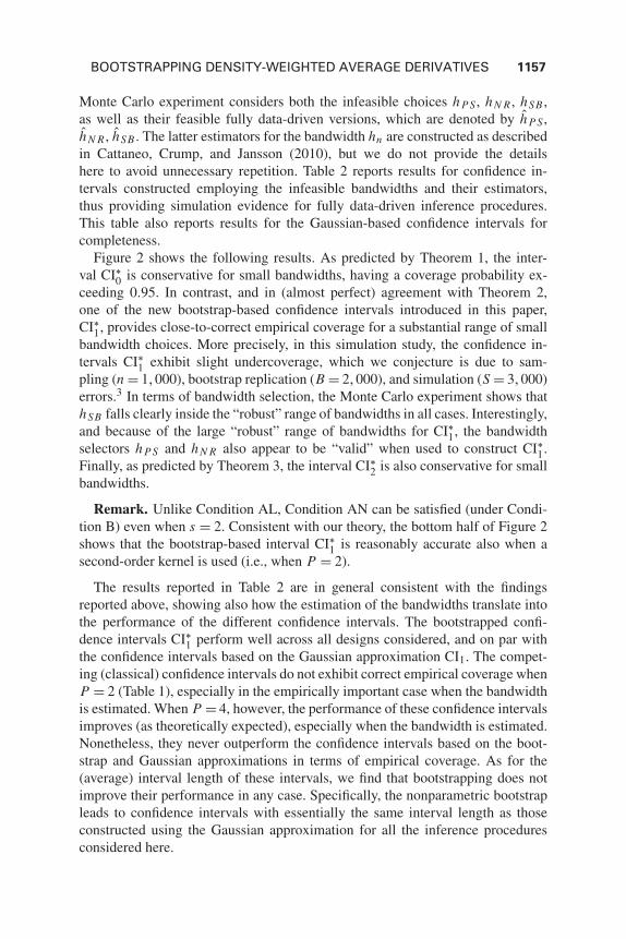
FIGURE 2. Empirical coverage of 95% bootstrap confidence intervals.

and for intervals constructed using estimated bandwidths (further discussedbelow), where c∗

k,α denotes the αth percentile of the distribution of λ′(θ∗n −

nθn/(n −1))/√

λ′V ∗k,nλ for k ∈ {0,1,2}.

The main results from the simulation study are reported in Figure 2 and Table 2.As before, the figure includes the infeasible bandwidth choices h P S and hN R , butnow we also include a third infeasible bandwidth choice, denoted hSB , whichis compatible with the small bandwidth asymptotic framework. These are themain “optimal” bandwidth choices available in the literature for θn(hn) and takethe form

h P S = CP S n− 22s+d+2 , hN R = CN R n− 2

2s+d+2 , hSB = CSB n− 22s+d ,

where CP S , CN R , and CSB are fixed constants depending on the populationparameter of interest and the underlying data generating process. The exact formof these constants, as well as a detailed discussion and comparison of thesebandwidth selectors, is available in Cattaneo, Crump, and Jansson (2010). The

BOOTSTRAPPINGDENSITY-WEIGHTEDAVERAGEDERIVATIVES

1155

TABLE 2. Empirical coverage and interval length of 95% confidence intervals

Empirical coverage Empirical coverage Interval length Interval lengthBandwidth (bootstrap approx.) (Gaussian approx.) (bootstrap approx.) (Gaussian approx.)

hn CI∗0 CI∗0,BC CI∗1 CI0 CI0,BC CI1 CI∗0 CI∗0,BC CI∗1 CI0 CI0,BC CI1

Model 1P = 2 h P S 0.205 0.930 0.809 0.917 0.942 0.825 0.902 0.013 0.013 0.013 0.014 0.014 0.013

hN R 0.205 0.930 0.809 0.917 0.942 0.825 0.902 0.013 0.013 0.013 0.014 0.014 0.013hSB 0.092 0.976 0.843 0.944 0.994 0.897 0.942 0.041 0.041 0.034 0.047 0.047 0.034

h P S 0.209 0.874 0.764 0.855 0.890 0.786 0.845 0.014 0.014 0.014 0.016 0.016 0.014hN R 0.209 0.874 0.764 0.855 0.890 0.786 0.845 0.014 0.014 0.014 0.016 0.016 0.014hSB 0.088 0.973 0.837 0.942 0.987 0.890 0.948 0.071 0.071 0.058 0.083 0.083 0.059

Model 1P = 4 h P S 0.417 0.951 0.952 0.949 0.956 0.951 0.944 0.012 0.012 0.012 0.012 0.012 0.012

hN R 0.442 0.950 0.943 0.949 0.952 0.935 0.941 0.012 0.012 0.012 0.012 0.012 0.012hSB 0.284 0.956 0.983 0.953 0.975 0.991 0.947 0.015 0.015 0.014 0.016 0.016 0.014

h P S 0.242 0.961 0.987 0.917 0.975 0.993 0.926 0.019 0.019 0.017 0.021 0.021 0.017hN R 0.257 0.956 0.986 0.918 0.970 0.991 0.926 0.018 0.018 0.016 0.020 0.020 0.016hSB 0.148 0.983 0.999 0.946 0.996 1.000 0.954 0.045 0.045 0.037 0.052 0.052 0.038

Table continues on overleaf

1156MATIASD.CATTANEOETAL.

TABLE 2. continued

Empirical coverage Empirical coverage Interval length Interval lengthBandwidth (bootstrap approx.) (Gaussian approx.) (bootstrap approx.) (Gaussian approx.)

hn CI∗0 CI∗0,BC CI∗1 CI0 CI0,BC CI1 CI∗0 CI∗0,BC CI∗1 CI0 CI0,BC CI1

Model 2P = 2 h P S 0.157 0.948 0.845 0.930 0.965 0.878 0.928 0.017 0.017 0.016 0.019 0.019 0.016

hN R 0.157 0.948 0.845 0.930 0.965 0.878 0.928 0.017 0.017 0.016 0.019 0.019 0.016hSB 0.055 0.981 0.826 0.947 0.995 0.881 0.957 0.105 0.105 0.086 0.123 0.123 0.087

h P S 0.172 0.902 0.796 0.875 0.921 0.822 0.875 0.018 0.018 0.017 0.020 0.020 0.017hN R 0.172 0.902 0.796 0.875 0.921 0.822 0.875 0.018 0.018 0.017 0.020 0.020 0.017hSB 0.075 0.983 0.839 0.955 0.992 0.887 0.961 0.093 0.093 0.077 0.109 0.109 0.078

Model 2P = 4 h P S 0.314 0.946 0.954 0.938 0.958 0.963 0.940 0.015 0.015 0.014 0.016 0.016 0.014

hN R 0.333 0.943 0.945 0.938 0.955 0.954 0.937 0.014 0.014 0.014 0.015 0.015 0.014hSB 0.183 0.971 0.997 0.952 0.987 1.000 0.947 0.026 0.026 0.023 0.030 0.030 0.023

h P S 0.197 0.965 0.986 0.920 0.979 0.991 0.928 0.025 0.025 0.022 0.029 0.029 0.023hN R 0.209 0.962 0.984 0.918 0.976 0.989 0.923 0.023 0.023 0.021 0.027 0.027 0.021hSB 0.124 0.976 0.996 0.945 0.992 0.998 0.951 0.061 0.061 0.051 0.071 0.071 0.051

Notes:(i) “Empirical Coverage” columns report average coverage rate for each confidence interval.(ii) “Interval Length” columns report average interval length for each confidence interval.(iii) “Bandwidth” columns report either population “optimal” bandwidth or average of estimated bandwidths.


Monte Carlo experiment considers both the infeasible choices h P S , hN R , hSB ,as well as their feasible fully data-driven versions, which are denoted by h P S ,hN R , hSB . The latter estimators for the bandwidth hn are constructed as describedin Cattaneo, Crump, and Jansson (2010), but we do not provide the detailshere to avoid unnecessary repetition. Table 2 reports results for confidence in-tervals constructed employing the infeasible bandwidths and their estimators,thus providing simulation evidence for fully data-driven inference procedures.This table also reports results for the Gaussian-based confidence intervals forcompleteness.

Figure 2 shows the following results. As predicted by Theorem 1, the inter-val CI∗0 is conservative for small bandwidths, having a coverage probability ex-ceeding 0.95. In contrast, and in (almost perfect) agreement with Theorem 2,one of the new bootstrap-based confidence intervals introduced in this paper,CI∗1, provides close-to-correct empirical coverage for a substantial range of smallbandwidth choices. More precisely, in this simulation study, the confidence in-tervals CI∗1 exhibit slight undercoverage, which we conjecture is due to sam-pling (n = 1,000), bootstrap replication (B = 2,000), and simulation (S = 3,000)errors.3 In terms of bandwidth selection, the Monte Carlo experiment shows thathSB falls clearly inside the “robust” range of bandwidths in all cases. Interestingly,and because of the large “robust” range of bandwidths for CI∗1, the bandwidthselectors h P S and hN R also appear to be “valid” when used to construct CI∗1.Finally, as predicted by Theorem 3, the interval CI∗2 is also conservative for smallbandwidths.

Remark. Unlike Condition AL, Condition AN can be satisfied (under Condi-tion B) even when s = 2. Consistent with our theory, the bottom half of Figure 2shows that the bootstrap-based interval CI∗1 is reasonably accurate also when asecond-order kernel is used (i.e., when P = 2).

The results reported in Table 2 are in general consistent with the findingsreported above, showing also how the estimation of the bandwidths translate intothe performance of the different confidence intervals. The bootstrapped confi-dence intervals CI∗1 perform well across all designs considered, and on par withthe confidence intervals based on the Gaussian approximation CI1. The compet-ing (classical) confidence intervals do not exhibit correct empirical coverage whenP = 2 (Table 1), especially in the empirically important case when the bandwidthis estimated. When P = 4, however, the performance of these confidence intervalsimproves (as theoretically expected), especially when the bandwidth is estimated.Nonetheless, they never outperform the confidence intervals based on the boot-strap and Gaussian approximations in terms of empirical coverage. As for the(average) interval length of these intervals, we find that bootstrapping does notimprove their performance in any case. Specifically, the nonparametric bootstrapleads to confidence intervals with essentially the same interval length as thoseconstructed using the Gaussian approximation for all the inference proceduresconsidered here.


5. CONCLUSION

Using an alternative asymptotic framework that removes the bandwidth condi-tions implying asymptotic linearity, we obtained new theory-based predictionsabout the finite-sample behavior of a variety of bootstrap-based inference proce-dures associated with the density-weighted averaged derivative estimator of PSS.In important respects, the predictions and methodological prescriptions emergingfrom the analysis presented here differ from those obtained by NR, who employedtraditional bandwidth conditions and Edgeworth expansions.

The main qualitative findings obtained herein for the density-weighted aver-age derivative estimator of PSS should extend to other kernel-based statisticsthat are asymptotically equivalent to n-varying second-order U -statistics when“small” bandwidths are also employed. Examples of statistics having the lat-ter property include density-weighted averages (see Newey, Hsieh, and Robins,2004, Section 2, and references therein), certain functionals of U-processes (seeAradillas-Lopez, Honore, and Powell, 2007 and references therein), and kernel-based specification test statistics (see Li and Racine, 2007, Ch. 12 and referencestherein). However, and perhaps surprisingly, in recent work (Cattaneo, Crump,and Jansson, 2013) we found that our results are not applicable to kernel-based(nondensity-)weighted average derivative estimators, as these estimators are notasymptotically equivalent to n-varying second-order U-statistics when smaller-than-usual bandwidths are employed.

NOTES

1. For reviews, see, e.g., Politis, Romano, and Wolf (1999) and Horowitz (2001).2. The discussion below also applies immediately to the centered version of Efron-type confidence

intervals, usually known as the “percentile method”.3. We did not explore further this point because of computational limitations.

REFERENCES

Aradillas-Lopez, A., B.E. Honore, & J.L. Powell (2007) Pairwise difference estimation with nonpara-metric control variables. International Economic Review 48, 1119–1158.

Bickel, P.J. & D.A. Freedman (1981) Some asymptotic theory for the bootstrap. Annals of Statistics9(6), 1196–1217.

Cattaneo, M.D., R.K. Crump, & M. Jansson (2010) Robust data-driven inference for density-weightedaverage derivatives. Journal of the American Statistical Association 105(491), 1070–1083.

Cattaneo, M.D., R.K. Crump, & M. Jansson (2014) Small bandwidth asymptotics for density-weightedaverage derivatives. Econometric Theory 30(1), 176–200.

Cattaneo, M.D., R.K. Crump, & M. Jansson (2013) Generalized jackknife estimators of weightedaverage derivatives (with comments and rejoinder). Journal of the American Statistical Association108(504), 1243–1268.

Chen, X., O. Linton, & I. van Keilegom (2003) Estimation of semiparametric models when the crite-rion function is not smooth. Econometrica 71(5), 1591–1608.

Cheng, G. & J.Z. Huang (2010) Bootstrap consistency for general semiparametric M-estimation.Annals of Statistics 38(5), 2884–2915.


Efron, B. & C. Stein (1981) The jackknife estimate of variance. Annals of Statistics 9(3), 586–596.Gine, E. & J. Zinn (1990) Bootstrapping general empirical measures. Annals of Probability 18(2),

851–869.Hall, P. (1992) The Bootstrap and Edgeworth Expansions. Springer.Hardle, W. & A. Tsybakov (1993) How sensitive are average derivatives? Journal of Econometrics

58, 31–48.Heyde, C.C. & B.M. Brown (1970) On the departure from normality of a certain class of martingales.

Annals of Mathematical Statistics 41(6), 2161–2165.Horowitz, J. (2001) The bootstrap. In J. Heckman & E. Leamer (eds.), Handbook of Econometrics,

vol. V, pp. 3159–3228. Elsevier Science B.V.Li, Q. & S. Racine (2007) Nonparametric Econometrics. Princeton University Press.Newey, W.K., F. Hsieh, & J.M. Robins (2004) Twicing kernels and a small bias property of semipara-

metric estimators. Econometrica 72, 947–962.Nishiyama, Y. & P.M. Robinson (2000) Edgeworth expansions for semiparametric averaged deriva-

tives. Econometrica 68(4), 931–979.Nishiyama, Y. & P.M. Robinson (2001) Studentization in Edgeworth expansions for estimates of semi-

parametric index models. In C. Hsiao, K. Morimune, & J.L. Powell (eds.), Nonlinear StatisticalModeling: Essays in Honor of Takeshi Amemiya, pp. 197–240. Cambridge University Press.

Nishiyama, Y. & P.M. Robinson (2005) The bootstrap and the Edgeworth correction for semiparamet-ric averaged derivatives. Econometrica 73(3), 197–240.

Politis, D. & J. Romano (1994) Large sample confidence regions based on subsamples under minimalassumptions. Annals of Statistics 22(4), 2031–2050.

Politis, D., J. Romano, & M. Wolf (1999) Subsampling. Springer.Powell, J.L., J.H. Stock, & T.M. Stoker (1989) Semiparametric estimation of index coefficients.

Econometrica 57(6), 1403–1430.Powell, J.L. & T.M. Stoker (1996) Optimal bandwidth choice for density-weighted averages. Journal

of Econometrics 75(2), 291–316.Robinson, P.M. (1995) The normal approximation for semiparametric averaged derivatives. Econo-

metrica 63, 667–680.Stoker, T.M. (1986) Consistent estimation of scaled coefficients. Econometrica 54(6), 1461–1481.Xiong, S. & G. Li (2008) Some results on the convergence of conditional distributions. Statistics and

Probability Letters 78(18), 3249–3253.

APPENDIX

Auxiliary Lemmas. For λ ∈ Rd , let Ui j,n (λ) = λ′[U (zi , zj ; hn)− θ(hn)]

and define

T1,n(λ) =(

n

2

)−1 ∑1≤i< j≤n

Ui j,n(λ), T2,n(λ) =(

n

2

)−1 ∑1≤i< j≤n

Ui j,n(λ)2,

T3,n(λ) =(

n

3

)−1 ∑1≤i< j<k≤n

Ui j,n(λ)Uik,n(λ)+ Ui j,n(λ)Ujk,n(λ)+ Uik,n(λ)Ujk,n(λ)

3,

T4,n(λ) =(

n

4

)−1 ∑1≤i< j<k<l≤n

Ui j,n(λ)Ukl,n(λ)+ Uik,n(λ)Ujl,n(λ)+ Uil,n(λ)Ujk,n(λ)

3,


as well as their bootstrap analogs

T ∗1,n(λ) =

(m

2

)−1 ∑1≤i< j≤m

U∗i j,n(λ), T ∗

2,n(λ) =(

m

2

)−1 ∑1≤i< j≤m

U∗i j,n(λ)2,

T ∗3,n(λ) =

(m

3

)−1 ∑1≤i< j<k≤m

U∗i j,n(λ)U∗

ik,n(λ)+ U∗i j,n(λ)U∗

jk,n(λ)+ U∗ik,n(λ)U∗

jk,n(λ)

3,

T ∗4,n(λ) =

(m

4

)−1 ∑1≤i< j<k<l≤m

U∗i j,n(λ)U∗

kl,n(λ)+ U∗ik,n(λ)U∗

jl,n(λ)+ U∗il,n(λ)U∗

jk,n(λ)

3,

where U∗i j,n(λ) = λ′[U (z∗

i , z∗j ; hm)− θ∗ (hm)

].

The proof of Lemma 2 uses four technical lemmas, proofs of which are provided in thesupplemental appendix. Lemma A.1 relates �n and �n (and their bootstrap analogs) toT1,n, T2,n, T3,n, and T4,n (and their bootstrap analogs), Lemma A.2 gives some asymp-totic properties of T1,n, T2,n, T3,n, and T4,n (and their bootstrap analogs), while LemmasA.3 and A.4 are used to establish a pointwise version of (4) and to deduce (4) from its

pointwise counterpart, respectively. Let ηn = 1/min(

1,nhd+2n

).

LEMMA A.1. If the assumptions of Lemma 2 hold and if λ ∈ Rd , then

(a) λ′�n(hn)λ = 4[1+o(1)]n−1T2,n(λ)+4[1+o(1)]T3,n(λ)−4T1,n(λ)2,

(b) h−(d+2)n λ′�n(hn)λ = [1 + o(1)]T2,n(λ)− T1,n(λ)2 − 2[1 + o(1)]T3,n(λ)+ 2[1 +

o(1)]T4,n(λ),

(c) λ′�∗n (hm)λ = 4[1+o(1)]m−1T ∗

2,n(λ)+4[1+o(1)]T ∗3,n(λ)−4T ∗

1,n(λ)2,

(d) h−(d+2)m λ′�∗

n(hm)λ = [1+o(1)]T ∗2,n(λ)− T ∗

1,n(λ)2 −2[1+o (1)]T ∗3,n(λ)+2[1+

o(1)]T ∗4,n(λ).


(a) T1,n(λ) = op(√

ηn),

(b) T2,n(λ) = E[Ui j,n(λ)2]+op(h−(d+2)

n),

(c) T3,n(λ) = E[(E[Ui j,n(λ)|zi ])2]+op(ηn),

(d) T4,n(λ) = op (ηn),

(e) hd+2n E

[Ui j,n(λ)2] → λ′�λ and E

[(E[U i j,n(λ)|zi ])2] → λ′�λ/4,

(f ) T ∗1,n(λ) = op

(√ηm

),

(g) T ∗2,n(λ) = E∗[U∗

i j,n(λ)2]+op(h−(d+2)

m),

(h) T ∗3,n(λ) = E∗[(E∗[U∗

i j,n(λ)|z∗i ])2]+op(ηm),

(i) T ∗4,n(λ) = op(ηm),

(j) hd+2m E

∗[U∗i j,n(λ)2] →p λ′�λ and

E∗[(E∗[U∗

i j,n (λ) |z∗i ])2]−λ′�n(hm)λ/4 →p 0.



(a) E[(E∗[U∗

i j,n(λ)|z∗i ])4] = O

(η2

m +h2mη3

m),

(b) E[U∗

i j,n(λ)4] = O(h−(3d+4)

m),

(c) E[(E∗[U∗

i j,n(λ)2|z∗i ])2] = O

(m−1h−(3d+4)

m +h−(2d+4)m

),

(d) E[(E∗[U∗

i j,n(λ)U∗ik,n(λ)|z∗

j , z∗k ])2] = O

(h−(d+4)

m +m−2h−(3d+4)m

),

(e) E[(E∗[E∗[U∗

i j,n(λ)|z∗i ]U∗

i j,n(λ)|z∗j ])2] = O

(1+m−1h−(d+4)

m +m−3h−(3d+4)m

).

LEMMA A.4. There exist constants C and J (only depending on d) and a collection

l1, . . . , l J ∈ �d such that for every d ×d matrix M, supλ∈�d

(λ′Mλ

)2 ≤ C∑J

j=1(l ′j Mlj

)2.

Proof of Lemma 2. As noted in the discussion of Lemma 2,

V∗ [θ∗

n

]= m−1

V∗ [L∗(z∗

i ; hm)]+(

m

2

)−1V

∗ [W∗(z∗i , z∗

j ; hm)]

,

where, using Lemmas A.1 and A.2,

V∗[L∗(z∗

i ; hm)] =(

n −1

n

)2�n(hm) = � +2

m2

n

(m

2

)−1h−(d+2)

m �+op (ηm) .

The proof of part (a) can be completed by using Lemmas A.1 and A.2 to show that

λ′V

∗[W∗(z∗i , z∗

j ; hm)]λ = h−(d+2)m

(n −1

n

)[λ′�n(hm)λ+op (1)

]

− 3

2

(n −1

n

)2λ′�n(hm)λ

= h−(d+2)m λ′�λ+op (mηm)

(∀λ ∈ Rd

).

Next, part (b) can be established by using Lemmas A.1 and A.2 to show that

λ′�∗n (hm)λ = 4[1+o (1)]m−1T ∗

2,n(λ)+4[1+o (1)]T ∗3,n(λ)−4T ∗

1,n(λ)2

= λ′�n(hm)λ+4m−1h−(d+2)m λ′�λ+op(ηm)

= λ′�∗nλ+op (ηm)

(∀λ ∈ Rd

).

Finally, to establish part (c), the theorem of Heyde and Brown (1970) is employed toprove the following condition, which is equivalent to (4) in view of part (a):

supλ∈�d

supt∈Rd

∣∣∣∣P∗[λ′(θ∗

n − θ∗n )/

√λ′V∗[θ∗

n ]λ ≤ t

]− 1 (t)

∣∣∣∣ →p 0.

For any λ ∈ �d ,

λ′ (θ∗n − θ∗

n

)/

√λ′V∗[θ∗

n ]λ =∑

1≤i≤m

Y ∗i,m (λ) ,


where, defining L∗i,m(λ) = λ′L∗(z∗

i ; hm)

and W∗i j,m(λ) = λ′W∗(z∗

j , z∗i ; hm

),

Y ∗i,m(λ) =

⎡⎣m−1L∗

i,m(λ)+∑

1≤ j<i

(m

2

)−1W∗

i j,m(λ)

⎤⎦/

√λ′V∗[θ∗

n ]λ.

For any n,(Y ∗

i,m(λ),F∗i,n

)is a martingale difference sequence, where F∗

i,n =σ(Zn, z∗

1, . . . , z∗i

). Therefore, by the theorem of Heyde and Brown (1970), there exists

a constant C such that

supλ∈�d

supt∈Rd

∣∣∣∣P∗[λ′(θ∗

n − θ∗n )/

√λ′V∗[θ∗

n ]λ ≤ t

]− 1 (t)

∣∣∣∣≤ C sup

λ∈�d

⎧⎪⎨⎪⎩

∑1≤i≤m

E∗ [Y ∗

i,m(λ)4]+E∗

⎡⎢⎣⎛⎝ ∑

1≤i≤m

E

[Y ∗

i,m(λ)2∣∣∣F∗

i−1,n

]−1

⎞⎠2

⎤⎥⎦⎫⎪⎬⎪⎭

1/5

.

Moreover, by Lemma A.4,

supλ∈�d

⎧⎪⎨⎪⎩

∑1≤i≤m

E∗ [Y ∗

i,m(λ)4]+E∗

⎡⎢⎣⎛⎝ ∑

1≤i≤m

E

[Y ∗

i,m(λ)2∣∣∣F∗

i−1,n

]−1

⎞⎠2

⎤⎥⎦⎫⎪⎬⎪⎭ →p 0

if (and only if) (A.1)–(A.2) hold for every λ ∈ �d , where∑1≤i≤m

E∗ [Y ∗

i,m(λ)4]

→p 0, (A.1)

E∗⎡⎢⎣⎛⎝ ∑

1≤i≤m

E

[Y ∗

i,m(λ)2∣∣∣F∗

i−1,n

]−1

⎞⎠2

⎤⎥⎦ →p 0. (A.2)

The proof of part (c) will be completed by fixing λ ∈ �d and verifying (A.1)–(A.2) .

First, using(λ′V ∗[θ∗

n ]λ)−1 = Op

(mη−1

m)

and basic inequalities, it can be shown that (A.1)holds if

R1,m = m−2η−2m

∑1≤i≤m

E

[L∗

i,m(λ)4]

→ 0,

R2,m = m−6η−2m

∑1≤i≤m

E

⎡⎢⎣⎛⎝ ∑

1≤ j<i

W∗i j,m(λ)

⎞⎠4

⎤⎥⎦ → 0.

Both conditions are satisfied because, using Lemma A.3,

R1,m = O(

m−1η−2m E[(E∗[U∗

i j,n (λ) |z∗i ])4]

)= O

(m−1 +m−1h2

mηm

)= O

(m−1 +m−2h−d

m

)→ 0


and

R2,m = O(

m−4η−2m E[U∗

i j,n(λ)4]+m−3η−2m E[(E∗[U∗

i j,n(λ)2|z∗i ])2]

)= O

(m−4η−2

m h−(3d+4)m +m−3η−2

m h−(2d+4)m

)= O

(m−2h−d

m +m−1)

→ 0.

Next, consider (A.2). Because

(λ′V

∗[θ∗n ]λ)

⎡⎣ ∑

1≤i≤m

E

[Y ∗

i,m(λ)2∣∣∣F∗

i−1,n

]−1

⎤⎦ =

(m

2

)−2

×∑

1≤i≤m

⎛⎜⎝E

⎡⎢⎣⎛⎝ ∑

1≤ j<i

W∗i j,m(λ)

⎞⎠2

∣∣∣∣∣∣∣F∗i−1,n

⎤⎥⎦−

∑1≤ j<i

E∗ [W∗

i j,m(λ)2]⎞⎟⎠

+2m−1(

m

2

)−1 ∑1≤ j<i≤m

E

[L∗

i,m(λ)W∗i j,m(λ)|F∗

i−1,n

],

it suffices to show that

R3,m = m−6η−2m E

⎡⎢⎣⎛⎝ ∑

1≤ j<i≤m

{E

[W∗

i j,m(λ)2∣∣∣F∗

i−1,n

]E

∗ [W∗i j,m(λ)2

]}⎞⎠2⎤⎥⎦ → 0,

R4,m = m−6η−2m E

⎡⎢⎣⎛⎝ ∑

1≤k< j<i≤m

E

[W∗

i j,m(λ)W∗ik,m(λ)

∣∣∣F∗i−1,n

]⎞⎠2⎤⎥⎦ → 0,

R5,m = m−4η−2m E

⎡⎢⎣⎛⎝ ∑

1≤ j<i≤m

E

[L∗

i,m(λ)W∗i j,m(λ)|Zn, z∗

j

]⎞⎠2⎤⎥⎦ → 0.

By simple calculations and Lemma A.3,

R3,m = O(

m−4η−2m E[W∗

i j,m(λ)4])

= O(

m−4η−2m E[U∗

i j,n(λ)4])

= O(

m−4η−2m h−(3d+4)

m

)= O

(m−2h−d

m

)→ 0,

R4,m = O

(m−2η−2

m E

[(E

∗[W∗i j,m(λ)W∗

ik,m(λ)|z∗j , z∗

k ])2])

= O

(m−2η−2

m E

[(E

∗[U∗i j,n(λ)U∗

ik,n(λ)|z∗j , z∗

k ])2])

= O(

m−2η−2m h−(d+4)

m +m−4η−2m h−(3d+4)

m

)= O

(hd

m +m−2h−dm

)→ 0,


R5,m = O

(m−1η−2

m E

[(E

∗ [L∗i,m(λ)W∗

i j,m(λ)|z∗j

])2])

= O

(m−1η−2

m E

[(E

∗ [E

∗[U∗i j,n(λ)|z∗

i ]U∗i j,n(λ)|z∗

j

])2])

= O(

m−1η−2m +m−2η−2

m h−(d+4)m +m−4η−2

m h−(3d+4)m

)= O

(m−1 +hd

m +m−2hdm

)→ 0,

as was to be shown. n

30 BOOTSTRAPPING DENSITY-WEIGHTED AVERAGE DERIVATIVES€¦ · BOOTSTRAPPING DENSITY-WEIGHTED...

Documents

Transcript of 30 BOOTSTRAPPING DENSITY-WEIGHTED AVERAGE DERIVATIVES€¦ · BOOTSTRAPPING DENSITY-WEIGHTED...