3 TRANSPORTATION SYSTEM INVENTORY - Oregon Procedure Manual Version 2 3-1 Last Updated 09/2017 3...

Analysis Procedure Manual Version 2 3-1 Last Updated 09/2017

3 TRANSPORTATION SYSTEM INVENTORY

3.1 Purpose Before any analysis can begin, data for the study area must be collected from the field or other available in-office sources. This chapter provides guidance in the selection criteria and collection methods of appropriate inventory data types for use in transportation analysis. Inventory data is the foundation that all other later decisions are based on, so it is important that the scope of the data collection is appropriate and adequate to support the needs/outcomes of the plan or project.

3.2 Office Data Resources There is a wide range of data sources that can be obtained prior to the field investigation. Gathering this information gives the analyst a “feel” of the study area and what level of data is available, what may need to be verified versus gathered.

3.2.1 Crash Data Crash data can come from a variety of sources, and is useful for identifying problem areas of the highway experiencing an above-average frequency of crashes or reoccurring crash patterns. The analysis procedures that use this data are described in following chapters, while the data itself is described below. Sources of Crash Data The following describes sources of crash related data and information. Tools available for the analyst to use in crash analysis are discussed in Chapter 4. Oregon Motor Vehicle Traffic Crash Database ODOT’s Crash Analysis and Reporting (CAR) Unit provides the official motor vehicle crash data through database creation, maintenance and quality assurance, information and reports and limited database access. Crash data since 1985 is maintained at all times. Vehicle crashes include those coded for city streets, county roads and state highways. The CAR Unit website offers a variety of publications containing information on monthly and annual crash summaries. Although there are other sources of information, such as police departments, local groups that collect information, and anecdotal information, the ODOT CAR Unit data is the standard source. Oftentimes these other sources include reporting calls, not the actual investigation/report, and groups often include near-misses and/or don’t have all the facts, so the report is erroneous. The CAR data has the checks and balances built into the data collection that matches “both sides of the reports” for a crash, treating all areas the same so comparisons can be made. This is also the database used to calculate all the comparison rates published in the crash rate books. The CAR Unit obtains documentation of reported crashes from DMV and other sources which they use to code the crash database. It should be noted that not all crashes are reportable, not all


those that should be reported are reported, many of those reportable are filed out by citizens with attendant limitations on data accuracy, and even those law enforcement reported may have issues with accuracy. The documentation provided to the CAR Unit can range from being very thorough to very limited and can include conflicting or incorrect information. The documentation is carefully checked and may be corrected before being coded. Crash codes are defined in the ODOT Traffic Crash Analysis and Code manual, available on the TransData Crash Data webpage. For detailed information about the coding process contact the CAR Unit. Depending on the level of analysis needed, there are various reports that can be obtained. It should be noted that even though this database often represents the most current data available, data for a given year is typically not available until at least 6 months into the following year. Detailed information for individual crashes can also be obtained by contacting the CAR Unit and specifying the segment of highway (roadway) and time period of interest. Because crashes are reported by specific points, an issue may be located just outside of the analysis area. Therefore, the area of requested crash data should always be greater than the area of analysis. The additional distance should be enough to catch the character of the road such as the adjacent blocks in an urban setting and a quarter to half mile in a rural setting. Crash data is always available from the CAR unit and should be obtained through them for complex, controversial or legal situations since they are the official reporting source. For most analysis efforts, using the on-line reports is sufficient. Crash data is available on both state highways and local roads on the ODOT Internal Crash Reports website or the External Crash Reports website. Crash data is requested by state highway number and milepoint for specific years. Local road crashes are available at the above websites by clicking on the Local Roads tab. Crash information is categorized first by county, then city and finally by street name. Selecting the summary detail will bring up the entire length of the roadway. The summary is only useful when the entire roadway in within the study area. If only a portion of the street is desired, the data needs to be obtained from the comprehensive report (PRC). The analyst will need to review the report and select the appropriate crashes to summarize for use in the analysis. While several years of data may be available for any given roadway segment, it is common practice to analyze only the most recent, complete three to five (3-5) years of data as factors such as traffic volumes, environmental conditions and roadway characteristics may change with time. Three years of data gives a minimal picture and is the minimum analysis period for a safety analysis, while the five year listing gives a more desirable view. Roadways with a small number of crashes should be looked at through a five year period to get a better representative sample. In some circumstances even a longer period may be reviewed. Also, remember that the crash databases are regularly updated to include more recent data, so care should be taken to select the correct timeframe(s). For more information on pulling crash data, refer to Appendix 4A. Safety Priority Index System The Safety Priority Index System (SPIS) is a method developed by ODOT in 1986 to flag

https://www.oregon.gov/ODOT/Data/Pages/Crash.aspx


http://highway.intranet.odot.state.or.us/tad/tvc/

https://zigzag.odot.state.or.us/uniquesig2a2763047fdf9d8485a3bef41dc862de/uniquesig0/SecurezigzagAPortalHomePage/


https://www.oregon.gov/ODOT/Planning/Documents/APMv2_App4A.docx


potential safety issues on state highways. Major revisions have occurred from the original process. The SPIS score is based on three years of crash data, and considers crash frequency, crash rate and crash severity. ODOT bases its SPIS on 0.10-mile segments to account for variances in how crash locations are reported. To become a SPIS site, a location must meet one of the following criteria:

• Three or more crashes have occurred at the same location over the previous three years. • One or more fatal crashes have occurred at the same location over the previous three

years. The use of this information is discussed in the Safety Chapter (4) and the documentation on how the SPIS is calculated can be found at the Safety Priority Index System website. Any SPIS listing can be obtained by ODOT staff. Non-ODOT analysts can obtain the SPIS listing by contacting ODOT Region Traffic personnel. Top 5% and 10% sites need to be included in any crash analysis of a study area. SPIS-All Roads (Internal Use Only) The program is a tool internal to ODOT which is a variation of the standard SPIS program. SPIS-All Roads contains crash data for local roads as well as the state highway. It allows the data to be filtered based on specific fields and then have the SPIS calculation reported. TransGIS Mapping Tool TransGIS is a web mapping tool designed for users of every skill level. It presents many data levels in an interactive map format in multi-level views. This mapping tool provides more detailed information on many types of safety, volume and crash data on a state map. The user can choose the information that is displayed, and can zoom into the map to increase detail as well as display city and county maps behind this data. Extensive work with individual layers may be required in the generic TransGIS application, to obtain all necessary information about a study segment. A decoded crash layer is available For external access to the newer TransGIS 2.0 follow the link and click on “New TransGIS 2.0” The ODOT GIS Unit may be able to produce custom maps or applications in some cases, depending on the nature of the request and work priorities. GIS maps or web applications may be possible, as well as additions to TransGIS. A web application is a custom TransGIS website with pre-defined layers. GIS software is not required. The user can zoom in/out and turn layers on/off as desired. The application may be permanent or temporary, as needed for the duration of the project. Examples are located on the GIS Unit Applications Webpage. All requests for mapping products are submitted to the ODOT GIS Unit (GISU) from ODOT staff. Consultants may initiate a request through ODOT staff. Requests should be clearly defined prior to submittal to avoid re-work. Contact the GIS Unit for further information. Custom mapping requests need to use the GIS Project Request form which is available by contacting the GISU.

https://www.oregon.gov/ODOT/Engineering/Pages/SPIS-Reports-On-State.aspx

https://gis.odot.state.or.us/transgis/

http://transnet.odot.state.or.us/tdd/GIS/Shared%20Documents/Applications.aspx


Crash (Collision) Diagrams Crash diagrams are typically used to evaluate operational and safety projects, not analytical ones. The typical project and planning analysis would not require this level of detail. The CAR Unit can create a crash diagram that depicts the crashes on a given roadway section. Depending on the size of area requested and the number of crashes in the requested area, this can be time consuming. For more information, refer to the ODOT Safety Investigation Manual available on the ODOT Highway Safety Manual webpage. Crash Rate Tables Crash Rate Tables have been published annually by the CAR Unit since 1948. Tables in the front of the book list statewide crash rates for several categories of the State Highway System. More tables list the crash rates for selected sections of each state highway, as well as a rural/urban break out. Additional tables list intersection crash data and fatal crash data. These tables are discussed further in the Safety chapter and are available on the Crash Statistics and Reports webpage.

3.2.2 Roadway Data ODOT maintains a wide variety of roadway characteristic and features data available on the ODOT State Highway Reports. TransGIS including the newer TransGIS 2.0 is available on the ODOT Internal TransGIS website or the External TransGIS website. These sites are also available on the Consultant Portal under the Data and Reports section on the ODOT Internet site. This data includes and is not limited to: Roadway alignment – horizontal and vertical (grades) Roadway cross-sectional data – lane, shoulder and median widths Roadway features – pavement type, number of lanes, speed limits Roadway details – structures, connections, mile points and equations Segment Vehicle Classifications and Characteristics Summarized Traffic Information Other data sources are also available through the above links. They include: Digital Video log Traffic Count Information Functional Classifications Highway Classifications including freight routes, scenic byways Operations and Performance Standards including spacing and mobility Design Standards ODOT generated maps Additional Data that should be located includes:

https://www.oregon.gov/ODOT/Engineering/Pages/HSM.aspx



https://www.oregon.gov/ODOT/Data/Pages/Road-Assets-Mileage.aspx#reports

http://gisintra.odot.state.or.us/TransGIS/

http://gisintra.odot.state.or.us/TransGIS/


http://www.odot.state.or.us/ffp/hwy/opd/consultant.html


Transit Information The following information is likely needed from the local transit authority Transit vehicle characteristics Route specifics such as paths, schedules, dwell time, headway Passenger boarding/alighting and occupancy data Transit specific control and timings Traffic Signal Timing Sheets Traffic signal timing sheets are needed when creating analysis files. The best source of current information for state highways is through the Region Traffic Engineer. Occasionally, the local jurisdiction will be responsible for the signal timing, so they are the source of that data along with any local signalized intersections of interest. Traffic Plan Sheets (If available) An analyst should obtain information related of the roadway and traffic control for the intersections of interest. Specific details such as the detector layouts and striping sheets are available for many areas. Digital PDF copies of signing, striping and signal plans are available at the FileNet Workplace website. This file sharing site is searchable. You can obtain this information by logging in as a guest. Other useful information Information such as zoning and local classification maps needs to come from local jurisdictions. Private entities may have aerial photos also available. Although on-line data sources such as NAVTEQ, Google and Bing may yield useful (scalable) information, they can also contain information that is not very current and may not be consistent between overhead and street/driver views. Street names often differ from the official names. Information from these sources needs to be verified.

3.2.3 Reports and Tools Transportation Planning On-line Database (TPOD) This is a map-based, graphical tool for locating planning studies within a specific area. This may include but is not limited to Transportation System Plans (TSP), refinement plans, Interchange Area Management Plans (IAMP) and others that may have factors that significantly impact the study. For example, a TSP may include alternative mobility standards, local jurisdiction’s operational standards, fiscally constrained project list and many more. Because this tool is only updated periodically, the most recent reports likely are not included in the data. Contact the region planning manager to verify. Features Attributes and Conditions – Statewide Transportation Improvement Program

http://filenet/Workplace/

https://gisprod.odot.state.or.us/tpod/

http://208.109.223.100/facs-stip/home.aspx


(FACS-STIP) This is an ODOT Asset Management database in both listing and map-based forms. Information includes data such as sidewalks, bike facilities, ADA facilities, access locations, and some traffic features. This is an evolving database that is being continually expanded as data is collected. In addition to gathering data from TPOD and other on-line databases, the analyst should determine / locate other studies that may have bearing within the study area, including previous (related) studies, Safety Investigations, and Traffic Impact Studies. The analyst should contact local jurisdictions, the Region Traffic Manager, the Region Access Management Engineer (RAME) and the Region Planning Manager to locate any of this work.

3.3 Field Inventory Specific data related to field conditions that may affect traffic safety and operations shall be collected directly during a visit to the area. In addition, inventory data collected through other sources such as previously conducted studies or databases maintained by the road authority should be field verified. There is no substitute for a field visit as an analyst cannot get a good feel for the project area otherwise. This is a check of other data sources (such as aerial photos) for accuracy. Notes, photographs and/or video should be taken of the project area in addition to the inventory data to reference, and possibly include, as graphical elements in the final report. The most common types of field data needed are discussed below.

3.3.1 Geometric Data Geometric data is the physical characteristics of the facility, typically including:

• Street names • Segment lengths • Lane/shoulder/median widths • Lane configurations • Storage bay and ramp taper lengths • Acceleration and Deceleration lane lengths and tapers • Storage bay lengths (from stop-bar to start of taper) • Bike/multi-use facility locations and dimension • Parking locations and dimensions • Raised medians/pedestrian refuges/islands locations and dimensions • Location of stop/yield bar, intersection guidelines (dashes) • Pedestrian facilities (type, condition, location) including crosswalks dimensions (length

and width) • Intersection and access spacing • Access type, location, width and land use served

3.3.2 Operational Data Operational data describes the characteristics of traffic control and flow, and typically includes:

• Speed limits

http://208.109.223.100/facs-stip/home.aspx


• Saturation flow, speed and travel time studies • Intersection controls (signalized, stop-controlled, yield, merge, etc.) • Signal characteristics (timed, actuated, split-phased, protected left turns, etc.) • Signing (especially turn prohibitions) • Parking signing, striping, and maneuver frequency • Pedestrian crossings including at crosswalks and improper (jay-walking) frequency of

use • Transit stop locations and amenities • Rail crossing locations, train frequency and duration of blockages • Intersection sight distance

3.3.3 Field Observation Data Observations related to travel patterns and driver behavior. This can include:

• Perceived or actual operational problems • Length and duration of queues • Driver behavior for lane choice, turn paths, upstream and downstream movements or

maneuvers, left turn “sneaker” (left turn drivers that turn enter and depart the intersection during the yellow or red intervals)

• Pedestrian, Bicycle or other user behavior including actual travel paths • Evidence of crashes such as glass on the shoulder, tire marks on curbs or medians • Tire wear on pavements • Damaged or worn physical features

3.3.4 Simulation-Specific Data In addition to the geometric and operational field data, additional simulation specific data is needed if a project requires simulation. Simulation-specific data typically may include:

• Number of detectors, length, and distances from stop bar or crosswalk • Turning speeds and radii (if unusual geometrics or conditions exist) • Free-Flow speeds on ramps, highway segments, or on intersection discharge legs

approaches (can be collected using road tubes or speed guns) • Floating car travel times and average speeds • Important travel patterns (OD Data), Example: ~75% of traffic exiting the mall makes

left at Main Street • Lane Use

o Details of user specific lanes (e.g. HOV, truck/bike/bus) o Use of the shoulder or median to move around blockage points or due to driver

confusion/disregard o Lane-change positioning lengths or landmarks where vehicles tend to position

themselves in a lane to make an upcoming turn or merge o Freeway/arterial guide sign locations (for lane change distances) o Noticeable lane imbalance issues (some lanes used more heavily than others) and

causes (i.e. lane drops, multiple turn lanes, closely spaced intersections/accesses,


etc.) o If more than one lane is available to turn into from an approach, indicate the lane

that turning vehicles align into (left or right alignment) regardless if the movement is legally proper or not.

• List the approximate average and maximum queues for each lane • If upstream intersections or bays are blocked by congestion from the observed

intersection, what percentage of the site visit hour did blocking occur <5%, 10%, 25%, 50%?

• Arrival type for each approach (i.e. are the vehicles arriving in a platoon, if so, are they arriving on red or green?)

3.3.5 Safety-Specific Data Additional data beyond the general geometric, operational, and observation data may be needed to support Highway Safety Manual techniques (See Section 4.4.4). Safety-specific data may include:

• Fixed object density and average distance offsets • Intersection skew angle • Presence/absence of centerline rumble strips, lighting, red-light cameras, and automatic

speed enforcement • Number of schools, bus stops and alcohol-selling establishments within 1000’ of an

intersection.

3.3.6 Field Data Collection Requirements For studies not needing simulation, the field inventory data is recommended as it can help the analysis. For projects requiring simulation, the simulation specific field data and counts MUST be collected at a time representing the analysis time period (the 30th highest hour) as closely as possible. The simulation calibration data should be obtained by the analyst conducting/ overseeing the simulation work. This effort should occur during the vehicle count collection if feasible. See the Simulation Chapter for guidance and instruction on calibrating simulations. With some project areas, it is impractical to obtain all counts and inventory on a single day representing the 30th highest hour. When this happens, the counts and field inventory at the primary locations should be on days that closely represent the 30th highest hour. If it is not possible, then short sample counts should occur during the field inventory collection to factor the off-peak counts to the day the study area was visited. Factor the counts for seasonal influences (described in Chapter 5). If this is the case and simulation is required for the study, use the seasonal factor methodology to determine if the vehicle count day is representative of the 30th highest hour. If the study’s primary counts occurred at a time that is more than 10% different than the 30th highest hour period (considering seasonal trend type) then short duration sample counts need to occur during the field collection time to calibrate the “existing conditions” model. The counts need to be at critical locations (high volumes, bottlenecks, unusual conditions) to assist with


representing the traffic flows. These rules are established to help ensure that calibration volumes 1) are near the 30th highest hour and 2) represent conditions that have been witnessed in the field.

3.3.7 Field Inventory Worksheet The Field Inventory Worksheet has been designed by the Transportation Planning Analysis Unit (TPAU) to be generic enough to aid in the collection of field data for all studies. The Field Inventory Worksheet, Exhibit 3-1, assists the field data collection process. The worksheet is an example of how to organize/document the information. It shows much of the suggested information, but it should be customized according the study’s needs. The worksheet can be used for projects where just geometry and observational data is required or for projects requiring simulation where all the data listed above should be addressed. Exhibit 3-1 shows a completed worksheet for a simulation project. Note that the worksheet may be printed multiple times for a given project area. The collection of worksheets can be placed in a three-ring binder providing a hard writing surface. A worksheet can be used for each intersection or area of interest in the study and all copies can be neatly organized in a single project binder. Exhibit 3-1 Field Inventory Worksheet - Intended Setup

https://www.oregon.gov/ODOT/Planning/Documents/APMv2_App3A.pdf



Exhibit 3-2 Completed Example Field Inventory Worksheet

3.4 Vehicle Count Surveys The data collected from vehicle count surveys is used in nearly all types of analysis procedures, and can include information regarding volumes of vehicles, types of vehicles, vehicle speeds and


directions of vehicle flow. When such information is needed, the analyst must determine the appropriate time and method of data collection to obtain the desired results. How many counts of what type is dependent on the context of the plan or project goals and objectives. For outsourced projects and plans, a draft scope/work plan with a completed objective section is critical for efficient use of time, money and data for all involved parties. The level of count detail required will be dictated by the level of detail in the plan or project. For example, Transportation System Plans (TSP) will be less detailed than a TSP Refinement Plan.

3.4.1 Vehicle Count Types and Durations Intersection Classification Counts Intersection classification counts provide vital information for project development. They provide peak hourly volumes (PHV), Average Daily Traffic (ADT) and vehicle classifications such as cars, pickups, buses and trucks for each approach and movement. Additionally, the K-factor (percent of ADT in the peak hour) and the D-factor (percent of traffic in a single direction) can be derived from the intersection count data. These are then used to convert PHV to ADT. For further explanation of traffic volume characteristics, refer to the HCM – Part I: Overview. Intersection classification counts are typically 16-hours in duration, so average daily traffic (ADT) and other relationships can be created. These counts are used at signalized intersections, intersections that may become signalized, and other important major intersections, such as interchange ramp terminals. A 16-hour count is needed when requirements exist such as multiple peak periods, truck classifications, signal warrants, pavement design, air quality and/or noise studies in environmental documents. Sixteen–hour counts can also be easily used for other purposes such as pavement design (see Chapter 6) or other plans or projects. The average cost of an ODOT-performed 16-hour Full Federal Manual Classification Count is approximately $1,100(2012 costs). This cost is dependent on the complexity of the intersection, whether or not it’s a high-volume intersection, and other special requirements including travel. Intersection classification counts group 13 different types of vehicles, pedestrians and bicycles. Refer to the FHWA vehicle classification descriptions in Chapter 6 and in the Environmental Traffic Data Chapter. Classification counts can either be done manually in the field or by use of video cameras. ODOT typically uses video cameras as it does not require the presence of a field technician throughout the duration of the count, may have less influence on driver behavior in some situations, allows for more flexibility in scheduling and processing counts, and provides a database that can be easily revisited if more information is desired at a later time or if an error in the count is detected. Data is recorded in the field and is then sent to the Transportation Systems Monitoring (TSM) Unit for processing. Passenger and other two-axle vehicles are tabulated both with and without trailers. The number of axles for single-unit trucks and for all single, double and triple trailer trucks is recorded along with buses and motorcycles. A number will be given to each count so that it can be accessed easily. A hardcopy will be stored in TSM’s files. Counts are sent to the requestor either electronically as a spreadsheet file or


Peak period counts should not be used to create daily traffic volumes (ADT) in most cases. Exceptions would be volumes to support HSM analyses and preliminary signal warrants where sufficient 12+ hour counts are available to calculate K-factors to be applied to the peak period counts. Air/noise traffic data production must use longer duration counts. See Chapter 5 for more information.

hardcopy by mail. The first page of the ODOT intersection count provides a sketch of the intersection counted, the date, location, count number and the ADT for each movement. The second page provides a summary of movements broken down into 1-hour increments. Some intersection counts will break the peak periods into 15-minute intervals instead of 1-hour intervals. Specify 15-minute count intervals for any period when peak hour factors are needed. The rest of the pages show individual turning movements with the vehicle classifications, a summary of the bicycle and pedestrian counts (if originally requested) and a summary of the movement volumes. Sample Count Request and Sample ODOT Counts have been included in Appendix 3B. Peak Period Counts Peak period counts capture the individual vehicle movements at a location. These counts are typically used to capture the in/out turning movements at driveway accesses or to count all movements at minor or unsignalized intersections that are not being considered for signalization. Generally, separate truck percentages are not available. Use of turning movement counts are limited to counting in a single peak period. Typical peak periods are morning (6:00 AM – 9:00 AM), mid-day (11:00 AM – 1:00 PM), and evening (3:00 PM – 6:00 PM). A three-hour count is a typical duration to capture the peak hour. A four-hour afternoon peak period count can be obtained to capture both school and commuter peaks. Truck peak hours could be any hour outside of the typical commuter peaks so are unlikely to be captured by a peak period count. For count durations of more than four hours or when more than one peak period is needed, it is more practical to collect a 16-hour count. Count durations less than three hours make it difficult to capture the peak hour and should be avoided unless previous counts clearly identify the system peak hour in which case shorter duration counts may be acceptable. Typical ODOT count costs are variable depending on travel, duration, and other specifics, but are in the $600(2012 costs) range.

Road Tube Counts Road tube counts are often employed when the details provided by intersection counts are not needed, impractical given the data needs, when certain additional data is needed that would best be collected by tubes, such as roadway speed (Section 3.5.2), or available gaps in traffic. These count individual vehicles only or can be setup to capture vehicle classifications. These counts are used to capture mid-block volumes on streets and for segment volumes on most highways and interchange ramps. Road tubes are subject to vandalism or damage, and should not be done where vehicles may stop on the tube (in congested areas or near intersections) or cross the tube at an angle (near intersections or driveways) because under or over-counting may occur. Tubes are also susceptible to be damaged on roadways with speeds at or above 40 mph, and for employee safety reasons, cannot be placed on high-volume expressways and freeways. It is also not recommended to use road tubes during winter months (November 1st – April 1st), due to the use

https://www.oregon.gov/ODOT/Planning/Documents/APMv2_App3B.pdf


of studded tires, which have been shown to destroy hose tubes, even at slower city speeds. Road tube counts are typically done in a 48-hour format so an entire 24-hour period can be obtained. A 7-day count can also be done if daily fluctuations over a week are necessary to be captured and are only done on roadway segments. Typical ODOT road tube count costs are around $200(2012

costs).

3.4.2 Other Sources of Traffic Data Information Frequently, existing or alternative count sources are overlooked so these should be reviewed before completing the initial count list. This can, in some cases, substantially reduce the number of new counts, save on data collection costs, and cut down the number of SOW review iterations. When searching for older traffic counts, generally the counts should only be a few years old (3-5). The longer period may be acceptable when there is little to no change in volumes or when developing a preliminary analysis. When counts are older than three years, growth rates may not reflect the growth when much change is occurring. The further the count is being interpolated, the more likely for error to be introduced. See Chapter 6 for information on forecasting. Transportation System Monitoring (TSM) Unit Data

• Previously Collected Counts

Besides obtaining new counts there are some other sources of count information which may be used to reduce the overall new count requirement needs. ODOT has a large quantity of traffic volume data and previously collected counts. Before any new counts are ordered, the Transportation System Monitoring (TSM) Unit should be contacted to determine if any previous usable counts are available for the study area. In general, counts in the study area should be three years old or less. Older counts between three and five years old can sometimes be used if they are the correct type and no significant changes, such as new roads or developments, have occurred to influence traffic flows. A newer count may not accurately represent the traffic flows on a roadway section even if less than the three years old if recent development has occurred within or near the study area since the count was taken. If you have the specific count identifier of a previous count, the count can be requested from the TSM data analyst who can send either an electronic or hardcopy version of the count. Typically, internal ODOT staff can access prior counts through the Traffic Count Management Program (TCM). This program requires approval from TSM to obtain access to the program. Also, some vendors maintain and sell traffic data from a compiled database. • Transportation Volume Table (TVT) and Highway Performance Monitoring

System (HPMS) Count Sites The 48-hour tube counts used for the development of the TVT and at HPMS sample sites are available from TSM. These counts are collected in 15-minute intervals at a minimum. Some TVT and all HPMS counts have vehicle classification information as well. (Note: Volumes


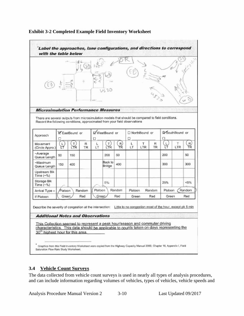
listed in the TVT are for a single point, not the entire segment). • State Highway Vehicle Classification Data

State Highway vehicle classification information is available through the TSM Unit’s Internet Traffic Volumes and Vehicle Classification webpage. Exhibit 3-3 shows an example excerpt of the State Highway Vehicle Classification Report. This report is also the source of information for highway segments AADT. With this information, the daily and hourly volumes can be obtained along with truck classifications which will substantially reduce the need for 48-hour road tube counts. Vehicle classes 4 through 13 are considered trucks for most applications, including Pavement Design and HCM analysis. However, class 3 vehicles may be considered light trucks in some software. Note that volumes listed in the State Highway Vehicle Classification report are for segments, as shown in Exhibit 3-3. A beginning mile point is shown for the starting point of each segment. Volumes listed in the Transportation Volume Tables are for individual points, as shown in Exhibit 3-4. The mile point shown is where the traffic count was taken.

Exhibit 3-3 Excerpt from State Highway Vehicle Classification Report

https://highway.odot.state.or.us/cf/highwayreports/traffic_parms.cfm


Exhibit 3-4 Excerpt from Transportation Volume Tables

• Automatic Traffic Recorders/Automatic Vehicle Classifiers (ATR/AVC) Sites

ATR and AVC sites record bidirectional volumes on an ongoing basis and can be used as substitutes for classification and regular road tube counts. ATR sites only include bidirectional volumes, but to understand vehicle classifications, every ATR site is also counted with a 24-hour classification count every three years which is available from the TSM Unit. AVCs continually classify data so classification data will be available throughout a given year at these locations. AVCs are gradually replacing ATRs so eventually all recorder sites will have classification abilities. ATR/AVC “Critical Hour” listings are also available which breakdown a year’s worth of data down to the hour level so a 30 HV can be easily obtained at that location. • Ramp Volume Diagrams While 16-hour counts at an interchange ramp terminal are preferable, the ramp volume diagrams in the Transportation Volume Tables and on the TSM Unit webpage can be used to substitute if a count is not available and intersection turn movements or intersection operations are not desired. Many of the interchange ramp volumes have 48-hour tube counts that were used to create these volumes, so an analyst should check for their availability. These counts are taken on a 3-year schedule. Free-flow ramp volumes (i.e. between two Interstate highways) can be obtained from the diagrams if a 48-hour tube count is not available or practical. The TVT ramp volumes are balanced and may not represent the actual count volumes. Contact the TSM Unit directly if the actual count is needed.

Other Jurisdiction’s Counting Programs In addition, some counties and larger cities may have traffic counting programs in place. The TSM Unit webpage also has links to many of these jurisdiction’s Internet traffic data pages on the Traffic Counting Program webpage. These counts are typically daily volumes and can be used to supplement the local system and can reduce the need for 48-hour road tube counts. Sometimes intersection counts are available, but differing classification breakdowns and durations from ODOT standards can make these difficult to use except for a source for local peak period counts.

https://www.oregon.gov/ODOT/Data/Pages/Traffic-Counting.aspx


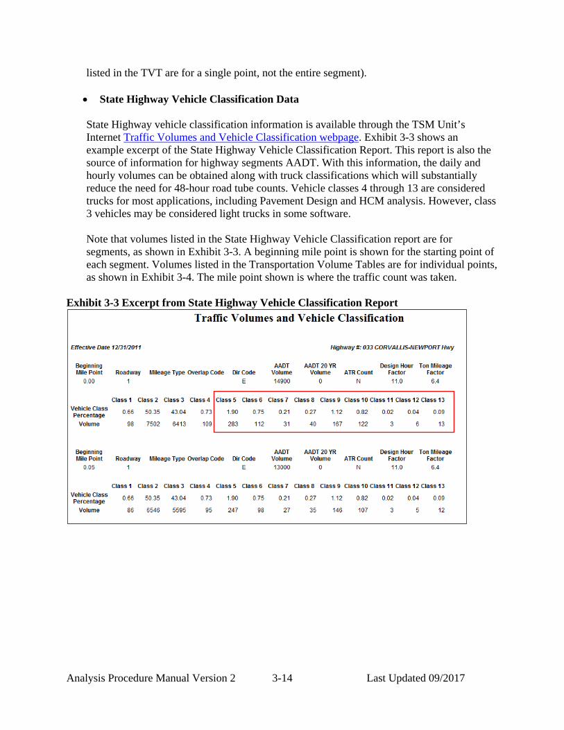
Traffic Signal Controller Counts The new Model-2070 and earlier Model-170 traffic signal controllers have the ability to store loop or video detection information that can be downloaded at a later date. This data is attractive to the end user as there are a large number of usable installations available. Controller count data is primarily used by Region signal timers, when preparing field refinements to signal timing plans. For traffic analysis, controller counts are useful in determining trends between weekday and weekend traffic, or in establishing relationships for side streets (i.e. seasonal adjustments). It is imperative to have a copy of the loop detector diagram for the specific intersection, when deciphering both Model-2070 and Model-170 controller count data. The Model-2070 controller stores the data in up to 32 columns or bins, depending on the complexity of the intersection, with two loops per detector phase (standard). However, field modifications may differ from the “as-built” plans, which is why a current detector diagram is necessary. The most recent detector diagrams can be obtained from the various Region Tech Centers. Special Vehicle Counts (short duration) Frequently on projects, there is a need to collect additional peak hour data for driveways, for a check count, or other overlooked spot. Sometimes these counts are done for specific purposes such as capturing headways, weaving movements, or saturation flow rates for simulation calibration. These counts typically are collected by the project analyst rather than region or consultant counting staff. Counts longer than an hour or in many locations should be done by region staff, TSM staff or traffic count contractors. These counts can be manually tabulated in case of a number of small adjacent driveway counts, or use of a video camera or electronic count board. Video cameras can be useful assuming that a good vantage point is available that will provide a clear view of all movements being counted. When using video cameras to collect count surveys, be sure to have an adequately charged battery and large enough media to collect the amount of data needed. Typically, when counts are not done by video, some sort of handheld electronic count device is used. One of these is the JAMAR board which has been used by ODOT in the past to collect counts. Limitations of the JAMAR boards prevent using these to do a full 13-class count. However, the boards can be used for volume-only or limited class counts. These counters are necessary for saturation flow data capture or other simulation/ operational data (see the Simulation Chapter). The JAMAR traffic count is in raw form which can be downloaded to a text file through the use of the serial cable and a communications program. Detailed instructions for this process are available on the Planning Section Technical Analysis and Tools webpage.

3.4.3 Vehicle Count Periods For most traffic studies, the 30th highest hour volumes (30 HV) should be used to represent future volumes. It is recommended a top 200- to 500-hour count listing (Critical Hour) of the ATR(s) is obtained from the Transportation Systems Monitoring Unit. The 30 HV at the ATR(s) will be included in the list so that it will be possible to determine when the 30 HV occurs during the day and in the week. Manual counts can then be timed for the period when the 30 HV will likely occur, minimizing seasonal adjustments. Exhibit 3-5 illustrates the general process for identifying when the 30 HV occurs. Refer to Chapter 5 for detailed guidance on each of these

https://www.oregon.gov/ODOT/Planning/Pages/Technical-Tools.aspx


steps. Exhibit 3-5 Determining When 30 HV Occurs

To get a typical traffic mix of the 30 HV for the analysis, the counts should be taken as close to the likely 30th highest hour as possible. This typically requires collecting counts on a weekday afternoon in most larger urban areas, but may include weekends for high recreation areas (the coast or Central Oregon), or areas experiencing lunch hour peaks or high reverse direction flows during the day. Where capturing school trips is important, counts need to be taken when school

ATR on sitewithin 10% of

AADT

ATR Characteristic Table

Seasonal Trend Table

Determine when 30HV occurs using top 200-500 listing

from ATR (s)

YES

NO

NO

YES

NO

Identify weekday or

weekend trend

YES

Is there a characteristic ATR (s)

YES


AADT




from ATR (s)

YES

NO

NO

YES

NO

Identify weekday or

weekend trend

YES


YES


AADT




from ATR (s)

YES

NO

NO

YES

NO

Identify weekday or

weekend trend

YES


YES


is in session. In some cases two sets of counts may be needed, during months when school is in session as well as during the summer. In fully developed portions of Metropolitan Planning Organization (MPO) areas, the 30th highest hour is generally assumed to be represented by the typical weekday evening commuter peak hour. Outside of fully developed MPO areas, a seasonal adjustment will be required to convert the counts to 30 HV. For access management, the peak hour is defined as the highest one-hour volume during a typical or average week in urban areas, and the 30th highest hourly volume on rural roadways. Seasonal adjustments should not be more than 30% because the traffic flow characteristics are most likely NOT represented by the count information. A seasonal adjustment greater than 30% indicates that the count was taken at the wrong time of year. Turn movement patterns may be so different they cannot be adequately represented by a seasonal adjustment. Count timing is critical especially if the project/plan SOW will not be complete until after October. Please refer to Existing Volume Development (Chapter 5) or contact the Transportation Planning Analysis Unit (TPAU) for advice. Counting Considerations to Minimize Seasonal Adjustments

• Coastal or summer recreational areas should be counted during the traditional summer period (Memorial Day to Labor Day). Outside of coastal/recreational areas, most areas can be counted from March to October. Larger MPO areas or commuter-based corridors can be counted most months, but should generally avoid December to February as these are the lowest traveled months, have a number of holidays, and have the most weather-related problems. Winter recreation areas (i.e. Mt. Hood area) should be counted in the December to February timeframe to capture the peak periods. Recreational areas (or routes that travel to or between recreational areas) may require counting on the weekends.

• If alternate periods/volume thresholds other than the typical summer/ or 30 HV like what would be used to create an alternate mobility standard, then counts need to be taken in those alternate periods so resulting seasonal factors do not exceed 30%. This might mean for certain efforts, multiple sets of count data may be required. For example, a summer recreational area that uses a non-summer standard, counts should be obtained in the non-summer (Oct-Apr) period. For areas that use an annual average, counts should be obtained in Sep-Oct and/or Apr-May periods. Winter or winter-summer recreational areas will be a variation/combination of the methods.

• Road tube count placement is limited to the April to October period because of studded tire damage potential.

• In general, days potentially influenced by state or federal holidays or other significant events (such as local festivals, sporting events, hunting season, etc.) that may alter normal traffic patterns should be avoided.

• Counts that may be influenced by nearby construction projects may be affected and such counts should be thoroughly investigated and may require adjustments.

• It is also common to avoid Monday and Friday counts when weekday data is desired, as the trip characteristics on these days generally differ from the remainder of the week.

• Consideration should be given to the presence of generators such as schools/colleges/universities because of the enrollment and events (such as spring break) can vary greatly through the year. Consideration should also be given to major


employers or attractions such as regional shopping centers that experience significant peaks in generated trips that may or may not occur during the other peaks because of shift changes or event scheduling. Note: The City of Corvallis requires that counts occur when OSU is in session because of the large percentage of the population related to school being in session.

• In agricultural areas, truck traffic may be highly seasonal and have a substantial impact on the system. Counts may have to be timed carefully to balance the overall peak months with the harvest periods.

• In the Portland Metro area, while infrequent, there may be times when additional data must be collected to capture the 2nd hour, needed to evaluate the adopted 2-hour OHP mobility target. This is generally only necessary when the mobility target for the second hour of the peak period is lower than the mobility target for the first hour of the peak period and the analysis shows the first hour does not meet its target, but satisfies the target for the second hour.

Counting Considerations for Congested Conditions Counting under congested conditions (i.e. Portland Metro area) requires some additional considerations as there may be places that the actual demand is queued up and unable to flow smoothly through the system. Volumes are being reflected on the ground while demand is being reflected in the form of unserved queues (cannot pass through in a single signal cycle over a 15-minute period at least) . In this case, a typical count would only measure the discharge flow through the intersection versus what would like to use the intersection. This could lead to an underestimation of demand especially under a build alternative condition. Both volume and demand should be quantified in the analysis in order to help inform the analyst on volume development steps and following analyses. If there is a suspicion that counts may not reflect true demand... Step 1: Check existing tube counts or automatic traffic recorders for any peak hour “M” effect

where the shoulder hours on each side of the peak hour/period are higher than the peak hour/period or the shoulder hours share the same capacity as the peak hour. If this is the case, demand has likely exceeded capacity.

Step 2: Check existing manual turning movement counts to see if the 15-minute shoulder intervals of the estimated peak hour/period are higher than the peak hour/intervals.

Step 3: If easily available, check private sector vehicle probe data such as TomTom or Inrix data to see if the corridor experiences speeds lower than the posted speed for more than one hour.

Step 4: Do a field visit or have video taken to verify whether vehicles can be served before ordering counts.

Step 5: Consider collecting counts upstream from the desired count location where the roadway is not oversaturated if congestion is observed in the field, video, and/or by counts. When counting upstream, consider counting side streets between the unsaturated count location and the desire count location that may have traffic leave or enter the roadway.

Other considerations:


• If traffic is heavily favoring a single lane more than others, lane by lane utilization counts or field observations are needed. For example, this can easily occur in one lane of a dual left turn lane because of an immediate lane drop or heavy turn movement downstream. Lane utilization counts should also be considered where a through lane is reduced downstream from a traffic signal.

• Locations need to be noted where queue spillback occurs from turn lanes blocking through lanes or vice versa. This may require additional counts upstream or field observations.

3.4.4 Vehicle Count Locations Vehicle count locations should be identified in the project work plan/SOW, and should be determined based on the needs of the subject plan or project. For example, planning efforts that are expected to generate potential highway projects within three years will require more detailed counts than a standalone or long-range plans, such as TSPs. For planning projects it is important to correspond with the local jurisdiction and TPAU/Region Traffic to make sure that count needs cover the system to be analyzed at the appropriate level of detail and address issues. The grant/project manager should meet with TPAU/Region Traffic staff to discuss traffic count requirements after the objective section of the SOW (or project prospectus) is completed as this section provides the context for the plan/project. For Transportation Growth Management (TGM) grants, it is usually more efficient to arrange a meeting with the appropriate TPAU/region staff to go over multiple studies at once. For construction projects, the project team or at least the region traffic engineer/manager, the environmental lead, and/or project leader should be consulted. While differences of opinion may exist on the number and type of counts versus the available budget, remember that the ultimate goal will be to have enough data to analyze and answer the questions, address the needs, evaluate alternatives, and cover the level of detail in the plan/project as described by the project objectives and the local jurisdiction(s). Staff will need to come to an agreement whether the data collection budget and/or the number/type of counts need to change. The following plan/project-specific count location guidelines do not cover every possibility or combination of elements, but are intended to help generate a reasonable starting point for discussion. The location guidelines are generally laid out in an increasing level of detail. County Transportation System Plan (TSP) The arterial and major collector system needs to be documented (counted). It is generally unnecessary to count lower functional class roads as these usually carry very little traffic, and possibly are unpaved unless the county government wants a specific roadway included because of operational issues. Analysis at the County level is more system-based with a higher emphasis on ADT rather than peak hour and many of the analysis tools require ADT as an input.

• Need to have at least ADT-level count coverage of the arterial and major collectors. Acceptable previously taken counts may exist at the state or local level.

• Major arterial intersections with other arterial and major collector intersections should be


counted where operational issues exist. State highway segments (between major intersections) should use the TSM Unit’s vehicle classification data to capture volumes and truck classifications.

• The TSM Unit’s ramp volume diagrams (where available) should be used to capture any free-flow ramp connections.

• County arterials and major collectors should have at least a 48-hour classification tube count performed so truck traffic can be captured and ADT can be calculated.

• Peak period counts should be obtained at signalized intersections, unsignalized highway to highway junctions, and county arterial – highway intersections. If this is a TSP Update, refer to the old TSP to help identify the critical intersections that should be counted.

City Transportation System Plan (TSP) The arterial and collector system needs to be documented (counted). It is generally unnecessary to count lower functional classes unless the roadway is area-significant, provides an alternate path for trips to bypass congested areas (as in a parallel local street), or the local government has previously identified operational issues. Analysis at the City level is more centered on the peak periods and individual facilities/intersections which require more detail.

• Need to have at least ADT-level count coverage of the arterial and collectors. Acceptable previously taken counts may exist at the state or local level.

• Major cities (> 50,000 pop,) generally need to have at least the arterial system counted. • Medium cities (10,000 – 49,999 pop.) generally need to have the arterial and

representative/significant collectors counted. • Small cities (<10,000 pop.) generally need to have the arterial and significant collectors

counted. • Major arterial intersections with other arterial and significant collector intersections

should be counted. Peak period counts should be obtained at minor arterial/collector signalized intersections, unsignalized highway to highway junctions, city arterial – highway intersections, and major private development accesses (i.e. regional shopping mall). If this is a TSP Update, refer to the old TSP to help identify the critical intersections that may need to be re-evaluated.

• Significant collectors extend across the city for a considerable distance, are a direct route, or extend outside the city.

• If multiple signals exist, it may not be necessary to have a count at every one, but a reasonable representation of the system needs to be counted.

• Bracketing peak period counts with 16-hour counts is an acceptable practice. Each major roadway should have truck traffic captured on it in at least one location.

• Sixteen-hour counts should be obtained at interchange ramp terminals and signalized major arterial intersections. If tube classification counts are available to provide ADT and truck volumes on each leg, then shorter duration counts can be used. The TSM Unit’s ramp volume diagrams (where available) should be used to capture any free-flow ramp connections.

• State highway segments (between major intersections) should use the TSM Unit’s vehicle classification data to capture volumes and truck classifications.

• City arterials and collectors should have at least a 48-hour tube count performed so ADT can be calculated. Larger cities may already have this count data.


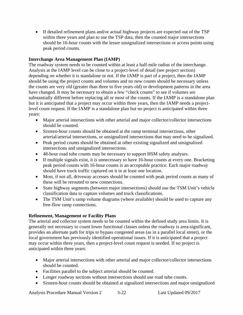
• If detailed refinement plans and/or actual highway projects are expected out of the TSP within three years and plan to use the TSP data, then the counted major intersections should be 16-hour counts with the lesser unsignalized intersections or access points using peak period counts.

Interchange Area Management Plan (IAMP) The roadway system needs to be counted within at least a half-mile radius of the interchange. Analysis at the IAMP level can be close to a project-level of detail (see project section) depending on whether it is standalone or not. If the IAMP is part of a project, then the IAMP should be using the project counts and volumes and no new counts should be necessary unless the counts are very old (greater than three to five years old) or development patterns in the area have changed. It may be necessary to obtain a few “check counts” to see if volumes are substantially different before replacing all or most of the counts. If the IAMP is a standalone plan but it is anticipated that a project may occur within three years, then the IAMP needs a project-level count request. If the IAMP is a standalone plan but no project is anticipated within three years:

• Major arterial intersections with other arterial and major collector/collector intersections should be counted.

• Sixteen-hour counts should be obtained at the ramp terminal intersections, other arterial/arterial intersections, or unsignalized intersections that may need to be signalized.

• Peak period counts should be obtained at other existing signalized and unsignalized intersections and unsignalized intersections.

• 48-hour road tube counts may be necessary to support HSM safety analyses. • If multiple signals exist, it is unnecessary to have 16-hour counts at every one. Bracketing

peak period counts with 16-hour counts is an acceptable practice. Each major roadway should have truck traffic captured on it in at least one location.

• Most, if not all, driveway accesses should be counted with peak period counts as many of these will be rerouted to new connections.

• State highway segments (between major intersections) should use the TSM Unit’s vehicle classification data to capture volumes and truck classifications.

• The TSM Unit’s ramp volume diagrams (where available) should be used to capture any free-flow ramp connections.

Refinement, Management or Facility Plans The arterial and collector system needs to be counted within the defined study area limits. It is generally not necessary to count lower functional classes unless the roadway is area-significant, provides an alternate path for trips to bypass congested areas (as in a parallel local street), or the local government has previously identified operational issues. If it is anticipated that a project may occur within three years, then a project-level count request is needed. If no project is anticipated within three years:

• Major arterial intersections with other arterial and major collector/collector intersections should be counted.

• Facilities parallel to the subject arterial should be counted. • Longer roadway sections without intersections should use road tube counts. • Sixteen-hour counts should be obtained at signalized intersections and major unsignalized


intersections (i.e., ramp terminals, four-way stops) to capture truck traffic or where larger scale improvements may be needed.

• Bracketing peak period counts with 16-hour counts is an acceptable practice. Each major roadway should have truck traffic captured on it in at least one location.

• Unsignalized intersections or major accesses should be counted with peak period counts. • 48-hour road tube counts may be necessary to support HSM safety analyses. • If an Interstate Highway or statewide expressway exists in the study area, the mainline

shall be counted by direction between interchanges in addition to any interchange ramp terminals. Road tube counts may be necessary to capture movements on ramps or connections.

Local Street Network (LSN) or Downtown Plan These kinds of plans are generally trying to identify new roadway or multimodal connections to control congestion on the state highway or make limited improvements in the downtown area. The arterial and collector system need to be counted. It is generally not necessary to count lower functional classes unless the roadway is the only access to a neighborhood, provides an alternate path for trips to bypass congested areas (as in a parallel local street), or the local government has previously identified operational issues. Larger numbers of peak period counts may be necessary with a few 16-hour counts at major intersections.

• Major arterial intersections with other arterial and collector intersections should be counted.

• Sixteen-hour counts should be obtained at signalized intersections and major unsignalized intersections (i.e., ramp terminals, four-way stops) to capture truck traffic or where larger scale improvements may be needed.

• If multiple signals exist, it is unnecessary to have 16-hour counts at each one. Each major roadway should have truck traffic captured on it in at least one location.

• Unsignalized intersections or major accesses should be counted with peak period counts. • 48-hour road tube counts may be necessary to support HSM safety analyses. • Bracketing peak period counts with 16-hour counts is an acceptable practice. Each major

roadway should have truck traffic captured on it in at least one location. • State highway segments (between major intersections) should use the TSM Unit’s vehicle

classification data to capture volumes and truck classifications. • The TSM Unit’s ramp volume diagrams should be used to capture any free-flow ramp

connections. Pedestrian or Trail Plans Generally, counts are only needed if the state highway system will be affected by removing or narrowing through travel lanes or if new crossings are to be added. Count requirements in the lane reduction areas should follow the LSN/Downtown Plan recommendations above. Plans with proposed mid-block trail crossings of state highways or local arterials should have a 48-hour classification road tube count performed at the crossing location. For plans with existing pedestrian crossings (formally defined or not) where the number of crossing pedestrians is desired, the crossing count should be replaced with a 16-hour video classification count with bike and pedestrians requested.


Pedestrian and/or bicycle counts are more adversely affected by weather conditions than vehicle counts, and are recommended to be taken when pedestrians and/or bikes are anticipated, such as not in the winter in many cases, or during school-in-session periods if near a school/college/university. Traffic Impact Studies (TIS) For TISs, the analysis area and study intersections are typically selected from estimates of anticipated impacts from added traffic based on site trip generation and distribution, and existing intersection operations. Count requests need to be developed with the guidance of the Region Access Management Engineer or appropriate region staff and the Development Review Guidelines.

• Sixteen-hour counts should be obtained at major unsignalized intersections (i.e., ramp terminals, four-way stops) to capture truck traffic; obtain the basis for signal warrants, or where larger scale improvements may be needed.

• Signalized intersections may use a 16-hour count or a peak period count depending on the particular study area.

• If multiple signals exist, it may not be necessary to have 16-hour counts at each one. Bracketing peak period counts with 16-hour counts is an acceptable practice. Each major roadway should have truck traffic captured on it in at least one location.

• Unsignalized intersections and accesses should be counted with peak period counts. • 48-hour road tube counts may be necessary to support HSM safety analyses. • The Interstate/expressway/highway mainline shall be counted by direction in addition to

any interchange ramp terminals. Road tube counts may be necessary to capture movements on ramps or connections.

Construction Projects For most other project types (modernization, safety, operations, etc) the analysis area and study intersections are selected by considering the problem that is being addressed by the project and the information that is required to fully assess the problem and propose appropriate solutions. Project analysis is needed to support roadway and intersection control improvements, pavement and bridge design, air quality, and noise mitigation. Larger projects, especially those with required environmental studies (such as noise and air quality) may require multiple full 16-hour classification counts.

• Sixteen-hour classification counts should be obtained at signalized intersections and major unsignalized intersections (i.e., ramp terminals, four-way stops) to capture truck traffic or where larger scale improvements may be needed.

• Truck classification data must be captured on each roadway segment in the study area. • Minor unsignalized intersections and accesses should be counted with peak period

counts. • 48-hour road tube counts may be necessary to support HSM safety analyses. • Significant driveway accesses should be counted as many of these will be rerouted to new

connections. • If an Interstate Highway or grade-separated highway exists in the study area, the mainline


must be counted by direction between interchanges in addition to any interchange ramp terminals. Road tube counts may be necessary to capture movements on ramps or connections.

3.4.5 ODOT Internal Count Request Process When ordering counts, the request must contain the name of the contact person (requestor), the person to whom the data will be sent, the locations, time periods, dates, types of counts and collection methods must be clearly communicated to those conducting the counts. Count requests should group different count types (classification, peak period, road tube) separately for clarity. The count request should also list any special requests, count intervals, count time windows (start and finish dates), and a charge number (Expenditure Account (EA) for internal counts). A couple examples of a special request would be counting only on a specific day or counting certain intersections or elements of intersections at the same time. Because of staffing restrictions, classification counts for 2012 and beyond will not have pedestrian and bikes counted by default. Pedestrians and bike counts will need to be specifically requested. A map showing the count locations, durations and other special requirements should also be provided to help eliminate misunderstandings since often times the text is separated from the map. Please keep in mind that the field counting staff usually only has the map in hand so all pertinent information (count locations, durations, types, intervals, and special requests) needs to be on the map. A Sample Count Request including map have been included in Appendix 3B. When ordering intersection counts, be sure to specify the duration and type for each location. Fifteen-minute intervals must be specified for at least the standard morning, noon and evening peak periods in 16-hour counts. Peak period counts should be done in 15-minute intervals. It is not required, but very helpful if 48-hour road tube counts are counted in 15-minute intervals as well. Specify the latest acceptable date by which the count is needed for analysis. Keep in mind, based on scheduling and staff limitations, that it can take at least five weeks from the date of the request date to get the count scheduled (not including weather restrictions) and then another three to four weeks to have the count processed, recorded and distributed. Therefore, counts need to be requested about nine weeks ahead (or more if weather is a factor) of when they will be needed for the analysis work. All count requests should have copies sent to both the Region Traffic Manager and to the TSM unit to alert them that they are requested and need to be scheduled. Either TSM or the region staff will have the counts performed (in-house or with contractors) and should assure that the data is processed into an ODOT format before being released to the requestor. The TSM Unit needs know what counts are available so staff resources can be allocated. The TSM Unit coordinates the counting schedules of all Region traffic counting staff. Coordinating with the TSM Unit in the loop allows for these counts to be added to ensure the count databases are properly maintained, which can avoid unnecessary duplication and limit counting needs by others and minimize delays. ADT –capable counts performed by third parties or consultants are also encouraged to be submitted to the TSM Unit to be added to the database.



3.4.6 Using the Traffic Count Management (TCM) Program (ODOT Employees Only) TCM is a program maintained by the TSM Unit and available for installation on ODOT staff computers. It contains recent counts (2008 forward) conducted throughout the state of Oregon. Counts performed by the TSM Unit and counts provided to the TSM Unit are entered into the program. It is important to contact the TSM Unit if you are unable to find counts in your study area or to determine if there are existing counts that have not been processed. There are many different count types and each requires TCM to generate a different report. TCM must be installed on a computer and an individual user name and password is required. Contact the TSM Unit for access. The Traffic Count Management (TCM) Program Count Report Guide, included in Appendix 3C, provides step-by-step instructions on how to obtain traffic count information from TCM in the correct format for the most common types of counts used by the analyst. This includes intersection counts, ATR/AVC sites, TruckSum, and tube (machine) counts.

3.4.7 Count Validation Once counts are completed and processed and are available to the analyst , the counts should be checked to make sure that everything is furnished as requested. This includes count days, time periods, 15-minute intervals, movements, and classification requirements. Missing data, intersection approaches, etc should be reported back to the TSM Unit and the appropriate region for recounting (if possible) or reprocessing (in case of a video count) as soon as possible. Do not wait until all of the counts are completed to perform these checks. Check the counts for any “red flags.” Do the values look okay? Counts have had approaches mis-labeled, or wrong orientations (i.e.flipped east to west but also can be west to north) . As counts are being assembled for volume development, additional issues may arise between adjacent counts. Compare these counts with previous counts with adding in factored historical/seasonal growth; they should be similar if nothing has changed in the field between the counts. If adjacent or a whole section of counts appear to be very low or high, then verify that no incidents (road closures on the subject or adjacent roadways, crashes, bad weather, or scheduled events nearby) occurred while the count was in progress. If the count is 18 months or older then crash data records can be checked. Recent counts may require more investigation (contact TSM Unit, Region traffic units, local maintenance districts, or traffic operation centers).

3.5 Travel Time, Speed and Other Data Collection

3.5.1 Travel Time Travel time surveys measure the duration of time taken for a vehicle to travel from one point to another along a designated route, and are often used to quantify congestion over a corridor. The data collected from travel time surveys works well with statistical analysis, and the results are

https://www.oregon.gov/ODOT/Planning/Documents/APMv2_App3C.pdf


often more easily understood by the public than other methods used for measuring congestion. Data Collection One common method used for this data collection uses a “floating car.” The elapsed time is measured from a car driven along the designated route maintaining an average travel speed relative to other cars on the road. Other methods include vehicle or license plate matching and the use of various intelligent transportation system technologies. Travel time data is collected at the beginning and end of a designated route, and can be collected between predetermined points along the route as well, depending on the level of information desired. Travel time can also be calculated from Inrix speed data using the average speed and segment length (see section on Speed below). When collecting travel time data, all measurements should be taken under good weather conditions and during a time representative of the period of interest for the study. Except when collecting the data for simulation calibration, it is good to distribute the travel time runs over several days and over multiple weeks that are representative. To have an accurate representation of the field conditions for simulation calibration, travel times need to be taken at the same time as the operational field data collection. It is recommended that a minimum of 10 travel time runs be collected in each direction for each hour to be simulated (and each lane where lane imbalances occur) for both freeways and arterials. The 10 travel time runs should be collected during the same time as other data collection if possible but can be collected over multiple days if necessary. The travel time runs can also be a combination of the floating car and Bluetooth data methods. For VISSIM simulations, refer to Section 3.5 in the VISSIM Protocol. Floating Car Data Collection with GPS Floating car travel time runs are conducted using a handheld GPS device that records vehicle location, speed, and direction of travel every 1 to 5 seconds. This method allows the actual roadway conditions to be analyzed as the data returned from the probe vehicles will reflect the periods of congestion and free-flow speeds experienced by other motorists. The floating car technique requires the driver to mimic or match the speed of the traffic stream for a given roadway. However, it may be difficult for test drivers to mirror the actions of the traffic stream as drivers often revert to their own driving habits instead of staying with the majority of traffic. When designing a floating car study, the goal is to have a large enough sample which is optimally spaced for the purpose of capturing variability within the traffic stream. Some things to consider:

1. Route selection a. Try to include as many key intersections, segments as necessary

2. The number of floating car “probes” and the area (route) covered per run a. In general, increasing the number of probes sampled during the run and/or

reducing the area size will increase the resolution of the samples. 3. Lane position of probe car

a. Results are provided in fine enough detail to determine speeds based on lanes occupied. It may be difficult for the driver to determine which lane most closely represents the average vehicle speed.


4. Weather, Tree cover and %trucks along route. a. High instances of either will lead to signal disruption and loss of data points.

5. Start the routes at least 15 minutes ahead of recording period a. Establishing the route prior to the recording time minimizes driver route errors

6. Driver Notes are helpful (see Exhibit 3-5 Determining When 30 HV Occurs). a. Record queue position at intersections b. Lane position

Exhibit 3-6 Example of Notes

Upon completion of the of the floating car runs, the data is downloaded to an ArcGIS shapefile format for cleaning and analysis (see Exhibit 3-7). It is typical that some data cleaning will be required such as removing outliers and converting the speed to MPH. This is easily done in ArcGIS. Exhibit 3-7 Data format

Example 3-1 Floating Car Data Collection with GPS For a project in Albany, travel time data is needed for calibration of a simulation model for the Existing Year. See Chapter 15 for calibration procedures. Floating car data was collected on March 31st 2010 in the peak hour between 4:45 PM and 5:45 PM. Three vehicles were equipped with GPS units and each assigned a separate travel route. In order to represent the most likely driving conditions drivers were asked to travel according to their best judgment of the traffic stream's speed and collect as many full routes as possible during the data collection period.


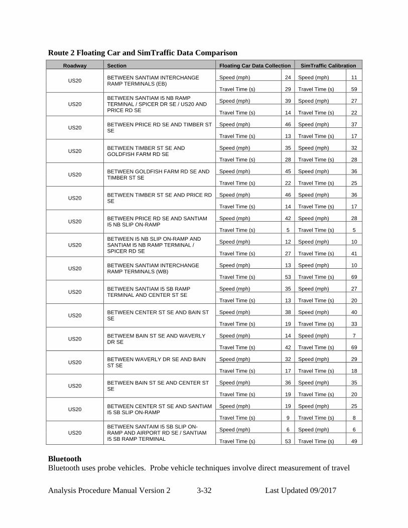
Average speeds along the routes were recorded in the GPS tracklog where time/location points set to record at 1 second intervals. A greater interval period could be used in other applications such as for a rural corridor. At each 1 second interval, the GPS recorded the coordinate location, the date and time the data point was recorded and the instantaneous speed of the vehicle. Instantaneous speed and travel times along each route were averaged over the total number of completed runs and summarized based on link segments from the SYNCHRO network. The figures below display the floating car data collection route and output results. The table below summarizes the results of the data collection.


Floating Car Data Collection, Route 2


Floating Car Data Output Results


Route 2 Floating Car and SimTraffic Data Comparison

Bluetooth Bluetooth uses probe vehicles. Probe vehicle techniques involve direct measurement of travel

Roadway Section Floating Car Data Collection SimTraffic Calibration

US20 BETWEEN SANTIAM INTERCHANGE RAMP TERMINALS (EB)

Speed (mph) 24 Speed (mph) 11

Travel Time (s) 29 Travel Time (s) 59

US20 BETWEEN SANTIAM I5 NB RAMP TERMINAL / SPICER DR SE / US20 AND PRICE RD SE



US20 BETWEEN PRICE RD SE AND TIMBER ST SE



US20 BETWEEN TIMBER ST SE AND GOLDFISH FARM RD SE



US20 BETWEEN GOLDFISH FARM RD SE AND TIMBER ST SE



US20 BETWEEN TIMBER ST SE AND PRICE RD SE



US20 BETWEEN PRICE RD SE AND SANTIAM I5 NB SLIP ON-RAMP



US20 BETWEEN I5 NB SLIP ON-RAMP AND SANTIAM I5 NB RAMP TERMINAL / SPICER RD SE



US20 BETWEEN SANTIAM INTERCHANGE RAMP TERMINALS (WB)



US20 BETWEEN SANTIAM I5 SB RAMP TERMINAL AND CENTER ST SE



US20 BETWEEN CENTER ST SE AND BAIN ST SE



US20 BETWEEM BAIN ST SE AND WAVERLY DR SE



US20 BETWEEN WAVERLY DR SE AND BAIN ST SE



US20 BETWEEN BAIN ST SE AND CENTER ST SE



US20 BETWEEN CENTER ST SE AND SANTIAM I5 SB SLIP ON-RAMP



US20 BETWEEN SANTAIM I5 SB SLIP ON-RAMP AND AIRPORT RD SE / SANTIAM I5 SB RAMP TERMINAL




time (along a route or point to point) using data from a portion of the vehicle stream. Probe measure technology (cell phone triangulation or GPS location tracking) is based on collecting vehicle ID data and timestamps of vehicles passing a roadside reader device and checking against the last reader passed to determine the travel time between reader locations. Many computers, car radios, navigation devices, PDA’s, cell phones, headsets and other personal devices are Bluetooth enabled to allow wireless communication between devices. Both types of probe technologies provide direct travel time output. Bluetooth-based travel time measurement involves identifying and matching the MAC address of blue-tooth enabled devices. This can be used to measure arterial travel time, average running speed, and OD patterns of travelers (see sections below). There have been several recent studies evaluating the effectiveness of the bluetooth device matching method compared to ground truck data. The results indicate that blue tooth is capable of reproducing floating car data, while providing a significantly higher number of data points than the floating car method.

3.5.2 Speed Speed data is used in multiple areas of analysis. There are measured and calculated speeds. A measured speed is a direct “point” measurement obtained with the use of equipment such as road tubes, Radar, or Lidar. A calculated speed is derived from a combination of a time and distance information (i.e. travel time over a specific length segment). Measured Speed One of the easiest ways to obtain a measured speed is through the use of road tubes with vehicle classifying counter. This method can only be used for free-flow non-congested segments where tubes can be safely placed, outside the influence of any intersections causing platooning effects. Collection of tube count data is restrained by weather and installation issues and needs to be coordinated with count program staff. Another method to obtain a measured speed is through the use of hand-held speed devices such as Radar/Lidar. See the Speed Zone Investigations Manual for procedures for measuring speeds with these devices. Measured speeds can be used to calculate segment speeds and headways. A measured speed may also be needed to determine/verify a specific segment speed such as a turning speed around a “non-standard” radius or corner for the purpose of simulation. Speed data can also be obtained from fee-based private sources, such as Inrix. Inrix is a private-sector provider of travel time and speed data at the link level worldwide with over 400 different sources of input data (mobile, fleet, in-pavement, etc). Inrix speed is based on GPS observations from fleets of probe vehicles (mostly commercial) which capture speed along major roadway segments. Average speed is available for every hour of the year. The travel time is calculated from the average speed and segment length. ODOT has purchased an Inrix historical archive of real time data covering the state of Oregon.

https://www.oregon.gov/ODOT/Engineering/TRSDocs/Speed-Zone-Manual.pdf


The historical data is a comprehensive database of speed statistics by day of the week. In rural or smaller urban areas, data coverage is generally limited to state highways (which have the most probe vehicles). Larger urban areas are more likely to include data on non-state facilities. ODOT has also purchased Inrix Analytics, a web-based tool which facilitates data extraction and reporting. The Analytics Tool is available at www.inrixtraffic.us. The Analytics Tools uses historical 1-minute or 5-minute bins of real-time data with TMC, speeds, travel times and quality scores. Quality scores indicate whether the data is based on real-time, average, or reference speeds (30, 20, or 10 respectively). Scores of “30” also have a confidence value (0-100) which indicates consistency with itself, the average, and overall trends. Public agencies within Oregon can freely use the data for planning and analysis. ODOT can authorize contractors to do the same on ODOT’s behalf. Some limitations are that Inrix data cannot be merged or averaged with competitor’s data (i.e. Tom-Tom) and that Inrix must be given credit when the data is used. Contact the ODOT ITS Unit for more information on data availability. Calculated Speed Calculated speeds are obtained from sources that furnish point or vehicle identification with a time stamp so data matching can yield a time between known points to determine an average speed. Data may be obtained from vehicle detection equipment, historic data or private sector sources. Common uses for calculated speeds are for calibration and validation of simulation models and creation of performance measures. Floating car and MAC address matched travel time data can be converted into “running speed”, segment or corridor travel speeds as long as distances are available.

3.5.3 Other Data Collection Origin-Destination (O-D) Surveys These surveys obtain route information that a vehicle takes between specific points. Project complexity can range from simple, such as a weave study, to medium focusing on select paths within a project/study area, to complex such as a city-wide network. The number of “interview” stations adds complexity to the process.

o Direct Interview - This process entails stopping a sample of vehicles to ask specific data collection such as point of beginning and ending, trip purpose, route choice, etc. Sometimes these are viewed as disruptive and invading privacy. These are very expensive (labor and traffic control) and require Oregon Transportation Commission (OTC) approval for state highways because of impacts to the traffic flows.

o License Plate Surveys – This process uses in-person or recorder images of vehicle identification (license plates) to obtain routing information without the stops associated with a direct interview process. This method can be expensive and labor intensive to match the data inputs. The more stations that are recorded, the more complex the process.

o Mail Survey – This process uses a sampling method to deliver/receive route information from driver input. This method requires a large distribution of requests to

http://www.inrixtraffic.us/

https://www.oregon.gov/ODOT/Maintenance/Pages/ITS-Operations.aspx


get a valid sampling of information. It can have accuracy (driver reporting), privacy and timeliness issues.

o MAC Address Reader (Bluetooth) - This process uses roadside detectors (portable or permanent) to record an identifying signature of an electronic device. Using multiple detectors, the device can be tracked to a specific route. To alleviate privacy issues, only a minimal amount of characters needed to uniquely specify a device is recorded. The electronic files of data can be matched using software programs, thus reducing labor costs.

Saturation Flow Rate Studies The saturation flow rate is a critical component in signalized intersection analysis. It is defined as the flow in vehicles per hour accommodated by a lane group assuming that the green phase is displayed 100 percent of the time. Saturation flow rate data is collected on an ongoing basis. Oregon saturation flow studies done to date show that the HCM 2010 value of 1750 passenger cars per hour of green per lane is appropriate for small urban areas. Except in larger urban areas, field conditions generally do not allow the HCM saturation flow study procedures in Chapter 31 of the 2010 HCM to be met. A roadway approach may not have long enough queues during the study or intersection spacing may be so tight that long enough queues without gaps are not possible. In these cases, a default ideal unadjusted saturation flow is determined as follows:

• Outside of the Portland, Salem and Eugene MPO urban areas the unadjusted saturation flow rate is 1750 passenger cars per hour of green per lane (pcphgl).

• Inside the Portland, Salem and Eugene MPO urban growth boundaries an unadjusted saturation flow rate of 1900 pcphgl may be used, unless one or more of the following conditions is present, in which case 1750 pcphgl shall be used. Conditions indicating use of lower base saturation flow rate inside urban growth boundaries:

o On-street parking o Greater than 5% trucks o Roadways intersect at severe skew angle (i.e., greater than 20 degrees off

perpendicular) o One or more driveway approach(es) with a combined volume in excess of 5 vph,

are present downstream of the intersection within the functional area (see Chapter 4) or upstream within the length of the standing queue

o Poor signal spacing or observed queue spillbacks between signals during the peak hour

o Less than 12-foot travel lanes

The ideal (unadjusted) saturation flow rate is converted to an actual flow rate by applying adjustment factors to account for the influence of lane widths, heavy vehicles, approach grades, on-street parking, frequent bus stoppages (3-4 or more per hour per direction) in the intersection vicinity or roadway segment, area type, lane utilization, turning movements and bicycle and pedestrian conflicts. Theoretically, once adjusted, the result would be equivalent to the field measured value.


Field Measurements of Saturation Flow Rates When an analyst desires a verification of the saturation flow (conditions are outside the default conditions above or a need for simulation), an investigation should be performed. The field measurement of the saturation flow rate shall be in accordance with methodology described in Chapter 31 of the 2010 Highway Capacity Manual (HCM) and submitted on the HCM Field Saturation Flow Rate Field Study Worksheet(s). The measurement is performed by recording the following data for each signal cycle and each desired lane. In order for a cycle to be used, it needs to have a minimum of 8 vehicles in the stopped queue at the start of green. First record the number of vehicles in the stopped queue when the signal turns green. Then record the elapsed time elapsed between when the front axle of the fourth vehicle in queue crosses the stop line and when the front axle of the last vehicle in queue crosses the stop line. Finally record the end of green. These values are used to calculate the average saturation flow headway per vehicle. Signal cycles with events such as downstream queues blocking the flow of traffic or presence of emergency vehicles should be discarded. A minimum of 15 signal cycles with a minimum of 8 vehicles in the stopped queue is needed to obtain a statistically significant value.

Saturation Headway = (Time of last stopped vehicle - Time of 4th vehicle) (Vehicle position of last vehicle - 4)

Saturation Flow = 3600 s/h saturation headway

In order to facilitate this process, a Saturation Flow Rate Data Collection Form and a Saturation Flow Rate Calculator tool have been developed. The data collection form is arranged as one row per cycle. For each cycle, the analyst records the time of the 4th vehicle, time of last stopped vehicle, number of stopped vehicles and time at end of green. Once collected, the data from the form are directly entered into the calculator office form tab. If more than 25 cycles of data have been collected, additional cycles can be added to the calculator by pressing the “Add 25 More Cycles” button. Once the analyst has input the field data, click the “Calculate Sat Flow” button. The calculator automatically checks to ensure there are at least 15 cycles with 8 or more vehicles in queue. Cycles with less than 8 vehicles in queue are ignored. For more specifics on the tool see the Instructions tab. Field measured saturation flow rates are preferred over estimation and do not require further modification. Using default values and adjustment factors will not produce more accurate results. If possible, saturation flow rates should be collected at no less than one major intersection on each main study area roadway. When using these values in analysis be sure to set all of the adjustment factors to 1.0. Once the field saturated flow rate is obtained, the ideal (unadjusted) saturation flow rate should be back-calculated by applying adjustment factors to account for the influence of lane widths,

https://www.oregon.gov/ODOT/Planning/Documents/APMv2_App3D.pdf

https://www.oregon.gov/ODOT/Planning/Documents/SatFlowCalculator.xls

https://www.oregon.gov/ODOT/Planning/Documents/SatFlowCalculator.xls


heavy vehicles, approach grades, on-street parking, bus stops, area type, lane utilization, turning movements and bicycle and pedestrian conflicts. Heavy vehicles, parking maneuvers, turning movements, and bicycle and pedestrian conflicts must be collected during the same period as the field saturation flow study to be able to back- calculate an accurate value. TPAU has a limited database of saturation flow rates. To find out if specific saturation flow rates are available for a specific site/area, contact TPAU analysts. Copies of saturation flow rate studies should be sent to TPAU for inclusion in appropriate studies such as verification of default values. Coordinate data collection and verification with TPAU so any acceptable saturation flow studies can be included in the database.


Appendix 3A – Field Inventory Worksheet

Appendix 3B – Sample Count Request and Sample ODOT Counts

Appendix 3C – Traffic Count Management (TCM) Program Count Report Guide

Appendix 3D – Saturation Flow Rate Data Collection Form





https://www.oregon.gov/ODOT/Planning/Documents/APMv2_App3D.pdf

3 TRANSPORTATION SYSTEM INVENTORY - Oregon Procedure Manual Version 2 3-1 Last Updated 09/2017 3...

Documents

Transcript of 3 TRANSPORTATION SYSTEM INVENTORY - Oregon Procedure Manual Version 2 3-1 Last Updated 09/2017 3...