3 Rademacher Complexity and VC- Dimension

3 Rademacher Complexity and VC-

Dimension

The hypothesis sets typically used in machine learning are infinite. But the samplecomplexity bounds of the previous chapter are uninformative when dealing withinfinite hypothesis sets. One could ask whether efficient learning from a finite sampleis even possible when the hypothesis set H is infinite. Our analysis of the family ofaxis-aligned rectangles (Example 2.1) indicates that this is indeed possible at leastin some cases, since we proved that that infinite concept class was PAC-learnable.Our goal in this chapter will be to generalize that result and derive general learningguarantees for infinite hypothesis sets.

A general idea for doing so consists of reducing the infinite case to the analysisof finite sets of hypotheses and then proceed as in the previous chapter. Thereare different techniques for that reduction, each relying on a different notion ofcomplexity for the family of hypotheses. The first complexity notion we will useis that of Rademacher complexity . This will help us derive learning guaranteesusing relatively simple proofs based on McDiarmid’s inequality, while obtaininghigh-quality bounds, including data-dependent ones, which we will frequently makeuse of in future chapters. However, the computation of the empirical Rademachercomplexity is NP-hard for some hypothesis sets. Thus, we subsequently introducetwo other purely combinatorial notions, the growth function and the VC-dimension.We first relate the Rademacher complexity to the growth function and then boundthe growth function in terms of the VC-dimension. The VC-dimension is often easierto bound or estimate. We will review a series of examples showing how to computeor bound it, then relate the growth function and the VC-dimensions. This leads togeneralization bounds based on the VC-dimension. Finally, we present lower boundsbased on the VC-dimension both in the realizable and non-realizable cases, whichwill demonstrate the critical role of this notion in learning.

34 Rademacher Complexity and VC-Dimension

3.1 Rademacher complexity

We will continue to use H to denote a hypothesis set as in the previous chapters,and h an element of H. Many of the results of this section are general and hold foran arbitrary loss function L : Y × Y → R. To each h : X → Y, we can associate afunction g that maps (x, y) ∈ X ×Y to L(h(x), y) without explicitly describing thespecific loss L used. In what follows G will generally be interpreted as the family ofloss functions associated to H.

The Rademacher complexity captures the richness of a family of functions bymeasuring the degree to which a hypothesis set can fit random noise. The followingstates the formal definitions of the empirical and average Rademacher complexity.

Definition 3.1 Empirical Rademacher complexityLet G be a family of functions mapping from Z to [a, b] and S = (z1, . . . , zm) a fixedsample of size m with elements in Z. Then, the empirical Rademacher complexityof G with respect to the sample S is defined as:

RS(G) = Eσ

[supg∈G

1m

m∑i=1

σig(zi)

], (3.1)

where σ = (σ1, . . . , σm)�, with σis independent uniform random variables takingvalues in {−1, +1}.1 The random variables σi are called Rademacher variables.

Let gS denote the vector of values taken by function g over the sample S: gS =(g(z1), . . . , g(zm))�. Then, the empirical Rademacher complexity can be rewrittenas

RS(G) = Eσ

[supg∈G

σ · gS

m

].

The inner product σ · gS measures the correlation of gS with the vector of randomnoise σ. The supremum supg∈G

σ·gS

m is a measure of how well the function class G

correlates with σ over the sample S. Thus, the empirical Rademacher complexitymeasures on average how well the function class G correlates with random noiseon S. This describes the richness of the family G: richer or more complex familiesG can generate more vectors gS and thus better correlate with random noise, onaverage.

1. We assume implicitly that the supremum over the family G in this definition ismeasurable and in general will adopt the same assumption throughout this book for othersuprema over a class of functions. This assumption does not hold for arbitrary functionclasses but it is valid for the hypotheses sets typically considered in practice in machinelearning, and the instances discussed in this book.

3.1 Rademacher complexity 35

Definition 3.2 Rademacher complexityLet D denote the distribution according to which samples are drawn. For anyinteger m ≥ 1, the Rademacher complexity of G is the expectation of the empiricalRademacher complexity over all samples of size m drawn according to D:

Rm(G) = ES∼Dm

[RS(G)]. (3.2)

We are now ready to present our first generalization bounds based on Rademachercomplexity.

Theorem 3.1

Let G be a family of functions mapping from Z to [0, 1]. Then, for any δ > 0, withprobability at least 1 − δ, each of the following holds for all g ∈ G:

E[g(z)] ≤ 1m

m∑i=1

g(zi) + 2Rm(G) +

√log 1

δ

2m(3.3)

and E[g(z)] ≤ 1m

m∑i=1

g(zi) + 2RS(G) + 3

√log 2

δ

2m. (3.4)

Proof For any sample S = (z1, . . . , zm) and any g ∈ G, we denote by ES [g] theempirical average of g over S: ES [g] = 1

m

∑mi=1 g(zi). The proof consists of applying

McDiarmid’s inequality to function Φ defined for any sample S by

Φ(S) = supg∈G

E[g] − ES [g]. (3.5)

Let S and S′ be two samples differing by exactly one point, say zm in S and z′min S′. Then, since the difference of suprema does not exceed the supremum of thedifference, we have

Φ(S′) − Φ(S) ≤ supg∈G

ES [g] − ES′ [g] = supg∈G

g(zm) − g(z′m)m

≤ 1m

. (3.6)

Similarly, we can obtain Φ(S) − Φ(S′) ≤ 1/m, thus |Φ(S) − Φ(S′)| ≤ 1/m. Then,by McDiarmid’s inequality, for any δ > 0, with probability at least 1 − δ/2, thefollowing holds:

Φ(S) ≤ ES[Φ(S)] +

√log 2

δ

2m. (3.7)


We next bound the expectation of the right-hand side as follows:

ES[Φ(S)] = E

S

[supg∈H

E[g] − ES(g)]

= ES

[supg∈H

ES′

[ES′(g) − ES(g)

]](3.8)

≤ ES,S′

[supg∈H

ES′(g) − ES(g)]

(3.9)

= ES,S′

[supg∈H

1m

m∑i=1

(g(z′i) − g(zi))]

(3.10)

= Eσ,S,S′

[supg∈H

1m

m∑i=1

σi(g(z′i) − g(zi))]

(3.11)

≤ Eσ,S′

[supg∈H

1m

m∑i=1

σig(z′i)]

+ Eσ,S

[supg∈H

1m

m∑i=1

−σig(zi)]

(3.12)

= 2 Eσ,S

[supg∈H

1m

m∑i=1

σig(zi)]

= 2Rm(G). (3.13)

Equation 3.8 uses the fact that points in S′ are sampled in an i.i.d. fashion and thusE[g] = ES′ [ES′(g)], as in (2.3). Inequality 3.9 holds by Jensen’s inequality and theconvexity of the supremum function. In equation 3.11, we introduce Rademachervariables σis, that is uniformly distributed independent random variables takingvalues in {−1, +1} as in definition 3.2. This does not change the expectationappearing in (3.10): when σi = 1, the associated summand remains unchanged;when σi = −1, the associated summand flips signs, which is equivalent to swappingzi and z′i between S and S′. Since we are taking the expectation over all possible S

and S′, this swap does not affect the overall expectation. We are simply changing theorder of the summands within the expectation. (3.12) holds by the sub-additivity ofthe supremum function, that is the identity sup(U +V ) ≤ sup(U)+sup(V ). Finally,(3.13) stems from the definition of Rademacher complexity and the fact that thevariables σi and −σi are distributed in the same way.

The reduction to Rm(G) in equation 3.13 yields the bound in equation 3.3,using δ instead of δ/2. To derive a bound in terms of RS(G), we observe that,by definition 3.2, changing one point in S changes RS(G) by at most 1/m. Then,using again McDiarmid’s inequality, with probability 1 − δ/2 the following holds:

Rm(G) ≤ RS(G) +

√log 2

δ

2m. (3.14)

Finally, we use the union bound to combine inequalities 3.7 and 3.14, which yields

3.1 Rademacher complexity 37

with probability at least 1 − δ:

Φ(S) ≤ 2RS(G) + 3

√log 2

δ

2m, (3.15)

which matches (3.4).

The following result relates the empirical Rademacher complexities of a hypothe-sis set H and to the family of loss functions G associated to H in the case of binaryloss (zero-one loss).

Lemma 3.1

Let H be a family of functions taking values in {−1, +1} and let G be the family ofloss functions associated to H for the zero-one loss: G = {(x, y) �→ 1h(x) �=y : h ∈ H

}.

For any sample S = ((x1, y1), . . . , (xm, ym)) of elements in X × {−1, +1}, let SXdenote its projection over X : SX = (x1, . . . , xm). Then, the following relation holdsbetween the empirical Rademacher complexities of G and H:

RS(G) =12RSX (H). (3.16)

Proof For any sample S = ((x1, y1), . . . , (xm, ym)) of elements in X × {−1, +1},by definition, the empirical Rademacher complexity of G can be written as:

RS(G) = Eσ

[suph∈H

1m

m∑i=1

σi1h(xi) �=yi

]= E

σ

[suph∈H

1m

m∑i=1

σi1−yih(xi)

2

]=

12

Eσ

[suph∈H

1m

m∑i=1

−σiyih(xi)]

=12

Eσ

[suph∈H

1m

m∑i=1

σih(xi)]

=12RSX (H),

where we used the fact that 1h(xi) �=yi= (1− yih(xi))/2 and the fact that for a fixed

yi ∈ {−1, +1}, σi and −yiσi are distributed in the same way.

Note that the lemma implies, by taking expectations, that for any m ≥ 1, Rm(G) =12Rm(H). These connections between the empirical and average Rademacher com-plexities can be used to derive generalization bounds for binary classification interms of the Rademacher complexity of the hypothesis set H.

Theorem 3.2 Rademacher complexity bounds – binary classificationLet H be a family of functions taking values in {−1, +1} and let D be the distributionover the input space X . Then, for any δ > 0, with probability at least 1 − δ over


a sample S of size m drawn according to D, each of the following holds for anyh ∈ H:

R(h) ≤ R(h) + Rm(H) +

√log 1

δ

2m(3.17)

and R(h) ≤ R(h) + RS(H) + 3

√log 2

δ

2m. (3.18)

Proof The result follows immediately by theorem 3.1 and lemma 3.1.

The theorem provides two generalization bounds for binary classification based onthe Rademacher complexity. Note that the second bound, (3.18), is data-dependent:the empirical Rademacher complexity RS(H) is a function of the specific sampleS drawn. Thus, this bound could be particularly informative if we could computeRS(H). But, how can we compute the empirical Rademacher complexity? Usingagain the fact that σi and −σi are distributed in the same way, we can write

RS(H) = Eσ

[suph∈H

1m

m∑i=1

−σih(xi)]

= −Eσ

[inf

h∈H

1m

m∑i=1

σih(xi)].

Now, for a fixed value of σ, computing infh∈H1m

∑mi=1 σih(xi) is equivalent to

an empirical risk minimization problem, which is known to be computationallyhard for some hypothesis sets. Thus, in some cases, computing RS(H) couldbe computationally hard. In the next sections, we will relate the Rademachercomplexity to combinatorial measures that are easier to compute.

3.2 Growth function

Here we will show how the Rademacher complexity can be bounded in terms of thegrowth function.

Definition 3.3 Growth functionThe growth function ΠH : N → N for a hypothesis set H is defined by:

∀m ∈ N, ΠH(m) = max{x1,...,xm}⊆X

∣∣∣{(h(x1), . . . , h(xm)): h ∈ H

}∣∣∣. (3.19)

Thus, ΠH(m) is the maximum number of distinct ways in which m points can beclassified using hypotheses in H. This provides another measure of the richness ofthe hypothesis set H. However, unlike the Rademacher complexity, this measuredoes not depend on the distribution, it is purely combinatorial.

3.2 Growth function 39

To relate the Rademacher complexity to the growth function, we will use Mas-sart’s lemma.

Theorem 3.3 Massart’s lemmaLet A ⊆ R

m be a finite set, with r = maxx∈A ‖x‖2, then the following holds:

Eσ

[1m

supx∈A

m∑i=1

σixi

]≤ r

√2 log |A|m

, (3.20)

where σis are independent uniform random variables taking values in {−1, +1} andx1, . . . , xm are the components of vector x.

Proof For any t > 0, using Jensen’s inequality, rearranging terms, and boundingthe supremum by a sum, we obtain:

exp(t E

σ

[supx∈A

m∑i=1

σixi

]) ≤ Eσ

(exp

[t sup

x∈A

m∑i=1

σixi

])= E

σ

(supx∈A

exp[t

m∑i=1

σixi

])≤∑x∈A

Eσ

(exp

[t

m∑i=1

σixi

]).

We next use the independence of the σis, then apply Hoeffding’s lemma (lemma D.1),and use the definition of r to write:

exp(t E

σ

[supx∈A

m∑i=1

σixi

]) ≤∑x∈A

Πmi=1 E

σi

(exp [tσixi])

≤∑x∈A

Πmi=1 exp

[t2(2xi)2

8

]

=∑x∈A

exp

[t2

2

m∑i=1

x2i

]≤∑x∈A

exp[t2r2

2

]= |A|e t2R2

2 .

Taking the log of both sides and dividing by t gives us:

Eσ

[supx∈A

m∑i=1

σixi

]≤ log |A|

t+

tr2

2. (3.21)

If we choose t =√

2 log |A|r , which minimizes this upper bound, we get:

Eσ

[supx∈A

m∑i=1

σixi

]≤ r

√2 log |A|. (3.22)

Dividing both sides by m leads to the statement of the lemma.


Using this result, we can now bound the Rademacher complexity in terms of thegrowth function.

Corollary 3.1

Let G be a family of functions taking values in {−1, +1}. Then the following holds:

Rm(G) ≤√

2 log ΠG(m)m

. (3.23)

Proof For a fixed sample S = (x1, . . . , xm), we denote by G|S the set of vectorsof function values (g(x1), . . . , g(xm))� where g is in G. Since g ∈ G takes valuesin {−1, +1}, the norm of these vectors is bounded by

√m. We can then apply

Massart’s lemma as follows:

Rm(G) = ES

[Eσ

[sup

u∈G|S

1m

m∑i=1

σiui

]]≤ E

S

[√m√

2 log |G|S |m

].

By definition, |G|S | is bounded by the growth function, thus,

Rm(G) ≤ ES

[√m√

2 log ΠG(m)m

]=

√2 log ΠG(m)

m,

which concludes the proof.

Combining the generalization bound (3.17) of theorem 3.2 with corollary 3.1 yieldsimmediately the following generalization bound in terms of the growth function.

Corollary 3.2 Growth function generalization boundLet H be a family of functions taking values in {−1, +1}. Then, for any δ > 0, withprobability at least 1 − δ, for any h ∈ H,

R(h) ≤ R(h) +

√2 log ΠH(m)

m+

√log 1

δ

2m. (3.24)

Growth function bounds can be also derived directly (without using Rademachercomplexity bounds first). The resulting bound is then the following:

Pr[∣∣∣R(h) − R(h)

∣∣∣ > ε]≤ 4ΠH(2m) exp

(−mε2

8

), (3.25)

which only differs from (3.24) by constants.The computation of the growth function may not be always convenient since, by

definition, it requires computing ΠH(m) for all m ≥ 1. The next section introducesan alternative measure of the complexity of a hypothesis set H that is based insteadon a single scalar, which will turn out to be in fact deeply related to the behaviorof the growth function.

3.3 VC-dimension 41

- - + -

+ +

- ++ - +

(a) (b)

Figure 3.1 VC-dimension of intervals on the real line. (a) Any two points can beshattered. (b) No sample of three points can be shattered as the (+,−, +) labelingcannot be realized.

3.3 VC-dimension

Here, we introduce the notion of VC-dimension (Vapnik-Chervonenkis dimension).The VC-dimension is also a purely combinatorial notion but it is often easier tocompute than the growth function (or the Rademacher Complexity). As we shallsee, the VC-dimension is a key quantity in learning and is directly related to thegrowth function.

To define the VC-dimension of a hypothesis set H, we first introduce the conceptsof dichotomy and that of shattering . Given a hypothesis set H, a dichotomy of aset S is one of the possible ways of labeling the points of S using a hypothesis inH. A set S of m ≥ 1 points is said to be shattered by a hypothesis set H when H

realizes all possible dichotomies of S, that is when ΠH(m) = 2m.

Definition 3.4 VC-dimensionThe VC-dimension of a hypothesis set H is the size of the largest set that can befully shattered by H:

VCdim(H) = max{m : ΠH(m) = 2m}. (3.26)

Note that, by definition, if VCdim(H) = d, there exists a set of size d that canbe fully shattered. But, this does not imply that all sets of size d or less are fullyshattered, in fact, this is typically not the case.

To further illustrate this notion, we will examine a series of examples of hypothesissets and will determine the VC-dimension in each case. To compute the VC-dimension we will typically show a lower bound for its value and then a matchingupper bound. To give a lower bound d for VCdim(H), it suffices to show that a setS of cardinality d can be shattered by H. To give an upper bound, we need to provethat no set S of cardinality d + 1 can be shattered by H, which is typically moredifficult.

Example 3.1 Intervals on the real line

Our first example involves the hypothesis class of intervals on the real line.It is clear that the VC-dimension is at least two, since all four dichotomies


+

+--

+

+-

+(a) (b)

Figure 3.2 Unrealizable dichotomies for four points using hyperplanes in R2. (a)

All four points lie on the convex hull. (b) Three points lie on the convex hull whilethe remaining point is interior.

(+, +), (−,−), (+,−), (−, +) can be realized, as illustrated in figure 3.1(a). In con-trast, by the definition of intervals, no set of three points can be shattered since the(+,−, +) labeling cannot be realized. Hence, VCdim(intervals in R) = 2.

Example 3.2 Hyperplanes

Consider the set of hyperplanes in R2. We first observe that any three non-collinear

points in R2 can be shattered. To obtain the first three dichotomies, we choose a

hyperplane that has two points on one side and the third point on the oppositeside. To obtain the fourth dichotomy we have all three points on the same side ofthe hyperplane. The remaining four dichotomies are realized by simply switchingsigns. Next, we show that four points cannot be shattered by considering two cases:(i) the four points lie on the convex hull defined by the four points, and (ii) threeof the four points lie on the convex hull and the remaining point is internal. Inthe first case, a positive labeling for one diagonal pair and a negative labeling forthe other diagonal pair cannot be realized, as illustrated in figure 3.2(a). In thesecond case, a labeling which is positive for the points on the convex hull andnegative for the interior point cannot be realized, as illustrated in figure 3.2(b).Hence, VCdim(hyperplanes in R

2) = 3.More generally in R

d, we derive a lower bound by starting with a set of d + 1points in R

d, setting x0 to be the origin and defining xi, for i ∈ {1, . . . , d}, as thepoint whose ith coordinate is 1 and all others are 0. Let y0, y1, . . . , yd ∈ {−1, +1} bean arbitrary set of labels for x0, x1, . . . , xd. Let w be the vector whose ith coordinateis yi. Then the classifier defined by the hyperplane of equation w ·x+ y0

2 = 0 shattersx0, x1, . . . , xd since for any i ∈ [0, d],

sgn(w · xi +

y0

2

)= sgn

(yi +

y0

2

)= yi. (3.27)

To obtain an upper bound, it suffices to show that no set of d + 2 points can beshattered by halfspaces. To prove this, we will use the following general theorem.

3.3 VC-dimension 43

+

---

+

+--

+

+-+

+

-+-

(a)

+-

+

++

(b)

Figure 3.3 VC-dimension of axis-aligned rectangles. (a) Examples of realizabledichotomies for four points in a diamond pattern. (b) No sample of five points canbe realized if the interior point and the remaining points have opposite labels.

Theorem 3.4 Radon’s theoremAny set X of d+2 points in R

d can be partitioned into two subsets X1 and X2 suchthat the convex hulls of X1 and X2 intersect.

Proof Let X = {x1, . . . ,xd+2} ⊂ Rd. The following is a system of d + 1 linear

equations in α1, . . . , αd+2:

d+2∑i=1

αixi = 0 andd+2∑i=1

αi = 0, (3.28)

since the first equality leads to d equations, one for each component. The numberof unknowns, d + 2, is larger than the number of equations, d + 1, thereforethe system admits a non-zero solution β1, . . . , βd+2. Since

∑d+2i=1 βi = 0, both

I1 = {i ∈ [1, d + 2] : βi > 0} and I2 = {i ∈ [1, d + 2] : βi < 0} are non-emptysets and X1 = {xi : i ∈ I1} and X2 = {xi : i ∈ I2} form a partition of X. By thelast equation of (3.28),

∑i∈I1

βi = −∑i∈I2βi. Let β =

∑i∈I1

βi. Then, the firstpart of (3.28) implies ∑

i∈I1

βi

βxi =

∑i∈I2

−βi

βxi,

with∑

i∈I1

βi

β =∑

i∈I2

−βi

β = 1, and βi

β ≥ 0 for i ∈ I1 and −βi

β ≥ 0 for i ∈ I2. Bydefinition of the convex hulls (B.4), this implies that

∑i∈I1

βi

β xi belongs both to


+

++

- -

---

--

|positive points| < |negative points|

+

++ +

+

+

+

-

--

-

|positive points| > |negative points|

(a) (b)

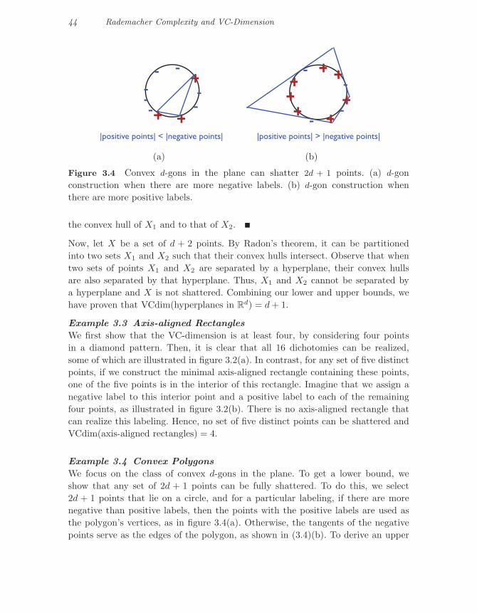
Figure 3.4 Convex d-gons in the plane can shatter 2d + 1 points. (a) d-gonconstruction when there are more negative labels. (b) d-gon construction whenthere are more positive labels.

the convex hull of X1 and to that of X2.

Now, let X be a set of d + 2 points. By Radon’s theorem, it can be partitionedinto two sets X1 and X2 such that their convex hulls intersect. Observe that whentwo sets of points X1 and X2 are separated by a hyperplane, their convex hullsare also separated by that hyperplane. Thus, X1 and X2 cannot be separated bya hyperplane and X is not shattered. Combining our lower and upper bounds, wehave proven that VCdim(hyperplanes in R

d) = d + 1.

Example 3.3 Axis-aligned Rectangles

We first show that the VC-dimension is at least four, by considering four pointsin a diamond pattern. Then, it is clear that all 16 dichotomies can be realized,some of which are illustrated in figure 3.2(a). In contrast, for any set of five distinctpoints, if we construct the minimal axis-aligned rectangle containing these points,one of the five points is in the interior of this rectangle. Imagine that we assign anegative label to this interior point and a positive label to each of the remainingfour points, as illustrated in figure 3.2(b). There is no axis-aligned rectangle thatcan realize this labeling. Hence, no set of five distinct points can be shattered andVCdim(axis-aligned rectangles) = 4.

Example 3.4 Convex Polygons

We focus on the class of convex d-gons in the plane. To get a lower bound, weshow that any set of 2d + 1 points can be fully shattered. To do this, we select2d + 1 points that lie on a circle, and for a particular labeling, if there are morenegative than positive labels, then the points with the positive labels are used asthe polygon’s vertices, as in figure 3.4(a). Otherwise, the tangents of the negativepoints serve as the edges of the polygon, as shown in (3.4)(b). To derive an upper

3.3 VC-dimension 45

sin(

50x)

x

1

-1

10

Figure 3.5 An example of a sine function (with ω = 50) used for classification.

bound, it can be shown that choosing points on the circle maximizes the numberof possible dichotomies, and thus VCdim(convex d-gons) = 2d + 1. Note also thatVCdim(convex polygons) = +∞.

Example 3.5 Sine Functions

The previous examples could suggest that the VC-dimension of H coincides withthe number of free parameters defining H. For example, the number of parametersdefining hyperplanes matches their VC-dimension. However, this does not hold ingeneral. Several of the exercises in this chapter illustrate this fact. The followingprovides a striking example from this point of view. Consider the following familyof sine functions: {t �→ sin(ωt) : ω ∈ R}. One instance of this function class is shownin figure 3.5. These sine functions can be used to classify the points on the real line:a point is labeled positively if it is above the curve, negatively otherwise. Althoughthis family of sine function is defined via a single parameter, ω, it can be shownthat VCdim(sine functions) = +∞ (exercise 3.12).

The VC-dimension of many other hypothesis sets can be determined or upper-bounded in a similar way (see this chapter’s exercises). In particular, the VC-dimension of any vector space of dimension r < ∞ can be shown to be at mostr (exercise 3.11). The next result known as Sauer’s lemma clarifies the connectionbetween the notions of growth function and VC-dimension.

Theorem 3.5 Sauer’s lemmaLet H be a hypothesis set with VCdim(H) = d. Then, for all m ∈ N, the followinginequality holds:

ΠH(m) ≤d∑

i=0

(m

i

). (3.29)


x1 x2 · · · xm−1 xm

· · · · · · · · · · · · · · ·

1 1 0 1 01 1 0 1 10 1 1 1 11 0 0 1 01 0 0 0 1

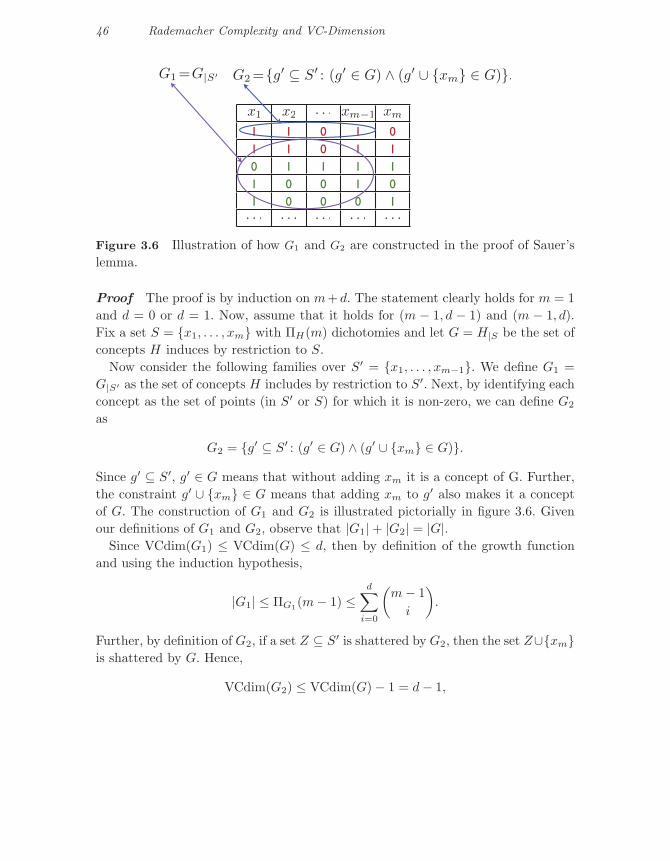
G1 =G|S′ G2 ={g′ ⊆ S′ : (g′ ∈ G) ∧ (g′ ∪ {xm} ∈ G)}.

Figure 3.6 Illustration of how G1 and G2 are constructed in the proof of Sauer’slemma.

Proof The proof is by induction on m+ d. The statement clearly holds for m = 1and d = 0 or d = 1. Now, assume that it holds for (m − 1, d − 1) and (m − 1, d).Fix a set S = {x1, . . . , xm} with ΠH(m) dichotomies and let G = H|S be the set ofconcepts H induces by restriction to S.

Now consider the following families over S′ = {x1, . . . , xm−1}. We define G1 =G|S′ as the set of concepts H includes by restriction to S′. Next, by identifying eachconcept as the set of points (in S′ or S) for which it is non-zero, we can define G2

as

G2 = {g′ ⊆ S′ : (g′ ∈ G) ∧ (g′ ∪ {xm} ∈ G)}.

Since g′ ⊆ S′, g′ ∈ G means that without adding xm it is a concept of G. Further,the constraint g′ ∪ {xm} ∈ G means that adding xm to g′ also makes it a conceptof G. The construction of G1 and G2 is illustrated pictorially in figure 3.6. Givenour definitions of G1 and G2, observe that |G1| + |G2| = |G|.

Since VCdim(G1) ≤ VCdim(G) ≤ d, then by definition of the growth functionand using the induction hypothesis,

|G1| ≤ ΠG1(m − 1) ≤d∑

i=0

(m − 1

i

).

Further, by definition of G2, if a set Z ⊆ S′ is shattered by G2, then the set Z∪{xm}is shattered by G. Hence,

VCdim(G2) ≤ VCdim(G) − 1 = d − 1,

3.3 VC-dimension 47

and by definition of the growth function and using the induction hypothesis,

|G2| ≤ ΠG2(m − 1) ≤d−1∑i=0

(m − 1

i

).

Thus,

|G| = |G1| + |G2| ≤d∑

i=0

(m−1

i

)+

d−1∑i=0

(m−1

i

)=

d∑i=0

(m−1

i

)+(m−1i−1

)=

d∑i=0

(mi

),

which completes the inductive proof.

The significance of Sauer’s lemma can be seen by corollary 3.3, which remarkablyshows that growth function only exhibits two types of behavior: either VCdim(H) =d < +∞, in which case ΠH(m) = O(md), or VCdim(H) = +∞, in which caseΠH(m) = 2m.

Corollary 3.3

Let H be a hypothesis set with VCdim(H) = d. Then for all m ≥ d,

ΠH(m) ≤(em

d

)d

= O(md). (3.30)

Proof The proof begins by using Sauer’s lemma. The first inequality multiplieseach summand by a factor that is greater than or equal to one since m ≥ d, whilethe second inequality adds non-negative summands to the summation.

ΠH(m) ≤d∑

i=0

(m

i

)

≤d∑

i=0

(m

i

)(m

d

)d−i

≤m∑

i=0

(m

i

)(m

d

)d−i

=(m

d

)d m∑i=0

(m

i

)(d

m

)i

=(m

d

)d(

1 +d

m

)m

≤(m

d

)d

ed.

After simplifying the expression using the binomial theorem, the final inequalityfollows using the general identity (1 − x) ≤ e−x.

The explicit relationship just formulated between VC-dimension and the growthfunction combined with corollary 3.2 leads immediately to the following generaliza-


tion bounds based on the VC-dimension.

Corollary 3.4 VC-dimension generalization boundsLet H be a family of functions taking values in {−1, +1} with VC-dimension d.Then, for any δ > 0, with probability at least 1 − δ, the following holds for allh ∈ H:

R(h) ≤ R(h) +

√2d log em

d

m+

√log 1

δ

2m. (3.31)

Thus, the form of this generalization bound is

R(h) ≤ R(h) + O

(√log(m/d)(m/d)

), (3.32)

which emphasizes the importance of the ratio m/d for generalization. The theoremprovides another instance of Occam’s razor principle where simplicity is measuredin terms of smaller VC-dimension.

VC-dimension bounds can be derived directly without using an intermediateRademacher complexity bound, as for (3.25): combining Sauer’s lemma with (3.25)leads to the following high-probability bound

R(h) ≤ R(h) +

√8d log 2em

d + 8 log 4δ

m,

which has the general form of (3.32). The log factor plays only a minor role in thesebounds. A finer analysis can be used in fact to eliminate that factor.

3.4 Lower bounds

In the previous section, we presented several upper bounds on the generalizationerror. In contrast, this section provides lower bounds on the generalization error ofany learning algorithm in terms of the VC-dimension of the hypothesis set used.

These lower bounds are shown by finding for any algorithm a ‘bad’ distribution.Since the learning algorithm is arbitrary, it will be difficult to specify that particulardistribution. Instead, it suffices to prove its existence non-constructively. At a highlevel, the proof technique used to achieve this is the probabilistic method of PaulErdos. In the context of the following proofs, first a lower bound is given on theexpected error over the parameters defining the distributions. From that, the lowerbound is shown to hold for at least one set of parameters, that is one distribution.

3.4 Lower bounds 49

Theorem 3.6 Lower bound, realizable caseLet H be a hypothesis set with VC-dimension d > 1. Then, for any learningalgorithm A, there exist a distribution D over X and a target function f ∈ H

such that

PrS∼Dm

[RD(hS , f) >

d − 132m

]≥ 1/100. (3.33)

Proof Let X = {x0, x1, . . . , xd−1} ⊆ X be a set that is fully shattered by H. Forany ε > 0, we choose D such that its support is reduced to X and so that onepoint (x0) has very high probability (1 − ε), with the rest of the probability massdistributed uniformly among the other points:

PrD

[x0] = 1 − 8ε and ∀i ∈ [1, d − 1], PrD

[xi] =8ε

d − 1. (3.34)

With this definition, most samples would contain x0 and, since X is fully shattered,A can essentially do no better than tossing a coin when determining the label of apoint xi not falling in the training set.

We assume without loss of generality that A makes no error on x0. For a sampleS, we let S denote the set of its elements falling in {x1, . . . , xd−1}, and let S be theset of samples S of size m such that |S| ≤ (d − 1)/2. Now, fix a sample S ∈ S, andconsider the uniform distribution U over all labelings f : X → {0, 1}, which are allin H since the set is shattered. Then, the following lower bound holds:

Ef∼U

[RD(hS , f)] =∑

f

∑x∈X

1h(x) �=f(x) Pr[x] Pr[f ]

≥∑

f

∑x�∈S

1h(x) �=f(x) Pr[x] Pr[f ]

=∑x�∈S

(∑f

1h(x) �=f(x) Pr[f ])

Pr[x]

=12

∑x�∈S

Pr[x] ≥ 12

d − 12

8ε

d − 1= 2ε. (3.35)

The first lower bound holds because we remove non-negative terms from thesummation when we only consider x �∈ S instead of all x in X. After rearrangingterms, the subsequent equality holds since we are taking an expectation over f ∈ H

with uniform weight on each f and H shatters X. The final lower bound holds dueto the definitions of D and S, the latter which implies that |X − S| ≥ (d − 1)/2.

Since (3.35) holds for all S ∈ S, it also holds in expectation over all S ∈ S:ES∈S

[Ef∼U [RD(hS , f)]

] ≥ 2ε. By Fubini’s theorem, the expectations can be


permuted, thus,

Ef∼U

[E

S∈S[RD(hS , f)]

]≥ 2ε. (3.36)

This implies that ES∈S [RD(hS , f0)] ≥ 2ε for at least one labeling f0 ∈ H. Decom-posing this expectation into two parts and using RD(hS , f0) ≤ PrD[X − {x0}], weobtain:

ES∈S

[RD(hS , f0)] =∑

S :RD(hS ,f0)≥ε

RD(hS , f0) Pr[RD(hS , f0)] +∑

S :RD(hS ,f0)<ε

RD(hS , f0) Pr[RD(hS , f0)]

≤ PrD

[X − {x0}] PrS∈S

[RD(hS , f0) ≥ ε] + ε PrS∈S

[RD(hS , f0) < ε]

≤ 8ε PrS∈S

[RD(hS , f0) ≥ ε] + ε(1 − Pr

S∈S[RD(hS , f0) ≥ ε]

).

Collecting terms in PrS∈S [RD(hS , f0) ≥ ε] yields

PrS∈S

[RD(hS , f0) ≥ ε] ≥ 17ε

(2ε − ε) =17. (3.37)

Thus, the probability over all samples S (not necessarily in S) can be lower boundedas

PrS

[RD(hS , f0) ≥ ε] ≥ PrS∈S

[RD(hS , f0) ≥ ε] Pr[S] ≥ 17

Pr[S]. (3.38)

This leads us to find a lower bound for Pr[S]. The probability that more than(d−1)/2 points are drawn in a sample of size m verifies the Chernoff bound for anyγ > 0:

1 − Pr[S] = Pr[Sm ≥ 8εm(1 + γ)] ≤ e−8εm γ2

3 . (3.39)

Therefore, for ε = (d − 1)/(32m) and γ = 1,

Pr[Sm ≥ d−12 ] ≤ e−(d−1)/12 ≤ e−1/12 ≤ 1 − 7δ, (3.40)

for δ ≤ .01. Thus Pr[S] ≥ 7δ and PrS [RD(hS , f0) ≥ ε] ≥ δ.

The theorem shows that for any algorithm A, there exists a ‘bad’ distribution overX and a target function f for which the error of the hypothesis returned by A isΩ( d

m ) with some constant probability. This further demonstrates the key role playedby the VC-dimension in learning. The result implies in particular that PAC-learningin the non-realizable case is not possible when the VC-dimension is infinite.

Note that the proof shows a stronger result than the statement of the theorem:the distribution D is selected independently of the algorithm A. We now present atheorem giving a lower bound in the non-realizable case. The following two lemmaswill be needed for the proof.

3.4 Lower bounds 51

Lemma 3.2

Let α be a uniformly distributed random variable taking values in {α−, α+}, whereα− = 1

2 − ε2 and α+ = 1

2 + ε2 , and let S be a sample of m ≥ 1 random variables

X1, . . . , Xm taking values in {0, 1} and drawn i.i.d. according to the distribution Dα

defined by PrDα[X = 1] = α. Let h be a function from Xm to {α−, α+}, then the

following holds:

Eα

[Pr

S∼Dmα

[h(S) �= α]]≥ Φ(2�m/2�, ε), (3.41)

where Φ(m, ε) = 14

(1 −

√1 − exp

(− mε2

1−ε2

))for all m and ε.

Proof The lemma can be interpreted in terms of an experiment with two coinswith biases α− and α+. It implies that for a discriminant rule h(S) based on asample S drawn from Dα− or Dα+ , to determine which coin was tossed, the samplesize m must be at least Ω(1/ε2). The proof is left as an exercise (exercise 3.19).

We will make use of the fact that for any fixed ε the function m �→ Φ(m,x) isconvex, which is not hard to establish.

Lemma 3.3

Let Z be a random variable taking values in [0, 1]. Then, for any γ ∈ [0, 1),

Pr[z > γ] ≥ E[Z] − γ

1 − γ> E[Z] − γ. (3.42)

Proof Since the values taken by Z are in [0, 1],

E[Z] =∑z≤γ

Pr[Z = z]z +∑z>γ

Pr[Z = z]z

≤∑z≤γ

Pr[Z = z]γ +∑z>γ

Pr[Z = z]

= γ Pr[Z ≤ γ] + Pr[Z > γ]

= γ(1 − Pr[Z > γ]) + Pr[Z > γ]

= (1 − γ) Pr[Z > γ] + γ,

which concludes the proof.

Theorem 3.7 Lower bound, non-realizable caseLet H be a hypothesis set with VC-dimension d > 1. Then, for any learningalgorithm A, there exists a distribution D over X × {0, 1} such that:

PrS∼Dm

[RD(hS) − inf

h∈HRD(h) >

√d

320m

]≥ 1/64. (3.43)


Equivalently, for any learning algorithm, the sample complexity verifies

m ≥ d

320ε2. (3.44)

Proof Let X = {x1, x1, . . . , xd} ⊆ X be a set fully shattered by H. For anyα ∈ [0, 1] and any vector σ = (σ1, . . . , σd)� ∈ {−1, +1}d, we define a distributionDσ with support X × {0, 1} as follows:

∀i ∈ [1, d], PrDσ

[(xi, 1)] =1d

(12

+σiα

2

). (3.45)

Thus, the label of each point xi, i ∈ [1, d], follows the distribution PrDσ [·|xi], thatof a biased coin where the bias is determined by the sign of σi and the magnitudeof α. To determine the most likely label of each point xi, the learning algorithmwill therefore need to estimate PrDσ

[1|xi] with an accuracy better than α. To makethis further difficult, α and σ will be selected based on the algorithm, requiring, asin lemma 3.2, Ω(1/α2) instances of each point xi in the training sample.

Clearly, the Bayes classifier h∗Dσ

is defined by h∗Dσ

(xi) = argmaxy∈{0,1} Pr[y|xi] =1σi>0 for all i ∈ [1, d]. h∗

Dσis in H since X is fully shattered. For all h ∈ H,

RDσ (h) − RDσ (h∗Dσ

) =1d

∑x∈X

(α

2+

α

2

)1h(x) �=h∗

Dσ(x) =

α

d

∑x∈X

1h(x) �=h∗Dσ

(x). (3.46)

Let hS denote the hypothesis returned by the learning algorithm A after receivinga labeled sample S drawn according to Dσ. We will denote by |S|x the number ofoccurrences of a point x in S. Let U denote the uniform distribution over {−1, +1}d.

3.4 Lower bounds 53

Then, in view of (3.46), the following holds:

Eσ∼US∼Dm

σ

[1α

[RDσ

(hS) − RDσ(h∗

Dσ)]]

=1d

∑x∈X

Eσ∼US∼Dm

σ

[1hS(x) �=h∗

Dσ(x)

]=

1d

∑x∈X

Eσ∼U

[Pr

S∼Dmσ

[hS(x) �= h∗

Dσ(x)]]

=1d

∑x∈X

m∑n=0

Eσ∼U

[Pr

S∼Dmσ

[hS(x) �= h∗

Dσ(x)

∣∣ |S|x = n]Pr[|S|x = n]

]≥ 1

d

∑x∈X

m∑n=0

Φ(n + 1, α) Pr[|S|x = n] (lemma 3.2)

≥ 1d

∑x∈X

Φ(m/d + 1, α) (convexity of Φ(·, α) and Jensen’s ineq.)

= Φ(m/d + 1, α).

Since the expectation over σ is lower-bounded by Φ(m/d + 1, α), there must existsome σ ∈ {−1, +1}d for which

ES∼Dm

σ

[1α

[RDσ

(hS) − RDσ(h∗

Dσ)]]

> Φ(m/d + 1, α). (3.47)

Then, by lemma 3.3, for that σ, for any γ ∈ [0, 1],

PrS∼Dm

σ

[1α

[RDσ

(hS) − RDσ(h∗

Dσ)]

> γu

]> (1 − γ)u, (3.48)

where u = Φ(m/d + 1, α). Selecting δ and ε such that δ ≤ (1 − γ)u and ε ≤ γαu

gives

PrS∼Dm

σ

[RDσ

(hS) − RDσ(h∗

Dσ) > ε

]> δ. (3.49)


To satisfy the inequalities defining ε and δ, let γ = 1 − 8δ. Then,

δ ≤ (1 − γ)u ⇐⇒ u ≥ 18

(3.50)

⇐⇒ 14

(1 −

√1 − exp

(− (m/d + 1)α2

1 − α2

))≥ 1

8(3.51)

⇐⇒ (m/d + 1)α2

1 − α2≤ log

43

(3.52)

⇐⇒ m

d≤ (

1α2

− 1) log43

− 1. (3.53)

Selecting α = 8ε/(1 − 8δ) gives ε = γα/8 and the condition

m

d≤(

(1 − 8δ)2

64ε2− 1

)log

43

− 1. (3.54)

Let f(1/ε2) denote the right-hand side. We are seeking a sufficient condition of theform m/d ≤ ω/ε2. Since ε ≤ 1/64, to ensure that ω/ε2 ≤ f(1/ε2), it suffices toimpose ω/(1/64)2 = f(1/(1/64)2). This condition gives

ω = (7/64)2 log(4/3) − (1/64)2(log(4/3) + 1) ≈ .003127 ≥ 1/320 = .003125.

Thus, ε2 ≤ 1320(m/d) is sufficient to ensure the inequalities.

The theorem shows that for any algorithm A, in the non-realizable case, there existsa ‘bad’ distribution over X × {0, 1} such that the error of the hypothesis returnedby A is Ω

(√dm

)with some constant probability. The VC-dimension appears as a

critical quantity in learning in this general setting as well. In particular, with aninfinite VC-dimension, agnostic PAC-learning is not possible.

3.5 Chapter notes

The use of Rademacher complexity for deriving generalization bounds in learningwas first advocated by Koltchinskii [2001], Koltchinskii and Panchenko [2000], andBartlett, Boucheron, and Lugosi [2002a], see also [Koltchinskii and Panchenko,2002, Bartlett and Mendelson, 2002]. Bartlett, Bousquet, and Mendelson [2002b]introduced the notion of local Rademacher complexity , that is the Rademachercomplexity restricted to a subset of the hypothesis set limited by a bound onthe variance. This can be used to derive better guarantees under some regularityassumptions about the noise.

Theorem 3.3 is due to Massart [2000]. The notion of VC-dimension was introducedby Vapnik and Chervonenkis [1971] and has been since extensively studied [Vapnik,

3.6 Exercises 55

2006, Vapnik and Chervonenkis, 1974, Blumer et al., 1989, Assouad, 1983, Dudley,1999]. In addition to the key role it plays in machine learning, the VC-dimension isalso widely used in a variety of other areas of computer science and mathematics(e.g., see Shelah [1972], Chazelle [2000]). Theorem 3.5 is known as Sauer’s lemmain the learning community, however the result was first given by Vapnik andChervonenkis [1971] (in a somewhat different version) and later independently bySauer [1972] and Shelah [1972].

In the realizable case, lower bounds for the expected error in terms of the VC-dimension were given by Vapnik and Chervonenkis [1974] and Haussler et al. [1988].Later, a lower bound for the probability of error such as that of theorem 3.6 wasgiven by Blumer et al. [1989]. Theorem 3.6 and its proof, which improves uponthis previous result, are due to Ehrenfeucht, Haussler, Kearns, and Valiant [1988].Devroye and Lugosi [1995] gave slightly tighter bounds for the same problem witha more complex expression. Theorem 3.7 giving a lower bound in the non-realizablecase and the proof presented are due to Anthony and Bartlett [1999]. For otherexamples of application of the probabilistic method demonstrating its full power,consult the reference book of Alon and Spencer [1992].

There are several other measures of the complexity of a family of functions usedin machine learning, including covering numbers, packing numbers, and some othercomplexity measures discussed in chapter 10. A covering number Np(G, ε) is theminimal number of Lp balls of radius ε > 0 needed to cover a family of loss functionsG. A packing number Mp(G, ε) is the maximum number of non-overlapping Lp

balls of radius ε centered in G. The two notions are closely related, in particularit can be shown straightfowardly that Mp(G, 2ε) ≤ Np(G, ε) ≤ Mp(G, ε) for G

and ε > 0. Each complexity measure naturally induces a different reduction ofinfinite hypothesis sets to finite ones, thereby resulting in generalization boundsfor infinite hypothesis sets. Exercise 3.22 illustrates the use of covering numbersfor deriving generalization bounds using a very simple proof. There are also closerelationships between these complexity measures: for example, by Dudley’s theorem,the empirical Rademacher complexity can be bounded in terms of N2(G, ε) [Dudley,1967, 1987] and the covering and packing numbers can be bounded in terms of theVC-dimension [Haussler, 1995]. See also [Ledoux and Talagrand, 1991, Alon et al.,1997, Anthony and Bartlett, 1999, Cucker and Smale, 2001, Vidyasagar, 1997] fora number of upper bounds on the covering number in terms of other complexitymeasures.

3.6 Exercises

3.1 Growth function of intervals in R. Let H be the set of intervals in R. The VC-dimension of H is 2. Compute its shattering coefficient ΠH(m), m ≥ 0. Compare


your result with the general bound for growth functions.

3.2 Lower bound on growth function. Prove that Sauer’s lemma (theorem 3.5) istight, i.e., for any set X of m > d elements, show that there exists a hypothesisclass H of VC-dimension d such that ΠH(m) =

∑di=0

(mi

).

3.3 Singleton hypothesis class. Consider the trivial hypothesis set H = {h0}.

(a) Show that Rm(H) = 0 for any m > 0.

(b) Use a similar construction to show that Massart’s lemma (theorem 3.3) istight.

3.4 Rademacher identities. Fix m ≥ 1. Prove the following identities for any α ∈ R

and any two hypothesis sets H and H ′ of functions mapping from X to R:

(a) Rm(αH) = |α|Rm(H).

(b) Rm(H + H ′) = Rm(H) + Rm(H ′).

(c) Rm({max(h, h′) : h ∈ H,h′ ∈ H ′}),where max(h, h′) denotes the function x �→ maxx∈X (h(x), h′(x)) (Hint : youcould use the identity max(a, b) = 1

2 [a + b + |a − b|] valid for all a, b ∈ R andTalagrand’s contraction lemma (see lemma 4.2)).

3.5 Rademacher complexity. Professor Jesetoo claims to have found a better boundon the Rademacher complexity of any hypothesis set H of functions taking valuesin {−1, +1}, in terms of its VC-dimension VCdim(H). His bound is of the formRm(H) ≤ O

(VCdim(H)m

). Can you show that Professor Jesetoo’s claim cannot be

correct? (Hint : consider a hypothesis set H reduced to just two simple functions.)

3.6 VC-dimension of union of k intervals. What is the VC-dimension of subsets ofthe real line formed by the union of k intervals?

3.7 VC-dimension of finite hypothesis sets. Show that the VC-dimension of a finitehypothesis set H is at most log2 |H|.

3.8 VC-dimension of subsets. What is the VC-dimension of the set of subsets Iα ofthe real line parameterized by a single parameter α: Iα = [α, α + 1] ∪ [α + 2, +∞)?

3.9 VC-dimension of closed balls in Rn. Show that the VC-dimension of the set

of all closed balls in Rn, i.e., sets of the form {x ∈ R

n : ‖x − x0‖2 ≤ r} for somex0 ∈ R

n and r ≥ 0, is less than or equal to n + 2.

3.6 Exercises 57

3.10 VC-dimension of ellipsoids. What is the VC-dimension of the set of all ellipsoidsin R

n?

3.11 VC-dimension of a vector space of real functions. Let F be a finite-dimensionalvector space of real functions on R

n, dim(F ) = r < ∞. Let H be the set ofhypotheses:

H = {{x : f(x) ≥ 0} : f ∈ F}.

Show that d, the VC-dimension of H, is finite and that d ≤ r. (Hint : select anarbitrary set of m = r + 1 points and consider linear mapping u : F → R

m definedby: u(f) = (f(x1), . . . , f(xm)).)

3.12 VC-dimension of sine functions. Consider the hypothesis family of sine func-tions (Example 3.5): {x → sin(ωx) : ω ∈ R} .

(a) Show that for any x ∈ R the points x, 2x, 3x and 4x cannot be shatteredby this family of sine functions.

(b) Show that the VC-dimension of the family of sine functions is infinite.(Hint : show that {2−m : m ∈ N} can be fully shattered for any m > 0.)

3.13 VC-dimension of union of halfspaces. Determine the VC-dimension of thesubsets of the real line formed by the union of k intervals.

3.14 VC-dimension of intersection of halfspaces. Consider the class Ck of convexintersections of k halfspaces. Give lower and upper bound estimates for VCdim(Ck).

3.15 VC-dimension of intersection concepts.

(a) Let C1 and C2 be two concept classes. Show that for any concept classC = {c1 ∩ c2 : c1 ∈ C1, c2 ∈ C2},

ΠC(m) ≤ ΠC1(m) ΠC2(m). (3.55)

(b) Let C be a concept class with VC-dimension d and let Cs be the conceptclass formed by all intersections of s concepts from C, s ≥ 1. Show that theVC-dimension of Cs is bounded by 2ds log2(3s). (Hint : show that log2(3x) <

9x/(2e) for any x ≥ 2.)

3.16 VC-dimension of union of concepts. Let A and B be two sets of functionsmapping from X into {0, 1}, and assume that both A and B have finite VC-dimension, with VCdim(A) = dA and VCdim(B) = dB . Let C = A ∪ B be the


union of A and B.

(a) Prove that for all m, ΠC(m) ≤ ΠA(m) + ΠB(m).

(b) Use Sauer’s lemma to show that for m ≥ dA + dB + 2, ΠC(m) < 2m, andgive a bound on the VC-dimension of C.

3.17 VC-dimension of symmetric difference of concepts. For two sets A and B, letAΔB denote the symmetric difference of A and B, i.e., AΔB = (A∪B)− (A∩B).Let H be a non-empty family of subsets of X with finite VC-dimension. Let A bean element of H and define HΔA = {XΔA : X ∈ H}. Show that

VCdim(HΔA) = VCdim(H).

3.18 Symmetric functions. A function h : {0, 1}n → {0, 1} is symmetric if its valueis uniquely determined by the number of 1’s in the input. Let C denote the set ofall symmetric functions.

(a) Determine the VC-dimension of C.

(b) Give lower and upper bounds on the sample complexity of any consistentPAC learning algorithm for C.

(c) Note that any hypothesis h ∈ C can be represented by a vector (y0, y1, ..., yn) ∈{0, 1}n+1, where yi is the value of h on examples having precisely i 1’s. Devisea consistent learning algorithm for C based on this representation.

3.19 Biased coins. Professor Moent has two coins in his pocket, coin xA and coinxB . Both coins are slightly biased, i.e., Pr[xA = 0] = 1/2 − ε/2 and Pr[xB = 0] =1/2 + ε/2, where 0 < ε < 1 is a small positive number, 0 denotes heads and 1denotes tails. He likes to play the following game with his students. He picks a coinx ∈ {xA, xB} from his pocket uniformly at random, tosses it m times, reveals thesequence of 0s and 1s he obtained and asks which coin was tossed. Determine howlarge m needs to be for a student’s coin prediction error to be at most δ > 0.

(a) Let S be a sample of size m. Professor Moent’s best student, Oskar, playsaccording to the decision rule fo : {0, 1}m → {xA, xB} defined by fo(S) = xA

iff N(S) < m/2, where N(S) is the number of 0’s in sample S.Suppose m is even, then show that

error(fo) ≥ 12

Pr[N(S) ≥ m

2

∣∣∣x = xA

]. (3.56)

(b) Assuming m even, use the inequalities given in the appendix (section D.3)

3.6 Exercises 59

to show that

error(fo) >14

[1 −

[1 − e

− mε2

1−ε2

] 12]. (3.57)

(c) Argue that if m is odd, the probability can be lower bounded by usingm + 1 in the bound in (a) and conclude that for both odd and even m,

error(fo) >14

[1 −

[1 − e

− 2�m/2�ε2

1−ε2

] 12]. (3.58)

(d) Using this bound, how large must m be if Oskar’s error is at most δ, where0 < δ < 1/4. What is the asymptotic behavior of this lower bound as a functionof ε?

(e) Show that no decision rule f : {0, 1}m → {xa, xB} can do better thanOskar’s rule fo. Conclude that the lower bound of the previous question appliesto all rules.

3.20 Infinite VC-dimension.

(a) Show that if a concept class C has infinite VC-dimension, then it is notPAC-learnable.

(b) In the standard PAC-learning scenario, the learning algorithm receives allexamples first and then computes its hypothesis. Within that setting, PAC-learning of concept classes with infinite VC-dimension is not possible as seenin the previous question.Imagine now a different scenario where the learning algorithm can alternatebetween drawing more examples and computation. The objective of this prob-lem is to prove that PAC-learning can then be possible for some concept classeswith infinite VC-dimension.Consider for example the special case of the concept class C of all subsets ofnatural numbers. Professor Vitres has an idea for the first stage of a learningalgorithm L PAC-learning C. In the first stage, L draws a sufficient number ofpoints m such that the probability of drawing a point beyond the maximumvalue M observed be small with high confidence. Can you complete ProfessorVitres’ idea by describing the second stage of the algorithm so that it PAC-learns C? The description should be augmented with the proof that L canPAC-learn C.

3.21 VC-dimension generalization bound – realizable case. In this exercise we showthat the bound given in corollary 3.4 can be improved to O(d log(m/d)

m ) in therealizable setting. Assume we are in the realizable scenario, i.e. the target concept isincluded in our hypothesis class H. We will show that if a hypothesis h is consistent


with a sample S ∼ Dm then for any ε > 0 such that mε ≥ 8

Pr[R(h) > ε] ≤ 2[2em

d

]d2−mε/2 . (3.59)

(a) Let HS ⊆ H be the subset of hypotheses consistent with the sample S,let RS(h) denote the empirical error with respect to the sample S and defineS′ as a another independent sample drawn from Dm. Show that the followinginequality holds for any h0 ∈ HS :

Pr[

suph∈HS

|RS(h) − RS′(h)| >ε

2

]≥ Pr

[B[m, ε] >

mε

2

]Pr[R(h0) > ε] ,

where B[m, ε] is a binomial random variable with parameters [m, ε]. (Hint :prove and use the fact that Pr[R(h) ≥ ε

2 ] ≥ Pr[R(h) > ε2 ∧ R(h) > ε].)

(b) Prove that Pr[B(m, ε) > mε

2

]≥ 1

2 . Use this inequality along with theresult from (a) to show that for any h0 ∈ HS

Pr[R(h0) > ε

]≤ 2 Pr

[sup

h∈HS

|RS(h) − RS′(h)| >ε

2

].

(c) Instead of drawing two samples, we can draw one sample T of size 2m thenuniformly at random split it into S and S′. The right hand side of part (b) canthen be rewritten as:

Pr[

suph∈HS

|RS(h)−RS′(h)| >ε

2

]= Pr

T∼D2m:T→[S,S′]

[∃h∈H : RS(h) = 0 ∧ RS′(h) >

ε

2

].

Let h0 be a hypothesis such that RT (h0) > ε2 and let l > mε

2 be the totalnumber of errors h0 makes on T . Show that the probability of all l errorsfalling into S′ is upper bounded by 2−l.

(d) Part (b) implies that for any h ∈ H

PrT∼D2m:T→(S,S′)

[RS(h) = 0 ∧ RS′(h) >

ε

2

∣∣∣ RT (h0) >ε

2

]≤ 2−l .

Use this bound to show that for any h ∈ H

PrT∼D2m:T→(S,S′)

[RS(h) = 0 ∧ RS′(h) >

ε

2

]≤ 2−

εm2 .

(e) Complete the proof of inequality (3.59) by using the union bound to upperbound Pr T∼D2m:

T→(S,S′)

[∃h∈H : RS(h) = 0 ∧ RS′(h) > ε

2

]. Show that we can achieve

a high probability generalization bound that is of the order O(d log(m/d)m ).

3.6 Exercises 61

3.22 Generalization bound based on covering numbers. Let H be a family offunctions mapping X to a subset of real numbers Y ⊆ R. For any ε > 0, thecovering number N (H, ε) of H for the L∞ norm is the minimal k ∈ N such that H

can be covered with k balls of radius ε, that is, there exists {h1, . . . , hk} ⊆ H suchthat, for all h ∈ H, there exists i ≤ k with ‖h − hi‖∞ = maxx∈X |h(x) − hi(x)| ≤ ε.In particular, when H is a compact set, a finite covering can be extracted from acovering of H with balls of radius ε and thus N (H, ε) is finite.

Covering numbers provide a measure of the complexity of a class of functions: thelarger the covering number, the richer is the family of functions. The objective ofthis problem is to illustrate this by proving a learning bound in the case of thesquared loss. Let D denote a distribution over X × Y according to which labeledexamples are drawn. Then, the generalization error of h ∈ H for the squared loss isdefined by R(h) = E(x,y)∼D[(h(x)−y)2] and its empirical error for a labeled sampleS = ((x1, y1), . . . , (xm, ym)) by R(h) = 1

m

∑mi=1(h(xi)−yi)2. We will assume that H

is bounded, that is there exists M > 0 such that |h(x)−y| ≤ M for all (x, y) ∈ X×Y.The following is the generalization bound proven in this problem:

PrS∼Dm

[suph∈H

|R(h) − R(h)| ≥ ε]≤ N

(H,

ε

8M

)2 exp

(−mε2

2M4

). (3.60)

The proof is based on the following steps.

(a) Let LS = R(h) − R(h), then show that for all h1, h2 ∈ H and any labeledsample S, the following inequality holds:

|LS(h1) − LS(h2)| ≤ 4M‖h1 − h2‖∞ .

(b) Assume that H can be covered by k subsets B1, . . . , Bk, that is H =B1 ∪ . . .∪Bk. Then, show that, for any ε > 0, the following upper bound holds:

PrS∼Dm

[suph∈H

|LS(h)| ≥ ε]≤

k∑i=1

PrS∼Dm

[suph∈Bi

|LS(h)| ≥ ε].

(c) Finally, let k = N (H, ε8M ) and let B1, . . . , Bk be balls of radius ε/(8M)

centered at h1, . . . , hk covering H. Use part (a) to show that for all i ∈ [1, k],

PrS∼Dm

[suph∈Bi

|LS(h)| ≥ ε]≤ Pr

S∼Dm

[|LS(hi)| ≥ ε

2

],

and apply Hoeffding’s inequality (theorem D.1) to prove (3.60).

3 Rademacher Complexity and VC- Dimension

Documents

Transcript of 3 Rademacher Complexity and VC- Dimension