
3 Mapping of Spatial Data - ifis.cs.tu-bs.de · 3.1 Properties of Maps 3.2 Signatures, Text, Color...
132
3.1 Properties of Maps 3.2 Signatures, Text, Color 3.3 Geometric Generalization 3.4 Label and Symbol Placement 3.5 Summary Spatial Databases and GIS – Karl Neumann, Sarah Tauscher– Ifis – TU Braunschweig 214 3 Mapping of Spatial Data http://homepage.univie.ac.at/.../Janschitz_Text.pdf
Transcript of 3 Mapping of Spatial Data - ifis.cs.tu-bs.de · 3.1 Properties of Maps 3.2 Signatures, Text, Color...

3.1 Properties of Maps
3.2 Signatures, Text, Color
3.3 Geometric Generalization
3.4 Label and Symbol
Placement
3.5 Summary
Spatial Databases and GIS – Karl Neumann, Sarah Tauscher– Ifis – TU Braunschweig 214
3 Mapping of Spatial Data
http://homepage.univie.ac.at/.../Janschitz_Text.pdf
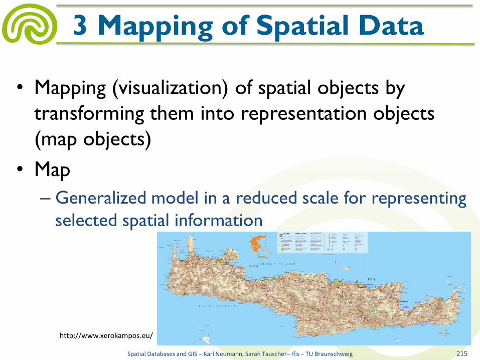
• Mapping (visualization) of spatial objects by
transforming them into representation objects
(map objects)
• Map
– Generalized model in a reduced scale for representing
selected spatial information
Spatial Databases and GIS – Karl Neumann, Sarah Tauscher– Ifis – TU Braunschweig 215
3 Mapping of Spatial Data
http://www.xerokampos.eu/

• Topographic map
– Geometrically and positionally accurate representation of landscape objects drawn to scale (topography, water network, land use, transportation routes)
Spatial Databases and GIS – Karl Neumann, Sarah Tauscher– Ifis – TU Braunschweig 216
3 Mapping of Spatial Data
http://www.wiedenbruegge.net/

• Thematic map
– Emphasis is
on subject-
specific
information
(geological
map,
vegetation
map, biotope
map)
Spatial Databases and GIS – Karl Neumann, Sarah Tauscher– Ifis – TU Braunschweig 217
3 Mapping of Spatial Data
htt
p:/
/ww
w.lb
eg.n
ied
ersa
chse
n.d
e/
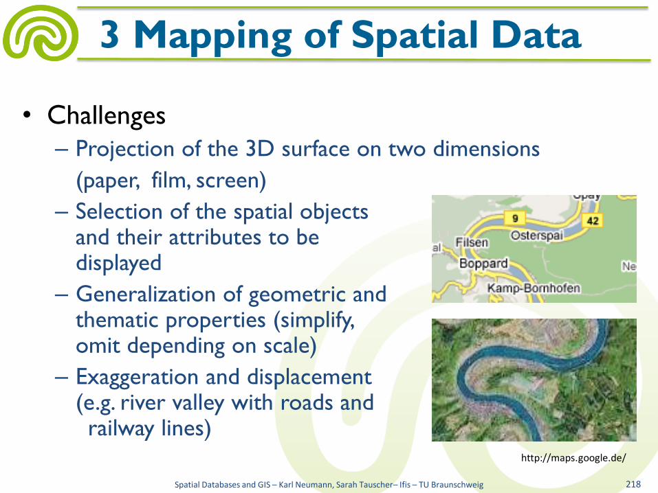
• Challenges
– Projection of the 3D surface on two dimensions
(paper, film, screen)
– Selection of the spatial objects and their attributes to be displayed
– Generalization of geometric and thematic properties (simplify, omit depending on scale)
– Exaggeration and displacement (e.g. river valley with roads and railway lines)
Spatial Databases and GIS – Karl Neumann, Sarah Tauscher– Ifis – TU Braunschweig 218
3 Mapping of Spatial Data
http://maps.google.de/

• Graticule
– Mapping the earth (sphere,
ellipsoid) to a plane
– Two tasks
• Conversion of geographic
coordinates (longitude
and latitude) to cartesian
coordinates (x, y; easting,
northing)
• Scaling of the map
Spatial Databases and GIS – Karl Neumann, Sarah Tauscher– Ifis – TU Braunschweig 219
3.1 Properties of Maps
www.klett.de
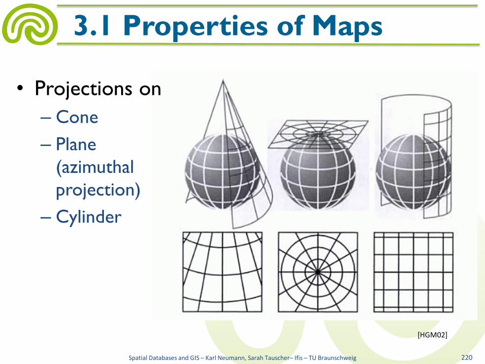
• Projections on
– Cone
– Plane
(azimuthal
projection)
– Cylinder
Spatial Databases and GIS – Karl Neumann, Sarah Tauscher– Ifis – TU Braunschweig 220
3.1 Properties of Maps
[HGM02]
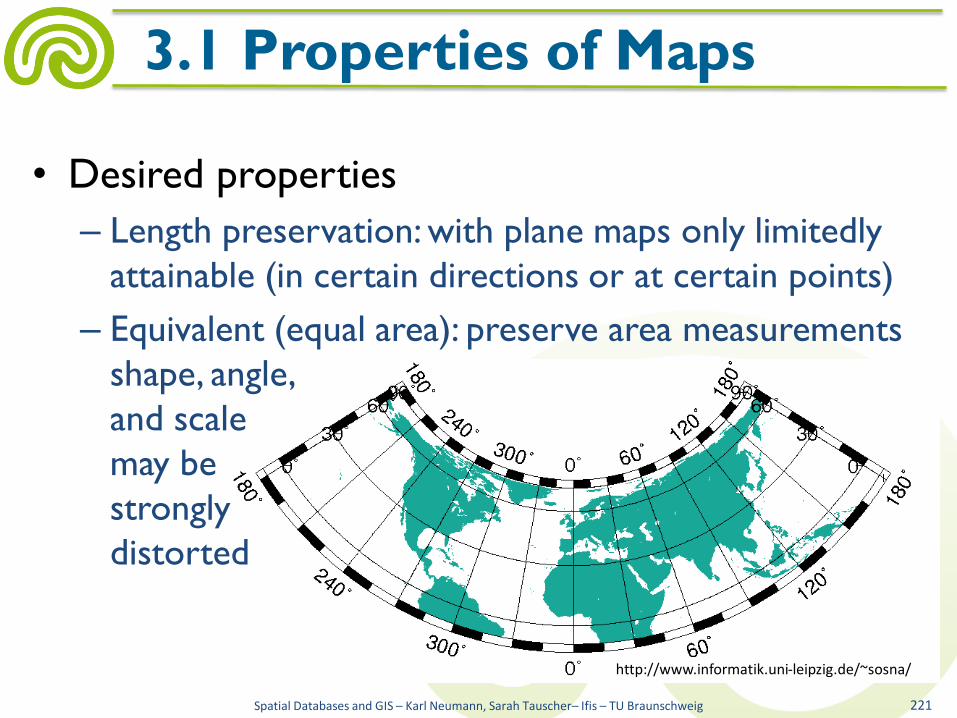
• Desired properties
– Length preservation: with plane maps only limitedly
attainable (in certain directions or at certain points)
– Equivalent (equal area): preserve area measurements
shape, angle,
and scale
may be
strongly
distorted
Spatial Databases and GIS – Karl Neumann, Sarah Tauscher– Ifis – TU Braunschweig 221
3.1 Properties of Maps
http://www.informatik.uni-leipzig.de/~sosna/
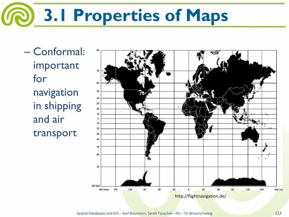
– Conformal:
important
for
navigation
in shipping
and air
transport
Spatial Databases and GIS – Karl Neumann, Sarah Tauscher– Ifis – TU Braunschweig 222
3.1 Properties of Maps
http://flightnavigation.de/

• Areas and angles can not be preserved at the
same time, therefore
– Compromise projections minimize overall distortion
Spatial Databases and GIS – Karl Neumann, Sarah Tauscher– Ifis – TU Braunschweig 223
3.1 Properties of Maps
htt
p:/
/su
pp
ort
2.d
un
das
.co
m/O
nlin
eDo
cum
enta
tio
n/
Web
Map
2005
/Map
Pro
ject
ion
s.h
tml

• The Gauss-Krüger coordinate system
– Used in Germany and Austria
– Cartesian coordinate system to represent small areas
– Divides the surface of the earth into zones
• Each 3° of longitude in width
• The zones are projected onto a cylinder with the earths
diameter
Spatial Databases and GIS – Karl Neumann, Sarah Tauscher– Ifis – TU Braunschweig 224
3.1 Properties of Maps
www.geogr.uni-jena.de/.../GEO142_3b.ppt http://homepage.univie.ac.at/.../Janschitz_Text.pdf
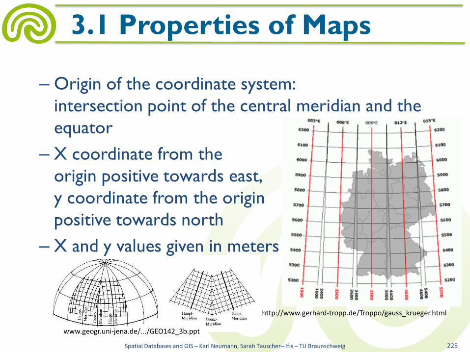
– Origin of the coordinate system:
intersection point of the central meridian and the
equator
– X coordinate from the
origin positive towards east,
y coordinate from the origin
positive towards north
– X and y values given in meters
Spatial Databases and GIS – Karl Neumann, Sarah Tauscher– Ifis – TU Braunschweig 225
3.1 Properties of Maps
http://www.gerhard-tropp.de/Troppo/gauss_krueger.html
www.geogr.uni-jena.de/.../GEO142_3b.ppt

– To avoid negative x coordinates the central meridian
is set to 500,000 m (false easting)
– Each projection zone (3°, 6°, ..., 177°) is identified
by a number (1, 2, …, 59)
– This number is placed prior to the x value
– Example: the Gauss-Krüger coordinates
x: 3,567,780.339 and y: 5,929,989.731
refer to the following location
x: 67,780.339 m East of the 9° meridian
y: 5,929,989.731 m North of the equator
Spatial Databases and GIS – Karl Neumann, Sarah Tauscher– Ifis – TU Braunschweig 226
3.1 Properties of Maps

• Transforming geographic coordinates into
Gauss-Krüger coordinates
– Given geographic coordinates lon, lat
(e.g. from GPS, reference ellipsoid: World Geodetic
System 1984 (WGS 84))
– Transformation into
Cartesian coordinates x, y, z
Spatial Databases and GIS – Karl Neumann, Sarah Tauscher– Ifis – TU Braunschweig 227
3.1 Properties of Maps
https://www.univie.ac.at/
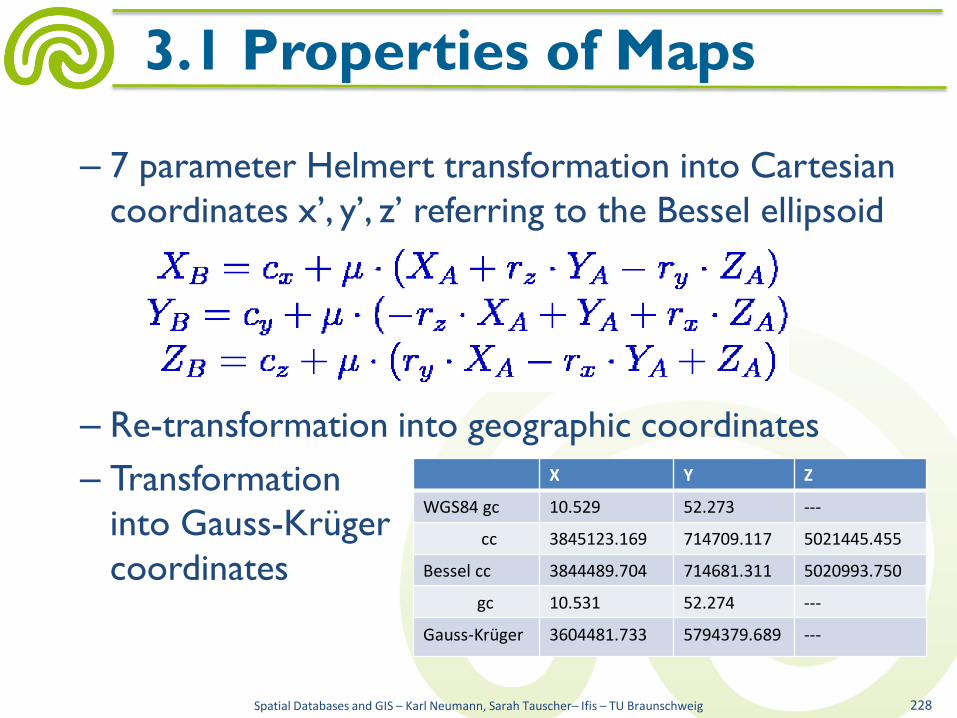
– 7 parameter Helmert transformation into Cartesian
coordinates x’, y’, z’ referring to the Bessel ellipsoid
– Re-transformation into geographic coordinates
– Transformation
into Gauss-Krüger
coordinates
Spatial Databases and GIS – Karl Neumann, Sarah Tauscher– Ifis – TU Braunschweig 228
3.1 Properties of Maps
X Y Z
WGS84 gc 10.529 52.273 ---
cc 3845123.169 714709.117 5021445.455
Bessel cc 3844489.704 714681.311 5020993.750
gc 10.531 52.274 ---
Gauss-Krüger 3604481.733 5794379.689 ---

• The UTM coordinate system
– Similar to the Gauss-Krüger
system
– Divides the surface of the
earth into 6° zones
– Covers the area
between 84° North
and 80° South
Spatial Databases and GIS – Karl Neumann, Sarah Tauscher– Ifis – TU Braunschweig 229
3.1 Properties of Maps
https://www.e-education.psu.edu/
http://earth-info.nga.mil/

– The diameter of the
transverse cylinder is
slightly smaller than the
diameter of the Earth
secant projection with
two lines of true scale
(about 180 km on each
side of the central
meridian)
Spatial Databases and GIS – Karl Neumann, Sarah Tauscher– Ifis – TU Braunschweig 230
3.1 Properties of Maps
https://www.e-education.psu.edu/

• Common mapping errors
Spatial Databases and GIS – Karl Neumann, Sarah Tauscher– Ifis – TU Braunschweig 231
3.1 Properties of Maps
interchanging of x- and y-coordinates
no trans-formation into Cartesian coordinates
ignoring the negative direction of the canvas` y-axis

• Structure of maps
– Body of the map presentation of the actual map
– Map margin contains name, map, scale, legend
– Map frame borders map, contains numbering of the respective coordinate system
Spatial Databases and GIS – Karl Neumann, Sarah Tauscher– Ifis – TU Braunschweig 232
3.1 Properties of Maps
http://www.apat.gov.it/

• Graphical design elements of maps are
– Symbols
(signatures)
for
• Points
• Lines
• Areas
– Text
Spatial Databases and GIS – Karl Neumann, Sarah Tauscher– Ifis – TU Braunschweig 233
3.2 Signatures, Text, Color
http://lehrer.schule.at/Ecole/
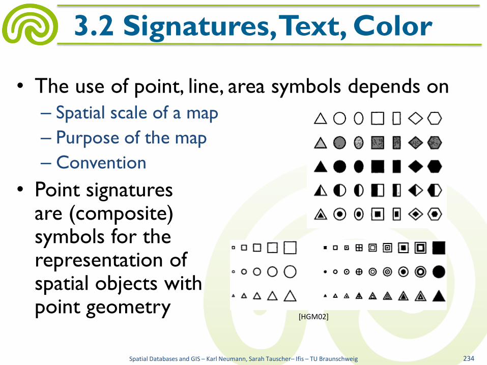
• The use of point, line, area symbols depends on
– Spatial scale of a map
– Purpose of the map
– Convention
• Point signatures are (composite) symbols for the representation of spatial objects with point geometry
Spatial Databases and GIS – Karl Neumann, Sarah Tauscher– Ifis – TU Braunschweig 234
3.2 Signatures, Text, Color
[HGM02]

• Line signatures represent objects with line geometry
• Area signatures represent objects with area geometry
• Texts are needed in various fonts for the labeling of maps
Spatial Databases and GIS – Karl Neumann, Sarah Tauscher– Ifis – TU Braunschweig 235
3.2 Signatures, Text, Color
[HGM02]

• Color
– Important design element
– Additive mixture
• Most relevant for displaying maps
on screen
• Common color space: RGB
– Subtractive mixture
• Most relevant for printing maps
• Common color space: CMYK
Spatial Databases and GIS – Karl Neumann, Sarah Tauscher– Ifis – TU Braunschweig 236
3.2 Signatures, Text, Color
htt
p:/
/ww
w.h
orr
ors
eek.
com
/ h
ttp
://a
cad
emic
.scr
anto
n.e
du
/
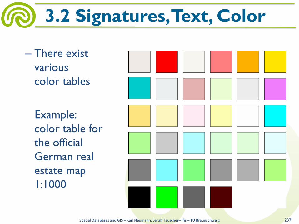
– There exist
various
color tables
Example:
color table for
the official
German real
estate map
1:1000
Spatial Databases and GIS – Karl Neumann, Sarah Tauscher– Ifis – TU Braunschweig 237
3.2 Signatures, Text, Color
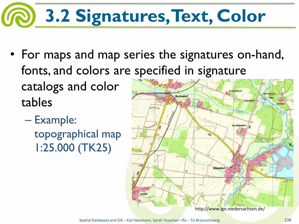
• For maps and map series the signatures on-hand,
fonts, and colors are specified in signature
catalogs and color
tables
– Example:
topographical map
1:25.000 (TK25)
Spatial Databases and GIS – Karl Neumann, Sarah Tauscher– Ifis – TU Braunschweig 238
3.2 Signatures, Text, Color
http://www.lgn.niedersachsen.de/

• Signature catalog "SK25" describes how the TK25 is derived
from the "digital landscape model" (digitales
Landschaftsmodell 1:25.000, DLM25)
• The catalog consists of derivation rules and signatures
(about
300
forms)
• Some
derivation
rules:
Spatial Databases and GIS – Karl Neumann, Sarah Tauscher– Ifis – TU Braunschweig 239
3.2 Signatures, Text, Color

• Some signatures:
Spatial Databases and GIS – Karl Neumann, Sarah Tauscher– Ifis – TU Braunschweig 240
3.2 Signatures, Text, Color

– Example:
real estate map 1:1000
• The ALKIS project (official property cadastre information
system, Amtliches Liegenschaftskataster Informationssystem)
specifies a signature library and derivation rules
• Approximately 670 signatures
• Approximately 850 derivation rules
Spatial Databases and GIS – Karl Neumann, Sarah Tauscher– Ifis – TU Braunschweig 241
3.2 Signatures, Text, Color
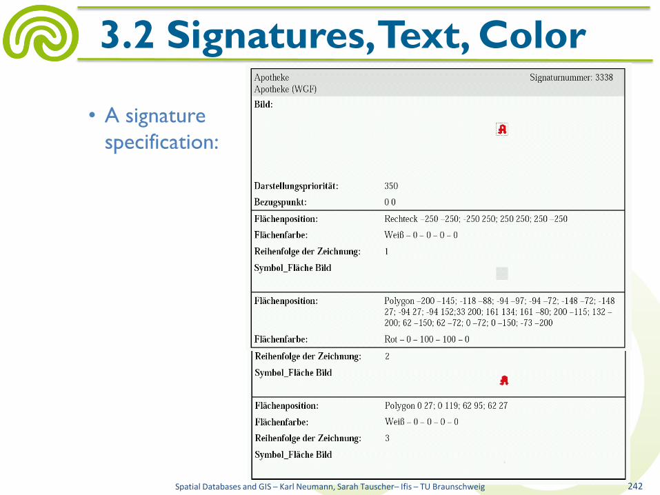
• A signature
specification:
Spatial Databases and GIS – Karl Neumann, Sarah Tauscher– Ifis – TU Braunschweig 242
3.2 Signatures, Text, Color
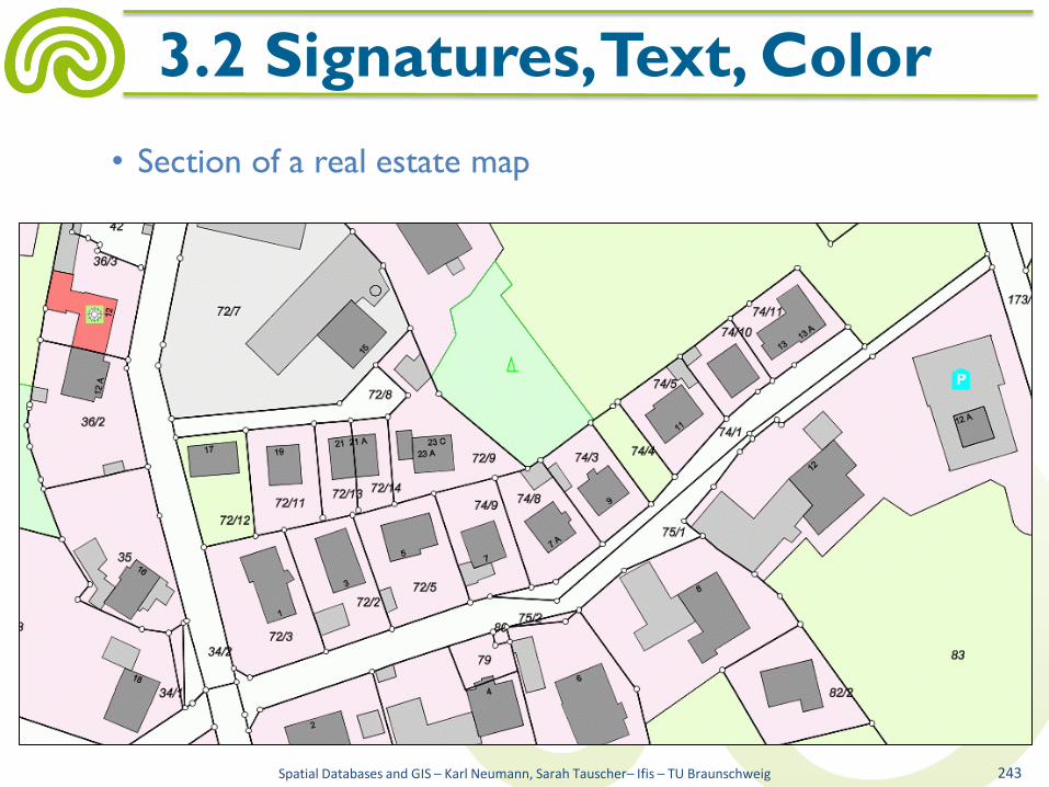
• Section of a real estate map
Spatial Databases and GIS – Karl Neumann, Sarah Tauscher– Ifis – TU Braunschweig 243
3.2 Signatures, Text, Color
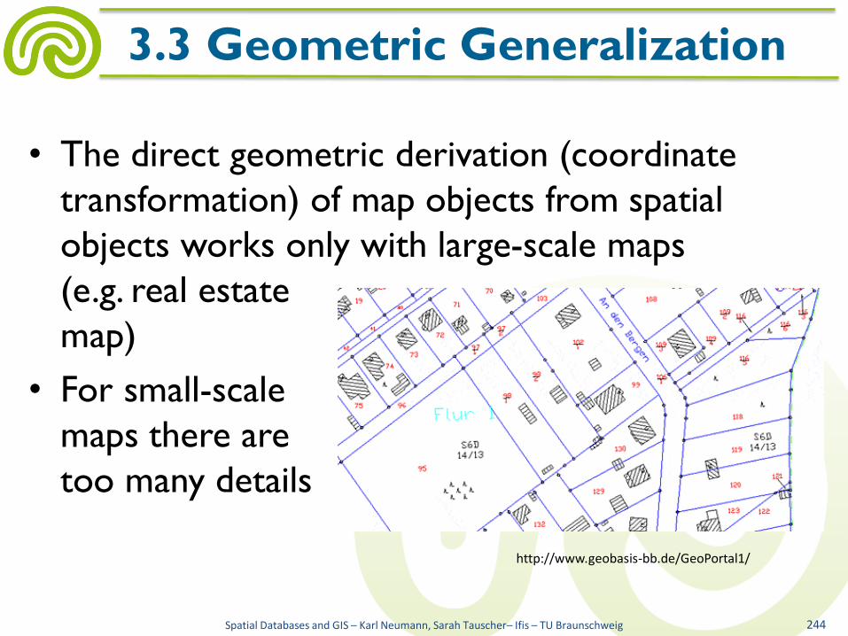
• The direct geometric derivation (coordinate
transformation) of map objects from spatial
objects works only with large-scale maps
(e.g. real estate
map)
• For small-scale
maps there are
too many details
Spatial Databases and GIS – Karl Neumann, Sarah Tauscher– Ifis – TU Braunschweig 244
3.3 Geometric Generalization
http://www.geobasis-bb.de/GeoPortal1/

• Generalization simplifies map content for the
preservation of readability and comprehensibility
• Replacement of scale preserving mappings
through simplified mappings, symbols, and
signatures
• Select and summarize information
• Maintain important objects, leave
out unimportant ones
Spatial Databases and GIS – Karl Neumann, Sarah Tauscher– Ifis – TU Braunschweig 245
3.3 Geometric Generalization
http://www.kartographie.info/

• Eight elementary operations
– To simplify
– To enlarge
– To displace
– To merge
Spatial Databases and GIS – Karl Neumann, Sarah Tauscher– Ifis – TU Braunschweig 246
3.3 Geometric Generalization
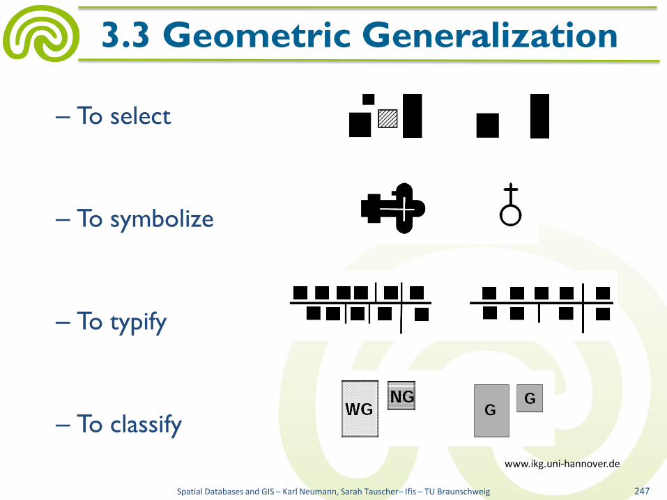
– To select
– To symbolize
– To typify
– To classify
Spatial Databases and GIS – Karl Neumann, Sarah Tauscher– Ifis – TU Braunschweig 247
3.3 Geometric Generalization
www.ikg.uni-hannover.de

Spatial Databases and GIS – Karl Neumann, Sarah Tauscher– Ifis – TU Braunschweig 248
3.3 Geometric Generalization
Base map 1:5000 Topographical map 1:25.000
[HGM02] [HGM02]

Spatial Databases and GIS – Karl Neumann, Sarah Tauscher– Ifis – TU Braunschweig 249
3.3 Geometric Generalization
Topographical map 1:25.000 Topographical map 1:50.000
[HGM02] [HGM02]
Spatial Databases and GIS – Karl Neumann, Sarah Tauscher– Ifis – TU Braunschweig 250
3.3 Geometric Generalization
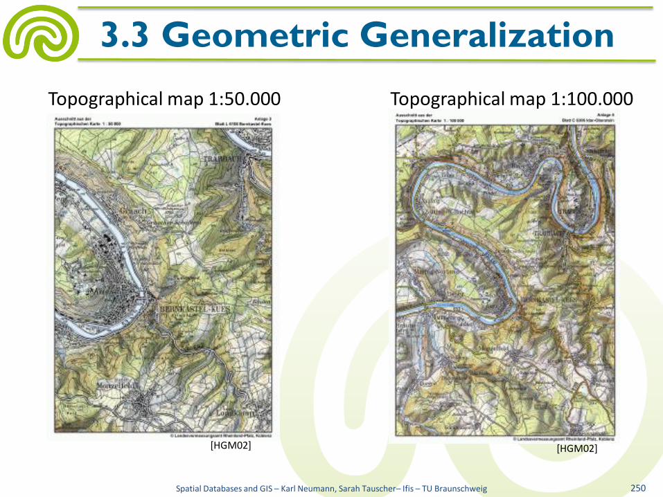
Topographical map 1:50.000 Topographical map 1:100.000
[HGM02] [HGM02]

• Typical operations for generalization
(alternative view)
Spatial Databases and GIS – Karl Neumann, Sarah Tauscher– Ifis – TU Braunschweig 251
3.3 Geometric Generalization
[SX08]

• Smoothing of polylines by means of a simple
low-pass filter:
y(n) = 1/3(x(n)+x(n−1)+x(n−2))
Spatial Databases and GIS – Karl Neumann, Sarah Tauscher– Ifis – TU Braunschweig 252
3.3 Geometric Generalization
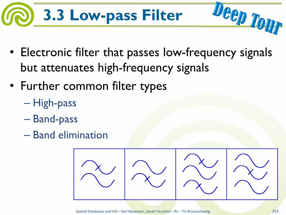
• Electronic filter that passes low-frequency signals
but attenuates high-frequency signals
• Further common filter types
– High-pass
– Band-pass
– Band elimination
Spatial Databases and GIS – Karl Neumann, Sarah Tauscher– Ifis – TU Braunschweig 253
3.3 Low-pass Filter
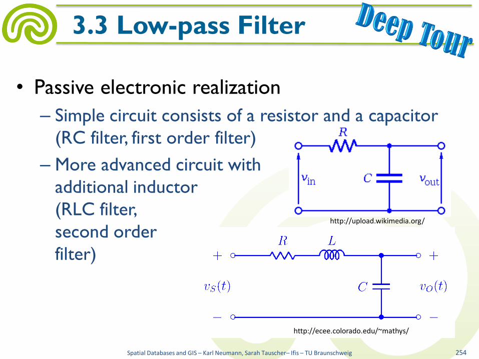
• Passive electronic realization
– Simple circuit consists of a resistor and a capacitor
(RC filter, first order filter)
– More advanced circuit with
additional inductor
(RLC filter,
second order
filter)
Spatial Databases and GIS – Karl Neumann, Sarah Tauscher– Ifis – TU Braunschweig 254
3.3 Low-pass Filter
http://upload.wikimedia.org/
http://ecee.colorado.edu/~mathys/

• Active electronic realization
– For example RC filter with an operational amplifier
– An operational amplifier has a high input impedance
and a low output
impedance
– Voltage gain is
determined by
resistors R1, R2
Spatial Databases and GIS – Karl Neumann, Sarah Tauscher– Ifis – TU Braunschweig 255
3.3 Low-pass Filter
http://www.electronics-tutorials.ws/

• Digital filters are realized as
– Finite impulse response
filter (FIR)
• Impulse response lasts for
n+1 samples and settles to zero
• Output is a weighted sum of
the current and a finite
number of previous values
of the input
– Infinite impulse response
filter (IIR)
Spatial Databases and GIS – Karl Neumann, Sarah Tauscher– Ifis – TU Braunschweig 256
3.3 Low-pass Filter
http://upload.wikimedia.org/
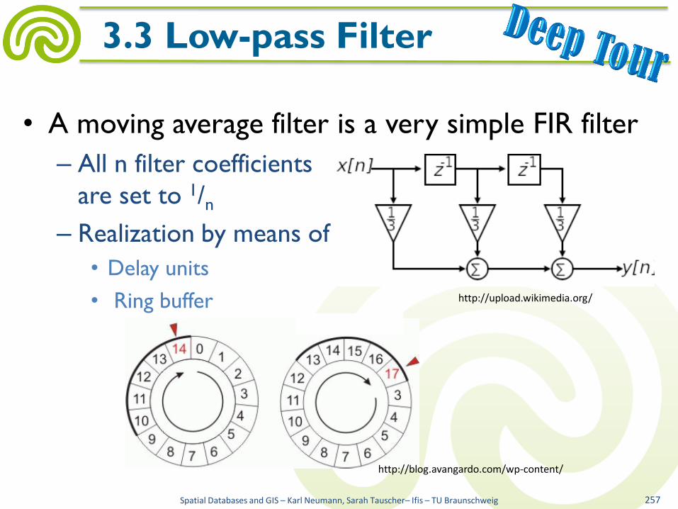
• A moving average filter is a very simple FIR filter
– All n filter coefficients
are set to 1/n
– Realization by means of
• Delay units
• Ring buffer
Spatial Databases and GIS – Karl Neumann, Sarah Tauscher– Ifis – TU Braunschweig 257
3.3 Low-pass Filter
http://upload.wikimedia.org/
http://blog.avangardo.com/wp-content/

• In offline mode (no real-time constraints)
a moving average filter results in a simple loop
Spatial Databases and GIS – Karl Neumann, Sarah Tauscher– Ifis – TU Braunschweig 258
3.3 Low-pass Filter
x[1...n] input values y[1...n] output values for (int i=2; i<n; i++) { y[i] = 0.333*(x[i-1]+x[i]+x[i+1]); }; y[1] = x[1]; y[n] = x[n];

• Adaptation of simple low-pass filter to
two-dimensional
geometry
x′i = ⅓(xi−1 +xi+ xi+1)
y′i = ⅓(yi−1 +yi + yi+1)
+ very efficiently to compute
− coordinates are changed, no reduction of points
Spatial Databases and GIS – Karl Neumann, Sarah Tauscher– Ifis – TU Braunschweig 259
3.3 Geometric Generalization

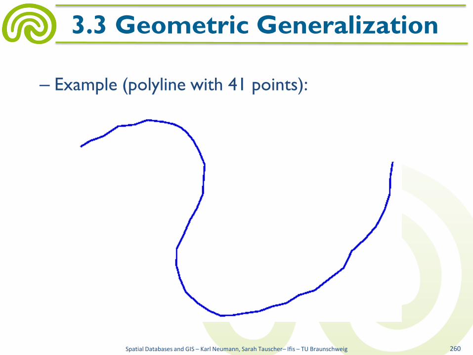
– Example (polyline with 41 points):
Spatial Databases and GIS – Karl Neumann, Sarah Tauscher– Ifis – TU Braunschweig 260
3.3 Geometric Generalization
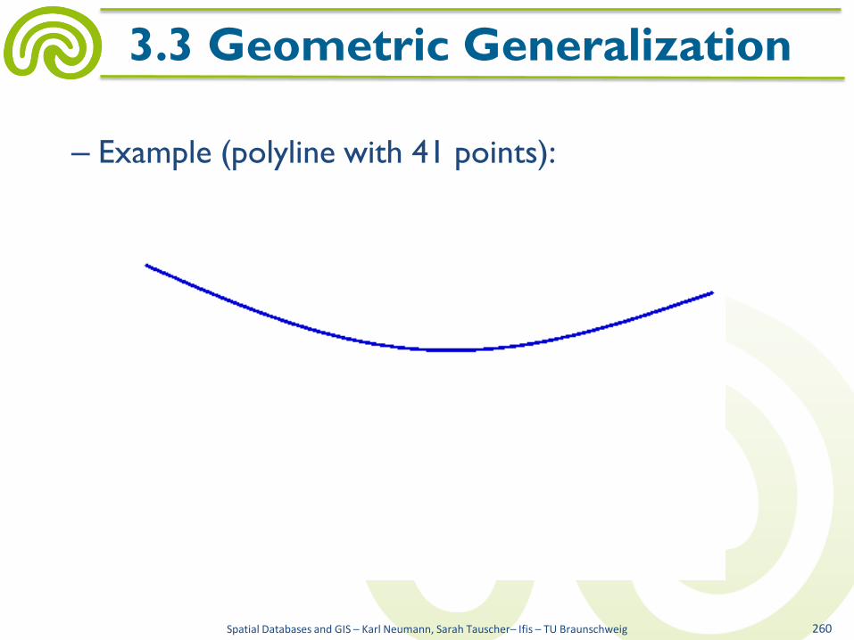
– Example (polyline with 41 points):
Spatial Databases and GIS – Karl Neumann, Sarah Tauscher– Ifis – TU Braunschweig 260
3.3 Geometric Generalization

– Example (polyline with 41 points):
Spatial Databases and GIS – Karl Neumann, Sarah Tauscher– Ifis – TU Braunschweig 260
3.3 Geometric Generalization
– Example (polyline with 41 points):
Spatial Databases and GIS – Karl Neumann, Sarah Tauscher– Ifis – TU Braunschweig 260
3.3 Geometric Generalization

– Example (polyline with 41 points):
Spatial Databases and GIS – Karl Neumann, Sarah Tauscher– Ifis – TU Braunschweig 260
3.3 Geometric Generalization
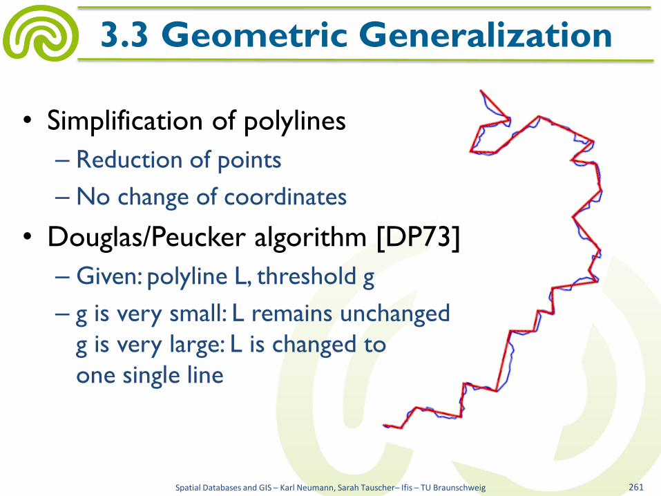
• Simplification of polylines
– Reduction of points
– No change of coordinates
• Douglas/Peucker algorithm [DP73]
– Given: polyline L, threshold g
– g is very small: L remains unchanged
g is very large: L is changed to
one single line
Spatial Databases and GIS – Karl Neumann, Sarah Tauscher– Ifis – TU Braunschweig 261
3.3 Geometric Generalization
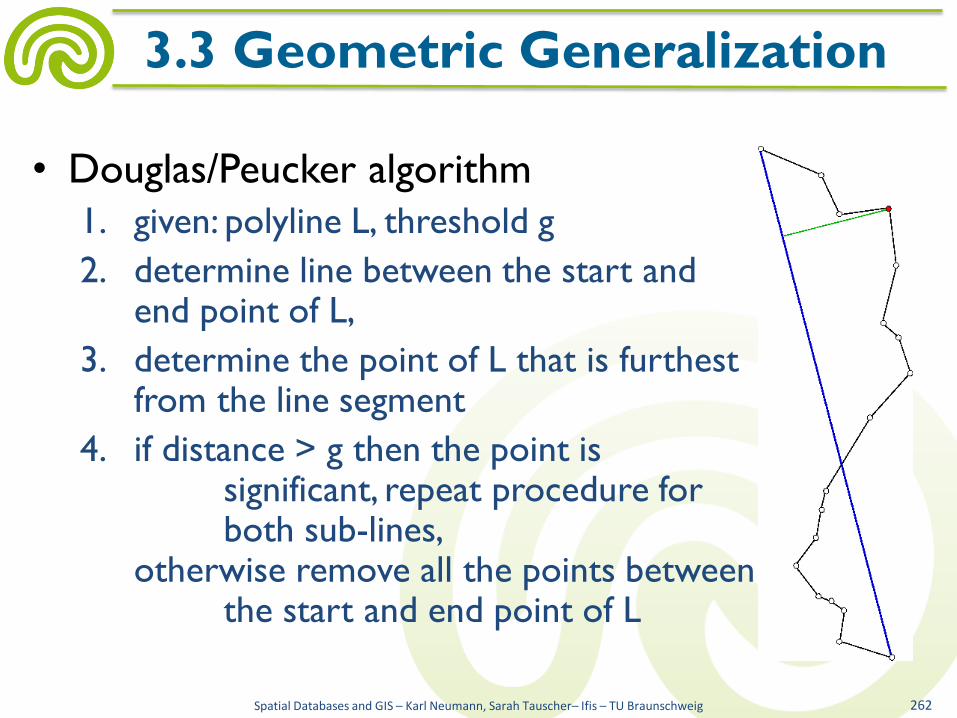
• Douglas/Peucker algorithm
1. given: polyline L, threshold g
2. determine line between the start and end point of L,
3. determine the point of L that is furthest from the line segment
4. if distance > g then the point is significant, repeat procedure for both sub-lines, otherwise remove all the points between the start and end point of L
Spatial Databases and GIS – Karl Neumann, Sarah Tauscher– Ifis – TU Braunschweig 262
3.3 Geometric Generalization

Examples:
Spatial Databases and GIS – Karl Neumann, Sarah Tauscher– Ifis – TU Braunschweig 263
3.3 Geometric Generalization

Spatial Databases and GIS – Karl Neumann, Sarah Tauscher– Ifis – TU Braunschweig 264
3.3 Geometric Generalization
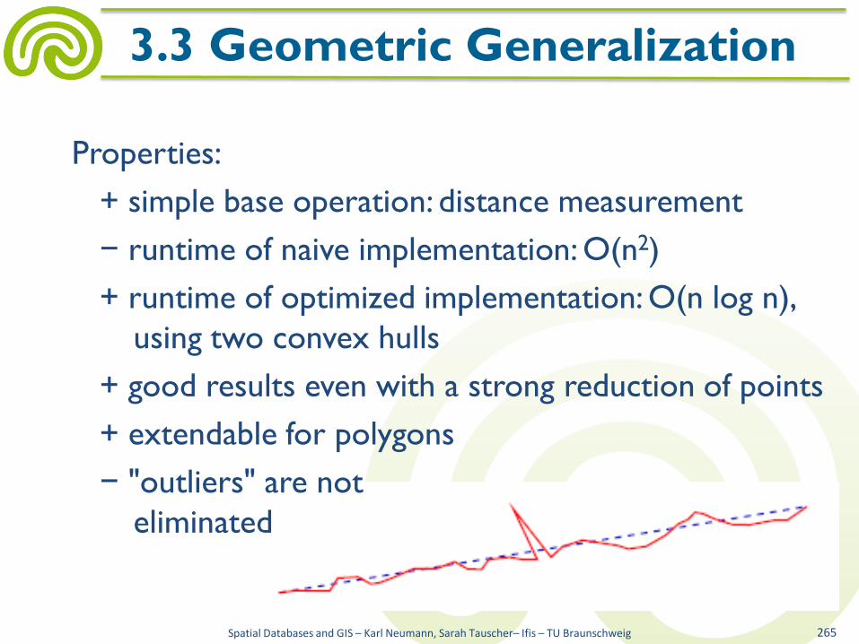
Properties:
+ simple base operation: distance measurement
− runtime of naive implementation: O(n2)
+ runtime of optimized implementation: O(n log n),
using two convex hulls
+ good results even with a strong reduction of points
+ extendable for polygons
− "outliers" are not
eliminated
Spatial Databases and GIS – Karl Neumann, Sarah Tauscher– Ifis – TU Braunschweig 265
3.3 Geometric Generalization

• Polygon to polyline conversion
– Presentation of rivers and roads
– Text placement within polygons
Spatial Databases and GIS – Karl Neumann, Sarah Tauscher– Ifis – TU Braunschweig 266
3.3 Geometric Generalization
http://www.almenrausch.at/bergtouren/ http://www.naturathlon2006.de/
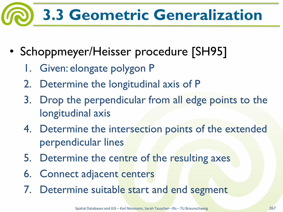
• Schoppmeyer/Heisser procedure [SH95]
1. Given: elongate polygon P
2. Determine the longitudinal axis of P
3. Drop the perpendicular from all edge points to the
longitudinal axis
4. Determine the intersection points of the extended
perpendicular lines
5. Determine the centre of the resulting axes
6. Connect adjacent centers
7. Determine suitable start and end segment
Spatial Databases and GIS – Karl Neumann, Sarah Tauscher– Ifis – TU Braunschweig 267
3.3 Geometric Generalization

Example
1. Given: elongate polygon P
2. Determine the longitudinal axis of P
Spatial Databases and GIS – Karl Neumann, Sarah Tauscher– Ifis – TU Braunschweig 268
3.3 Geometric Generalization

3. Drop the perpendicular from all edge points to the
longitudinal axis
4. Determine the intersection points of the extended
perpendicular lines
Spatial Databases and GIS – Karl Neumann, Sarah Tauscher– Ifis – TU Braunschweig 269
3.3 Geometric Generalization

5. Determine the centre of the resulting axes
6. Connect adjacent centers
Spatial Databases and GIS – Karl Neumann, Sarah Tauscher– Ifis – TU Braunschweig 270
3.3 Geometric Generalization
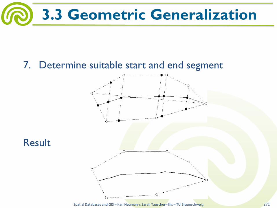
7. Determine suitable start and end segment
Result
Spatial Databases and GIS – Karl Neumann, Sarah Tauscher– Ifis – TU Braunschweig 271
3.3 Geometric Generalization

Using the result for text placement
Spatial Databases and GIS – Karl Neumann, Sarah Tauscher– Ifis – TU Braunschweig 272
3.3 Geometric Generalization

Properties:
+ relatively short runtime
+ quite good results with "good-natured" polygons
− determining the start and end segment
− procedure fails for
non-elongate
polygons
Spatial Databases and GIS – Karl Neumann, Sarah Tauscher– Ifis – TU Braunschweig 273
3.3 Geometric Generalization
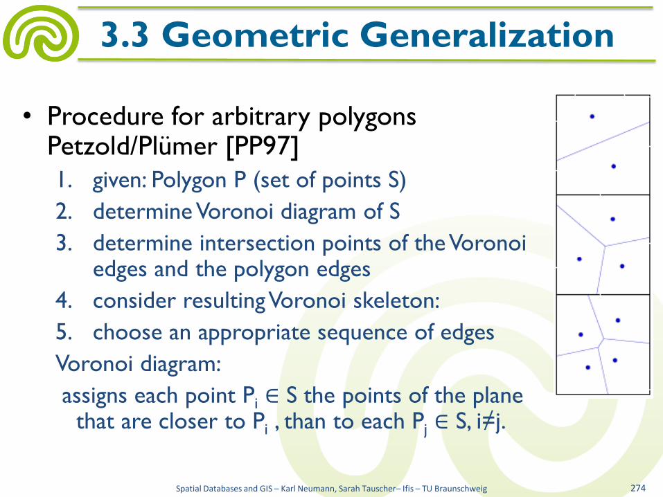
• Procedure for arbitrary polygons Petzold/Plümer [PP97]
1. given: Polygon P (set of points S)
2. determine Voronoi diagram of S
3. determine intersection points of the Voronoi edges and the polygon edges
4. consider resulting Voronoi skeleton:
5. choose an appropriate sequence of edges
Voronoi diagram:
assigns each point Pi ∈ S the points of the plane that are closer to Pi , than to each Pj ∈ S, i≠j.
Spatial Databases and GIS – Karl Neumann, Sarah Tauscher– Ifis – TU Braunschweig 274
3.3 Geometric Generalization
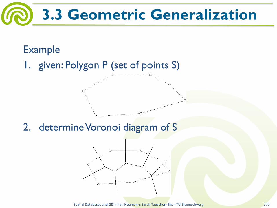
Example
1. given: Polygon P (set of points S)
2. determine Voronoi diagram of S
Spatial Databases and GIS – Karl Neumann, Sarah Tauscher– Ifis – TU Braunschweig 275
3.3 Geometric Generalization

3. determine intersection points of the Voronoi edges
and the polygon edges
4. consider resulting Voronoi skeleton:
5. choose an appropriate sequence of edges
Spatial Databases and GIS – Karl Neumann, Sarah Tauscher– Ifis – TU Braunschweig 276
3.3 Geometric Generalization
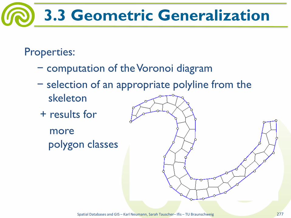
Properties:
− computation of the Voronoi diagram
− selection of an appropriate polyline from the
skeleton
+ results for
more
polygon classes
Spatial Databases and GIS – Karl Neumann, Sarah Tauscher– Ifis – TU Braunschweig 277
3.3 Geometric Generalization

Example (polygon with 2000 points):
Spatial Databases and GIS – Karl Neumann, Sarah Tauscher– Ifis – TU Braunschweig 278
3.3 Geometric Generalization
visualization tool: [Me11]
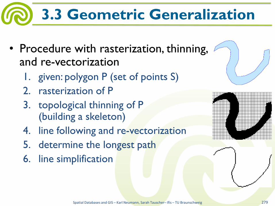
• Procedure with rasterization, thinning, and re-vectorization
1. given: polygon P (set of points S)
2. rasterization of P
3. topological thinning of P (building a skeleton)
4. line following and re-vectorization
5. determine the longest path
6. line simplification
Spatial Databases and GIS – Karl Neumann, Sarah Tauscher– Ifis – TU Braunschweig 279
3.3 Geometric Generalization

Example
1. given: polygon P (set of points S)
Spatial Databases and GIS – Karl Neumann, Sarah Tauscher– Ifis – TU Braunschweig 280
3.3 Geometric Generalization
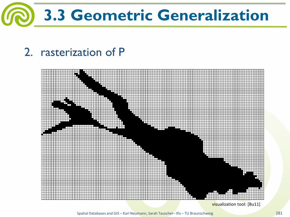
2. rasterization of P
Spatial Databases and GIS – Karl Neumann, Sarah Tauscher– Ifis – TU Braunschweig 281
3.3 Geometric Generalization
visualization tool: [Bu11]

3. topological thinning of P
Spatial Databases and GIS – Karl Neumann, Sarah Tauscher– Ifis – TU Braunschweig 282
3.3 Geometric Generalization
visualization tool: [Bu11]

4. line following and re-vectorization
Spatial Databases and GIS – Karl Neumann, Sarah Tauscher– Ifis – TU Braunschweig 283
3.3 Geometric Generalization
visualization tool: [Bu11]

5. determine the longest path
Spatial Databases and GIS – Karl Neumann, Sarah Tauscher– Ifis – TU Braunschweig 284
3.3 Geometric Generalization
visualization tool: [Bu11]

6. line simplification
Spatial Databases and GIS – Karl Neumann, Sarah Tauscher– Ifis – TU Braunschweig 285
3.3 Geometric Generalization
visualization tool: [Bu11]

• Simplification of polygons
– Low-pass filter
• Coordinates are changed
• No reduction of points
• Shapes might be drastically changed
Spatial Databases and GIS – Karl Neumann, Sarah Tauscher– Ifis – TU Braunschweig 286
3.3 Geometric Generalization

– Douglas/Peucker (adapted)
• Decompose polygon P into two polylines L1, L2 e.g. at the
points PL1, PL2 ∈ P, with maximum distance between each
other
• Simplify L1 and L2
• Recombine
resulting polylines
at PL1 and PL2
Spatial Databases and GIS – Karl Neumann, Sarah Tauscher– Ifis – TU Braunschweig 287
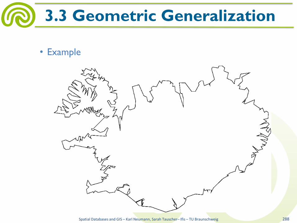
3.3 Geometric Generalization

• Example
Spatial Databases and GIS – Karl Neumann, Sarah Tauscher– Ifis – TU Braunschweig 288
3.3 Geometric Generalization

• Example
Spatial Databases and GIS – Karl Neumann, Sarah Tauscher– Ifis – TU Braunschweig 288
3.3 Geometric Generalization
• Example
Spatial Databases and GIS – Karl Neumann, Sarah Tauscher– Ifis – TU Braunschweig 288
3.3 Geometric Generalization
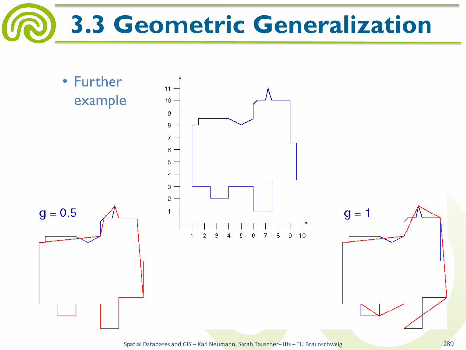
• Further
example
Spatial Databases and GIS – Karl Neumann, Sarah Tauscher– Ifis – TU Braunschweig 289
3.3 Geometric Generalization

Spatial Databases and GIS – Karl Neumann, Sarah Tauscher– Ifis – TU Braunschweig 290
3.3 Geometric Generalization
• Cartographically
desired
generalization
• Results with
Douglas/Peucker
(adapted)

• Douglas/Peucker reduces the number of polygon points
• Characteristic shapes are preserved (within certain limits)
• Good results with "natural" geometries (bogs, lakes, forests)
• Less satisfactory results with polygons with predominantly
right angles (buildings), therefore modification to preserve
right angles and long edges (e.g. [NSe01])
Spatial Databases and GIS – Karl Neumann, Sarah Tauscher– Ifis – TU Braunschweig 291
3.3 Geometric Generalization

• Geometric generalization (and displacement) of
building sketches is a challenging task
• Convenient results achieved by programs
• E.g. CHANGE, PUSH, TYPIFY [Se07]
Spatial Databases and GIS – Karl Neumann, Sarah Tauscher– Ifis – TU Braunschweig 292
3.3 Geometric Generalization
http://www.ikg.uni-hannover.de/

• Placement of all texts (labels) in the same way
results with high probability in overlappings (poor
readability)
• Therefore, it is necessary
to move, scale down,
rotate, or omit texts
• In the general case this is
a NP-hard optimization
problem
Spatial Databases and GIS – Karl Neumann, Sarah Tauscher– Ifis – TU Braunschweig 293
3.4 Label and Symbol Placement
http://www.laum.uni-hannover.de/ilr/lehre/Isv/

• Objectives of labeling
– Easily readable
– Unambiguity: each label must be easily identified with exactly one graphical feature
– Same facts are represented in the same way
– Different facts are represented differently
– Important facts are emphasized
– Important objects are never covered
– No uniform pattern (avoidance of raster effect)
Spatial Databases and GIS – Karl Neumann, Sarah Tauscher– Ifis – TU Braunschweig 294
3.4 Label and Symbol Placement
http://www.mdc.tu-dresden.de/

• Text or label placement is divided into
– Point labeling
• Positions to the right are preferred to those on the left
• Labels above a point are preferred to those below
• E.g. cities with a horizontal label
– Line labeling
• Labels should be placed as straight as possible
• E.g. rivers with names
– Area labeling
• It must be clear what the total area is
• E.g. forest areas containing their names
Spatial Databases and GIS – Karl Neumann, Sarah Tauscher– Ifis – TU Braunschweig 295
3.4 Label and Symbol Placement
http://www.sprachkurs-sprachschule.com/
http://upload.wikimedia.org/

• For the three classes there are many specialized
algorithms, based on
– Greedy algorithm
• Labels are placed in sequence
• Each position is chosen
according to minimal
overlapping
• Acceptable results only for
very simple problems
• Very fast
Spatial Databases and GIS – Karl Neumann, Sarah Tauscher– Ifis – TU Braunschweig 296
3.4 Label and Symbol Placement

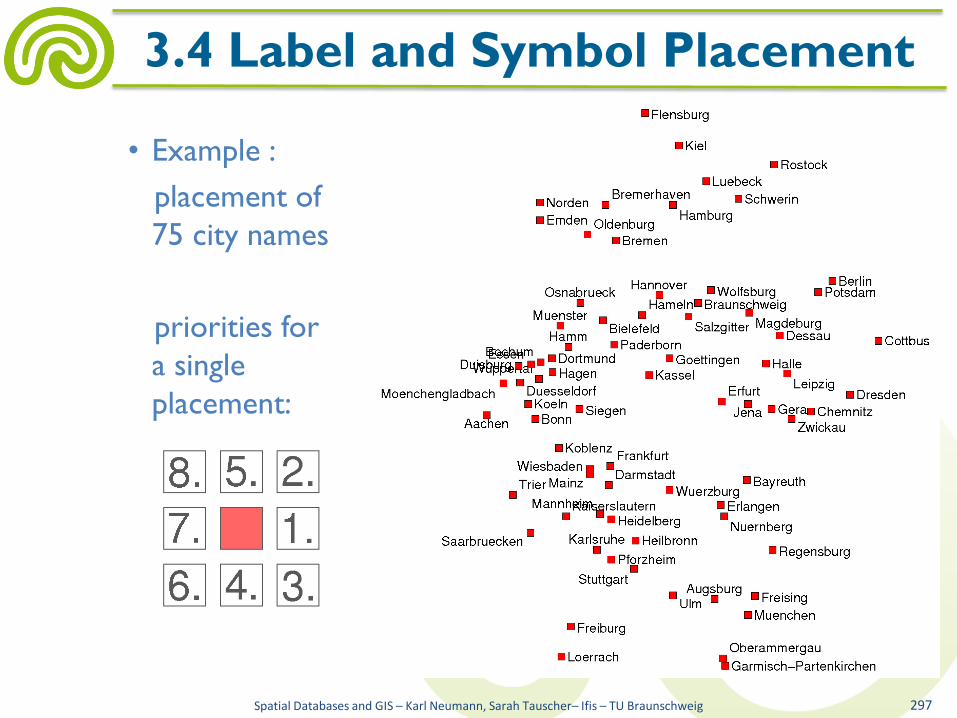
• Example :
placement of
75 city names
priorities for
a single
placement:
Spatial Databases and GIS – Karl Neumann, Sarah Tauscher– Ifis – TU Braunschweig 297
3.4 Label and Symbol Placement

• Example :
placement of
75 city names
priorities for
a single
placement:
Spatial Databases and GIS – Karl Neumann, Sarah Tauscher– Ifis – TU Braunschweig 297
3.4 Label and Symbol Placement

• Example :
placement of
75 city names
priorities for
a single
placement:
Spatial Databases and GIS – Karl Neumann, Sarah Tauscher– Ifis – TU Braunschweig 297
3.4 Label and Symbol Placement

• Example :
placement of
75 city names
priorities for
a single
placement:
Spatial Databases and GIS – Karl Neumann, Sarah Tauscher– Ifis – TU Braunschweig 297
3.4 Label and Symbol Placement

• Example :
placement of
75 city names
priorities for
a single
placement:
Spatial Databases and GIS – Karl Neumann, Sarah Tauscher– Ifis – TU Braunschweig 297
3.4 Label and Symbol Placement
• Example :
placement of
75 city names
priorities for
a single
placement:
Spatial Databases and GIS – Karl Neumann, Sarah Tauscher– Ifis – TU Braunschweig 297
3.4 Label and Symbol Placement
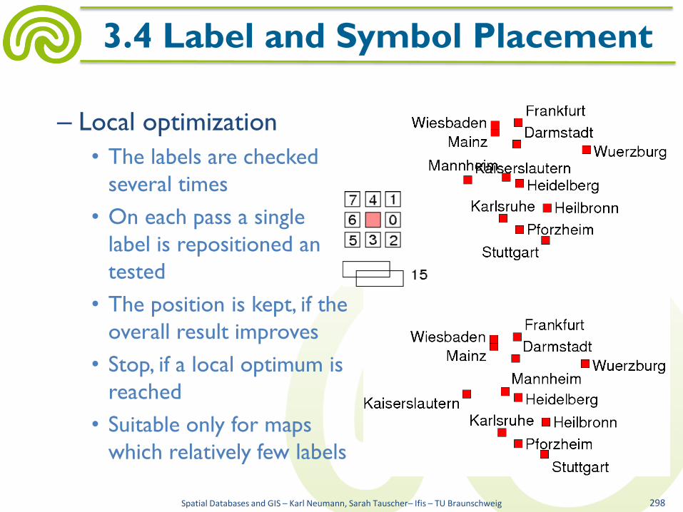
– Local optimization
• The labels are checked
several times
• On each pass a single
label is repositioned an
tested
• The position is kept, if the
overall result improves
• Stop, if a local optimum is
reached
• Suitable only for maps
which relatively few labels
Spatial Databases and GIS – Karl Neumann, Sarah Tauscher– Ifis – TU Braunschweig 298
3.4 Label and Symbol Placement
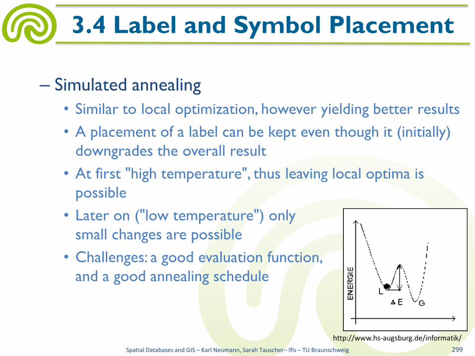
– Simulated annealing
• Similar to local optimization, however yielding better results
• A placement of a label can be kept even though it (initially)
downgrades the overall result
• At first "high temperature", thus leaving local optima is
possible
• Later on ("low temperature") only
small changes are possible
• Challenges: a good evaluation function,
and a good annealing schedule
Spatial Databases and GIS – Karl Neumann, Sarah Tauscher– Ifis – TU Braunschweig 299
3.4 Label and Symbol Placement
http://www.hs-augsburg.de/informatik/
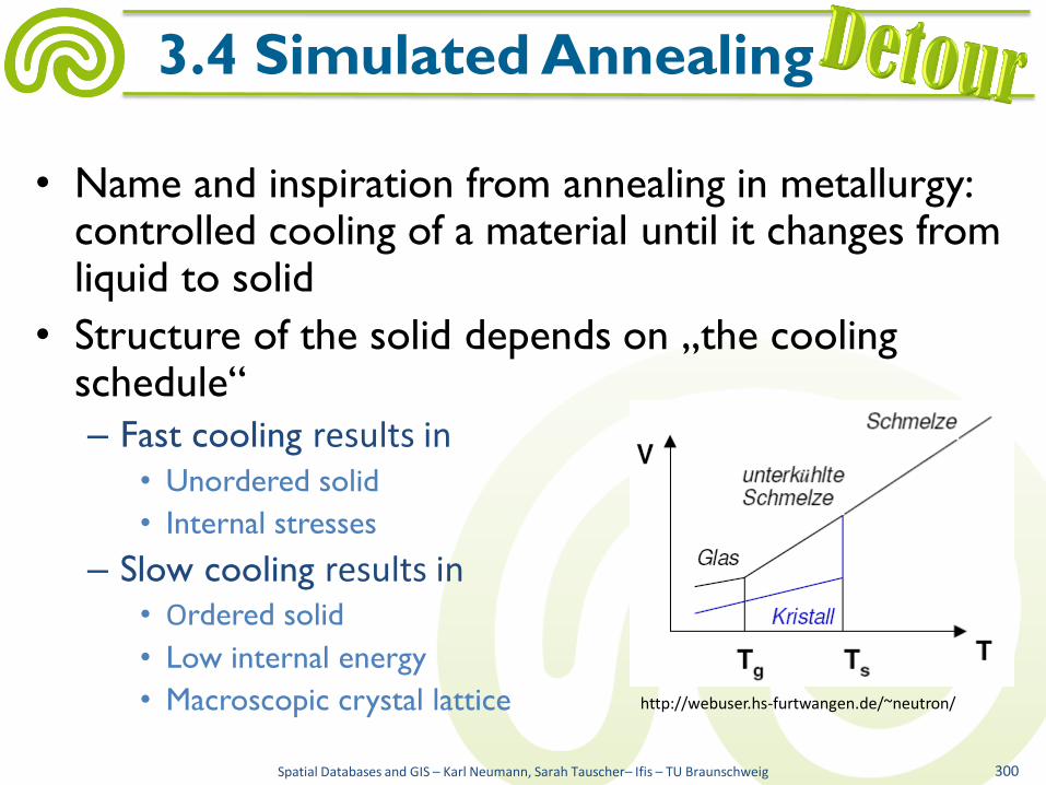
• Name and inspiration from annealing in metallurgy: controlled cooling of a material until it changes from liquid to solid
• Structure of the solid depends on „the cooling schedule“
– Fast cooling results in • Unordered solid
• Internal stresses
– Slow cooling results in • Ordered solid
• Low internal energy
• Macroscopic crystal lattice
Spatial Databases and GIS – Karl Neumann, Sarah Tauscher– Ifis – TU Braunschweig 300
3.4 Simulated Annealing
http://webuser.hs-furtwangen.de/~neutron/

• Example: SiO2
– Short range order: tetrahedron
– Crystalline form: Cristobalit
– Without long range order: Silica glass
Spatial Databases and GIS – Karl Neumann, Sarah Tauscher– Ifis – TU Braunschweig 301
3.4 Simulated Annealing
http://de.wikipedia.org/wiki/Glas
Si O
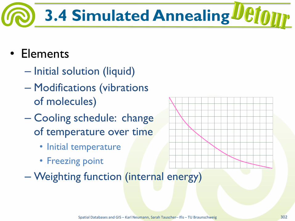
• Elements
– Initial solution (liquid)
– Modifications (vibrations
of molecules)
– Cooling schedule: change
of temperature over time
• Initial temperature
• Freezing point
– Weighting function (internal energy)
Spatial Databases and GIS – Karl Neumann, Sarah Tauscher– Ifis – TU Braunschweig 302
3.4 Simulated Annealing
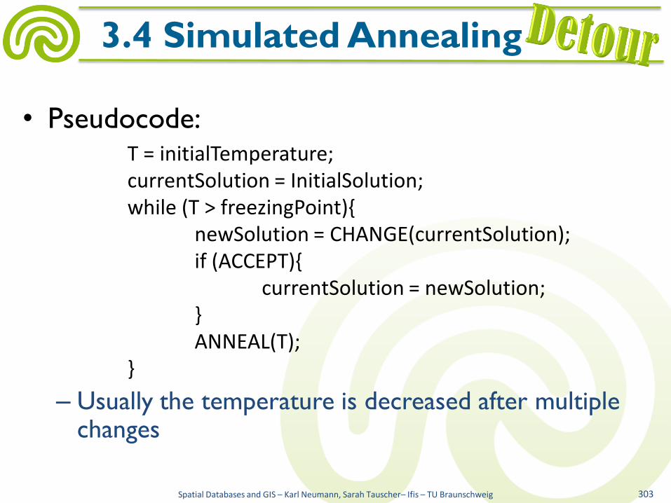
• Pseudocode:
– Usually the temperature is decreased after multiple changes
Spatial Databases and GIS – Karl Neumann, Sarah Tauscher– Ifis – TU Braunschweig 303
3.4 Simulated Annealing
T = initialTemperature; currentSolution = InitialSolution; while (T > freezingPoint){ newSolution = CHANGE(currentSolution); if (ACCEPT){ currentSolution = newSolution; } ANNEAL(T); }

– Decision if the new solution is accepted
• A better solution is always accepted
• Probability of accepting a worse solution depends on the
temperature and its cost
• Boltzmann factor: e-E/k*T ; k = 1,3806504(24) · 10−23
Spatial Databases and GIS – Karl Neumann, Sarah Tauscher– Ifis – TU Braunschweig 304
3.4 Simulated Annealing
ACCEPT{ Δ = EVALUATE(newSolution) – EVALUATE(currentSolution) if((Δ < 0) or RANDOM(0,1) < e-Δ/T)){ return true; } return false; }

• Example: label placement
Spatial Databases and GIS – Karl Neumann, Sarah Tauscher– Ifis – TU Braunschweig 305
3.4 Simulated Annealing
http://citeseerx.ist.psu.edu/viewdoc/summary?doi=10.1.1.50.2327

• Initial solution: random label placement
• Weighting function
– Number of covered (or deleted) labels
– Consideration of cartographic preferences by
weighting of possible positions for point labels
• Modifications
– Move an arbitrary or covered label to a new position
– If cartographic preferences are considered an
arbitrary label should be moved
Spatial Databases and GIS – Karl Neumann, Sarah Tauscher– Ifis – TU Braunschweig 306
3.4 Simulated Annealing
2 4 1
5
6
8
7 3

• Cooling schedule:
– Initial temperature ca 2,47 → the probability of accepting that a solution whose cost are 1 higher is accepted is 2/3, i.e.: e-1/T = 2/3
– T = 0,1 * T
– T is decreased as soon as more than 5*n new solutions have been accepted (n is the number of objects)
– Search ends
• As soon as T has been decreased 50 times
• If none of 20*n new solutions in a row has been accepted
Spatial Databases and GIS – Karl Neumann, Sarah Tauscher– Ifis – TU Braunschweig 307
3.4 Simulated Annealing
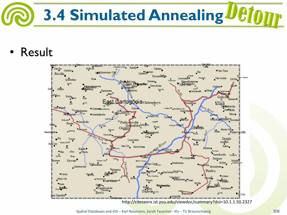
• Result
Spatial Databases and GIS – Karl Neumann, Sarah Tauscher– Ifis – TU Braunschweig 308
3.4 Simulated Annealing
http://citeseerx.ist.psu.edu/viewdoc/summary?doi=10.1.1.50.2327

• Result
Spatial Databases and GIS – Karl Neumann, Sarah Tauscher– Ifis – TU Braunschweig 308
3.4 Simulated Annealing
http://citeseerx.ist.psu.edu/viewdoc/summary?doi=10.1.1.50.2327
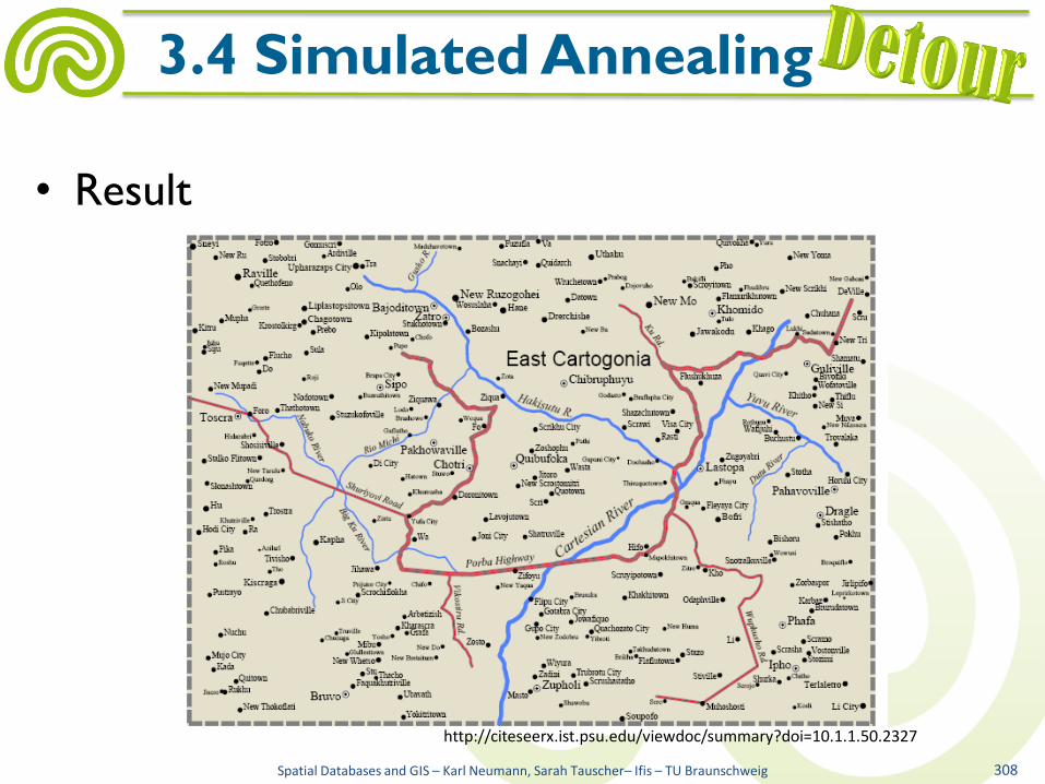
• Result
Spatial Databases and GIS – Karl Neumann, Sarah Tauscher– Ifis – TU Braunschweig 308
3.4 Simulated Annealing
http://citeseerx.ist.psu.edu/viewdoc/summary?doi=10.1.1.50.2327

• Symbol placement (point signatures) is just as
complex as text placement
• In the following two examples for special cases
– Displacement and placement
of tree symbols in TK25-like
presentation graphics
[NPW06]
– Placement of point signatures
in polygons of buildings for
real estate maps [NKP08]
Spatial Databases and GIS – Karl Neumann, Sarah Tauscher– Ifis – TU Braunschweig 309
3.4 Label and Symbol Placement
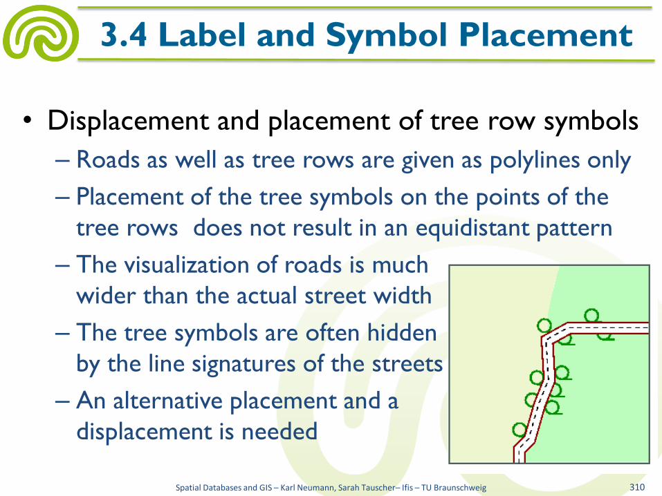
• Displacement and placement of tree row symbols
– Roads as well as tree rows are given as polylines only
– Placement of the tree symbols on the points of the
tree rows does not result in an equidistant pattern
– The visualization of roads is much
wider than the actual street width
– The tree symbols are often hidden
by the line signatures of the streets
– An alternative placement and a
displacement is needed
Spatial Databases and GIS – Karl Neumann, Sarah Tauscher– Ifis – TU Braunschweig 310
3.4 Label and Symbol Placement

• One single road from the DLM25
(example, XML/GML encoding)
Spatial Databases and GIS – Karl Neumann, Sarah Tauscher– Ifis – TU Braunschweig 311
3.4 Label and Symbol Placement
<AtkisMember> <Strasse> <gml:name> Badstrasse </gml:name> <AtkisOID> 86118065 </AtkisOID> <gml:centerLineOf> <gml:coord><gml:X>4437952.980</gml:X><gml:Y>5331812.550</gml:Y></gml:coord> <gml:coord><gml:X>4437960.070</gml:X><gml:Y>5331818.450</gml:Y></gml:coord> <gml:coord><gml:X>4437967.200</gml:X><gml:Y>5331825.410</gml:Y> </gml:coord> </gml:centerLineOf> <Attribute> <Zustand> in Betrieb </Zustand> <AnzahlDerFahrstreifen Bedeutung=“tatsaechliche Anzahl”> 2 </AnzahlDerFahrstreifen> <Funktion> Strassenverkehr </Funktion> <VerkehrsbedeutungInneroertlich> Anliegerverkehr </VerkehrsbedeutungInneroertlich> <Widmung> Gemeindestrasse </Widmung> </Attribute> </Strasse> </AtkisMember>
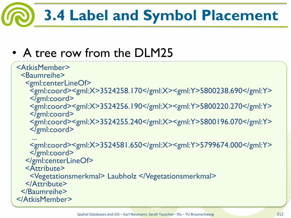
• A tree row from the DLM25
Spatial Databases and GIS – Karl Neumann, Sarah Tauscher– Ifis – TU Braunschweig 312
3.4 Label and Symbol Placement
<AtkisMember> <Baumreihe> <gml:centerLineOf> <gml:coord><gml:X>3524258.170</gml:X><gml:Y>5800238.690</gml:Y> </gml:coord> <gml:coord><gml:X>3524256.190</gml:X><gml:Y>5800220.270</gml:Y> </gml:coord> <gml:coord><gml:X>3524255.240</gml:X><gml:Y>5800196.070</gml:Y> </gml:coord> ... <gml:coord><gml:X>3524581.650</gml:X><gml:Y>5799674.000</gml:Y> </gml:coord> </gml:centerLineOf> <Attribute> <Vegetationsmerkmal> Laubholz </Vegetationsmerkmal> </Attribute> </Baumreihe> </AtkisMember>

• Direct visualization
Spatial Databases and GIS – Karl Neumann, Sarah Tauscher– Ifis – TU Braunschweig 313
3.4 Label and Symbol Placement

• Simple displacement procedure
Spatial Databases and GIS – Karl Neumann, Sarah Tauscher– Ifis – TU Braunschweig 314
3.4 Label and Symbol Placement
for all t : treeRow do begin if exists s : street (distance(t,s) ≤ minDistance(s.dedication)) then for all p : t.coord do begin r := refSegment(s,p); move(p,r) end do end if end do;

• Visualization with displacement
Spatial Databases and GIS – Karl Neumann, Sarah Tauscher– Ifis – TU Braunschweig 315
3.4 Label and Symbol Placement

• Placement procedure
Spatial Databases and GIS – Karl Neumann, Sarah Tauscher– Ifis – TU Braunschweig 316
3.4 Label and Symbol Placement
for all t : treeRow do begin l := length(t.centerLineOf); n := ⌊l/distanceConst⌋ + 1; t’ : new treeRow; for i=1 to n do begin computePoint (t’.coord[i], t.centerLineOf, distanceConst) end do end do;

• Visualization with displacement and placement
Spatial Databases and GIS – Karl Neumann, Sarah Tauscher– Ifis – TU Braunschweig 317
3.4 Label and Symbol Placement

• Placement of point signatures in polygons of buildings
– Derivation of the real estate map (1:1.000) from ALKIS inventory data extracts relatively straight forward
– No generalization and no displacement is needed
– Representation of buildings, parcels, border points, etc., with the given signature library and the derivation rules
– E.g. symbolisation of buildings as colored polygons with a boundary line and a typical point signature depending on the attribute building function
Spatial Databases and GIS – Karl Neumann, Sarah Tauscher– Ifis – TU Braunschweig 318
3.4 Label and Symbol Placement
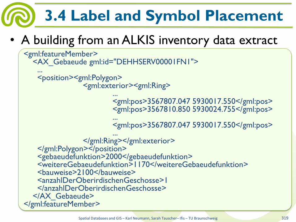
• A building from an ALKIS inventory data extract
Spatial Databases and GIS – Karl Neumann, Sarah Tauscher– Ifis – TU Braunschweig 319
3.4 Label and Symbol Placement
<gml:featureMember> <AX_Gebaeude gml:id="DEHHSERV00001FN1"> ... <position><gml:Polygon> <gml:exterior><gml:Ring> ... <gml:pos>3567807.047 5930017.550</gml:pos> <gml:pos>3567810.850 5930024.755</gml:pos> ... <gml:pos>3567807.047 5930017.550</gml:pos> ... </gml:Ring></gml:exterior> </gml:Polygon></position> <gebaeudefunktion>2000</gebaeudefunktion> <weitereGebaeudefunktion>1170</weitereGebaeudefunktion> <bauweise>2100</bauweise> <anzahlDerOberirdischenGeschosse>1 </anzahlDerOberirdischenGeschosse> </AX_Gebaeude> </gml:featureMember>
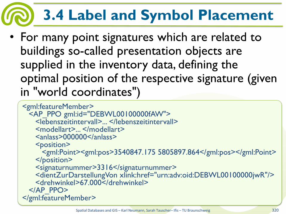
• For many point signatures which are related to buildings so-called presentation objects are supplied in the inventory data, defining the optimal position of the respective signature (given in "world coordinates")
Spatial Databases and GIS – Karl Neumann, Sarah Tauscher– Ifis – TU Braunschweig 320
3.4 Label and Symbol Placement
<gml:featureMember> <AP_PPO gml:id="DEBWL00100000fAW"> <lebenszeitintervall>... </lebenszeitintervall> <modellart>... </modellart> <anlass>000000</anlass> <position> <gml:Point><gml:pos>3540847.175 5805897.864</gml:pos></gml:Point> </position> <signaturnummer>3316</signaturnummer> <dientZurDarstellungVon xlink:href="urn:adv:oid:DEBWL00100000jwR"/> <drehwinkel>67.000</drehwinkel> </AP_PPO> </gml:featureMember>

• But some buildings lack the presentation objects
• An obvious, easily determined position for the
signature:
– Choose the center of the smallest axis parallel
rectangle, which encloses the polygon of the building
– min(x1, ..., xn)+((max(x1, ..., xn)−min(x1, ..., xn))/2),
– min(y1, ..., yn)+((max(y1, ..., yn)−min(y1, ..., yn))/2)
Spatial Databases and GIS – Karl Neumann, Sarah Tauscher– Ifis – TU Braunschweig 321
3.4 Label and Symbol Placement

• Unfortunately, the results are not always satisfactory
• Therefore, heuristic procedure, based on
– Convexity
– (approximate) symmetry points
– (approximate) symmetry axis
– Various quality criteria
– Discrete increments
Spatial Databases and GIS – Karl Neumann, Sarah Tauscher– Ifis – TU Braunschweig 322
3.4 Label and Symbol Placement

Spatial Databases and GIS – Karl Neumann, Sarah Tauscher– Ifis – TU Braunschweig 323
3.4 Label and Symbol Placement
if polygon of building convex: choose centroid if signature frame fits completely in polygon of building: place there otherwise choose appropriate point with the smallest distance to the centroid else if symmetry point in polygon of building: place there otherwise further procedure with symmetry axes
⇒ generation of a new presentation object with "optimal" positioning coordinates
centroid
best symmetry point
best symmetry axis
finally chosen point
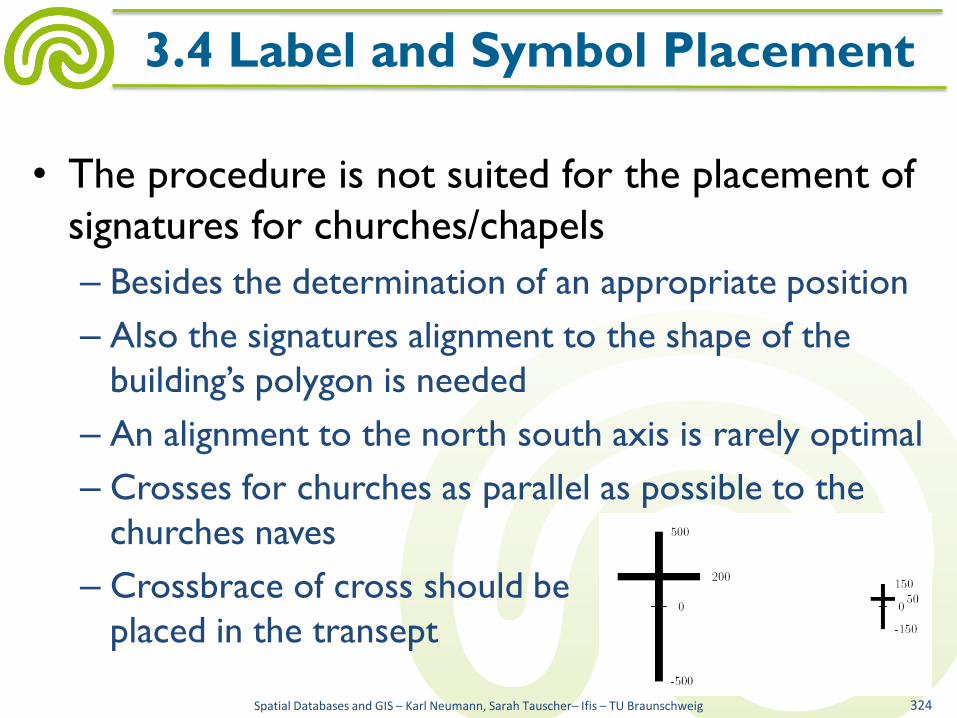
• The procedure is not suited for the placement of
signatures for churches/chapels
– Besides the determination of an appropriate position
– Also the signatures alignment to the shape of the
building’s polygon is needed
– An alignment to the north south axis is rarely optimal
– Crosses for churches as parallel as possible to the
churches naves
– Crossbrace of cross should be
placed in the transept
Spatial Databases and GIS – Karl Neumann, Sarah Tauscher– Ifis – TU Braunschweig 324
3.4 Label and Symbol Placement

• Heuristic procedure
– Determine a preferable large cross that just fits in the
building’s polygon
– Proportions of the large cross and the church
signature are the same
– If the large cross is found, place the signature just in
the intersection point
• For this purpose first simplify the building’s
polygon
Spatial Databases and GIS – Karl Neumann, Sarah Tauscher– Ifis – TU Braunschweig 325
3.4 Label and Symbol Placement
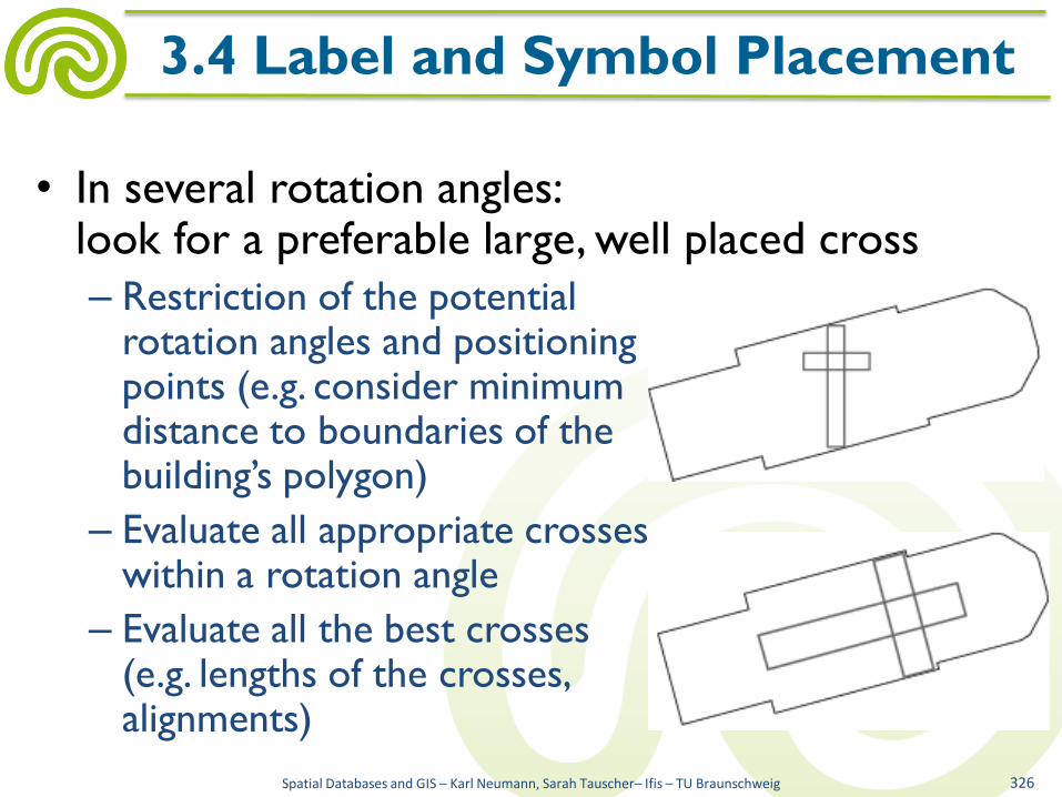
• In several rotation angles: look for a preferable large, well placed cross
– Restriction of the potential rotation angles and positioning points (e.g. consider minimum distance to boundaries of the building’s polygon)
– Evaluate all appropriate crosses within a rotation angle
– Evaluate all the best crosses (e.g. lengths of the crosses, alignments)
Spatial Databases and GIS – Karl Neumann, Sarah Tauscher– Ifis – TU Braunschweig 326
3.4 Label and Symbol Placement
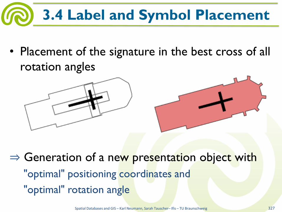
• Placement of the signature in the best cross of all
rotation angles
⇒ Generation of a new presentation object with
"optimal" positioning coordinates and
"optimal" rotation angle
Spatial Databases and GIS – Karl Neumann, Sarah Tauscher– Ifis – TU Braunschweig 327
3.4 Label and Symbol Placement

• Both methods applied to inventory data extracts
Spatial Databases and GIS – Karl Neumann, Sarah Tauscher– Ifis – TU Braunschweig 328
3.4 Label and Symbol Placement
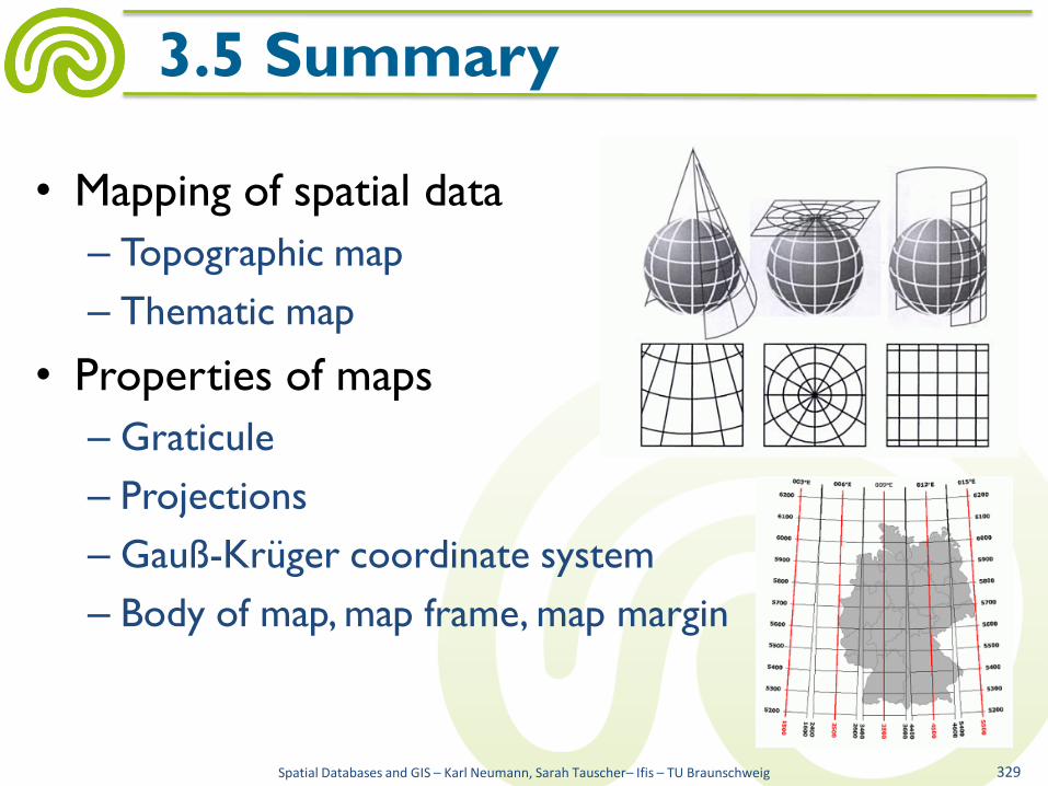
• Mapping of spatial data
– Topographic map
– Thematic map
• Properties of maps
– Graticule
– Projections
– Gauß-Krüger coordinate system
– Body of map, map frame, map margin
Spatial Databases and GIS – Karl Neumann, Sarah Tauscher– Ifis – TU Braunschweig 329
3.5 Summary

• Signatures, text, color
– Point signatures
– Line signatures
– Area signatures
– Derivation rules
– TK25, real estate map
• Geometric generalization
– Smoothing of polylines
– Simplification of polylines
Spatial Databases and GIS – Karl Neumann, Sarah Tauscher– Ifis – TU Braunschweig 330
3.5 Summary
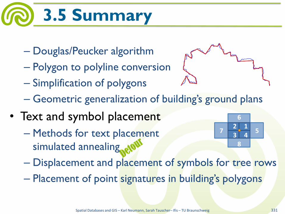
– Douglas/Peucker algorithm
– Polygon to polyline conversion
– Simplification of polygons
– Geometric generalization of building’s ground plans
• Text and symbol placement
– Methods for text placement
simulated annealing
– Displacement and placement of symbols for tree rows
– Placement of point signatures in building’s polygons
Spatial Databases and GIS – Karl Neumann, Sarah Tauscher– Ifis – TU Braunschweig 331
3.5 Summary
2
4 1
5
6
8
7 3

Spatial Databases and GIS – Karl Neumann, Sarah Tauscher– Ifis – TU Braunschweig 332
3.5 Summary
GIS graticule
map
text signatures
color
collect
manage
analyse
display
generalization
area labelling
simplifying lines
polygon→ line
design elements
placement
topographic
thematic
building signatures
tree rows as optimization problem


![Home [vivaldi-bs.de]vivaldi-bs.de/images/weekend_web.pdf · 2019. 2. 4. · Donald Russell - Rinderfilet mit Portweinsauce Ristorante . Weekend-Menü Jdkobsmuscheln mit PencheI-0rangensdIdt](https://static.fdocuments.net/doc/165x107/60cb1d064d22a35c38424852/home-vivaldi-bsdevivaldi-bsdeimagesweekendwebpdf-2019-2-4-donald.jpg)