
3 Geodesy, Datums, Map Projec- tions, and Coordinate Systems
67
3 Geodesy, Datums, Map Projec-tions and Coordinate Systems
IntroductionGeographic information systems are
different from other information systems because they contain spatial data. These spatial data include coordinates that define the location, shape, and extent of geo-graphic objects. To effectively use GIS, we must develop a clear understanding of how coordinate systems are established and how coordinates are measured. This chapter introduces geodesy, the science of measur-ing the shape of the Earth, and map projec-tions, the transformation of coordinate locations from the Earth’s curved surface onto flat maps.
Defining coordinates for the Earth’s surface is complicated by two main factors. First, most people best understand geogra-phy in a Cartesian coordinate system on a flat surface. Humans naturally perceive the Earth’s surface as flat, because at human scales the Earth’s curvature is barely per-ceptible. Humans have been using flat maps for more than 40 centuries, and although globes are quite useful for percep-tion and visualization at extremely small scales, they are not practical for most pur-poses.
A flat map must distort geometry in some way because the Earth is curved. When we plot latitude and longitude coor-dinates on a Cartesian system, “straight” lines will appear bent, and areas will be incorrect. This distortion may be difficult to detect on detailed maps that cover a small
area, but the distortion is quite apparent on large-area maps. Quantitative measure-ments on these maps are affected by the distortion, so we must somehow reconcile the mapping of a curved surface onto a flat surface.
The second main problem when defin-ing a coordinate system comes from the irregular nature of the Earth’s shape. We learn in our earliest geography lessons that the Earth is shaped as a sphere. This is a valid approximation for many uses, how-ever, it is only an approximation. Several forces in the present and past have resulted in an irregularly shaped Earth. These defor-mations affect how we best map the surface of the Earth, and how we define Cartesian coordinate systems for mapping and GIS.
Early Measurements Humans have long speculated on the
shape and size of the Earth. Babylonians believed the Earth was a flat disk floating in an endless ocean, a notion also adopted by Homer, one of the more widely known Greek writers. The Greeks were early champions of geometry, and they had many competing views of the shape of the Earth. One early Greek, Anaximenes, believed the Earth was a rectangular box, while Pythag-oras and later Aristotle reasoned that the Earth must be a sphere. This deduction was based on many lines of evidence, and also on a belief of divine direction by the gods.
68 GIS Fundamentals
Pythagoras believed the sphere was the most perfect geometric figure, and that the gods would use this perfect shape for their great-est creation. Aristotle also observed that ships disappeared over the horizon, the moon appeared to be a sphere, the stars moved in circular patterns, and noted reports from wandering fishermen on shifts in the constellations. These observations were all consistent with a spherical Earth.
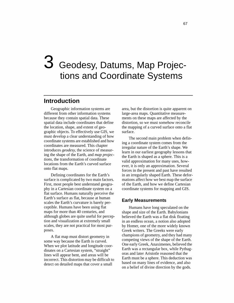
After scientific support for a spherical Earth became entrenched, Greek scientists turned toward estimating the size of the sphere. Eratosthenes, a Greek scholar in Egypt, performed one of the earliest well-founded measurements of the Earth’s cir-cumference. He noticed that on the summer solstice the sun at noon shone to the bottom of a deep well in Syene. He believed that the well was located on the Tropic of Cancer, so that the sun would be exactly overhead dur-ing the summer solstice. He also observed
that at exactly the same date and time a verti-cal post cast a shadow when located at Alex-andria, about 805 kilometers north. The shadow/post combination defined an angle which was about 7o12’, or about 1/50th of a circle (Figure 3-1).
Eratosthenes deduced that the Earth must be 805 multiplied by 50 or about 40,250 kilometers in circumference. His cal-culations were all in stadia, the unit of mea-sure of the time, and have been converted here to the metric equivalent, given our best idea of the length of a stadia. Eratosthenes’ estimate is close to our modern measurement of the Earth circumference of 38,762 kilo-meters. The difference is less than 4%.
The accuracy of Eratosthenes’ estimate is quite remarkable, given the equipment for measuring distance and angles at that time, and because a number of his assumptions were incorrect. The well at Syene was
Figure 3-1: Measurements made by Eratosthenes to determine the circumference of the Earth.
Chapter 3: Geodesy, Projections, and Coordinate Systems 69
located about 60 kilometers off the Tropic of Cancer, so the sun was not directly over-head. The true distance between the well location and Alexandria was about 729 kilo-meters, not 805, and the well was 3o3’ east of the meridian of Alexandria, and not due north. However these errors either compen-sated for or were offset by measurement errors to end up with an amazingly accurate estimate.
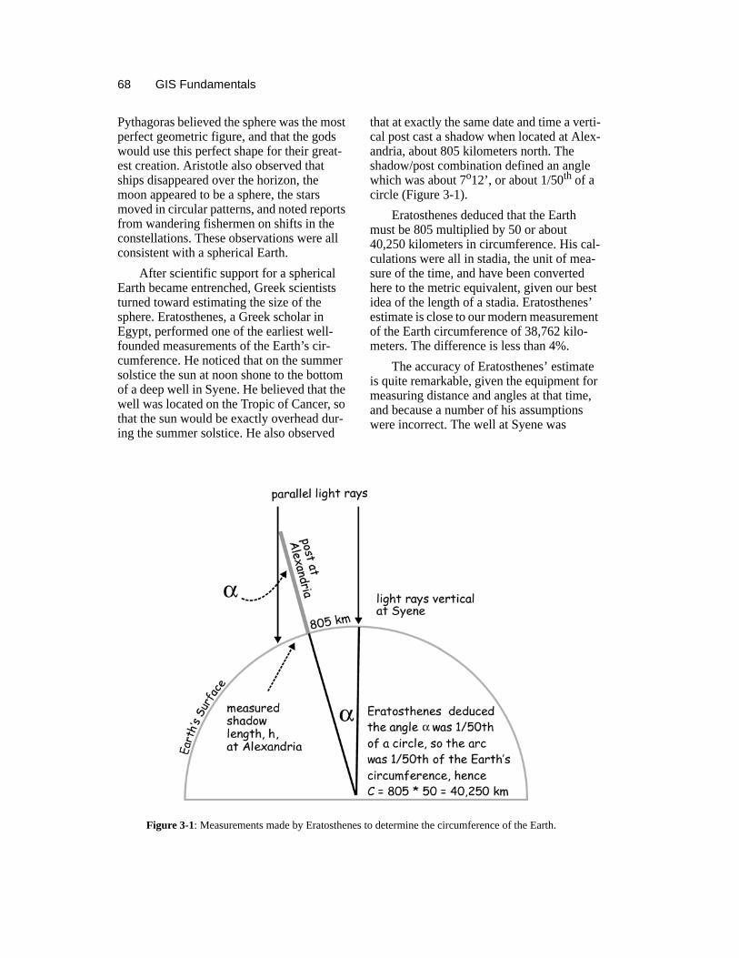
Posidonius made an independent esti-mate of the size of the Earth sphere by mea-suring angles to a star near the horizon (Figure 3-2). Stars visible in the night sky define a uniform reference. The angle between a local vertical line and a star loca-tion is called a zenith angle. The zenith angle may be measured simultaneously at two locations on Earth, and the difference
between the zenith angles used to calculate the circumference of the Earth. In Figure 3-2, the two zenith angles, α and γ, are mea-sured to a star. The surface distance between these two locations is also measured, and the measurements combined with geometric relationships to calculate the Earth circum-ference (Figure 3-2). Posidonius calculated the difference in the zenith angles to a known star as about 1/48th of a circle when measured at Rhodes and Alexandria. By estimating these two towns to be about 805 kilometers apart, he calculated the circum-ference of the Earth to be 38,600 kilometers. Again there were compensating errors, resulting in an accurate value. Another Greek scientist determined the circumfer-ence to be 28,960 kilometers, and unfortu-nately this shorter measurement was adopted
Figure 3-2: The Earth’s radius and circumference may be determined by simultaneous measurement of zenith angles at two points. Two points are separated by an arc distance a measured on the Earth surface. These points also span an angle θ defined at the Earth center. The local zenith angles α and γ are related to θ, and the Earth radius is related to a and θ. Once the radius is calculated, the Earth circumference may be determined.
70 GIS Fundamentals
by Ptolemy for his world maps. This esti-mate was widely accepted until the 1500s, when Gerardus Mercator revised the figure upward.
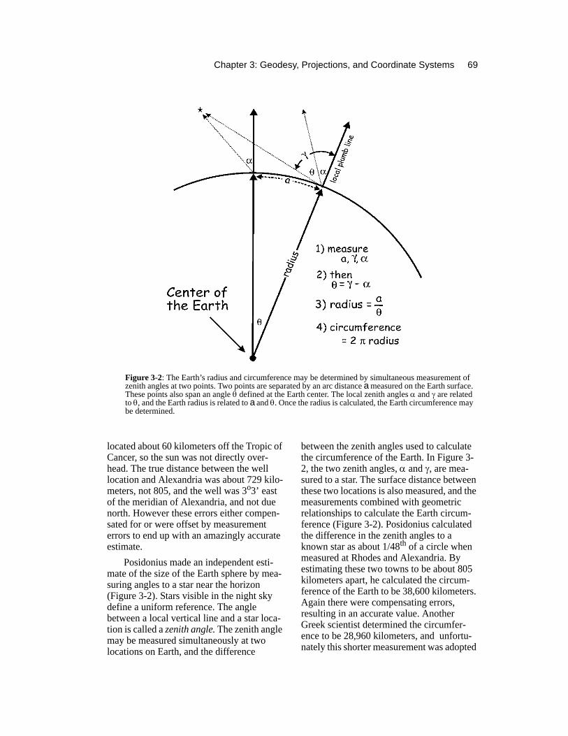
During the 17th and 18th centuries two developments led to intense activity directed at measuring the size and shape of the Earth. Sir Isaac Newton and others reasoned the Earth must be flattened somewhat due to rotational forces. They argued that centrifu-gal forces cause the equatorial regions of the Earth to bulge as it spins on its axis. They proposed the Earth would be better modeled by an ellipsoid, a sphere that was slightly flattened at the poles. Measurements by their French contemporaries taken north and south of Paris suggested the Earth was flat-tened in an equatorial direction and not in a polar direction. The controversy persisted until expeditions by the French Royal Acad-emy of Sciences between 1730 and 1745 measured the shape of the Earth near the Equator in South America and in the high northern latitudes of Europe. Complex, repeated, highly accurate measurements established the curvature of the Earth was greater at the Equator than the poles, and that an ellipsoid flattened at the poles was the best geometric model of the Earth’s sur-face.
Note that the words spheroid and ellip-soid are often used interchangeably. For example, the Clarke 1880 ellipsoid is often referred to as the Clarke 1880 spheroid, because Clarke provided parameters for an ellipsoidal model of the Earth’s shape. GIS software often prompts the user for a spher-oid when defining a coordinate projection, and then lists a set of ellipsoids for choices.
An ellipsoid is sometimes referred to as a special class of spheroid known as an “oblate” spheroid. Thus, it is less precise but still correct to refer to an ellipsoid more gen-erally as a spheroid. It would perhaps cause less confusion if the terms were used more consistently, but the usage is widespread. Ellipsoids are almost always used to model the Earth’s shape, and they are often referred to as spheroids.
Specifying the EllipsoidOnce the general shape of the Earth was
determined, geodesists focused on precisely measuring the size of the ellipsoid. The ellipsoid has two characteristic dimensions (Figure 3-3). These are the semi-major axis, the radius r1 in the Equatorial direction, and the semi-minor axis, the radius r2 in the polar direction. The equatorial radius is always greater than the polar radius for the Earth ellipsoid. This difference in polar and equatorial radii can also be described by the flattening factor, as shown in Figure 3-3.
Earth radii have been determined since the 18th century using a number of methods, and for many parts of the globe. The most common methods until recently have involved astronomical observations similar to the those performed by Posidonius. These astronomical observations, also called celes-tial observations, are combined with long-distance surveys over large areas. Star and sun locations have been observed and cata-loged for centuries, and combined with accurate clocks, the positions of these celes-tial bodies may be measured to precisely establish the latitudes and longitudes of
Figure 3-3: An ellipsoidal model of the Earth’s shape.
Chapter 3: Geodesy, Projections, and Coordinate Systems 71
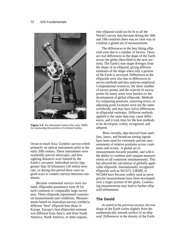
points on the surface of the Earth. Measure-ments during the 18th, 19th and early 20th centuries used optical instruments for celes-tial observations (Figure 3-4).
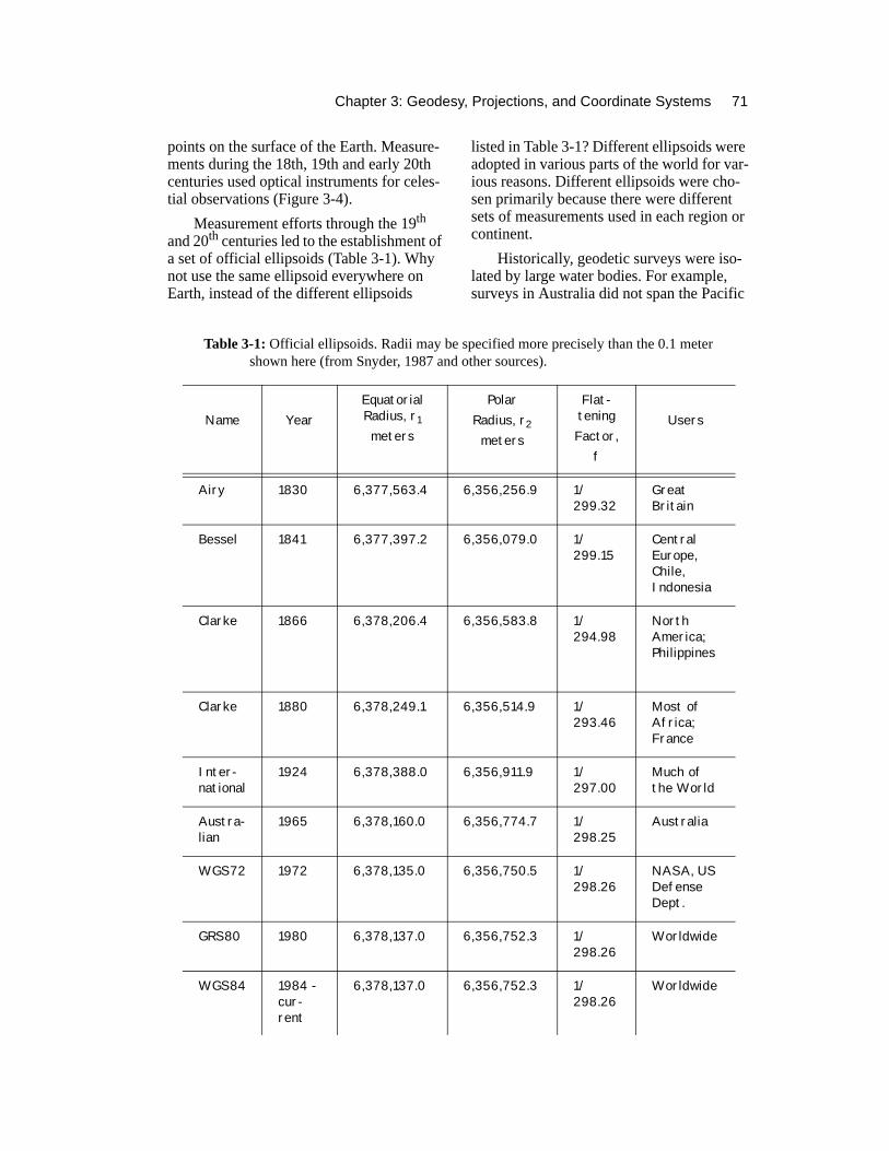
Measurement efforts through the 19th and 20th centuries led to the establishment of a set of official ellipsoids (Table 3-1). Why not use the same ellipsoid everywhere on Earth, instead of the different ellipsoids
listed in Table 3-1? Different ellipsoids were adopted in various parts of the world for var-ious reasons. Different ellipsoids were cho-sen primarily because there were different sets of measurements used in each region or continent.
Historically, geodetic surveys were iso-lated by large water bodies. For example, surveys in Australia did not span the Pacific
Table 3-1: Official ellipsoids. Radii may be specified more precisely than the 0.1 meter shown here (from Snyder, 1987 and other sources).
Name YearEquatorial Radius, r1meters
Polar Radius, r2
meters
Flat-teningFactor,
f
Users
Airy 1830 6,377,563.4 6,356,256.9 1/299.32
Great Britain
Bessel 1841 6,377,397.2 6,356,079.0 1/299.15
Central Europe, Chile, Indonesia
Clarke 1866 6,378,206.4 6,356,583.8 1/294.98
North America; Philippines
Clarke 1880 6,378,249.1 6,356,514.9 1/293.46
Most of Africa; France
Inter-national
1924 6,378,388.0 6,356,911.9 1/297.00
Much of the World
Austra-lian
1965 6,378,160.0 6,356,774.7 1/298.25
Australia
WGS72 1972 6,378,135.0 6,356,750.5 1/298.26
NASA, US Defense Dept.
GRS80 1980 6,378,137.0 6,356,752.3 1/298.26
Worldwide
WGS84 1984 - cur-rent
6,378,137.0 6,356,752.3 1/298.26
Worldwide
72 GIS Fundamentals
Ocean to reach Asia. Geodetic surveys relied primarily on optical instruments prior to the early 20th century. These instruments were essentially precise telescopes, and thus sighting distances were limited by the Earth’s curvature. Individual survey legs greater than 50 kilometers (30 miles) were rare, so during this period there were no good ways to connect surveys between con-tinents.
Because continental surveys were iso-lated, ellipsoidal parameters were fit for each continent or comparably large survey area. These ellipsoids represented continen-tal measurements and conditions. Measure-ments based on Australian surveys yielded a different “best” ellipsoid than those in Europe. Europe’s best ellipsoidal estimate was different from Asia’s, and from South America, North America, or other regions.
One ellipsoid could not be fit to all the World’s survey data because during the 18th and 19th centuries there was no clear way to combine a global set of measurements.
The differences in the best fitting ellip-soid were due to a number of factors. There are real differences in the shape of the Earth across the globe (described in the next sec-tion). The Earth’s true shape diverges from the shape of an ellipsoid, giving different estimates of the shape when only a portion of the Earth is surveyed. Differences in the ellipsoids were also due to differences in survey methods and data analyses employed. Computational resources, the sheer number of survey points, and the scarcity of survey points for many areas were barriers to the development of global ellipsoids. Methods for computing positions, removing errors, or adjusting point locations were not the same worldwide, and may have led to differences in ellipsoidal estimates. Different methods applied to the same data may cause differ-ences, and it took time for the best methods to be developed, widely recognized, and adopted.
More recently, data derived from satel-lites, lasers, and broadcast timing signals have been used for extremely precise mea-surements of relative positions across conti-nents and oceans. A global set of measurements became possible, and with it the ability to combine and compare measure-ments on all continents simultaneously. This has allowed the calculation of globally appli-cable ellipsoids. Internationally recognized ellipsoids such as WGS72, GRS80, or WGS84 have become widely used as more precise measurements have been developed over a larger portion of the globe. Continu-ing measurements may lead to further ellip-soid refinements.
The GeoidAs noted in the previous section, the true
shape of the Earth varies slightly from the mathematically smooth surface of an ellip-soid. Differences in the density of the Earth
Figure 3-4: An instrument used in the early 1900s for measuring the position of celestial bodies.

Chapter 3: Geodesy, Projections, and Coordinate Systems 73
cause variation in the strength of the gravita-tional pull, in turn causing regions to dip or bulge above or below a reference ellipsoid. This undulating shape is called a geoid.
Geodesists have defined the geoid as the three-dimensional surface along which the pull of gravity is a specified constant. The geoidal surface may be thought of as the level of an imaginary sea, were it to cover the entire Earth and not be affected by wind, waves, the moon, or forces other than grav-ity. The surface of the geoid is in this way related to mean sea level, or other references against which heights are measured. Geode-sists may measure surface heights relative to the geoid, and at any point on Earth there are three important surfaces, the ellipsoid, the geoid, and the Earth surface (Figure 3-5).
Because we have two reference sur-faces, a geiod and an ellipsoid, we also have two bases from which to measure height. Elevation is typically defined as the vertical distance above a geoid. This height above a geoid is also called the orthometric height. Orthometric heights are the basis for eleva-tion measurements. Heights above the ellip-soid are often referred to as an ellipsoidal height. These are illustrated in Figure 3-5, with the ellipsoidal height labeled h, and
orthometric height labeled H. The differ-ence, shown in the figure as N, has various names, including geoidal height and geoidal separation.
Geoidal variation in the Earth’s shape is the main cause for different ellipsoids being employed in different parts of the world. The best local fit of an ellipsoid to the geoidal surface in one portion of the globe may not be the best fit in another portion. This is illustrated in Figure 3-6. Ellipsoid A fits well over one portion of the geoid, ellipsoid B in another, but both provide a poor fit in many other areas of the Earth’s surface. Initial measurements were often localized, so the deviations in other parts of the Earth were up to several hundred meters. A global array of measurements allows the estimation of a globally optimal ellipsoid.
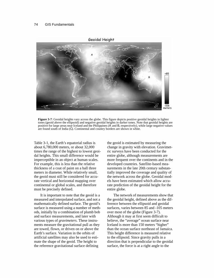
The geoid varies by less than 100 meters from the ellipsoid over most of the Earth (Figure 3-7), and these differences between the geoid and the ellipsoid are small relative to the differences between an ellipsoidal and a spherical model. The separation between the geoid and ellipsoid represented by the geoidal heights is also quite small relative to the polar and equatorial radii. As noted in
Figure 3-5: Ellipsoidal, orthometric, and geoidal height are interrelated. Note that values for N are highly exagerated in this figure - undulations are typically much less than differences in H.
Figure 3-6: Locally fit ellipsoids may provide poor fits in other portions of the Earth’s surface.
74 GIS Fundamentals
Table 3-1, the Earth’s equatorial radius is about 6,780,000 meters, or about 32,000 times the range of the highest to lowest geoi-dal heights. This small difference would be imperceptible in an object at human scales. For example, this is less than the relative thickness of a coat of paint on a ball three meters in diameter. While relatively small, the geoid must still be considered for accu-rate vertical and horizontal mapping over continental or global scales, and therefore must be precisely defined.
It is important to note that the geoid is a measured and interpolated surface, and not a mathematically defined surface. The geoid’s surface is measured using a number of meth-ods, initially by a combination of plumb bob and surface measurements, and later with various types of gravimeters. These instru-ments measure the gravitational pull as they are towed, flown, or driven on or above the Earth’s surface. Variation in the orbits of artificial satellites may also be used to esti-mate the shape of the geoid. The height to the reference gravitational surface defining
the geoid is estimated by measuring the change in gravity with elevation. Gravimet-ric surveys have been conducted for the entire globe, although measurements are more frequent over the continents and in the developed countries. Satellite-based mea-surements in the late 20th century substan-tially improved the coverage and quality of the network across the globe. Geoidal mod-els have been estimated which allow accu-rate prediction of the geoidal height for the entire globe.
The network of measurements show that the geoidal height, defined above as the dif-ference between the ellipsoid and geoidal surfaces, varies between 85 and -105 meters over most of the globe (Figure 3-7). Although it may at first seem difficult to believe, the “average” ocean surface near Iceland is more than 150 meters “higher” than the ocean surface northeast of Jamaica. This height difference is measured relative to the ellipsoid. Since gravity pulls in a direction that is perpendicular to the geoidal surface, the force is at a right angle to the
Figure 3-7: Geoidal heights vary across the globe. This figure depicts positive geoidal heights in lighter tones (geoid above the ellipsoid) and negative geoidal heights in darker tones. Note that geoidal heights are positive for large areas near Iceland and the Philippines (A and B, respectively), while large negative values are found south of India (C). Continental and country borders are shown in white.
Chapter 3: Geodesy, Projections, and Coordinate Systems 75
surface of the ocean, resulting in permanent bulges and dips in the mean ocean surface. Variation in ocean heights due to swells and wind-driven waves are more apparent at local scales, but are much smaller than the long-distance geoidal undulations.
Geographic Coordinates, Lati-tude, and Longitude
Once a size and shape of the reference ellipsoid has been determined, the poles and Equator are also defined. The poles are defined by the axis of revolution of the ellip-soid, and the Equator is defined as the circle mid-way between the two poles, at a right angle to the polar axis, and spanning the widest dimension of the ellipsoid. We now must go about defining a coordinate grid, a reference system by which we may specify the position of features on the ellipsoidal surface.
A geographic coordinate system has been defined for the Earth with reference to
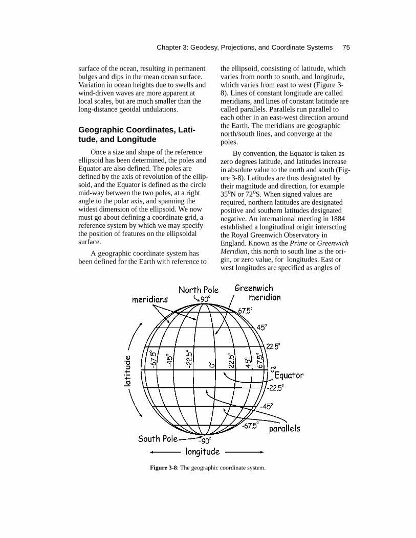
the ellipsoid, consisting of latitude, which varies from north to south, and longitude, which varies from east to west (Figure 3-8). Lines of constant longitude are called meridians, and lines of constant latitude are called parallels. Parallels run parallel to each other in an east-west direction around the Earth. The meridians are geographic north/south lines, and converge at the poles.
By convention, the Equator is taken as zero degrees latitude, and latitudes increase in absolute value to the north and south (Fig-ure 3-8). Latitudes are thus designated by their magnitude and direction, for example 35oN or 72oS. When signed values are required, northern latitudes are designated positive and southern latitudes designated negative. An international meeting in 1884 established a longitudinal origin interscting the Royal Greenwich Observatory in England. Known as the Prime or Greenwich Meridian, this north to south line is the ori-gin, or zero value, for longitudes. East or west longitudes are specified as angles of
Figure 3-8: The geographic coordinate system.
76 GIS Fundamentals
rotation away from the Prime Meridian. When required, west is considered negative and east positive.
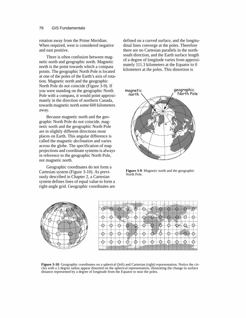
There is often confusion between mag-netic north and geographic north. Magnetic north is the point towards which a compass points. The geographic North Pole is located at one of the poles of the Earth’s axis of rota-tion. Magnetic north and the geographic North Pole do not coincide (Figure 3-9). If you were standing on the geographic North Pole with a compass, it would point approxi-mately in the direction of northern Canada, towards magnetic north some 600 kilometers away.
Because magnetic north and the geo-graphic North Pole do not coincide, mag-netic north and the geographic North Pole are in slightly different directions most places on Earth. This angular difference is called the magnetic declination and varies across the globe. The specification of map projections and coordinate systems is always in reference to the geographic North Pole, not magnetic north.
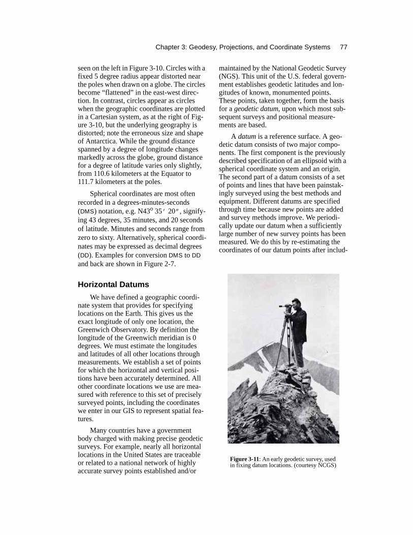
Geographic coordinates do not form a Cartesian system (Figure 3-10). As previ-ously described in Chapter 2, a Cartesian system defines lines of equal value to form a right-angle grid. Geographic coordinates are
defined on a curved surface, and the longitu-dinal lines converge at the poles. Therefore there are no Cartesian parallels in the north-south direction, and the Earth surface length of a degree of longitude varies from approxi-mately 111.3 kilometers at the Equator to 0 kilometers at the poles. This distortion is
Figure 3-10: Geographic coordinates on a spherical (left) and Cartesian (right) representation. Notice the cir-cles with a 5 degree radius appear distorted on the spherical representation, illustrating the change in surface distance represented by a degree of longitude from the Equator to near the poles.
Figure 3-9: Magnetic north and the geographic North Pole.
Chapter 3: Geodesy, Projections, and Coordinate Systems 77
seen on the left in Figure 3-10. Circles with a fixed 5 degree radius appear distorted near the poles when drawn on a globe. The circles become “flattened” in the east-west direc-tion. In contrast, circles appear as circles when the geographic coordinates are plotted in a Cartesian system, as at the right of Fig-ure 3-10, but the underlying geography is distorted; note the erroneous size and shape of Antarctica. While the ground distance spanned by a degree of longitude changes markedly across the globe, ground distance for a degree of latitude varies only slightly, from 110.6 kilometers at the Equator to 111.7 kilometers at the poles.
Spherical coordinates are most often recorded in a degrees-minutes-seconds (DMS) notation, e.g. N43o 35’ 20”, signify-ing 43 degrees, 35 minutes, and 20 seconds of latitude. Minutes and seconds range from zero to sixty. Alternatively, spherical coordi-nates may be expressed as decimal degrees (DD). Examples for conversion DMS to DD and back are shown in Figure 2-7.
Horizontal DatumsWe have defined a geographic coordi-
nate system that provides for specifying locations on the Earth. This gives us the exact longitude of only one location, the Greenwich Observatory. By definition the longitude of the Greenwich meridian is 0 degrees. We must estimate the longitudes and latitudes of all other locations through measurements. We establish a set of points for which the horizontal and vertical posi-tions have been accurately determined. All other coordinate locations we use are mea-sured with reference to this set of precisely surveyed points, including the coordinates we enter in our GIS to represent spatial fea-tures.
Many countries have a government body charged with making precise geodetic surveys. For example, nearly all horizontal locations in the United States are traceable or related to a national network of highly accurate survey points established and/or
maintained by the National Geodetic Survey (NGS). This unit of the U.S. federal govern-ment establishes geodetic latitudes and lon-gitudes of known, monumented points. These points, taken together, form the basis for a geodetic datum, upon which most sub-sequent surveys and positional measure-ments are based.
A datum is a reference surface. A geo-detic datum consists of two major compo-nents. The first component is the previously described specification of an ellipsoid with a spherical coordinate system and an origin. The second part of a datum consists of a set of points and lines that have been painstak-ingly surveyed using the best methods and equipment. Different datums are specified through time because new points are added and survey methods improve. We periodi-cally update our datum when a sufficiently large number of new survey points has been measured. We do this by re-estimating the coordinates of our datum points after includ-
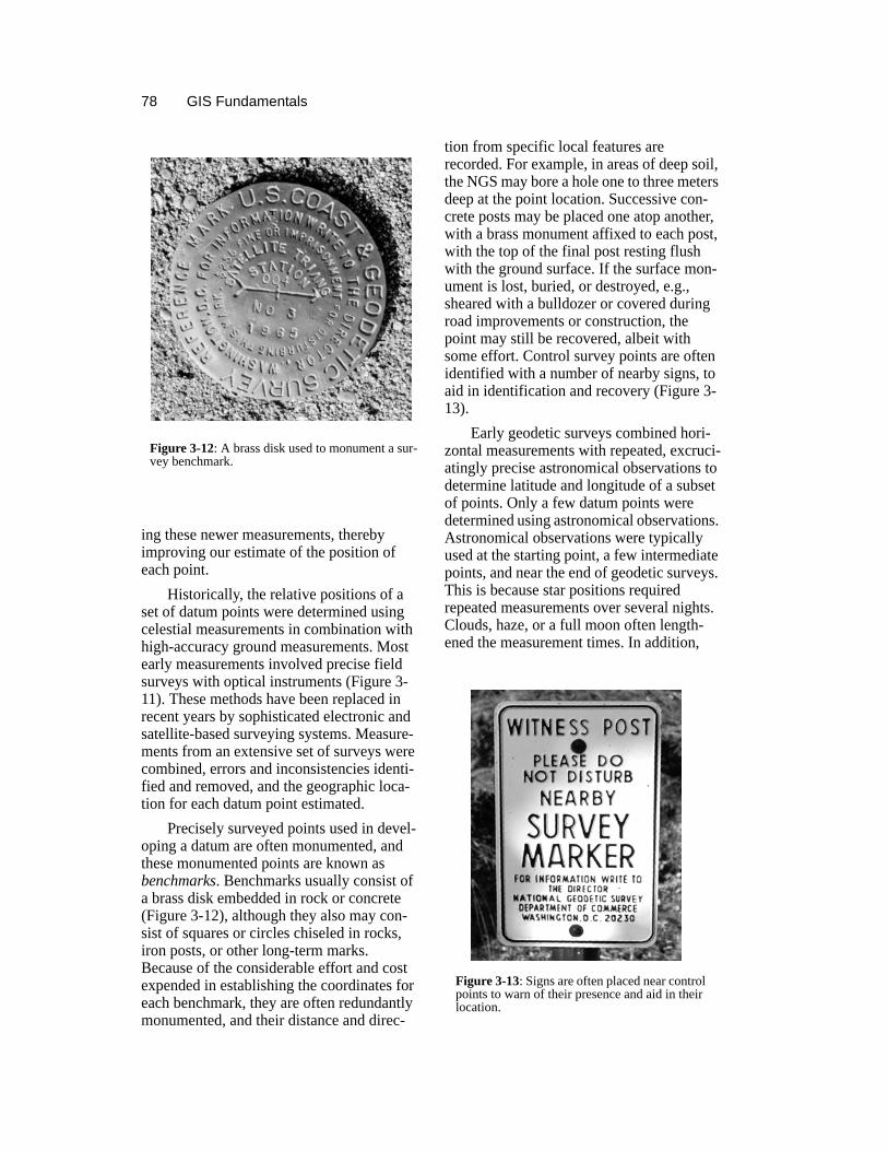
Figure 3-11: An early geodetic survey, used in fixing datum locations. (courtesy NCGS)
78 GIS Fundamentals
ing these newer measurements, thereby improving our estimate of the position of each point.
Historically, the relative positions of a set of datum points were determined using celestial measurements in combination with high-accuracy ground measurements. Most early measurements involved precise field surveys with optical instruments (Figure 3-11). These methods have been replaced in recent years by sophisticated electronic and satellite-based surveying systems. Measure-ments from an extensive set of surveys were combined, errors and inconsistencies identi-fied and removed, and the geographic loca-tion for each datum point estimated.
Precisely surveyed points used in devel-oping a datum are often monumented, and these monumented points are known as benchmarks. Benchmarks usually consist of a brass disk embedded in rock or concrete (Figure 3-12), although they also may con-sist of squares or circles chiseled in rocks, iron posts, or other long-term marks. Because of the considerable effort and cost expended in establishing the coordinates for each benchmark, they are often redundantly monumented, and their distance and direc-
tion from specific local features are recorded. For example, in areas of deep soil, the NGS may bore a hole one to three meters deep at the point location. Successive con-crete posts may be placed one atop another, with a brass monument affixed to each post, with the top of the final post resting flush with the ground surface. If the surface mon-ument is lost, buried, or destroyed, e.g., sheared with a bulldozer or covered during road improvements or construction, the point may still be recovered, albeit with some effort. Control survey points are often identified with a number of nearby signs, to aid in identification and recovery (Figure 3-13).
Early geodetic surveys combined hori-zontal measurements with repeated, excruci-atingly precise astronomical observations to determine latitude and longitude of a subset of points. Only a few datum points were determined using astronomical observations. Astronomical observations were typically used at the starting point, a few intermediate points, and near the end of geodetic surveys. This is because star positions required repeated measurements over several nights. Clouds, haze, or a full moon often length-ened the measurement times. In addition,
Figure 3-12: A brass disk used to monument a sur-vey benchmark.
Figure 3-13: Signs are often placed near control points to warn of their presence and aid in their location.
Chapter 3: Geodesy, Projections, and Coordinate Systems 79
celestial measurements required correction for atmospheric refraction, a process which bends light and changes the apparent posi-tion of stars. Refraction depends on how high the star is in the sky at the time of mea-surement, as well as temperature, atmo-spheric humidity, and other factors.
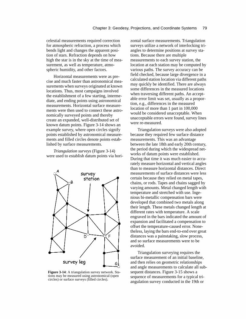
Horizontal measurements were as pre-cise and much faster than astronomical mea-surements when surveys originated at known locations. Thus, most campaigns involved the establishment of a few starting, interme-diate, and ending points using astronomical measurements. Horizontal surface measure-ments were then used to connect these astro-nomically surveyed points and thereby create an expanded, well-distributed set of known datum points. Figure 3-14 shows an example survey, where open circles signify points established by astronomical measure-ments and filled circles denote points estab-lished by surface measurements.
Triangulation surveys (Figure 3-14) were used to establish datum points via hori-
zontal surface measurements. Triangulation surveys utilize a network of interlocking tri-angles to determine positions at survey sta-tions. Because there are multiple measurements to each survey station, the location at each station may be computed by various paths. The survey accuracy can be field checked, because large divergence in a calculated station location via different paths may quickly be identified. There are always some differences in the measured locations when traversing different paths. An accept-able error limit was set, usually as a propor-tion, e.g., differences in the measured location of more than 1 part in 100,000 would be considered unacceptable. When unacceptable errors were found, survey lines were re-measured.
Triangulation surveys were also adopted because they required few surface distance measurements. This was an advantage between the late 18th and early 20th century, the period during which the widespread net-works of datum points were established. During that time it was much easier to accu-rately measure horizontal and vertical angles than to measure horizontal distances. Direct measurements of surface distances were less certain because they relied on metal tapes, chains, or rods. Tapes and chains sagged by varying amounts. Metal changed length with temperature and stretched with use. Inge-nious bi-metallic compensation bars were developed that combined two metals along their length. These metals changed length at different rates with temperature. A scale engraved in the bars indicated the amount of expansion and facilitated a compensation to offset the temperature-caused error. None-theless, laying the bars end-to-end over great distances was a painstaking, slow process, and so surface measurements were to be avoided.
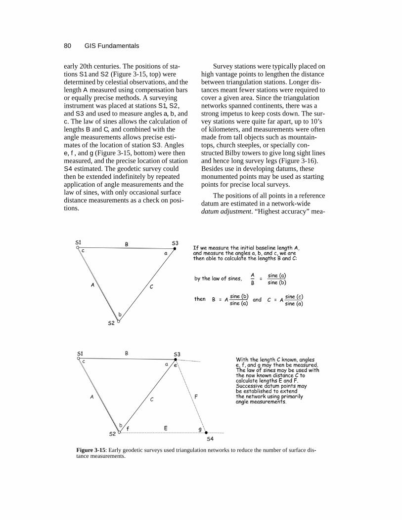
Triangulation surveying requires the surface measurement of an initial baseline, and then relies on geometric relationships and angle measurements to calculate all sub-sequent distances. Figure 3-15 shows a sequence of measurements for a typical tri-angulation survey conducted in the 19th or
Figure 3-14: A triangulation survey network. Sta-tions may be measured using astronomical (open circles) or surface surveys (filled circles).
80 GIS Fundamentals
early 20th centuries. The positions of sta-tions S1 and S2 (Figure 3-15, top) were determined by celestial observations, and the length A measured using compensation bars or equally precise methods. A surveying instrument was placed at stations S1, S2, and S3 and used to measure angles a, b, and c. The law of sines allows the calculation of lengths B and C, and combined with the angle measurements allows precise esti-mates of the location of station S3. Angles e, f, and g (Figure 3-15, bottom) were then measured, and the precise location of station S4 estimated. The geodetic survey could then be extended indefinitely by repeated application of angle measurements and the law of sines, with only occasional surface distance measurements as a check on posi-tions.
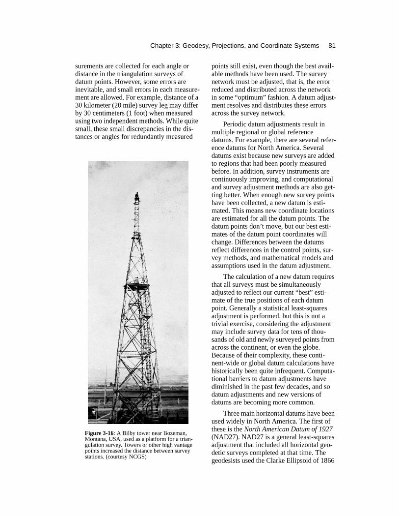
Survey stations were typically placed on high vantage points to lengthen the distance between triangulation stations. Longer dis-tances meant fewer stations were required to cover a given area. Since the triangulation networks spanned continents, there was a strong impetus to keep costs down. The sur-vey stations were quite far apart, up to 10’s of kilometers, and measurements were often made from tall objects such as mountain-tops, church steeples, or specially con-structed Bilby towers to give long sight lines and hence long survey legs (Figure 3-16). Besides use in developing datums, these monumented points may be used as starting points for precise local surveys.
The positions of all points in a reference datum are estimated in a network-wide datum adjustment. “Highest accuracy” mea-
Figure 3-15: Early geodetic surveys used triangulation networks to reduce the number of surface dis-tance measurements.
Chapter 3: Geodesy, Projections, and Coordinate Systems 81
surements are collected for each angle or distance in the triangulation surveys of datum points. However, some errors are inevitable, and small errors in each measure-ment are allowed. For example, distance of a 30 kilometer (20 mile) survey leg may differ by 30 centimeters (1 foot) when measured using two independent methods. While quite small, these small discrepancies in the dis-tances or angles for redundantly measured
points still exist, even though the best avail-able methods have been used. The survey network must be adjusted, that is, the error reduced and distributed across the network in some “optimum” fashion. A datum adjust-ment resolves and distributes these errors across the survey network.
Periodic datum adjustments result in multiple regional or global reference datums. For example, there are several refer-ence datums for North America. Several datums exist because new surveys are added to regions that had been poorly measured before. In addition, survey instruments are continuously improving, and computational and survey adjustment methods are also get-ting better. When enough new survey points have been collected, a new datum is esti-mated. This means new coordinate locations are estimated for all the datum points. The datum points don’t move, but our best esti-mates of the datum point coordinates will change. Differences between the datums reflect differences in the control points, sur-vey methods, and mathematical models and assumptions used in the datum adjustment.
The calculation of a new datum requires that all surveys must be simultaneously adjusted to reflect our current “best” esti-mate of the true positions of each datum point. Generally a statistical least-squares adjustment is performed, but this is not a trivial exercise, considering the adjustment may include survey data for tens of thou-sands of old and newly surveyed points from across the continent, or even the globe. Because of their complexity, these conti-nent-wide or global datum calculations have historically been quite infrequent. Computa-tional barriers to datum adjustments have diminished in the past few decades, and so datum adjustments and new versions of datums are becoming more common.
Three main horizontal datums have been used widely in North America. The first of these is the North American Datum of 1927 (NAD27). NAD27 is a general least-squares adjustment that included all horizontal geo-detic surveys completed at that time. The geodesists used the Clarke Ellipsoid of 1866
Figure 3-16: A Bilby tower near Bozeman, Montana, USA, used as a platform for a trian-gulation survey. Towers or other high vantage points increased the distance between survey stations. (courtesy NCGS)
82 GIS Fundamentals
and held fixed the latitude and longitude of a survey station in Kansas. NAD27 yielded adjusted latitudes and longitudes for approx-imately 26,000 survey stations in the United States and Canada.
The North American Datum of 1983 (NAD83) is the immediate successor datum to NAD27. It was undertaken by the National Coast and Geodetic Survey to include the large number of geodetic survey points established between the mid-1920s and the early 1980s. Approximately 250,000 stations and 2,000,000 distance measure-ments were included in the adjustment. The GRS80 ellipsoid was used as reference. NAD83 uses an Earth-centered reference, rather than the fixed station selected for NAD27.
The World Geodetic System of 1984 (WGS84) is also commonly used, and was developed by the U.S. Department of Defense (DOD). It was developed in 1987 based on Doppler satellite measurements of the Earth, and is the base system used in most DOD maps and positional data. WGS84 has been updated based on more recent satellite measurements and is speci-fied using a version designator, e.g., the update based on data collected up to January 1994 is designated as WGS84 (G370). The WGS84 ellipsoid is very similar to the GRS80 ellipsoid.
Since different datums are based on dif-ferent sets of measurements and ellipsoids, the coordinates for benchmark datum points typically differ between datums. That is to say, the latitude and longitude location of a given benchmark in the NAD27 datum will likely be different from the latitude and lon-gitude of that same benchmark in the NAD83 or WGS84 datums. This is described as a datum shift. The monumented points do not move. Physically, the points remain in the same location; our estimates of the point locations change. As survey mea-surements improve through time, and there are more of them, we obtain better estimates of the true locations of the monumented datum points.
Coordinates across different datums may differ slightly, because of the differ-ences in the ellipsoid and in the measure-ments and methods used to estimate the locations of datum points. Differences may be small, e.g., the shift in coordinate loca-tions from WGS84 to NAD83 is often less than a meter, but shifts may be quite large. Care should be taken to not mix spatial data across datums unless the magnitude for the datum shift has been established for the area of interest, and this magnitude is considered small relative to overall data use and accu-racy specifications.
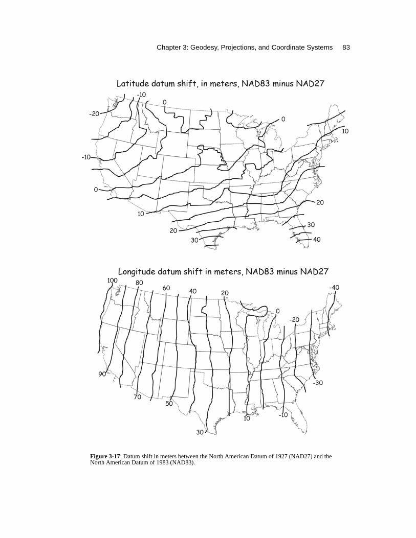
Datum shifts between NAD27 and NAD83 are often quite large, up to 100's of meters. Figure 3-17 indicates the relative size of shifts across the country between NAD27 and NAD83, based on estimates provided by the National Geodetic Survey. Notice that datum shifts between NAD27 and NAD83 are approximately -20 to 40 meters (70 to 140 feet) northward and between -40 and 100 meters (140 to 330 feet) east-west.
You should note that there are several versions of NAD83. Geodesists at the U.S. National Geodetic Survey find they have enough improved measurements of datum points to perform a complete network re-adjustment every five to ten years. Each re-adjustment combines the new measurements with older measurements in a least squares model, and distributes new, smaller esti-mates of error across the entire network of datum points. Therefore, there is typically a datum year and version associated with a set of benchmark coordinates, e.g., coordinates may be provided for a point with reference to the datum NAD83 (1986), or with refer-ence to NAD83 (1996). Distances of the shifts due to re-adjustments are typically less than one-half meter, and therefore they are often small relative to other positional uncer-tainties inherent in much spatial data. How-ever, these distances can be significant in many projects, and even if not, they may be cause for confusion unless their source is understood. Because of datum shifts due to the re-adjustments, for example, from
Chapter 3: Geodesy, Projections, and Coordinate Systems 83
Figure 3-17: Datum shift in meters between the North American Datum of 1927 (NAD27) and the North American Datum of 1983 (NAD83).
84 GIS Fundamentals
NAD27 to NAD83, or due to differences in subsequent versions of NAD83, it is impor-tant to note the datum underpinning a GIS development effort. If source data or maps are referenced to different datums, then they must be converted before they will overlay correctly.
Vertical DatumsJust as there are networks of well-mea-
sured points to define horizontal position, there are networks of points to define verti-cal datums. Vertical datums are used as a ref-erence for specifying heights. Much like horizontal datums, they are established through a set of painstakingly surveyed con-trol points. These point elevations are pre-cisely measured, initially through a set of optical surface measurements, but more recently using GPS, laser, satellite, and other measurement systems.
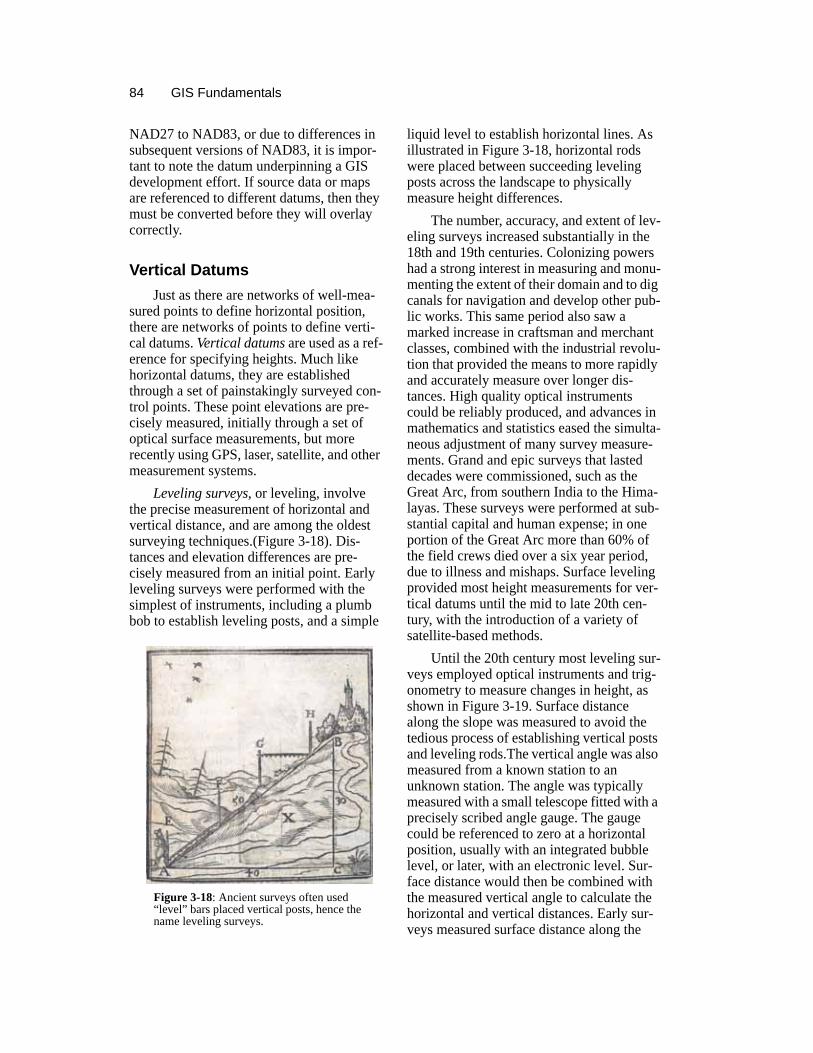
Leveling surveys, or leveling, involve the precise measurement of horizontal and vertical distance, and are among the oldest surveying techniques.(Figure 3-18). Dis-tances and elevation differences are pre-cisely measured from an initial point. Early leveling surveys were performed with the simplest of instruments, including a plumb bob to establish leveling posts, and a simple
liquid level to establish horizontal lines. As illustrated in Figure 3-18, horizontal rods were placed between succeeding leveling posts across the landscape to physically measure height differences.
The number, accuracy, and extent of lev-eling surveys increased substantially in the 18th and 19th centuries. Colonizing powers had a strong interest in measuring and monu-menting the extent of their domain and to dig canals for navigation and develop other pub-lic works. This same period also saw a marked increase in craftsman and merchant classes, combined with the industrial revolu-tion that provided the means to more rapidly and accurately measure over longer dis-tances. High quality optical instruments could be reliably produced, and advances in mathematics and statistics eased the simulta-neous adjustment of many survey measure-ments. Grand and epic surveys that lasted decades were commissioned, such as the Great Arc, from southern India to the Hima-layas. These surveys were performed at sub-stantial capital and human expense; in one portion of the Great Arc more than 60% of the field crews died over a six year period, due to illness and mishaps. Surface leveling provided most height measurements for ver-tical datums until the mid to late 20th cen-tury, with the introduction of a variety of satellite-based methods.
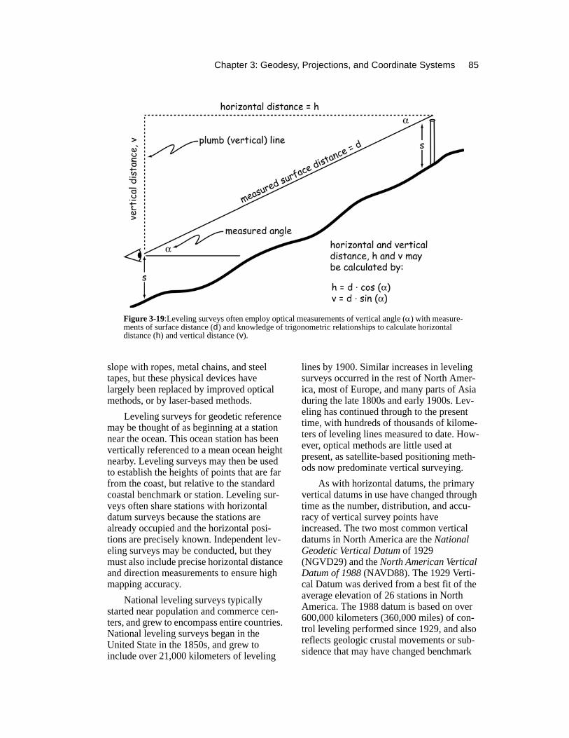
Until the 20th century most leveling sur-veys employed optical instruments and trig-onometry to measure changes in height, as shown in Figure 3-19. Surface distance along the slope was measured to avoid the tedious process of establishing vertical posts and leveling rods.The vertical angle was also measured from a known station to an unknown station. The angle was typically measured with a small telescope fitted with a precisely scribed angle gauge. The gauge could be referenced to zero at a horizontal position, usually with an integrated bubble level, or later, with an electronic level. Sur-face distance would then be combined with the measured vertical angle to calculate the horizontal and vertical distances. Early sur-veys measured surface distance along the
Figure 3-18: Ancient surveys often used “level” bars placed vertical posts, hence the name leveling surveys.
Chapter 3: Geodesy, Projections, and Coordinate Systems 85
slope with ropes, metal chains, and steel tapes, but these physical devices have largely been replaced by improved optical methods, or by laser-based methods.
Leveling surveys for geodetic reference may be thought of as beginning at a station near the ocean. This ocean station has been vertically referenced to a mean ocean height nearby. Leveling surveys may then be used to establish the heights of points that are far from the coast, but relative to the standard coastal benchmark or station. Leveling sur-veys often share stations with horizontal datum surveys because the stations are already occupied and the horizontal posi-tions are precisely known. Independent lev-eling surveys may be conducted, but they must also include precise horizontal distance and direction measurements to ensure high mapping accuracy.
National leveling surveys typically started near population and commerce cen-ters, and grew to encompass entire countries. National leveling surveys began in the United State in the 1850s, and grew to include over 21,000 kilometers of leveling
lines by 1900. Similar increases in leveling surveys occurred in the rest of North Amer-ica, most of Europe, and many parts of Asia during the late 1800s and early 1900s. Lev-eling has continued through to the present time, with hundreds of thousands of kilome-ters of leveling lines measured to date. How-ever, optical methods are little used at present, as satellite-based positioning meth-ods now predominate vertical surveying.
As with horizontal datums, the primary vertical datums in use have changed through time as the number, distribution, and accu-racy of vertical survey points have increased. The two most common vertical datums in North America are the National Geodetic Vertical Datum of 1929 (NGVD29) and the North American Vertical Datum of 1988 (NAVD88). The 1929 Verti-cal Datum was derived from a best fit of the average elevation of 26 stations in North America. The 1988 datum is based on over 600,000 kilometers (360,000 miles) of con-trol leveling performed since 1929, and also reflects geologic crustal movements or sub-sidence that may have changed benchmark
Figure 3-19:Leveling surveys often employ optical measurements of vertical angle (α) with measure-ments of surface distance (d) and knowledge of trigonometric relationships to calculate horizontal distance (h) and vertical distance (v).
86 GIS Fundamentals
elevation. NAVD88 adjusted the estimate of mean sea level slightly. Differences are observed when comparing NGVD29 and NAVD88 elevations for the same bench-marks.
Control Accuracy and Mainte-nance
In most cases the datum control points are too sparse to be sufficient for all needs in GIS data development. For example, precise point locations may be required when setting up a GPS receiving station, to georegister a scanned photograph or other imagery, or as the basis for a detailed subdivision or high-way survey. It is unlikely there will be more than one or two datum points within the work area for each of these activities. In many instances a denser network of known points is desirable. The monumented, pre-cisely determined point locations that are part of a datum may be used as a starting point for additional surveying. These smaller area surveys increase the density of precisely known points. The quality of the point loca-tions depends on the quality of the interven-ing survey, and a set of standards has been established for reporting survey quality.
The Federal Geodetic Control Commit-tee of the United States (FGCC) has pub-lished a detailed set of survey accuracy specifications. These specifications set a minimum acceptable accuracy for surveys and establish procedures and protocols to ensure the advertised accuracy has been obtained. The FGCC specifications establish a hierarchy of accuracy. First order survey measurements are accurate to within 1 part in 100,000. This means the error of the sur-vey is no larger than one unit of measure for each 100,000 units of distance surveyed. The maximum horizontal measurement error of a 5,000 meter baseline (about 3 miles) would be no larger than 5 centimeters (about 2
inches). Accuracies are specified by Class and Orders, down to a Class III, 2nd order point with an error of no more than 1 part in 5,000.
Federal, state, provincial, and county surveyors typically have a set of identified points that have been precisely surveyed to augment the local control network. The accuracy of these points is usually available, and point description and location may be obtained from the appropriate surveying authority.
The U.S. NGS maintains and dissemi-nates a list of control points, including those points used in datum definitions and adjust-ment. Point descriptions are provided in hardcopy and digital formats, including access via the world wide web (http://www.ngs.noaa.gov). Stations may be found based on a state and county name, a type of station (horizontal or vertical), by survey order or accuracy, date, or coordinate loca-tion.
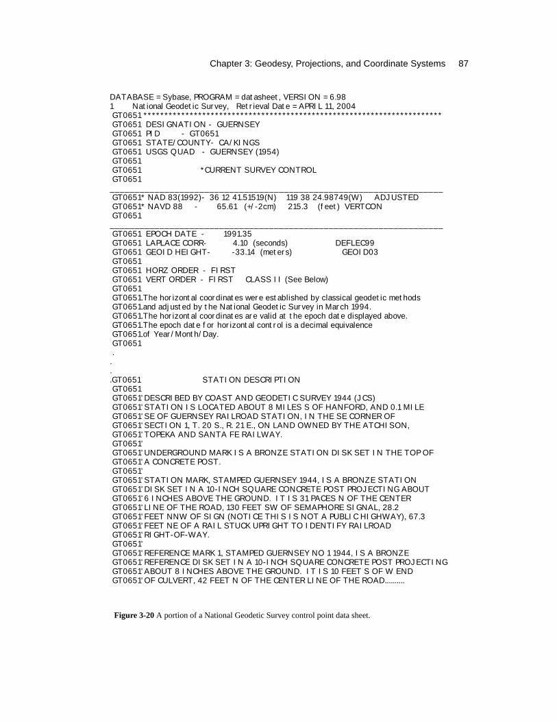
Figure 3-20 lists a partial description of a control point data sheet for a station named Guernsey, located in Kings County, Califor-nia. This station was first surveyed in 1944, and is a first-order horizontal and vertical control point. Only a portion of the four-page description is shown here. Datasheets for each point include the name, history, physical description, directions for location, coordinates, relevant datums, and adjust-ment history.
Lists of precisely surveyed points may also be obtained from state, county, city, or other surveyors, along with a physical description of the points and their location relative to nearby features. These control points may then be used as starting locations for local surveys to develop a denser net-work of control points, and as a basis for the development of spatial data.
Chapter 3: Geodesy, Projections, and Coordinate Systems 87
Figure 3-20 A portion of a National Geodetic Survey control point data sheet.
DATABASE = Sybase, PROGRAM = datasheet, VERSION = 6.981 National Geodetic Survey, Retrieval Date = APRIL 11, 2004 GT0651 *********************************************************************** GT0651 DESIGNATION - GUERNSEY GT0651 PID - GT0651 GT0651 STATE/COUNTY- CA/KINGS GT0651 USGS QUAD - GUERNSEY (1954) GT0651 GT0651 *CURRENT SURVEY CONTROL GT0651 ___________________________________________________________________ GT0651* NAD 83(1992)- 36 12 41.51519(N) 119 38 24.98749(W) ADJUSTED GT0651* NAVD 88 - 65.61 (+/-2cm) 215.3 (feet) VERTCON GT0651 ___________________________________________________________________ GT0651 EPOCH DATE - 1991.35 GT0651 LAPLACE CORR- 4.10 (seconds) DEFLEC99 GT0651 GEOID HEIGHT- -33.14 (meters) GEOID03 GT0651 GT0651 HORZ ORDER - FIRST GT0651 VERT ORDER - FIRST CLASS II (See Below) GT0651 GT0651.The horizontal coordinates were established by classical geodetic methods GT0651.and adjusted by the National Geodetic Survey in March 1994. GT0651.The horizontal coordinates are valid at the epoch date displayed above. GT0651.The epoch date for horizontal control is a decimal equivalence GT0651.of Year/Month/Day. GT0651 ....GT0651 STATION DESCRIPTION GT0651 GT0651'DESCRIBED BY COAST AND GEODETIC SURVEY 1944 (JCS) GT0651'STATION IS LOCATED ABOUT 8 MILES S OF HANFORD, AND 0.1 MILE GT0651'SE OF GUERNSEY RAILROAD STATION, IN THE SE CORNER OF GT0651'SECTION 1, T. 20 S., R. 21 E., ON LAND OWNED BY THE ATCHISON, GT0651'TOPEKA AND SANTA FE RAILWAY. GT0651' GT0651'UNDERGROUND MARK IS A BRONZE STATION DISK SET IN THE TOP OF GT0651'A CONCRETE POST. GT0651' GT0651'STATION MARK, STAMPED GUERNSEY 1944, IS A BRONZE STATION GT0651'DISK SET IN A 10-INCH SQUARE CONCRETE POST PROJECTING ABOUT GT0651'6 INCHES ABOVE THE GROUND. IT IS 31 PACES N OF THE CENTER GT0651'LINE OF THE ROAD, 130 FEET SW OF SEMAPHORE SIGNAL, 28.2 GT0651'FEET NNW OF SIGN (NOTICE THIS IS NOT A PUBLIC HIGHWAY), 67.3 GT0651'FEET NE OF A RAIL STUCK UPRIGHT TO IDENTIFY RAILROAD GT0651'RIGHT-OF-WAY. GT0651' GT0651'REFERENCE MARK 1, STAMPED GUERNSEY NO 1 1944, IS A BRONZE GT0651'REFERENCE DISK SET IN A 10-INCH SQUARE CONCRETE POST PROJECTING GT0651'ABOUT 8 INCHES ABOVE THE GROUND. IT IS 10 FEET S OF W END GT0651'OF CULVERT, 42 FEET N OF THE CENTER LINE OF THE ROAD..........
88 GIS Fundamentals
Map Projections and Coordinate SystemsDatums tell us the latitudes and longi-
tudes of a set of points on an ellipsoid. We need to transfer the locations of features measured with reference to these datum points from the curved ellipsoid to a flat map. A map projection is a systematic ren-dering of locations from the curved Earth surface onto a flat map surface. Points are “projected” from the Earth surface and onto the map surface.
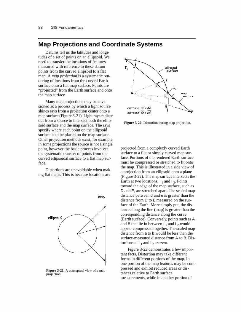
Many map projections may be envi-sioned as a process by which a light source shines rays from a projection center onto a map surface (Figure 3-21). Light rays radiate out from a source to intersect both the ellip-soid surface and the map surface. The rays specify where each point on the ellipsoid surface is to be placed on the map surface. Other projection methods exist, for example in some projections the source is not a single point, however the basic process involves the systematic transfer of points from the curved ellipsoidal surface to a flat map sur-face.
Distortions are unavoidable when mak-ing flat maps. This is because locations are
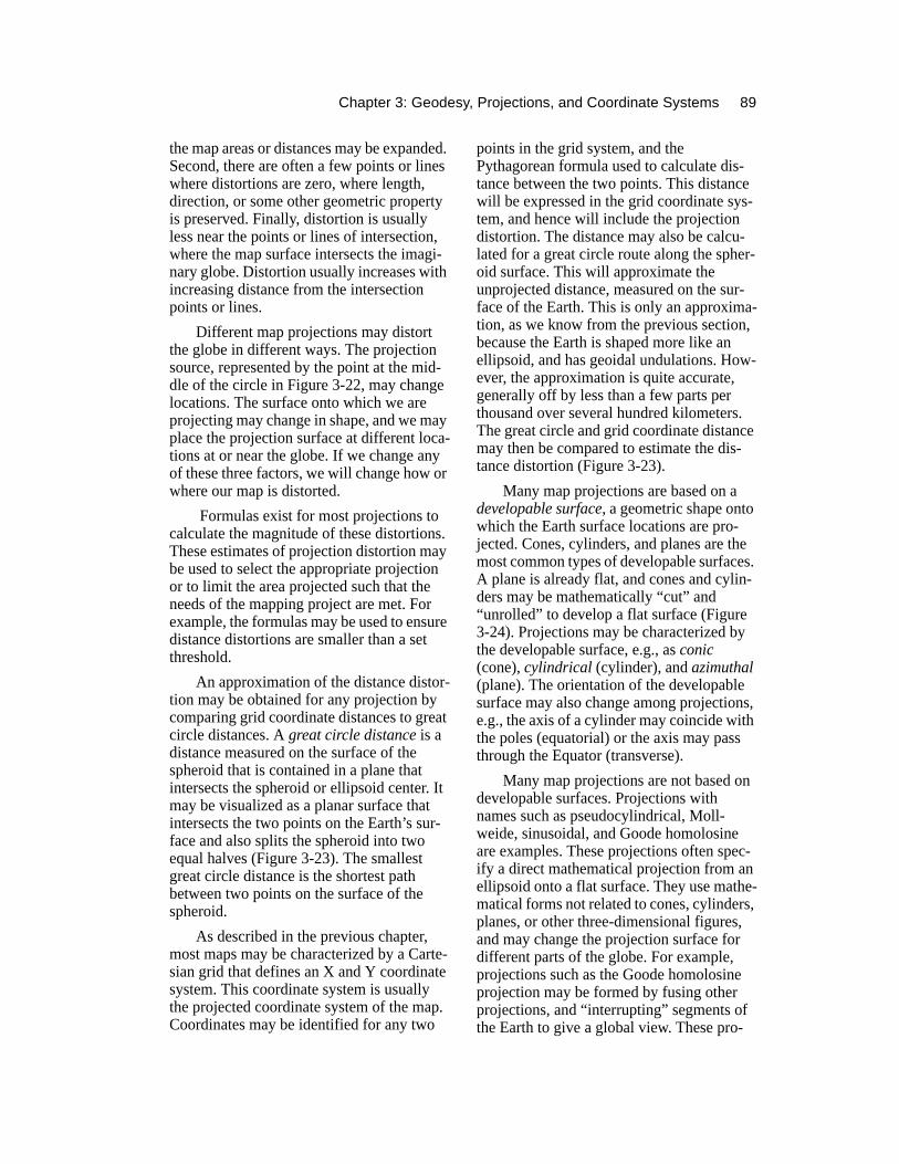
projected from a complexly curved Earth surface to a flat or simply curved map sur-face. Portions of the rendered Earth surface must be compressed or stretched to fit onto the map. This is illustrated in a side view of a projection from an ellipsoid onto a plane (Figure 3-22). The map surface intersects the Earth at two locations, I1 and I2. Points toward the edge of the map surface, such as D and E, are stretched apart. The scaled map distance between d and e is greater than the distance from D to E measured on the sur-face of the Earth. More simply put, the dis-tance along the line (map) is greater than the corresponding distance along the curve (Earth surface). Conversely, points such as A and B that lie in between I1 and I2 would appear compressed together. The scaled map distance from a to b would be less than the surface-measured distance from A to B. Dis-tortions at I1 and I2 are zero.
Figure 3-22 demonstrates a few impor-tant facts. Distortion may take different forms in different portions of the map. In one portion of the map features may be com-pressed and exhibit reduced areas or dis-tances relative to Earth surface measurements, while in another portion of
Figure 3-21: A conceptual view of a map projection.
Figure 3-22: Distortion during map projection.
Chapter 3: Geodesy, Projections, and Coordinate Systems 89
the map areas or distances may be expanded. Second, there are often a few points or lines where distortions are zero, where length, direction, or some other geometric property is preserved. Finally, distortion is usually less near the points or lines of intersection, where the map surface intersects the imagi-nary globe. Distortion usually increases with increasing distance from the intersection points or lines.
Different map projections may distort the globe in different ways. The projection source, represented by the point at the mid-dle of the circle in Figure 3-22, may change locations. The surface onto which we are projecting may change in shape, and we may place the projection surface at different loca-tions at or near the globe. If we change any of these three factors, we will change how or where our map is distorted.
Formulas exist for most projections to calculate the magnitude of these distortions. These estimates of projection distortion may be used to select the appropriate projection or to limit the area projected such that the needs of the mapping project are met. For example, the formulas may be used to ensure distance distortions are smaller than a set threshold.
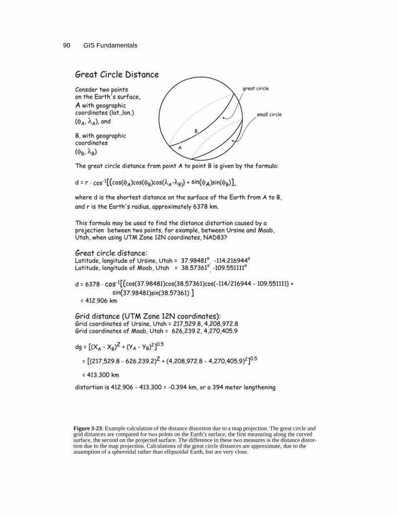
An approximation of the distance distor-tion may be obtained for any projection by comparing grid coordinate distances to great circle distances. A great circle distance is a distance measured on the surface of the spheroid that is contained in a plane that intersects the spheroid or ellipsoid center. It may be visualized as a planar surface that intersects the two points on the Earth’s sur-face and also splits the spheroid into two equal halves (Figure 3-23). The smallest great circle distance is the shortest path between two points on the surface of the spheroid.
As described in the previous chapter, most maps may be characterized by a Carte-sian grid that defines an X and Y coordinate system. This coordinate system is usually the projected coordinate system of the map. Coordinates may be identified for any two
points in the grid system, and the Pythagorean formula used to calculate dis-tance between the two points. This distance will be expressed in the grid coordinate sys-tem, and hence will include the projection distortion. The distance may also be calcu-lated for a great circle route along the spher-oid surface. This will approximate the unprojected distance, measured on the sur-face of the Earth. This is only an approxima-tion, as we know from the previous section, because the Earth is shaped more like an ellipsoid, and has geoidal undulations. How-ever, the approximation is quite accurate, generally off by less than a few parts per thousand over several hundred kilometers. The great circle and grid coordinate distance may then be compared to estimate the dis-tance distortion (Figure 3-23).
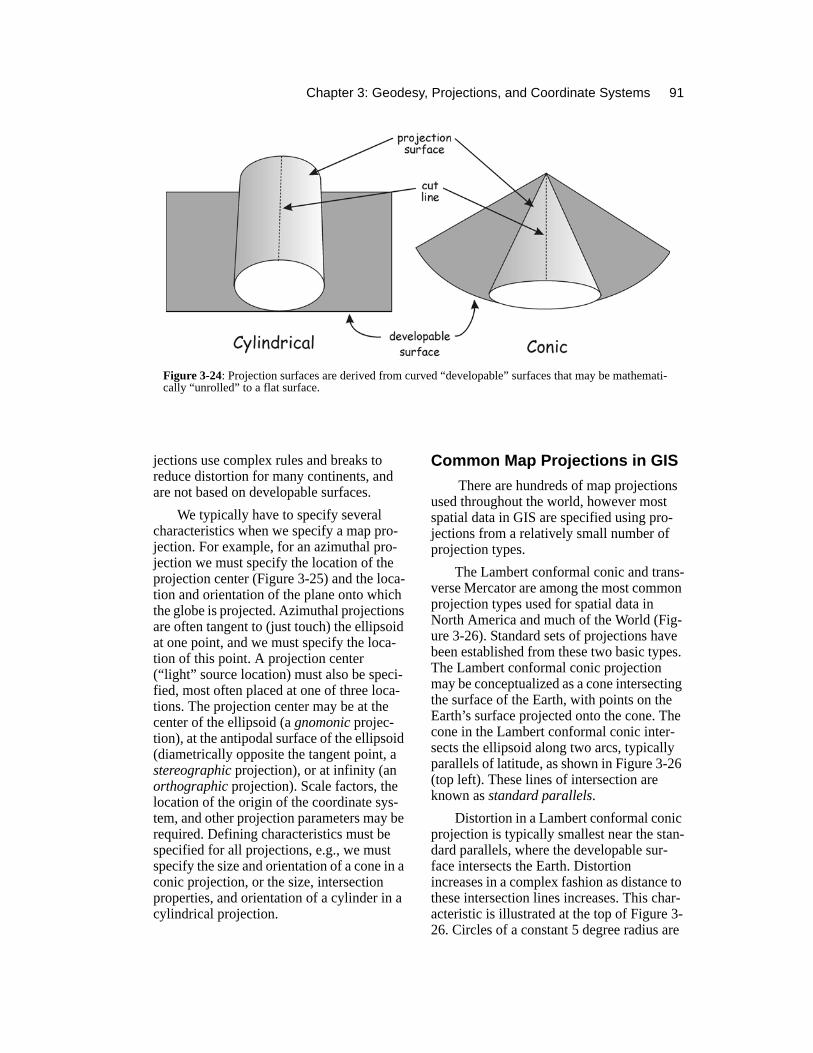
Many map projections are based on a developable surface, a geometric shape onto which the Earth surface locations are pro-jected. Cones, cylinders, and planes are the most common types of developable surfaces. A plane is already flat, and cones and cylin-ders may be mathematically “cut” and “unrolled” to develop a flat surface (Figure 3-24). Projections may be characterized by the developable surface, e.g., as conic (cone), cylindrical (cylinder), and azimuthal (plane). The orientation of the developable surface may also change among projections, e.g., the axis of a cylinder may coincide with the poles (equatorial) or the axis may pass through the Equator (transverse).
Many map projections are not based on developable surfaces. Projections with names such as pseudocylindrical, Moll-weide, sinusoidal, and Goode homolosine are examples. These projections often spec-ify a direct mathematical projection from an ellipsoid onto a flat surface. They use mathe-matical forms not related to cones, cylinders, planes, or other three-dimensional figures, and may change the projection surface for different parts of the globe. For example, projections such as the Goode homolosine projection may be formed by fusing other projections, and “interrupting” segments of the Earth to give a global view. These pro-
90 GIS Fundamentals
Figure 3-23: Example calculation of the distance distortion due to a map projection. The great circle and grid distances are compared for two points on the Earth’s surface, the first measuring along the curved surface, the second on the projected surface. The difference in these two measures is the distance distor-tion due to the map projection. Calculations of the great circle distances are approximate, due to the assumption of a spheroidal rather than ellipsoidal Earth, but are very close.
Chapter 3: Geodesy, Projections, and Coordinate Systems 91
jections use complex rules and breaks to reduce distortion for many continents, and are not based on developable surfaces.
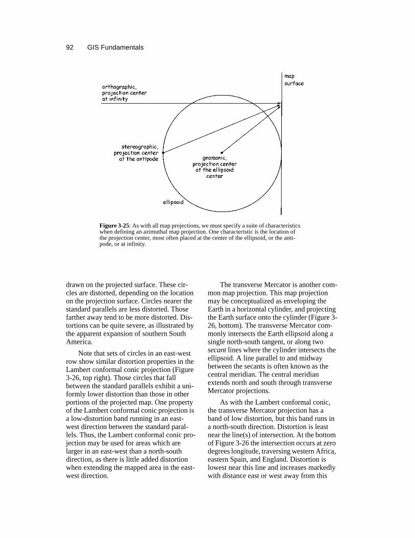
We typically have to specify several characteristics when we specify a map pro-jection. For example, for an azimuthal pro-jection we must specify the location of the projection center (Figure 3-25) and the loca-tion and orientation of the plane onto which the globe is projected. Azimuthal projections are often tangent to (just touch) the ellipsoid at one point, and we must specify the loca-tion of this point. A projection center (“light” source location) must also be speci-fied, most often placed at one of three loca-tions. The projection center may be at the center of the ellipsoid (a gnomonic projec-tion), at the antipodal surface of the ellipsoid (diametrically opposite the tangent point, a stereographic projection), or at infinity (an orthographic projection). Scale factors, the location of the origin of the coordinate sys-tem, and other projection parameters may be required. Defining characteristics must be specified for all projections, e.g., we must specify the size and orientation of a cone in a conic projection, or the size, intersection properties, and orientation of a cylinder in a cylindrical projection.
Common Map Projections in GIS There are hundreds of map projections
used throughout the world, however most spatial data in GIS are specified using pro-jections from a relatively small number of projection types.
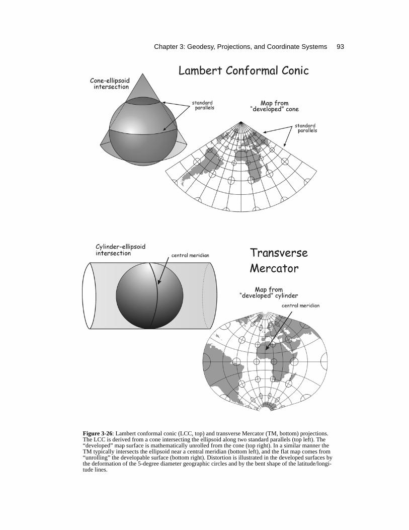
The Lambert conformal conic and trans-verse Mercator are among the most common projection types used for spatial data in North America and much of the World (Fig-ure 3-26). Standard sets of projections have been established from these two basic types. The Lambert conformal conic projection may be conceptualized as a cone intersecting the surface of the Earth, with points on the Earth’s surface projected onto the cone. The cone in the Lambert conformal conic inter-sects the ellipsoid along two arcs, typically parallels of latitude, as shown in Figure 3-26 (top left). These lines of intersection are known as standard parallels.
Distortion in a Lambert conformal conic projection is typically smallest near the stan-dard parallels, where the developable sur-face intersects the Earth. Distortion increases in a complex fashion as distance to these intersection lines increases. This char-acteristic is illustrated at the top of Figure 3-26. Circles of a constant 5 degree radius are
Figure 3-24: Projection surfaces are derived from curved “developable” surfaces that may be mathemati-cally “unrolled” to a flat surface.
92 GIS Fundamentals
drawn on the projected surface. These cir-cles are distorted, depending on the location on the projection surface. Circles nearer the standard parallels are less distorted. Those farther away tend to be more distorted. Dis-tortions can be quite severe, as illustrated by the apparent expansion of southern South America.
Note that sets of circles in an east-west row show similar distortion properties in the Lambert conformal conic projection (Figure 3-26, top right). Those circles that fall between the standard parallels exhibit a uni-formly lower distortion than those in other portions of the projected map. One property of the Lambert conformal conic projection is a low-distortion band running in an east-west direction between the standard paral-lels. Thus, the Lambert conformal conic pro-jection may be used for areas which are larger in an east-west than a north-south direction, as there is little added distortion when extending the mapped area in the east-west direction.
The transverse Mercator is another com-mon map projection. This map projection may be conceptualized as enveloping the Earth in a horizontal cylinder, and projecting the Earth surface onto the cylinder (Figure 3-26, bottom). The transverse Mercator com-monly intersects the Earth ellipsoid along a single north-south tangent, or along two secant lines where the cylinder intersects the ellipsoid. A line parallel to and midway between the secants is often known as the central meridian. The central meridian extends north and south through transverse Mercator projections.
As with the Lambert conformal conic, the transverse Mercator projection has a band of low distortion, but this band runs in a north-south direction. Distortion is least near the line(s) of intersection. At the bottom of Figure 3-26 the intersection occurs at zero degrees longitude, traversing western Africa, eastern Spain, and England. Distortion is lowest near this line and increases markedly with distance east or west away from this
Figure 3-25: As with all map projections, we must specify a suite of characteristics when defining an azimuthal map projection. One characteristic is the location of the projection center, most often placed at the center of the ellipsoid, or the anti-pode, or at infinity.
Chapter 3: Geodesy, Projections, and Coordinate Systems 93
Figure 3-26: Lambert conformal conic (LCC, top) and transverse Mercator (TM, bottom) projections. The LCC is derived from a cone intersecting the ellipsoid along two standard parallels (top left). The “developed” map surface is mathematically unrolled from the cone (top right). In a similar manner the TM typically intersects the ellipsoid near a central meridian (bottom left), and the flat map comes from “unrolling” the developable surface (bottom right). Distortion is illustrated in the developed surfaces by the deformation of the 5-degree diameter geographic circles and by the bent shape of the latitude/longi-tude lines.
94 GIS Fundamentals
line, e.g., the shape of South America is severely distorted in the bottom right of Fig-ure 3-26. For this reason transverse Mercator projections are often used for areas that extend in a north-south direction, as there is little added distortion extending in that direction.
Different projection parameters may be used to specify an appropriate coordinate system for a region of interest. Specific stan-dard parallels or central meridians are used to minimize distortion over a mapping area. An origin location, measurement units, x and y (or northing and easting) offsets, a scale factor, and other parameters may also be required to define a specific projection. Once a projection is defined then the coordi-nates of every point on the surface of the Earth may be determined, usually by a closed-form or approximate mathematical formula.
The State Plane Coordinate Sys-tem
The State Plane Coordinate System is a standard set of projections for the United States. The State Plane coordinate system specifies positions in a Cartesian coordinate system over several county to whole-state areas. There are typically one or more State Plane coordinate systems defined for each state in the United States. More than one State Plane zone may be required to limit distortion errors due to the map projection.
State Plane systems greatly facilitate surveying, mapping, and spatial data devel-opment in a GIS, particularly when county or larger areas are involved. Over relatively small areas the surface of the Earth can be assumed to be flat without introducing much distortion. However, Earth curvature causes area, distance, and shape distortion to increase when we assume a flat surface over larger areas. The State Plane system pro-vides a common coordinate reference for horizontal coordinates over large areas while limiting error to specified maximum values. Zones are specified in each state such that projection distortions are kept below one
part in 10,000. State Plane coordinate sys-tems are used in many types of work, includ-ing property surveys, property subdivisions, large-scale construction projects, and photo-grammetric mapping, and are often adopted for GIS.
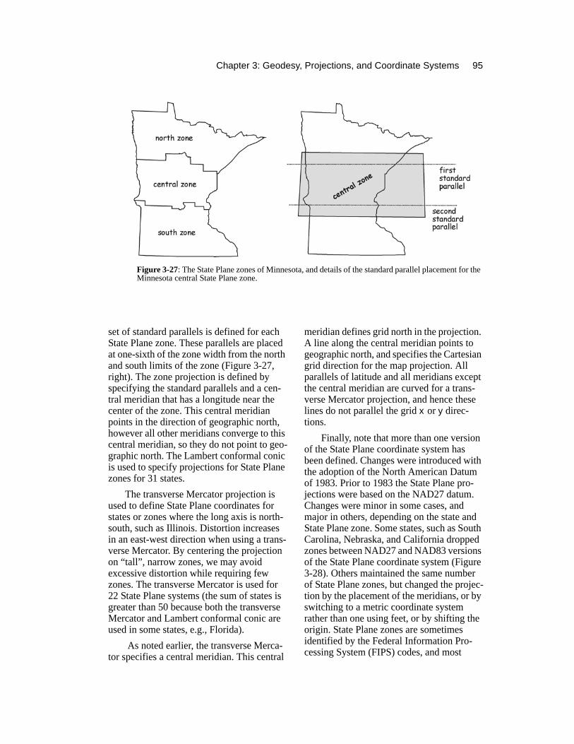
One State Plane projection zone may suffice for small states. Larger states com-monly require several zones, each with a dif-ferent projection, for each of several geographic zones of the state. For example Delaware has one State Plane coordinate zone, while California has 7, and Alaska has 10 State Plane coordinate zones, each corre-sponding to a different projection within the state. Zones are added to a state to ensure acceptable projection distortion within all zones (Figure 3-27, left). Within each zone, the distance on the curving Earth surface dif-fers by less than one part in 10,000 from the distance on the flat projection surface. Zones are defined by county, parish, or other municipal boundaries. For example, the Minnesota south/central zone boundary runs approximately east-west through the state along defined county boundaries (Figure 3-27, left).
The State Plane coordinate system is based on two basic types of map projections: the Lambert conformal conic and the trans-verse Mercator projections. Different projec-tions are used for each state or sub-area within a state, and are chosen to minimize distortion within a given state and zone. Because distortion in a transverse Mercator increases with distance from the central meridian, this projection type is most often used with states that have a long north-south axis (e.g., Illinois or New Hampshire). Con-versely, a Lambert conformal conic projec-tion is most often used when the long axis of a state is in the east-west direction (e.g. North Carolina and Virginia). When comput-ing the State Plane coordinates, points are projected from their geodetic latitudes and longitudes to x and y coordinates in the State Plane systems.
The Lambert conformal conic projection is specified in part by two standard parallels that run in an east-west direction. A different
Chapter 3: Geodesy, Projections, and Coordinate Systems 95
set of standard parallels is defined for each State Plane zone. These parallels are placed at one-sixth of the zone width from the north and south limits of the zone (Figure 3-27, right). The zone projection is defined by specifying the standard parallels and a cen-tral meridian that has a longitude near the center of the zone. This central meridian points in the direction of geographic north, however all other meridians converge to this central meridian, so they do not point to geo-graphic north. The Lambert conformal conic is used to specify projections for State Plane zones for 31 states.
The transverse Mercator projection is used to define State Plane coordinates for states or zones where the long axis is north-south, such as Illinois. Distortion increases in an east-west direction when using a trans-verse Mercator. By centering the projection on “tall”, narrow zones, we may avoid excessive distortion while requiring few zones. The transverse Mercator is used for 22 State Plane systems (the sum of states is greater than 50 because both the transverse Mercator and Lambert conformal conic are used in some states, e.g., Florida).
As noted earlier, the transverse Merca-tor specifies a central meridian. This central
meridian defines grid north in the projection. A line along the central meridian points to geographic north, and specifies the Cartesian grid direction for the map projection. All parallels of latitude and all meridians except the central meridian are curved for a trans-verse Mercator projection, and hence these lines do not parallel the grid x or y direc-tions.
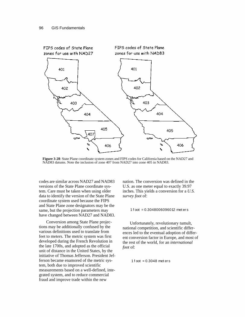
Finally, note that more than one version of the State Plane coordinate system has been defined. Changes were introduced with the adoption of the North American Datum of 1983. Prior to 1983 the State Plane pro-jections were based on the NAD27 datum. Changes were minor in some cases, and major in others, depending on the state and State Plane zone. Some states, such as South Carolina, Nebraska, and California dropped zones between NAD27 and NAD83 versions of the State Plane coordinate system (Figure 3-28). Others maintained the same number of State Plane zones, but changed the projec-tion by the placement of the meridians, or by switching to a metric coordinate system rather than one using feet, or by shifting the origin. State Plane zones are sometimes identified by the Federal Information Pro-cessing System (FIPS) codes, and most
Figure 3-27: The State Plane zones of Minnesota, and details of the standard parallel placement for the Minnesota central State Plane zone.
96 GIS Fundamentals
codes are similar across NAD27 and NAD83 versions of the State Plane coordinate sys-tem. Care must be taken when using older data to identify the version of the State Plane coordinate system used because the FIPS and State Plane zone designators may be the same, but the projection parameters may have changed between NAD27 and NAD83.
Conversion among State Plane projec-tions may be additionally confused by the various definitions used to translate from feet to meters. The metric system was first developed during the French Revolution in the late 1700s, and adopted as the official unit of distance in the United States, by the initiative of Thomas Jefferson. President Jef-ferson became enamored of the metric sys-tem, both due to improved scientific measurements based on a well-defined, inte-grated system, and to reduce commercial fraud and improve trade within the new
nation. The conversion was defined in the U.S. as one meter equal to exactly 39.97 inches. This yields a conversion for a U.S. survey foot of:
Unfortunately, revolutionary tumult, national competition, and scientific differ-ences led to the eventual adoption of differ-ent conversion factor in Europe, and most of the rest of the world, for an international foot of:
Figure 3-28: State Plane coordinate system zones and FIPS codes for California based on the NAD27 and NAD83 datums. Note the inclusion of zone 407 from NAD27 into zone 405 in NAD83.
1 foot = 0.3048006096012 meters
1 foot = 0.3048 meters
Chapter 3: Geodesy, Projections, and Coordinate Systems 97
The U.S. definition of a foot is slightly longer than the European definition, by about one part in five million. Both systems were used in measuring distance, the U.S. conversion of surveys in the U.S., and the international conversion of surveys or mea-surements elsewhere. The European conver-sion was adopted as the standard for all measures under an international agreement in the 1950s. However, there was a long his-tory of the use of the U.S. conversion in U.S. geodetic and land surveys. Therefore, the U.S. conversion was deemed the U.S. survey foot. This slightly longer metric to foot con-version factor should be used for all conver-sions among geodetic coordinate systems within the U.S., for example, when convert-ing from a State Plane coordinate system specified in feet to one specified in meters.
Universal Transverse Mercator Coordinate System
Another standard coordinate system has been based on the transverse Mercator pro-jection, distinct from the State Plane system. This system is known as the Universal
Transverse Mercator (UTM) coordinate sys-tem. The State Plane system is defined only for the United States. The UTM is a global coordinate system. It is widely used in the U.S.A. and other parts of North America, and is also used in many other countries worldwide.
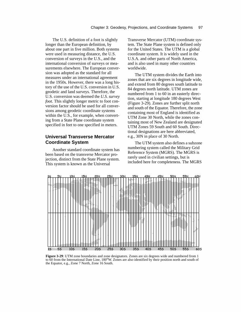
The UTM system divides the Earth into zones that are six degrees in longitude wide, and extend from 80 degrees south latitude to 84 degrees north latitude. UTM zones are numbered from 1 to 60 in an easterly direc-tion, starting at longitude 180 degrees West (Figure 3-29). Zones are further split north and south of the Equator. Therefore, the zone containing most of England is identified as UTM Zone 30 North, while the zones con-taining most of New Zealand are designated UTM Zones 59 South and 60 South. Direc-tional designations are here abbreviated, e.g., 30N in place of 30 North.
The UTM system also defines a subzone numbering system called the Military Grid Reference System (MGRS). The MGRS is rarely used in civilian settings, but is included here for completeness. The MGRS
Figure 3-29: UTM zone boundaries and zone designators. Zones are six degrees wide and numbered from 1 to 60 from the International Date Line, 180oW. Zones are also identified by their position north and south of the Equator, e.g., Zone 7 North, Zone 16 South.
98 GIS Fundamentals
subdivides each zone into subzones that span eight degrees of latitude. These subzones are designated by a letter. Subzone squares 100 km on a side are then designated with repeat-ing sequences. The MGRS combines the zone, subzone, and grid identifiers with coordinate numbers to identify locations on the Earth’s surface. The MGRS was never widely used outside of the military, where there was a strong need to rapidly and unam-biguously define location for continental to global military operations, and also provide some information on the precision of the coordinate measurement.
The UTM coordinate system is common for data and study areas spanning large regions, e.g., several State Plane zones. Many data from U.S. federal government sources are in a UTM coordinate system because many agencies manage land span-ning large areas, and the UTM is a well-
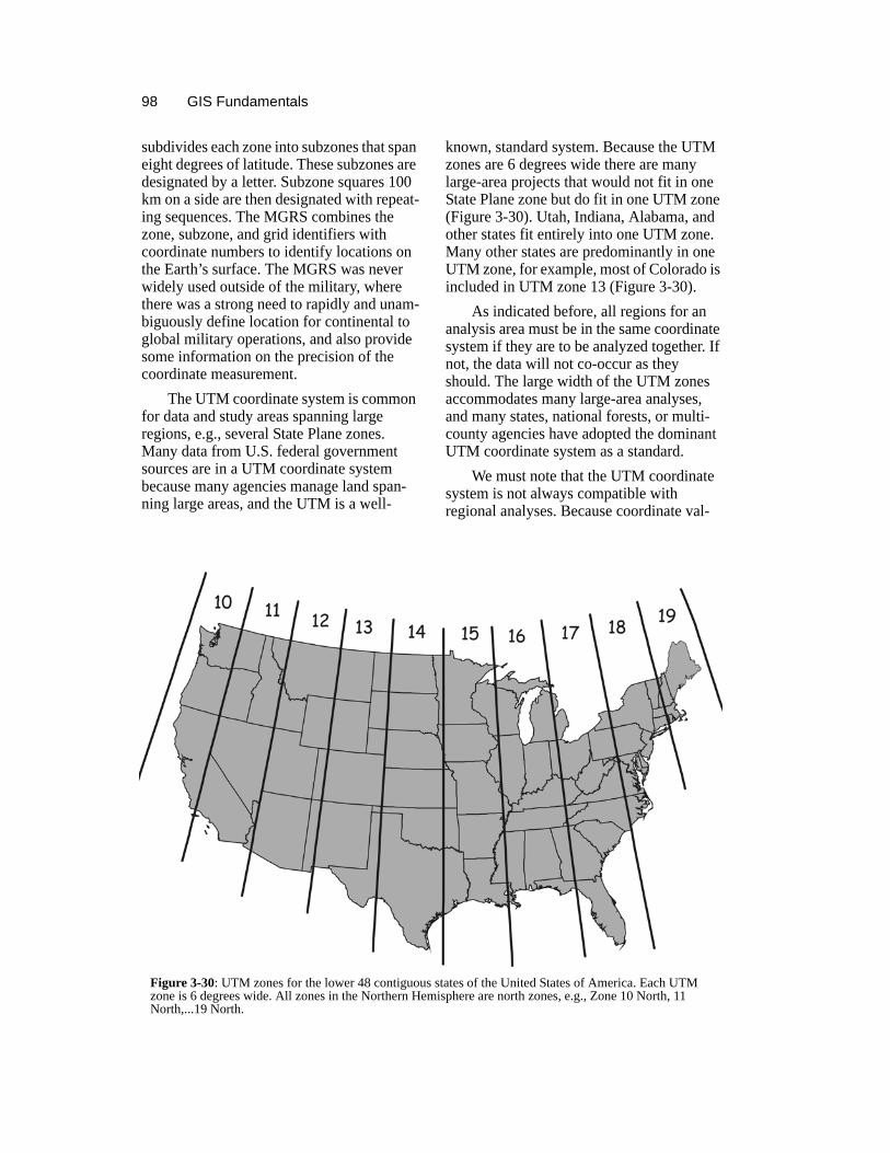
known, standard system. Because the UTM zones are 6 degrees wide there are many large-area projects that would not fit in one State Plane zone but do fit in one UTM zone (Figure 3-30). Utah, Indiana, Alabama, and other states fit entirely into one UTM zone. Many other states are predominantly in one UTM zone, for example, most of Colorado is included in UTM zone 13 (Figure 3-30).
As indicated before, all regions for an analysis area must be in the same coordinate system if they are to be analyzed together. If not, the data will not co-occur as they should. The large width of the UTM zones accommodates many large-area analyses, and many states, national forests, or multi-county agencies have adopted the dominant UTM coordinate system as a standard.
We must note that the UTM coordinate system is not always compatible with regional analyses. Because coordinate val-
Figure 3-30: UTM zones for the lower 48 contiguous states of the United States of America. Each UTM zone is 6 degrees wide. All zones in the Northern Hemisphere are north zones, e.g., Zone 10 North, 11 North,...19 North.
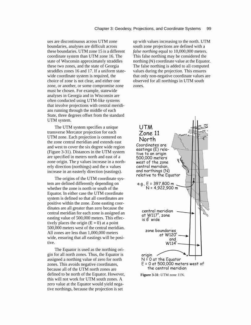
Chapter 3: Geodesy, Projections, and Coordinate Systems 99
ues are discontinuous across UTM zone boundaries, analyses are difficult across these boundaries. UTM zone 15 is a different coordinate system than UTM zone 16. The state of Wisconsin approximately straddles these two zones, and the state of Georgia straddles zones 16 and 17. If a uniform state-wide coordinate system is required, the choice of zone is not clear, and either one zone, or another, or some compromise zone must be chosen. For example, statewide analyses in Georgia and in Wisconsin are often conducted using UTM-like systems that involve projections with central meridi-ans running through the middle of each State, three degrees offset from the standard UTM system.
The UTM system specifies a unique transverse Mercator projection for each UTM zone. Each projection is centered on the zone central meridian and extends east and west to cover the six degree wide region (Figure 3-31). Distances in the UTM system are specified in meters north and east of a zone origin. The y values increase in a north-erly direction (northings) and the x values increase in an easterly direction (eastings).
The origins of the UTM coordinate sys-tem are defined differently depending on whether the zone is north or south of the Equator. In either case the UTM coordinate system is defined so that all coordinates are positive within the zone. Zone easting coor-dinates are all greater than zero because the central meridian for each zone is assigned an easting value of 500,000 meters. This effec-tively places the origin (E = 0) at a point 500,000 meters west of the central meridian. All zones are less than 1,000,000 meters wide, ensuring that all eastings will be posi-tive.
The Equator is used as the northing ori-gin for all north zones. Thus, the Equator is assigned a northing value of zero for north zones. This avoids negative coordinates, because all of the UTM north zones are defined to be north of the Equator. However, this will not work for UTM south zones. A zero value at the Equator would yield nega-tive northings, because the projection is set
up with values increasing to the north. UTM south zone projections are defined with a false northing equal to 10,000,000 meters. This false northing may be considered the northing (N) coordinate value at the Equator. The false northing is added to all computed values during the projection. This ensures that only non-negative coordinate values are observed for all northings in UTM south zones.
Figure 3-31: UTM zone 11N.
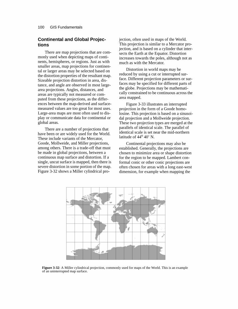
100 GIS Fundamentals
Continental and Global Projec-tions
There are map projections that are com-monly used when depicting maps of conti-nents, hemispheres, or regions. Just as with smaller areas, map projections for continen-tal or larger areas may be selected based on the distortion properties of the resultant map. Sizeable projection distortion in area, dis-tance, and angle are observed in most large-area projections. Angles, distances, and areas are typically not measured or com-puted from these projections, as the differ-ences between the map-derived and surface-measured values are too great for most uses. Large-area maps are most often used to dis-play or communicate data for continental or global areas.
There are a number of projections that have been or are widely used for the World. These include variants of the Mercator, Goode, Mollweide, and Miller projections, among others. There is a trade-off that must be made in global projections, between a continuous map surface and distortion. If a single, uncut surface is mapped, then there is severe distortion in some portion of the map. Figure 3-32 shows a Miller cylindrical pro-
jection, often used in maps of the World. This projection is similar to a Mercator pro-jection, and is based on a cylinder that inter-sects the Earth at the Equator. Distortion increases towards the poles, although not as much as with the Mercator.
Distortion in world maps may be reduced by using a cut or interrupted sur-face. Different projection parameters or sur-faces may be specified for different parts of the globe. Projections may be mathemati-cally constrained to be continuous across the area mapped.
Figure 3-33 illustrates an interrupted projection in the form of a Goode homo-losine. This projection is based on a sinusoi-dal projection and a Mollweide projection. These two projection types are merged at the parallels of identical scale. The parallel of identical scale is set near the mid-northern latitude of 44o 40’ N.
Continental projections may also be established. Generally, the projections are chosen to minimize area or shape distortion for the region to be mapped. Lambert con-formal conic or other conic projections are often chosen for areas with a long east-west dimension, for example when mapping the
Figure 3-32: A Miller cylindrical projection, commonly used for maps of the World. This is an example of an uninterrupted map surface.
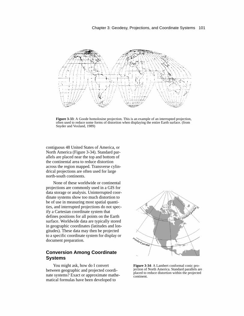
Chapter 3: Geodesy, Projections, and Coordinate Systems 101
contiguous 48 United States of America, or North America (Figure 3-34). Standard par-allels are placed near the top and bottom of the continental area to reduce distortion across the region mapped. Transverse cylin-drical projections are often used for large north-south continents.
None of these worldwide or continental projections are commonly used in a GIS for data storage or analysis. Uninterrupted coor-dinate systems show too much distortion to be of use in measuring most spatial quanti-ties, and interrupted projections do not spec-ify a Cartesian coordinate system that defines positions for all points on the Earth surface. Worldwide data are typically stored in geographic coordinates (latitudes and lon-gitudes). These data may then be projected to a specific coordinate system for display or document preparation.
Conversion Among Coordinate Systems
You might ask, how do I convert between geographic and projected coordi-nate systems? Exact or approximate mathe-matical formulas have been developed to
Figure 3-33: A Goode homolosine projection. This is an example of an interrupted projection, often used to reduce some forms of distortion when displaying the entire Earth surface. (from Snyder and Voxland, 1989)
Figure 3-34: A Lambert conformal conic pro-jection of North America. Standard parallels are placed to reduce distortion within the projected continent.
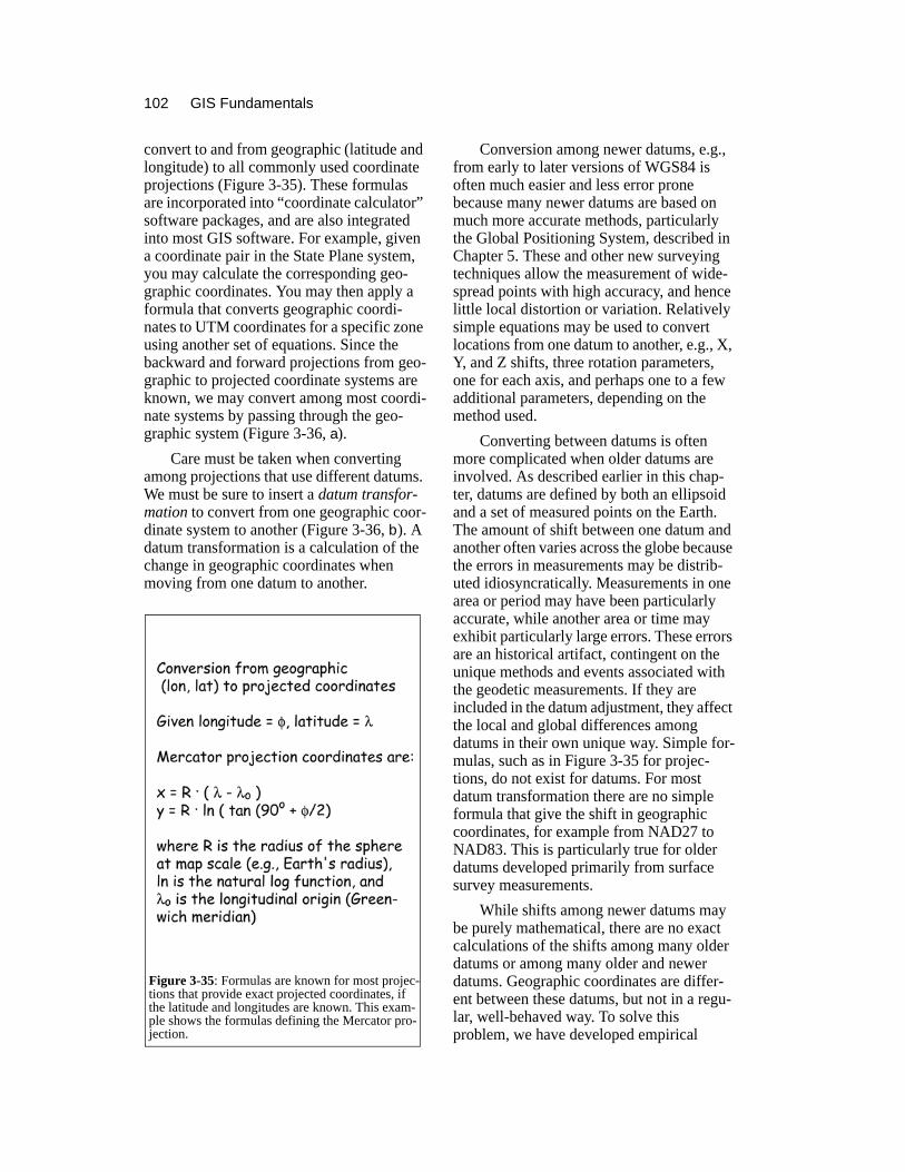
102 GIS Fundamentals
convert to and from geographic (latitude and longitude) to all commonly used coordinate projections (Figure 3-35). These formulas are incorporated into “coordinate calculator” software packages, and are also integrated into most GIS software. For example, given a coordinate pair in the State Plane system, you may calculate the corresponding geo-graphic coordinates. You may then apply a formula that converts geographic coordi-nates to UTM coordinates for a specific zone using another set of equations. Since the backward and forward projections from geo-graphic to projected coordinate systems are known, we may convert among most coordi-nate systems by passing through the geo-graphic system (Figure 3-36, a).
Care must be taken when converting among projections that use different datums. We must be sure to insert a datum transfor-mation to convert from one geographic coor-dinate system to another (Figure 3-36, b). A datum transformation is a calculation of the change in geographic coordinates when moving from one datum to another.
Conversion among newer datums, e.g., from early to later versions of WGS84 is often much easier and less error prone because many newer datums are based on much more accurate methods, particularly the Global Positioning System, described in Chapter 5. These and other new surveying techniques allow the measurement of wide-spread points with high accuracy, and hence little local distortion or variation. Relatively simple equations may be used to convert locations from one datum to another, e.g., X, Y, and Z shifts, three rotation parameters, one for each axis, and perhaps one to a few additional parameters, depending on the method used.
Converting between datums is often more complicated when older datums are involved. As described earlier in this chap-ter, datums are defined by both an ellipsoid and a set of measured points on the Earth. The amount of shift between one datum and another often varies across the globe because the errors in measurements may be distrib-uted idiosyncratically. Measurements in one area or period may have been particularly accurate, while another area or time may exhibit particularly large errors. These errors are an historical artifact, contingent on the unique methods and events associated with the geodetic measurements. If they are included in the datum adjustment, they affect the local and global differences among datums in their own unique way. Simple for-mulas, such as in Figure 3-35 for projec-tions, do not exist for datums. For most datum transformation there are no simple formula that give the shift in geographic coordinates, for example from NAD27 to NAD83. This is particularly true for older datums developed primarily from surface survey measurements.
While shifts among newer datums may be purely mathematical, there are no exact calculations of the shifts among many older datums or among many older and newer datums. Geographic coordinates are differ-ent between these datums, but not in a regu-lar, well-behaved way. To solve this problem, we have developed empirical
Figure 3-35: Formulas are known for most projec-tions that provide exact projected coordinates, if the latitude and longitudes are known. This exam-ple shows the formulas defining the Mercator pro-jection.
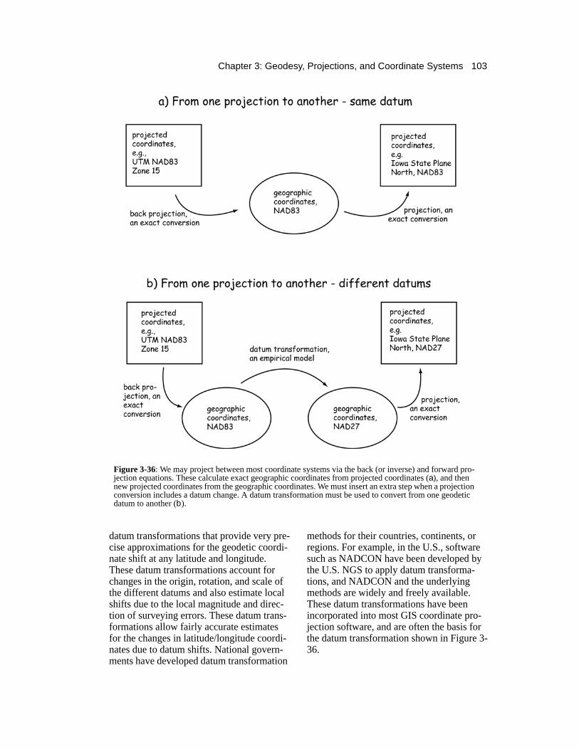
Chapter 3: Geodesy, Projections, and Coordinate Systems 103
datum transformations that provide very pre-cise approximations for the geodetic coordi-nate shift at any latitude and longitude. These datum transformations account for changes in the origin, rotation, and scale of the different datums and also estimate local shifts due to the local magnitude and direc-tion of surveying errors. These datum trans-formations allow fairly accurate estimates for the changes in latitude/longitude coordi-nates due to datum shifts. National govern-ments have developed datum transformation
methods for their countries, continents, or regions. For example, in the U.S., software such as NADCON have been developed by the U.S. NGS to apply datum transforma-tions, and NADCON and the underlying methods are widely and freely available. These datum transformations have been incorporated into most GIS coordinate pro-jection software, and are often the basis for the datum transformation shown in Figure 3-36.
Figure 3-36: We may project between most coordinate systems via the back (or inverse) and forward pro-jection equations. These calculate exact geographic coordinates from projected coordinates (a), and then new projected coordinates from the geographic coordinates. We must insert an extra step when a projection conversion includes a datum change. A datum transformation must be used to convert from one geodetic datum to another (b).
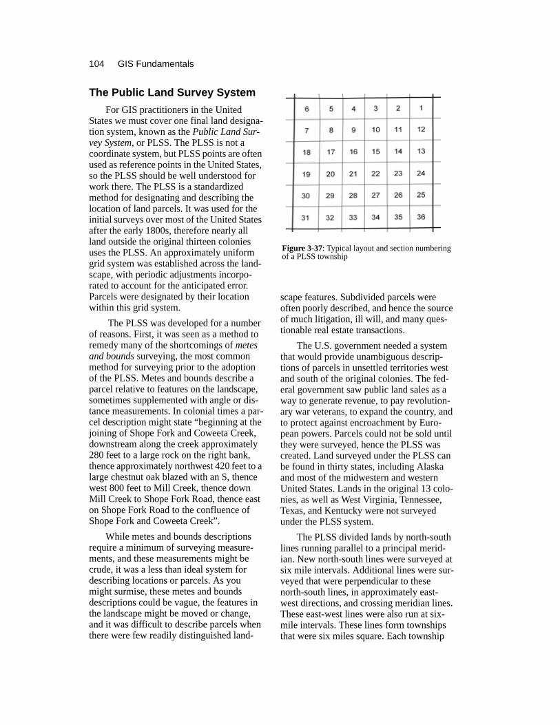
104 GIS Fundamentals
The Public Land Survey SystemFor GIS practitioners in the United
States we must cover one final land designa-tion system, known as the Public Land Sur-vey System, or PLSS. The PLSS is not a coordinate system, but PLSS points are often used as reference points in the United States, so the PLSS should be well understood for work there. The PLSS is a standardized method for designating and describing the location of land parcels. It was used for the initial surveys over most of the United States after the early 1800s, therefore nearly all land outside the original thirteen colonies uses the PLSS. An approximately uniform grid system was established across the land-scape, with periodic adjustments incorpo-rated to account for the anticipated error. Parcels were designated by their location within this grid system.
The PLSS was developed for a number of reasons. First, it was seen as a method to remedy many of the shortcomings of metes and bounds surveying, the most common method for surveying prior to the adoption of the PLSS. Metes and bounds describe a parcel relative to features on the landscape, sometimes supplemented with angle or dis-tance measurements. In colonial times a par-cel description might state “beginning at the joining of Shope Fork and Coweeta Creek, downstream along the creek approximately 280 feet to a large rock on the right bank, thence approximately northwest 420 feet to a large chestnut oak blazed with an S, thence west 800 feet to Mill Creek, thence down Mill Creek to Shope Fork Road, thence east on Shope Fork Road to the confluence of Shope Fork and Coweeta Creek”.
While metes and bounds descriptions require a minimum of surveying measure-ments, and these measurements might be crude, it was a less than ideal system for describing locations or parcels. As you might surmise, these metes and bounds descriptions could be vague, the features in the landscape might be moved or change, and it was difficult to describe parcels when there were few readily distinguished land-
scape features. Subdivided parcels were often poorly described, and hence the source of much litigation, ill will, and many ques-tionable real estate transactions.
The U.S. government needed a system that would provide unambiguous descrip-tions of parcels in unsettled territories west and south of the original colonies. The fed-eral government saw public land sales as a way to generate revenue, to pay revolution-ary war veterans, to expand the country, and to protect against encroachment by Euro-pean powers. Parcels could not be sold until they were surveyed, hence the PLSS was created. Land surveyed under the PLSS can be found in thirty states, including Alaska and most of the midwestern and western United States. Lands in the original 13 colo-nies, as well as West Virginia, Tennessee, Texas, and Kentucky were not surveyed under the PLSS system.
The PLSS divided lands by north-south lines running parallel to a principal merid-ian. New north-south lines were surveyed at six mile intervals. Additional lines were sur-veyed that were perpendicular to these north-south lines, in approximately east-west directions, and crossing meridian lines. These east-west lines were also run at six-mile intervals. These lines form townships that were six miles square. Each township
Figure 3-37: Typical layout and section numbering of a PLSS township
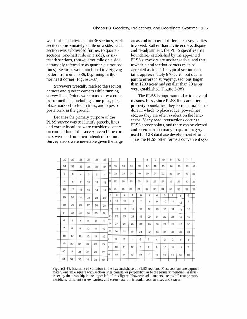
Chapter 3: Geodesy, Projections, and Coordinate Systems 105
was further subdivided into 36 sections, each section approximately a mile on a side. Each section was subdivided further, to quarter-sections (one-half mile on a side), or six-teenth sections, (one-quarter mile on a side, commonly referred to as quarter-quarter sec-tions). Sections were numbered in a zig-zag pattern from one to 36, beginning in the northeast corner (Figure 3-37).
Surveyors typically marked the section corners and quarter-corners while running survey lines. Points were marked by a num-ber of methods, including stone piles, pits, blaze marks chiseled in trees, and pipes or posts sunk in the ground.
Because the primary purpose of the PLSS survey was to identify parcels, lines and corner locations were considered static on completion of the survey, even if the cor-ners were far from their intended location. Survey errors were inevitable given the large
areas and number of different survey parties involved. Rather than invite endless dispute and re-adjustment, the PLSS specifies that boundaries established by the appointed PLSS surveyors are unchangeable, and that township and section corners must be accepted as true. The typical section con-tains approximately 640 acres, but due in part to errors in surveying, sections larger than 1200 acres and smaller than 20 acres were established (Figure 3-38).
The PLSS is important today for several reasons. First, since PLSS lines are often property boundaries, they form natural corri-dors in which to place roads, powerlines, etc., so they are often evident on the land-scape. Many road intersections occur at PLSS corner points, and these can be viewed and referenced on many maps or imagery used for GIS database development efforts. Thus the PLSS often forms a convenient sys-
Figure 3-38: Example of variation in the size and shape of PLSS sections. Most sections are approxi-mately one mile square with section lines parallel or perpendicular to the primary meridian, as illus-trated by the township in the upper left of this figure. However, adjustments due to different primary meridians, different survey parties, and errors result in irregular section sizes and shapes.
106 GIS Fundamentals
tem to co-register GIS data layers. PLSS corners and lines are often plotted on gov-ernment maps (e.g. 1:24,000 quads) or avail-able as digital data (e.g. National Cartographic Information Center Digital Line Graphs). Further, PLSS corners are sometimes re-surveyed using high precision methods to provide cadastral control, partic-ularly when a GIS is to be developed. Thus these points may be useful to register spatial data layers to the Earth's surface.
SummaryIn order to enter coordinates in a GIS,
we need to uniquely define the location of all points on Earth. We must develop a refer-ence frame for our coordinate system, and locate positions on this system. Since the Earth is a curved surface and we work with flat maps, we must somehow reconcile these two views of the World. We define positions on the globe via geodesy and surveying. We convert these locations to flat surfaces via map projections.
We begin by modeling the Earth’s shape with an ellipsoid. An ellipsoid differs from the geoid, a gravitationally-defined Earth surface, and these differences caused some early confusion in the adoption of standard global ellipsoids. There is a long history of ellipsoidal measurement, and we have arrived at our best estimates of global and regional ellipsoids after collecting large, painstakingly-developed sets of precise sur-face and astronomical measurements. These measurements are combined into datums, and these datums are used to specify the coordinate locations of points on the surface of the Earth.
Map projections are a systematic render-ing of points from the curved Earth surface onto a flat map surface. While there are many purely mathematical or purely empiri-cal map projections, the most common map projections used in GIS are based on devel-opable surfaces. Cones, cylinders, and planes are the most common developable surfaces. A map projection is constructed by passing rays from a projection center
through both the Earth surface and the devel-opable surface. Points on the Earth are pro-jected along the rays and onto the developable surface. This surface is then mathematically unrolled to form a flat map.
Standard sets of projections are com-monly used for spatial data in a GIS. In the United States, the UTM and State Plane coordinate systems define a standard set of map projections that are widely used. Other map projections are commonly used for con-tinental or global maps, and for smaller maps in other regions of the World.
A datum transformation is often required when performing map projections. This accounts for differences in geographic coordinates due to changes in the shape or origin of the spheroid, and in some cases to datum adjustments. Models may be analyti-cal or empirical, and are often applied as a step in the map projection process when input and output projection datums differ.
A system of land division was estab-lished in the United States known as the Public Land Survey System (PLSS). This is not a coordinate system but rather a method for unambiguously and systematically defin-ing parcels of land based on regularly spaced survey lines in approximately north-south and east-west directions. Intersection coordi-nates have been precisely measured for many of these survey lines, and are often used as a reference grid for further surveys or land subdivision.
Chapter 3: Geodesy, Projections, and Coordinate Systems 107
Suggested Reading
Bossler, J.D., Datums and geodetic systems, in Manual of Geospatial Technology, J. Bossler, Ed., Taylor and Francis, London, 2002.
Brandenburger, A. J. and Gosh, S. K., The world’s topographic and cadastral mapping opera-tions, Photogrammetric Engineering and Remote Sensing, 1985, 51:437-444.
Burkholder, E.F., Computation of horizontal/level distances, Journal of Surveying Engineer-ing, 1993, 117:104-119.
Colvocoresses, A.P., The gridded map, Photogrammetric Engineering and Remote Sensing, 1997, 63:371-376.
Doyle, F.J., Map conversion and the UTM Grid, Photogrammetric Engineering and Remote Sensing, 1997 63:367-370.
Habib, A., Coordinate transformation, in Manual of Geospatial Technology, J. Bossler, Ed., Taylor and Francis, London, 2002.
Iliffe, J. C., Datums and Map Projections for Remote Sensing, GIS, and Surveying, CRC Press, Boca Raton, 2000.
Keay, J., The Great Arc, Harper Collins, London, 2000.
Leick, A., Accuracy standards for modern three-dimensional geodetic networks, Surveying and Land Information Systems 53:111-127, 1993.
Maling, D. H., Coordinate Systems and Map Projections, George Phillip, London, 1992.
Schwartz, C.R., North American Datum of 1983, NOAA Professional Paper NOS 2, National Geodetic Survey, Rockville, 1989.
Smith, J., Introduction to Geodesy: The History and Concepts of Modern Geodesy, Wiley, New York, 1997.
Sobel, D., Longitude, Penguin Books, New York, 1995.
Snyder, J., Flattening the Earth: Two Thousand Years of Map Projections, University of Chi-cago Press, Chicago, 1993.
Snyder, J. P., Map Projections, A Working Manual, USGS Professional Paper No. 1396, United States Government Printing Office, Washington D.C., 1987.
Snyder, J.P., and Voxland, P.M., An Album of Map Projections, USGS Professional Paper No. 1453, United States Government Printing Office, Washington D.C., 1989.
108 GIS Fundamentals
Tobler, W.R., A classification of map projections, Annals of the Association of American Geographers, 1962, 52:167-175.
Welch, R., and Homsey, Datum shifts for UTM coordinates, Photogrammetric Engineering and Remote Sensing, 1997, 63:371-376.
Wolf, P. R., and C.D. Ghilani, Elementary Surveying, 10th Ed., Prentice-Hall, Upper Saddle River, New Jersey, 2002.
Zilkoski, D., J. Richards, and G. Young, Results of the general adjustment of the North Amer-ican Vertical Datum of 1988, Surveying and Land Information Systems, 1992, 53:133-149
Chapter 3: Geodesy, Projections, and Coordinate Systems 109
Study Questions
Can you describe how Eratosthenes estimated the circumference of the Earth? What value did he obtain?
How did the method of Eratosthenes and Posidonius differ? Were their estimates sim-ilar, and how accurate were their estimates relative to current measurements?
What is an ellipsoid? How does an ellipse differ from a sphere? What is the equation for the flattening factor?
Why do different ellipsoids have different radii? Can you provide three reasons?
Can you define the geoid? How does it differ from the ellipsoid, or the surface of the Earth? How do we measure the position of the geoid?
Can you define a parallel or meridian in a geographic coordinate system? Where do the “horizontal” and “vertical” zero lines occur?
How does magnetic north differ from the geographic North Pole?
Can you define a datum? Can you describe how datums are developed?
Why are there multiple datums, even for the same place on Earth? Can you define what we mean when we say there is a datum shift?
What is a triangulation survey, a Bilby tower, and a benchmark?
What is a map projection? Can you define a gnomonic, stereographic, or ortho-graphic projection?
What is a developable surface? What are the most common shapes for a developable surface?
Can you describe the State Plane coordinate system? What type of projections are used in a State Plane coordinate system?
Can you define and describe the Universal Transverse Mercator coordinate system? What type of developable surface is used with a UTM projection? What are UTM zones, where is the origin of a zone, and how are negative coordinates avoided?
What is a datum transformation? How does it differ from a map projection?
Can you describe the Public Land Survey System? Is it a coordinate system? What is its main purpose?

110 GIS Fundamentals