3 Exponential and Logarithmic Functions · Graphs of Logarithmic Functions The parent logarithmic...
35
Copyright © Cengage Learning. All rights reserved. 3 Exponential and Logarithmic Functions
Transcript of 3 Exponential and Logarithmic Functions · Graphs of Logarithmic Functions The parent logarithmic...

Copyright © Cengage Learning. All rights reserved.
3 Exponential and Logarithmic
Functions

Copyright © Cengage Learning. All rights reserved.
3.2 Logarithmic Functions
and Their Graphs

3
What You Should Learn
• Recognize and evaluate logarithmic functions
with base a.
• Graph logarithmic functions with base a.
• Recognize, evaluate, and graph natural
logarithmic functions.
• Use logarithmic functions to model and solve
real-life problems.

4
Logarithmic Functions

5
Logarithmic Functions
When a function is one-to-one—that is, when the function
has the property that no horizontal line intersects its graph
more than once—the function must have an inverse
function. Every function of the form
f (x) = ax, where a > 0 and a 1,
passes the Horizontal Line Test and therefore must have
an inverse function. This inverse function is called the
logarithmic function with base a.

6
Logarithmic Functions

7
Logarithmic Functions
Every logarithmic equation can be written in an equivalent
exponential form and every exponential equation can be
written in logarithmic form.
So, the equations
y = logax and x = ay
are equivalent.
8
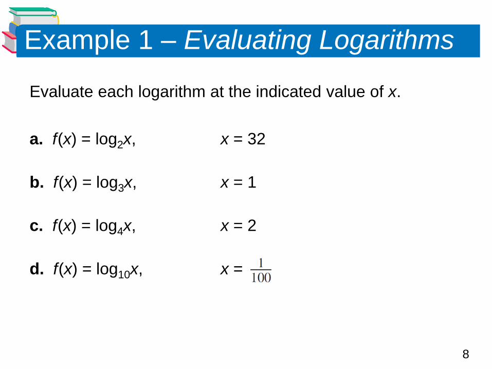
Example 1 – Evaluating Logarithms
Evaluate each logarithm at the indicated value of x.
a. f (x) = log2x, x = 32
b. f (x) = log3x, x = 1
c. f (x) = log4x, x = 2
d. f (x) = log10x, x =

9
Example 1 – Solution
a. f (32) = log232 = 5 because 25 = 32.
b. f (1) = log31 = 0 because 30 = 1.
c. f (2) = log42 = because 41/2 = = 2.
d. f ( ) = log10 = –2 because 10–2 = = .

10
Logarithmic Functions
The logarithmic function with base 10 is called the
common logarithmic function.
The properties of logarithms listed below follow directly
from the definition of the logarithmic function with base a.

11
Example 3 – Using Properties of Logarithms
a. Solve for x: log2x = log23
b. Solve for x: log44 = x
c. Simplify: log55x
d. Simplify: 7log714
Solution:
a. Using the One-to-One Property (Property 4), you can
conclude that x = 3.

12
Example 3 – Solution
b. Using Property 2, you can conclude that x = 1.
c. Using the Inverse Property (Property 3), it follows that
log55x = x.
d. Using the Inverse Property (Property 3), it follows that
7
log 714 = 14.
cont’d
13
Graphs of Logarithmic Functions

14
Graphs of Logarithmic Functions
To sketch the graph of y = loga x, you can use the fact that
the graphs of inverse functions are reflections of each other
in the line y = x.

15
Example 4 – Graphs of Exponential and Logarithmic Functions
In the same coordinate plane, sketch the graph of each
function by hand.
a. f (x) = 2x
b. g (x) = log2x
Solution:
a. For f (x) = 2x, construct a table of values.

16
Example 4 – Solution
By plotting these points
and Connecting them with a
smooth curve, you obtain the
graph of f shown in Figure 3.12.
b. Because g (x) = log2 x is the inverse function of f (x) = 2x,
the graph of g is obtained by plotting the points (f (x), x)
and connecting them with a smooth curve.
The graph of g is a reflection of the graph of f in the line
y = x, as shown in Figure 3.12.
cont’d
Figure 3.12

17
Graphs of Logarithmic Functions
The parent logarithmic function
f (x) = logax, a > 0, a 1
is the inverse function of the exponential function. Its
domain is the set of positive real numbers and its range is
the set of all real numbers. This is the opposite of the
exponential function.
Moreover, the logarithmic function has the y-axis as a
vertical asymptote, whereas the exponential function has
the x-axis as a horizontal asymptote.

18
Graphs of Logarithmic Functions
Many real-life phenomena with slow rates of growth can be
modeled by logarithmic functions. The basic characteristics
of the logarithmic function are summarized below
Graph of f (x) = loga x, a > 1
Domain: (0, )
Range: ( )
Intercept: (1, 0)
Increasing on: (0, )
y-axis is a vertical asymptote (loga x → as x → 0+)

19
Graphs of Logarithmic Functions
Continuous Reflection of graph of f (x)= ax in the line y = x

20
Example 6 – Library of Parent function f (x) = loga x
Each of the following functions is a transformation of the
graph of
f (x) = log10x.
a. Because g (x) = log10(x – 1) = f (x – 1), the graph of g can
be obtained by shifting the graph of f one unit to the
right, as shown in Figure 3.14.
Figure 3.14
21
Example 6 – Library of Parent function f (x) = loga x
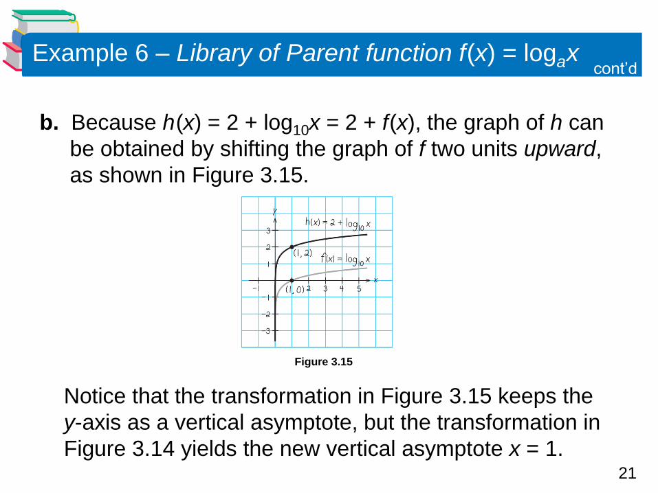
b. Because h (x) = 2 + log10x = 2 + f (x), the graph of h can
be obtained by shifting the graph of f two units upward,
as shown in Figure 3.15.
Notice that the transformation in Figure 3.15 keeps the
y-axis as a vertical asymptote, but the transformation in
Figure 3.14 yields the new vertical asymptote x = 1.
Figure 3.15
cont’d

22
The Natural Logarithmic Function

23
The Natural Logarithmic Function
The function f (x) = ex is one-to-one and so has an inverse
function. This inverse function is called the natural
logarithmic function and is denoted by the special symbol
In x, read as “the natural log of x” or “el en of x.”

24
The Natural Logarithmic Function
The equations y = ln x and x = ey are equivalent. Note that
the natural logarithm ln x is written without a base.
The base is understood to be e.

25
Example 7 – Evaluating the Natural Logarithmic function
Use a calculator to evaluate the function
f (x) = ln x
at each indicated value of x.
a. x = 2
b. x = 0.3
c. x = –1
d. x = 1 +

26
Example 7 – Solution

27
The Natural Logarithmic Function
The following properties of logarithms are valid for natural
logarithms.

28
Example 8 – Using Properties of Natural Algorithms
Use the properties of natural logarithms to rewrite each
expression.
a. b. e ln 5 c. 4 ln 1 d. 2 ln e
Solution:
a. = ln e–1 = –1
b. e ln 5 = 5
c. 4 ln 1 = 4(0) = 0
d. 2 ln e = 2(1) = 2
Inverse Property
Inverse Property
Property 1
Property 2

29
Example 9 – Finding the Domains of Logarithmic Functions
Find the domain of each function.
a. f (x) = ln( x – 2) b. g (x) = ln(2 – x) c. h (x) = ln x2
Solution:
a. Because ln( x – 2) is defined only when
x – 2 > 0
it follows that the domain of f is (2, ).

30
Example 9 – Solution
b. Because ln (2 – x) is defined only when
2 – x > 0
it follows that the domain of g is ( , 2).
c. Because In x2 is defined only when
x2 > 0
it follows that the domain of h is all real numbers except
x = 0.
cont’d

31
Application

32
Example 10 – Psychology
Students participating in a psychology experiment attended
several lectures on a subject and were given an exam.
Every month for a year after the exam, the students were
retested to see how much of the material they
remembered. The average scores for the group are given
by the human memory model
f (t) = 75 – 6 ln(t + 1), 0 t 12
where t is the time in months.
The graph of f is shown in
Figure 3.17.
Figure 3.17

33
Example 10 – Psychology
a. What was the average score on the original exam (t = 0)?
b. What was the average score at the end of t = 2 months?
c. What was the average score at the end of t = 6 months?
Solution:
a. The original average score was
f (0) = 75 – 6 ln(0 + 1)
= 75 – 6 ln 1
= 75 – 6(0)
= 75.
cont’d

34
Example 10 – Solution
b. After 2 months, the average score was
f (2) = 75 – 6 ln(2 + 1)
= 75 – 6 ln 3
75 – 6(1.0986)
68.41.
cont’d

35
Example 10 – Solution
c. After 6 months, the average score was
f (6) = 75 – 6 ln(6 + 1)
= 75 – 6 ln 7
75 – 6(1.9459)
63.32.
cont’d