3 Experimental Method and Equipment

16

3 Experimental Method and

Equipment

3.1 Method and Principle

The following sections outline the fundamental ideas and perspectives of photoemission from

a highly volatile surface, which at first sight would seem incompatible with such a ultra-

high vacuum (UHV) electron spectroscopy method. It will be described in detail how a

liquid microjet can be constructed, and why the small dimensions together with a suitable

streaming velocity allow to measure electron binding energies and electron yields from liquids

despite their high vapor pressure. Finally, some basic aspects of photoemission will be

presented followed by a short review of the principle properties of synchrotron radiation

with emphasize on undulator radiation.

3.1.1 Matching Highly Volatile Surfaces with UHV Electron Spec-

troscopy

The main obstacle in applying a surface sensitive method, such as electron spectroscopy, to

studying processes at liquid interfaces is the principle difficulty to handle a liquid system

under vacuum conditions, and to detect photoelectrons originating from the liquid sample.

This explains today’s still very limited availability of photoemission data from liquids at high

pressures in general. The majority of common liquids and solutions are volatile, i.e. they

easily evaporate. Therefore, the main problem connected with electron spectroscopy on liquid

matter is the vapor pressure, which for typical laboratory solvents may be up to several

hundred mbar. This value is substantially higher than the maximum allowable pressure

inside an electron energy analyzer. Furthermore, as the liquid surface is covered by dense

vapor due to evaporation it is generally impossible to directly assess surface properties by the

3.1 Method and Principle 17

experiment. In photoelectron spectroscopy (PES; see section 3.1.3) one has to prevent sample

vapor molecules from colliding with the photoelectrons originating from the sample, here the

liquid jet, as they are heading for the electron energy analyzer. Note that even if the vapor

pressure of a liquid is sufficiently low to avoid collisions in the electron analyzer, the vapor

pressure directly above the liquid surface is generally so high that the liquid photoemission

spectrum would be entirely masked by that of the vapor. Besides the problem of high vapor

pressure of the liquid, which makes it impossible to obtain the required vacuum without

either freezing the sample itself or having it consumed by evaporation, one other problem is

to maintain a clean surface despite aging processes.

The earliest report on a vacuum surface study of a liquid dates back to an electron diffrac-

tion experiment by Wierl in 1930. For grazing incidence he observed electron diffraction rings

on a mercury surface which was steadily renewed by overflowing liquid [18]. However, this

rudimentary study was not considered particularly successful at that time. Microscopic liq-

uid structure studies by X-ray diffraction were also performed [19], but the results could

not be explained satisfactorily. This became possible only later, based on radial distribution

functions for intra- and intermolecular pairwise distances [20]. In the early studies of liquid

surfaces by means of photoelectron spectroscopy, the liquid was picked up by a rotating tar-

get, often a disk (stainless steel [21] or quartz [22]) partially immersed in a liquid reservoir.

The rotating wheel drags along a liquid film which can be scraped by a sapphire plate, thus

producing a thin liquid layer [23]. In this way a fresh surface of defined liquid layer thickness

was obtained and used for molecular beam scattering studies of surface corrugation. In 1981,

using monochromatized photons up to 12 eV, the photoelectron threshold energy of liquid

water of 10.06 eV was reported for conductor-supported liquids [22]. In another experiment,

a liquid film sample was created by a conically shaped metal trundle immersed in the liquid

and being rotated about its axis. This arrangement was used for electron spectroscopy for

chemical analysis (ESCA) measurements [24, 25] in 1986, however, a large amount of salt

had to be added in order to appreciably reduce the vapor pressure [25]. Another variant of

generating a liquid film on a substrate surface is the wetted metal wire which serves to con-

tinuously transport liquid into the observation region and to minimize the vapor load to the

vacuum chamber [24]. In the latter case, the temperature of the liquid was reduced by liquid

nitrogen, which lowered the vapor pressure considerably. Generally, previously unaccessi-

ble liquids of sufficiently low vapor pressure, ca. 10−2 mbar (or respectively low temperature

within their liquid range), such as glycol, methanol, toluene, formamide and others, could

be investigated. Charging of the low conductive liquid by the electron emission process was

18 3 Experimental Method and Equipment

minimized by restricting to very thin films on a metallic substrate. A detailed description

of the early liquid surface measurements is given in Ref. [4]. These methods could not be

applied to water, though. Similarly, optical absorption measurements in the VUV and XUV

spectral range are almost non-existent since again high vacuum is a prerequisite.

Hence, some other experimental technique was required!

3.1.2 Liquid Jet: Formation, Theory and Characteristics

One important empirical conclusion of the experiments mentioned above was that the prod-

uct of the vapor pressure p0 and the transfer length d required for transferring photoelectrons

to the spectrometer entrance has to be smaller than a characteristic value. For ultraviolet

photoelectron spectroscopy (UPS), with photoelectron energies on the order of some tens of

eV, the criterion p · d < 0.1Torr·mm (0.13mbar·mm) was reported [24]. For volatile liquids,

pure water for instance, this requirement can only be fulfilled if a very small surface area of

liquid is exposed to the vacuum. One has to imagine a liquid point source, so small, that the

number of vapor molecules quickly decreases (for short distances) to a sufficiently low value

that both photoelectrons directly emerging from the liquid sample pass the vapor without

collisions, and that at larger distance these electrons would reach the electron spectrometer.

The solution to that idea was to use a micro-sized liquid jet [26]. This method not only

matches high vacuum requirements, but it also provides continuous surface renewal due to

the suitably large velocity. Technically, a laminar jet is formed by forcing the liquid through

a small pinhole into an evacuated chamber [26]. If the jet diameter is sufficiently small that

the Knudsen condition [27] is fulfilled,

djet < λmol , (3.1)

a free vacuum surface of a volatile liquid may be achieved. Here, djet is the jet diameter and

λmol denotes the mean free path of the molecules at the corresponding thermal equilibrium.

From kinetic gas theory λmol of water molecules at a vapor pressure of 6.13mbar (4.6Torr)

is estimated to be on the order of 10µm [26]. The small size of the thin and continuous

liquid flow (liquid beam) combined with the low background pressure (∼ 10−5 mbar for water,

maintained by heavy pumping) results in nearly collision-free evaporation. Note that the

jet indeed guarantees a clean liquid beam surface even in the pressure range of 10−5 mbar,

because the surface is renewed all the time by its flow. Furthermore the continuous supply of

warmer water from the reservoir prevents the beam from freezing as a result of evaporative

cooling.


flight time [msec]

inte

nsity

[arb

. uni

ts]

0 1.0 2.0 3.00

0.5

1.0

10 µm

50 µm

Figure 3.1: Time-of-flight spectra of water molecules evaporating from the water jet [28]. For10 µm jet diameter a Maxwellian distribution is obtained implying collision-less evaporation.For 50 µm jet diameter water-water collisions lead to a modified Maxwellian distribution. Theformer is given by f(v) = Av2exp[−m(v−u)2/kBT ], where a flow velocity u is superimposedon the thermal velocity distribution; v is the molecular velocity. Here T denotes the localsurface temperature, m is the particle’s mass, kB is the Boltzmann constant, and A is a fitparameter. The fit in the figure, for the 10µm jet, corresponds to u = 0, and the obtainedsurface temperature is 281 K.

In order to directly prove collision-free evaporation under the experimental conditions,

measurements of the velocity distribution of the evaporated molecules at some distance

from the jet had been performed as reported in an earlier work by Faubel [28]. Typical

time-of-flight spectra of H2O molecules are presented in the Fig. 3.1 showing a Maxwellian

distribution for a 10µm jet, but a narrow supersonic velocity distribution for a 50µm jet.

The spectra thus confirm the expected transition from the collision to the collision-less regime

once the ratio between jet diameter and mean free path approaches the Knudsen limit [28].

Fitting the time-of-flight spectra obtained for the 10µm case by a standard Maxwellian

velocity distribution function provides a direct measure of the instantaneous local surface

temperature of the liquid for the actual vacuum evaporation conditions [28]. In this way a

value of 281K was obtained.

Jet instabilities and decay. The thin and continuous water beam is generated by

forcing the liquid water (pressurized by 80 bar He) through two sequential (platinum-iridium)

pinholes of 200 and 10µm diameter into the main vacuum chamber. The ideal, nonviscous

flow velocity for a thin wall diaphragm is related to the nozzle backing pressure p0 and the


liquid density ρ by the relation:

v =

√2p0

ρ, (3.2)

obtained by equating p0V with the kinetic energy mv2/2. For water with ρ ' 1000 kg/m3

at 4 C, the jet velocity is about 127m/s. Directly after the liquid jet emerges from the high

pressure behind the nozzle, it forms a straight, laminar flowing, cylindrical filament only

within the first 3 - 5mm. Very near the nozzle exit, the surface contracts (due to surface

tension) within a distance of a few nozzle diameters to its final diameter d (see Fig. 3.2).

For a nozzle with 10µm diameter a contraction factor of 0.63 was found by laser diffraction

measurements of the liquid jet diameter [29]. For larger distances (> 3 - 5mm) the jet decays

into droplets. According to Rayleigh [30], the decay is driven by capillary forces which tend

to reduce the energy of a long filament by breaking up the jet into a stream of droplets [4].

Using potential flow theory, it was shown that small spontaneous fluctuations of the jet radius

grow exponentially near a critical axial wavelength λc and lead to a radial modulation of the

jet resulting in its decay into droplets. For practically important cases the wavelength for

spontaneous jet decay is [4]:

λc ' 4.5djet , (3.3)

and the jet decay length L is given by the equation [4]

L = vt ' 3v

√ρd3

jet

σtens

, (3.4)

where ρ is the density of the liquid and σtens the surface tension. Rayleigh theory has been

later extended to viscous fluids by Weber [31], in which case the decay wavelength was found

to increase as follows

λc = πdjet

√2 + 6KOhn . (3.5)

Here KOhn is known as Ohnesorge number which provides an universal scaling number for

characterizing jet breakup regions and flow domains [32]:

KOhn =ηd√

ρσtensdjet

. (3.6)

Here ηd denotes the dynamical viscosity. For values KOhn 1 the jet flow is non-viscous.

Water jets are typical examples for this flow domain.

For a 6µm water jet (which is the actual jet diameter in the present experiments; see

above 3.2.1), assuming ρ ' 1000 kg/m3 for the water density, σtens = 0.073N/m for the

surface tension, and a value of ηd = 1mPa·s for the dynamical viscosity, one obtains λc =


cylindrical laminar flow sectionλc

L

djet dN

jet contraction

Figure 3.2: Schematic of the liquid jet decay into droplets at distance L from the nozzle.The decay is driven by capillary forces leading to spontaneous amplification of surface wavesat a critical wavelength λc.

32µm using equations 3.5 and 3.6. Then, with equation 3.4 the length L of the intact laminar

jet is calculated to be 3.5µm. This is in agreement with laser diffraction measurements from

the jet, which were performed at different distances from the 10µm nozzle.

Further details as to the role of surface tension and the decay mechanism of a liquid jet,

can be found in the pioneering work by Faubel [4].

3.1.3 Fundamental Aspects of Photoemission

The electronic structure of matter is one key information for understanding the respective

chemical and physical properties. A well established and widely used experimental technique

to access this information is photoelectron spectroscopy (PES), a technique based on the

photoelectric effect [33]. The subjects of PES are atoms or molecules in the gas phase,

solids, and, with special technical requirements, liquids. The outstanding feature of PES is

to single out individual electronic states by measuring photoelectron kinetic energies.

One simple approach in describing the photoemission process is the so-called three-step

model which considers the photoemission as being separable into three distinct and indepen-

dent processes [35]. At first, the photon is locally absorbed and an electron is excited. In the

second step the electron travels through the sample to the surface, and in the last step the

electron escapes through the surface into the vacuum where it is detected. This separation is

somewhat artificial and, in principle, the whole process of photoexcitation should be treated

as a single step.

By absorbing a photon of energy hν a system containing N electrons and being described

by an initial wave function ψi(N) and energy Ei(N), will be excited into a final state with


E = 0

kinetic energy of photoelectrons, Ekin

binding energy EB = hν - Ekin

nucleus

inner levels

valence bandhν

hνhν

Figure 3.3: Illustration of photoelectron spectroscopy [34]. The dashed lines represent theorbitals of the electrons. The binding energy of the photoelectrons is the difference betweenthe energy of the excitation photons and the kinetic energy of the electrons.

ψf (N − 1, k) and Ef (N − 1, k) and a photoelectron with kinetic energy Ekin will be emitted.

Energy conservation gives:

Ei(N) + hν = Ef (N − 1, k) + Ekin (3.7)

and thus the binding energy relative to the vacuum level may be defined as

EB(k) = Ef (N − 1, k)− Ei(N) , (3.8)

where the final state wave function ψf (N − 1, k) represents an atom with a hole in the level

k. If one assumes that no rearrangement of the electrons - either within the atom from which

the photoelectron originated or in the neighboring atoms - occurs following the ejection of

the photoelectron, then the remaining electrons after an ionization event are described by

the same wave function as in the initial state. Within the Hartree-Fock approximation this

leads to Koopmans’ theorem whereby the ionization energy is obtained directly from the

calculation of the neutral ground state [36] and is simply the negative of the atomic orbital

energy εk [37]:

EB(k) = −εk . (3.9)

This approximation is not entirely correct because after ejection of the electron from a

particular orbital k, the system will try to readjust its remaining N − 1 charges in such a

way as to minimize its energy (relaxation). Therefore, the correct binding energy is given by


the difference between the Koopmans’ binding energy −εk and a positive relaxation energy

Er:

EB(k) = −εk − Er . (3.10)

Relaxation is thus a final state effect. The assumption that the time needed for the removal

of one of the photoelectrons is much shorter than the time required for the rearrangement

of the valence electron charge distribution is referred to as the sudden approximation.

The time scale for the photoemission event depends on the velocity of the escaping pho-

toelectron and thus the sudden limit corresponds to high excitation energies. It is, however,

difficult to formulate strict criteria [38] for the applicability of the sudden approximation,

and the energy range within it is valid is still an open question.

At the other limit, known as the adiabatic excitation limit the photoelectron leaves the

atom slowly, in such a way that the electrons on or near the excited atom will lower their

energy by slowly adjusting to the new hole potential in an instantaneous, self-consistent

way [39]. This approximation corresponds to low excitation energies.

As previously described, the photoemission process involves the excitation of one electron

from an initial state (an atomic orbital) to a final state. The intensity of the photoemission

peak (photocurrent) depends on both the initial and final state wavefunctions ψi, ψf and of

the incident electromagnetic field ~E. Describing the system’s ground state by the Hamilto-

nian H0 and the ionizing photon beam as a small perturbation H′, the transition probability

per unit time between the two states is given by Fermi’s Golden Rule:

w =2π

~| < ψf |H

′|ψi > |2 δ(Ef − Ei − ~ω) . (3.11)

In the dipole approximation the perturbation can be written as:

H′= −~µ · ~E , (3.12)

where ~µ is the dipole moment and ~E is the external electric field.

PES is an extremely surface sensitive technique due to the strong interaction of the

electrons with matter. An electron travelling through a solid will have a certain inelastic

mean free path, i.e. a characteristic length that it can travel on the way out of the solid

without suffering an energy loss. This length, referred to as electron mean free path, strongly

depends on the electron kinetic energy. This relation is known as the universal mean free

path curve which is shown in Fig. 3.4. The minimum of this curve, in the ca. 20 - 120 eV

range is the region of maximum surface sensitivity (lowest escape depth).


1 10 100 1000

1000

100

10

1

kinetic energy [eV]

mea

n fr

ee p

ath

[mon

olay

ers]

Figure 3.4: Mean free path of electrons in solids as a function of their kinetic energy [40].

Since PES requires an incident photon of a known energy value, collimated monochro-

matic (single frequency) photons are desired. When photons in the ultraviolet (UV) spectral

region are used, the technique is called UV Photoelectron Spectroscopy (UPS), with X-ray

radiation one refers to XPS or ESCA (Electron Spectroscopy for Chemical Analysis). Using

tunable synchrotron radiation one may cover the whole spectral range from the near-UV to

the far X-ray regime.

The angular distribution anisotropy parameter β. In the dipole approximation

the differential cross section dσ/dΩ for photoionization of a randomly oriented sample by

linearly polarized light is defined by [41,42]

dσ(hν)

dΩ(Θ) =

σi(hν)

4π[1 + β(hν)P2(cosΘ)] . (3.13)

Here σi is the partial photoionization cross section, β is the asymmetry parameter, P2 is the

2nd order Legendre-Polynom (P2(cosΘ) = (3cos2Θ− 1)/2), and Θ is the angle between the

momentum vector of the ejected electron and the polarization vector of the incident photon.

The parameter β depends on the photon energy and on the nature of the molecular orbital

which is ionized. Possible values for β range between -1 and +2, otherwise the differential

cross section in equation 3.13 would become negative.

Knowledge of β is crucial for the proper interpretation of all experimental measurements

of photoionization process, unless the measurements are carried out at the magic angle, ΘM


β = 1.5

β = 0

β = -1β = 2

β = 1

Θ = 90

Θ = 0

E

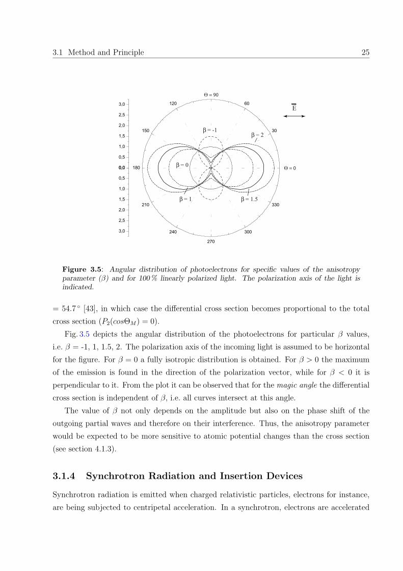
Figure 3.5: Angular distribution of photoelectrons for specific values of the anisotropyparameter (β) and for 100 % linearly polarized light. The polarization axis of the light isindicated.

= 54.7 [43], in which case the differential cross section becomes proportional to the total

cross section (P2(cosΘM) = 0).

Fig. 3.5 depicts the angular distribution of the photoelectrons for particular β values,

i.e. β = -1, 1, 1.5, 2. The polarization axis of the incoming light is assumed to be horizontal

for the figure. For β = 0 a fully isotropic distribution is obtained. For β > 0 the maximum

of the emission is found in the direction of the polarization vector, while for β < 0 it is

perpendicular to it. From the plot it can be observed that for the magic angle the differential

cross section is independent of β, i.e. all curves intersect at this angle.

The value of β not only depends on the amplitude but also on the phase shift of the

outgoing partial waves and therefore on their interference. Thus, the anisotropy parameter

would be expected to be more sensitive to atomic potential changes than the cross section

(see section 4.1.3).

3.1.4 Synchrotron Radiation and Insertion Devices

Synchrotron radiation is emitted when charged relativistic particles, electrons for instance,

are being subjected to centripetal acceleration. In a synchrotron, electrons are accelerated


and confined to nearly circular trajectories by magnetic fields. Due to the relativistic ve-

locities of the circulating electrons, the radiation emission pattern is enhanced into forward

direction within a narrow cone, tangentially to the orbit of the electrons. This is explained

in terms of a Lorentz transformation of the emission pattern from the particle’s coordinate

system to the laboratory frame. The natural collimation is one of the important properties

of synchrotron radiation. The opening angle of the cone (angular spread) is approximately

1/γ [43], with:

γ =E

m0c2, (3.14)

where E is the energy, m0 the mass of circulating electrons and c the velocity of light

(γ = 1/√

1− (v/c)2 is the electron’s Lorentz factor; v is the velocity of electrons). The

higher the kinetic energy of the charged particles the narrower the emission cone becomes,

and the spectrum of the emitted radiation extends to higher energies.

Due to its properties synchrotron radiation is by far superior to conventional light sources

such as X-ray tubes or discharge lamps. Synchrotron radiation not only allows for a wide

energy range (from IR to hard X-ray), but also for high flux, small spot size and a high degree

of polarization. Yet, other techniques, such as laser plasmas or high harmonic generation

from gas jets, for instance, may be advantageous for some applications.

Typically, the spectral intensity of synchrotron radiation is characterized by its brilliance

[43] which is defined as:

B =(spectral flux into 0.1 % bandwith)

source area (mm2) · solid angle (mrad2) · 100(mA). (3.15)

Brilliance is thus proportional to the number of photons normalized by the source area,

horizontal and vertical divergences at 100mA ring current.

Generation of synchrotron radiation requires the coordination of several systems: (i) the

electron production stage, (ii) a primary accelerating system for the electron beam, and

(iii) a storage ring to store the electrons for several hours. Finally, one needs (iv) outlet

(front-end) systems to guide the photon beam to the experiment. This is achieved with

vacuum tubes (beamlines) either following a bending magnet or an insertion device (IDs,

see below). Optical elements direct the light to a monochromator, which selects the desired

photon energy.

As the experiments presented were performed at the electron storage ring BESSY II in

Berlin, some features of this facility will be described below. Electrons emitted by a cathode

are accelerated to an energy of 100 keV. The second stage is a microtron, the central part


of which is a linear accelerator with a strong high frequency electrical field (3GHz). As a

consequence, the circulating electrons are bunched and they will achieve at this point an

energy of 50MeV. From the microtron electrons are transferred into the vacuum chamber

of the synchrotron (booster) where they are further accelerated to a final energy of 1.7GeV.

As the electron energy increase would lead to a larger trajectory, magnetic field corrections

are necessary to keep the particles on the same orbit. From this synchronization of field and

energy, the name synchrotron evolved. Finally, the electrons are injected through a transfer

channel into the storage ring.

The storage ring is an accelerator designed to keep the electrons in a closed orbit at

relativistic but constant velocity. BESSY’s storage ring has a circumference of 240m con-

taining 16 straight sections. Each straight section is followed by bending magnets deflecting

the electron beam into the next section. The circulating electrons have transverse motions

with respect to the ideal path, which cannot be compensated for by the dipole magnets only.

Hence, in order to keep the electrons within the closed orbit, additional focusing magnets,

such as magnetic quadrupoles and sextupoles, for focusing in horizontal and vertical plane,

respectively, are required.

The electrons circulating in the storage ring constitute an electric current, with a maxi-

mum value of 0.3A (roughly 2× 1012 circulating electrons) at BESSY; this value is typically

achieved directly after injection. With a lifetime of 5 - 10 hours the current drops to about

half of its value at which point the ring will be refilled. These current losses arise from

electron-electron collisions (Touschek effect), and from electrons scattered by residual gas

molecules (10−10 mbar base pressure in the ring).

Energy losses due to the emission of synchrotron radiation are compensated by four cavity

resonators operated at 500MHz, which re-accelerate the electrons (back) to their nominal

energy of 1.7GeV. The radio frequency (RF) determines the interbunch spacing, which is

2 ns in multi-bunch mode (MB). In the storage ring, recoupling of the positive ions with the

electron beam causes distortion of life time and beam quality. By means of a dark gap in

the fill pattern these ions can be shaken off. Thus, in MB mode only 320 bunches are filled

out of 400 possible. Yet, other modes may be run, single-bunch (SB) and hybrid bunch

(HB), respectively. The former corresponds to one single bunch in the ring and its repetition

rate is determined by the round trip time. In the case of the BESSY storage ring (240m

circumference), the time for one revolution is 800 ns (1.25MHz). For typical ring currents

the BESSY synchrotron pulse width is about 30 ps in MB mode and 60 ps in SB mode. The

smaller width in MB results from the lower number of electrons in each bunch, which in turn


leads to a weaker electrostatic repulsion within each bunch and therefore to shorter bunches.

For further details as to the temporal structure of the SR pulses, see Appendix 6.2.

Insertion devices, i.e. undulators and wigglers, are magnetic arrays located within

straight sections of the storage ring. The magnets are arranged periodically. Such an array

of N periods (with period length λ0), forces the electrons to move on a periodically wiggled

trajectory over the length of the device (see Fig. 3.6). At each curve radiation is being

emitted in the forward direction, the individual intensities generated at each curve add up

(either additive or coherently, see below), and the total light intensity increases with the

number of poles in the electron path. Undulators and wigglers differ by their magnetic

field value. Specifically, wigglers produce higher magnetic fields but have fewer magnetic

poles than undulators. A characteristic parameter K for these devices relates the maximum

deflection angle of the electron path α to the natural opening angle 1/γ [43] of the emitted

radiation and is given by:

K =α

1/γ' 0.934B0λ0 , (3.16)

where B0 is the amplitude of the magnetic field (in Tesla) and λ0 is the period length of the

magnetic array (in cm).

Depending on the K-value, the cones from individual wiggles either contribute separately,

as the sum of individual intensities (K 1, the device is called a wiggler), or they add

coherently (K ≤ 1, the device is called an undulator).

For K 1, the deflection is larger than the angular width of the emission. In this

case the cones from the individual wiggles contribute non-coherently to the intensity in

the horizontal plane and produce an intensity gain which is 2N times the value of the

corresponding radiation from the deflection in a single wiggle.

For K ' 1, the insertion device is called an undulator and the major difference with

respect to the wiggler is that constructive interference occurs more strongly in the former

case (the light cones from the individual wiggles overlap causing interference effects between

electromagnetic waves emitted from the same electron at different positions on its travel

through the magnetic field). This causes the spectral intensity to be concentrated on certain

wavelength (λn). As a result quasi-monochromatic light [43] of high brightness is being

obtained:

λn =λ0

2γ2

1

n(1 +

K2

2+ γ2θ2) n = 1, 2, 3 ... (3.17)

Here θ denotes the emission angle with respect to the undulator axis and n is the number

of the harmonic (for n = 1 the fundamental radiation is obtained). The energy width of the


-

h

Figure 3.6: Schematic of the magnet structure of a wiggler/undulator and of the electrons’trajectory [44]. The magnets gap is designated here by h.

harmonics depends on the number of undulator periods N, and is given by ∆E = E/N . As

an example, this yields a value of ∆E ' 2 eV for the present undulator U125 (N = 32), for

60 eV first harmonic.

For K 1, the spectrum is mainly composed of a single strong peak at the fundamental

frequency ν1; for larger K, the relative intensity of the higher harmonics is increased.

From equation 3.17 the wavelength (λ) and photon energy of the emitted radiation (ε)

may be expressed in practical units (λ [A]; ε, E [eV]) [45] as following:

λ = 1305.6λ0

E2

1

n(1 +

K2

2+ γ2θ2) , (3.18)

ε = 9.498 nE2

λ0 (1 + K2

2+ γ2θ2)

. (3.19)

Notice that the fundamental wavelength of the radiation is shorter than the period of the

undulator because of the large γ2 term (γ = 1954·E [eV]). The wavelength of the radiation

can be varied either by changing the electron beam energy (γ) or the insertion device mag-

netic field strength, and hence the K value (equation 3.16). The magnetic field can be easily

varied by changing the distance between the magnets (h; see Fig. 3.6), i.e. by changing the

undulator gap. This is what was actually been done for each photon energy variation in the

experiment.

Undulator radiation possesses a degree of polarization higher than 98%. For a planar

undulator the light has linear polarization, the direction of which is in the plane of oscillation


of the electron trajectory, i.e. in the plane of the floor. By arranging the poles in specific

geometries it is possible to produce circularly or elliptically polarized light (e.g. APPLE type

undulators).

3.2 Setup and Equipment

The following section describes in detail the entire experimental setup used for the present

measurements. This includes the jet apparatus, the working principle of the electron spec-

trometer and the MBI undulator beamline.

3.2.1 Liquid Jet Apparatus

The water-jet experiment constitutes one out of two end stations of the MBI beamline at

BESSY II. The other is a surface experiment devoted to two-color two-photon photoemission

(2C-2PPE; see section 6.2) solid-surface experiments. The jet apparatus consists of four

major vacuum chambers: the cubic interaction chamber (I), the cryo-pumped chamber (II),

differential pumping stage (III), and the spectrometer chamber (IV), see Fig. 3.7.

As already mentioned (page 19), the jet is formed by injecting the liquid water at 4 C

temperature (backed at 80 bar helium pressure) through a small aperture into the vacuum

chamber. The straight beam passes in front of the 100µm entrance of the electron spec-

trometer (in the cubic chamber (I), see Fig. 3.10 ) at ca. 1mm distance (fulfilling the transfer

length condition p · d < 0.13mbar·mm [26], see also 3.1.2), and condenses on a lN2 cold trap

after travelling about 60 cm distance through the cryo-pumped chamber, see Fig. 3.7.

A valve separates the spectrometer chamber from the main chamber, which is necessary

for two reasons. First, the cubic interaction chamber (I) is being frequently vented to atmo-

spheric pressure during experimental periods. This is, for instance, required when cleaning

the skimmer or for removing the accumulated salt layers from the inner walls, which is typ-

ically necessary prior to starting a new experimental run. Secondly, the liquid jet needs to

be started at atmospheric pressure (see below), otherwise the water in the nozzle channel

would freeze by evaporative cooling and thereby damage the opening due to expansion of

water at freezing. The small orifice (100µm) in front of the spectrometer, the skimmer,

serves as a differential pumping stage between the electron spectrometer chamber and the

cubic interaction chamber. This yields a base pressure of 10−8 mbar in the former chamber,

as compared with the 10−5 mbar pressure determined by the water jet, in the latter chamber.

3.2 Setup and Equipment 31

electron spectrometer

turbo pump

differential pumping stage

buffer

nozzle mount (x, y, z)

lN2

lN2 lN2

lN2 synchrotron light

20 cm

jet

(II)(IV)

(III)

(I)

Figure 3.7: Schematic of the water jet apparatus at BESSY II. (I) main interaction chamber,(II) cryo-pumped chamber, (III) differential pumping stage, (IV) spectrometer chamber. Thesynchrotron light intersects the water jet perpendicularly (as indicated).

The 10−5 mbar working pressure is maintained using a 1500 l/s turbo pump in conjunction

with lN2 cold traps. Another differential pumping stage (III) allows the coupling to the

vacuum system of the beamline (10−9 mbar) within 30 cm distance. This unit was specially

designed to make the liquid photoemission experiment possible at MBI-BESSY beamline.

The water droplets are cooled so quickly that they become frozen ice filaments upon

reaching the lN2 cold traps (II) 1. The amount, size and structure of these filaments, or ice

needles, vary from salt to salt. Some may have a length of about 10 cm, or longer, before

breaking. An experimental running time can last many hours, resulting in a considerable

pile of ice needles within the cryo-pumped (II) chamber. This leads to the concern that the

ice needles could extend the full chamber length and proceed to hit the nozzle mount. An

U-shaped ice cutter was installed into the apparatus at a midway point between the cold

traps and the nozzle mount to provide manual control over the ice needles’ growth. Fig. 3.8

1The jet is in fact supercooled. This metastable state undergoes a phase transition (from liquid to

crystalline structure) on a time scale larger than the arrival time at the lN2 traps. Hence the traps ’catch’

the beam rather than freezing it.


growing ice filaments

10-5 mbar

100µmskimmer

nozzle mount

1 cm

6 µmliquid jet

lN2 trap direction of the

water jet

1 cm

Figure 3.8: Ice filaments from 3 m NaI aqueous solution growing at the lN2 cold trap.

shows a typical photograph of the ice filaments growing at the lN2 cold trap.

A new problem arises when conducting experiments on alcohols, which do not freeze into

ice needles, but rather transform into a highly viscous liquid film. These films slowly flow

down the cold-trap wall and increase the residual chamber pressure. To avoid this, a lN2

buffer can be optionally mounted at the bottom of the chamber which freezes the cold liquid

dripping down.

Optimum alignment of the water jet is possible by adjusting both the nozzle, mounted

on a xyz-manipulator (precision < 5µm), and the entire chamber (XYZ) by its mounting

frame. A screen (1×1 cm2), covered by fluorescent material, was mounted inside the chamber

and can be inserted into the synchrotron-light path to reveal, via the observed fluorescence,

the approximate location of the synchrotron beam. A CCD camera fixed at the bottom of

the chamber transmits an enlarged image of the interaction region to a TV screen, which

facilitates accurate alignment of the water jet and the synchrotron beam directly below the

100µm aperture of the skimmer.

In the main chamber (I) the synchrotron light intersects the liquid jet perpendicular

to its propagation direction just at the point of the spectrometer entrance. The electron

detection axis is perpendicular to both the jet propagation and the light path as shown

by photograph in Fig. 3.9 and also schematically in Fig. 3.10. Note that for the present


energy analyzer lens system housing

10-5 mbar

100 mmskimmer

nozzle mount

1 cm

6 µmliquid jet

to trap

Figure 3.9: View inside the interaction chamber (I). The jet propagates from right to left,and the synchrotron light arrives perpendicular to the paper plane.

6 µm liquid jet nozzle

to electron analyzer

ehν

to lN2

1 cm

100 µm skimmer

10-5 mbar

10-9 mbar

Figure 3.10: Schematic detailing the directions of the water jet, the synchrotron light andthe photoelectron detection (compare Fig. 3.9). The light polarization vector is perpendicularto the photoelectron detection.

experiments the synchrotron light polarization vector is parallel to the jet direction while

electrons are detected perpendicular to the light polarization vector.

With a spectrometer entrance of 100µm diameter, in a distance of 1mm from the liquid

jet, photoelectrons are detected in an angular range within ± 3 degrees in a direction normal


to the liquid-jet axis. The photoelectron detector is a hemispherical electron energy analyzer

(Specs/Leybold EA10/100) with water compatible stainless steel electrodes and a secondary

electron multiplier (SEM). For 10 eV pass energy, as has been used throughout the exper-

iments, the energy resolution is about 20meV. The overall experimental resolution in the

present case is, however, considerably lower, about 200meV, attributed to our choice of a

rather low synchrotron photon energy resolution (large exit slit). This was necessary in order

to obtain reasonably high photoemission signal from this very small target. Notice that the

photoemission peaks from the liquid water are much wider, ca. 1 eV. The housing chamber

was modified to accommodate two differential pumping stages (both 240 l/s turbomolecular

pumps), one for the electron optics region and the other for the hemisphere section. In order

to prevent work function changes due to condensation of water within the spectrometer, this

chamber (IV) was permanently kept at ca. 100 C. The spectrometer is mounted on top of

the main chamber with its axis normal to the floor, see Figs. 3.7, 3.9, and 3.10.

A Helmholz cage (1.20 × 1.20 × 1.20m3) surrounds the whole apparatus in order to

compensate for the deflection of electrons by the Earth’s magnetic field. Prior to each

measurement the magnetic field inside the chamber is validated with a Gaussmeter and then

compensated for using the coils.

Water Tanks and Nozzle Mount. Two identical 400ml cylindrical reservoirs (Fig. 3.11)

are used for storing and dispensing, of both the water and the solutions, during the mea-

surement. This twin water-pipe system, fully connected through a series of valves, allows

for the possibility of continuous measurement for 10 hours without breaking the vacuum.

Our standard procedure requires frequent control measurements on pure water, thus one of

the tanks is only used for pure water and the other one contains the salt solutions. For the

present experiment highly demineralized water was used.

Switching between salt solutions can be accomplished within about 1 hour. The solution

tank is first flushed with water several times before being filled with the desired solution.

For further confirmation of the full removal of all previously accrued salt particles from the

inner tanks’ walls, the solution pipe is first filled with pure water and the jet is run until

the photoemission spectrum of pure water is obtained. To introduce the new solution into

the system, a membrane pump (chemicals resistive) is used to create vacuum, which in turn

draws the liquid up into the pipes. In order to force the liquid from the reservoirs through

the capillaries and the nozzle, 80 bar He pressure is applied to one end of the tanks; see

Fig. 3.11.

The liquid passes through a filter (porous steel; 0.2µm pore diameter) on its way to the


filter

pump

80 bar He

liquidreservoirs

to nozzle

fill

membrane

Figure 3.11: Schematic of the water reservoirs. The tanks are pressurized by 80 bar He inorder to achieve the required flow velocity.

nozzle. The injection system and the nozzle support are displayed schematically in Fig. 3.12.

The jet is formed by forcing the liquid through two sequential (platinum-iridium) pinholes

(nozzles) of 200 and 10µm diameter, respectively. This latter nozzle is often damaged due

to salt residue from the passing solution. The 10µm diameter nozzle has to be submerged

in water when mounted, as it is imperative to have no air in the system. A small water

bubble is formed at the end of the nozzle mount, the nozzle plate is inserted into the water

bubble at an angle, and then fixed into its appropriate depression. Although this nozzle is

10µm in diameter, the innate surface tension properties of water force the jet to contract to

about 6µm; for more details see section 3.1.2. The 200µm nozzle was found to be useful in

stabilizing the electrochemical potential in the vicinity of the final 10µm exit nozzle; it thus

serves as a kind of a guard electrode. Both metal nozzles are electrically grounded in order

to rule out charging upon photoemission. Principally, electrokinetic effects may lead to an

additional surface streaming potential arising from the transport of charge by the flowing jet.

This is associated with surface charge separation of the Helmholtz layer at the liquid-metal

interface [46]. However, as pointed out earlier [26, 28, 47], charging of the insulated surface

is negligible for a flowing micro-sized system.

The jet is introduced into the chamber at atmospheric pressure to avoid damaging the

nozzle by freezing. Once the jet runs, the pumping of the main chamber can be started, and


lN2cold trap

cooling fluid

liquid reservoir

cooling fluid

icefilament

1 2

3 cm

Figure 3.12: Injection system and nozzle support. 1 and 2 denote the mounts for 10 µmand 200 µm nozzles, respectively.

stable measuring conditions are achieved in within less than 1 hour.

3.2.2 Electron Spectrometer

A schematic of the spectrometer and the electronics is shown in the Fig. 3.13.

The hemispherical analyzer consists of two hemispheres having the same center point

but different radii. The resulting mean radius R0 is 100mm. A potential difference ∆V

is applied between the surfaces so that the outer hemisphere is negative and the inner one

positive with respect to ∆V × R0, which is the median equi-potential surface between the

hemispheres. The photo-electrons ejected from the jet pass through the first electrostatic

lens element that focuses them on the analyzer entrance and adjusts their energy (accelerates

or de-accelerates depending on their initial kinetic energy) to match the pass energy of the

analyzer. The analyzer is a band pass filter only transmitting electrons with an energy very

near to the pass energy Epass, which are then detected at the channeltron detector. The pass

energy is given by

Epass = (−q)k∆V , (3.20)

where ∆V = Vext − Vint, is the potential difference applied between the two hemispheres,

and k is a spectrometer calibration constant with a value of 1.383 for the analyzer used

in the present experiment. Entering the hemispheres, the photoelectrons will experience

a centripetal force and hence undergo uniform circular motion. The curvature radius of

this motion for a given potential difference between the hemispheres is determined by the

electron’s velocity, which is directly related to the electron’s kinetic energy. Electrons having


hemispheres

amplifier

multiplier (SEM)

T1

T2

T3

T4

T5

T6

turbo pump

turbo pump

EA 10 control unitwater jet

channeltron

Figure 3.13: The path of the electrons inside the hemispherical electron analyzer andschematic of the electronics. Ti denote electrostatic lenses.

an energy equal to the pass energy follow the central trajectory, whereas the ones having

higher or lower energies will be deflected less and more, respectively. By varying the potential

difference between the two hemispheres of the spectrometer, a kinetic energy spectrum of

the photoelectrons for a given incident photon energy can be reconstructed.

The kinetic energy of the electrons can be typically scanned in two different operating

modes:

• by varying the retardation ratio while holding the analyzer pass energy constant (Fixed

Analyzer Transmission FAT)

• by varying the pass energy while holding the retardation ration constant (Fixed Re-

tarding Ratio FRR)

The data presented here were taken in the FAT mode. In this mode the resolution is constant

throughout the whole kinetic energy range.

The analyzer has a finite energy resolution ∆E which is dependent on the chosen mode

of operation and specific operating conditions. The energy resolution is given approximately

by

∆E = Epass · (d

2R0

+ α2) , (3.21)


where d is the slit width, R0 the mean radius of the hemispheres and α half angle of the

electrons entering the analyzer (at the entrance slit). For the EA 10/100 and a typical pass

energy of 10 eV, ∆E is about 20meV.

Inside the tube and analyzer chamber, µ metal shielding is used to minimize the influence

of external magnetic fields which could deflect the electrons.

3.2.3 MBI Undulator Beamline at BESSY II

Usually, the radiation from the insertion device, even though it is considerably monochro-

matic (see section 3.1.4) is still not suited for PES. A distribution of photon energies would

complicate the electron spectra, broaden the structures and hinder selective resonance exci-

tations. Hence, further monochromatization is required.

The high-resolution electron energy analyzers have source sizes in the order of few tenths

of millimeter or even lower. For obtaining maximum signal, the size of the synchrotron beam

should be the same or even smaller than the source area. In order to focus and to transfer

the light from the front-ends to the experimental end stations it is necessary to direct it by

optical elements through monochromators.

Monochromators used in the VUV region of the synchrotron radiation use reflective

gratings to select a certain band pass of wavelengths out of the emitted spectrum. This is

based on the grating equation

sin θi + sin θd = mλN , (3.22)

where θi and θd are the incidence and diffraction angles and m is an integer number that

specifies the diffraction order. The number of lines per millimeter on the grating is given

by N . Depending on the wavelength, the light is diffracted under different angles and thus

it is possible to select the desired energy that passes the monochromator. An important

parameter describing the relative energy width ∆E around the center value E is the resolving

power R = E/∆E.

The beamlines have to be maintained under ultra-high vacuum (UHV) conditions be-

cause otherwise the ultraviolet (UV) and soft X-ray radiation would be absorbed by gaseous

molecules. In addition, vacuum conditions largely prevent the mirror and grating surfaces

from contamination.

The experiments described here have been performed at the Max-Born-Institut facility

at the BESSY II storage ring, Berlin. This user facility is dedicated to combined laser-

synchrotron two-color two-photon photoemission (2C-2PPE) experiments. Typically, the


0 100 200 300 400 500 6001013

1014

1015

5. harmonic

3. harmonic

1. harmonic

U125fl

ux [

1/0.

1%B

W /

0.2

A]

photon energy [eV]

Figure 3.14: Photon flux of undulator U125/1 for 0.2A ring current.

laser provides the pump pulse and the synchrotron the probe pulse, the latter suitably time-

delayed. The XUV source for this beamline is an undulator (U125) with a periodic length of

125mm. Photon fluxes of the U125 obtained for 0.2A ring current are presented in Fig. 3.14.

The MBI monochromator operates in the photon energy range 20 to 180 eV with a resolving

power better than 104. For the present water-jet experiment lower resolution was used in

order to increase the photoemission signal.

The light from the U125 undulator is deflected by a toroidal mirror into the beamline

and focused on the entrance slit of the grazing incidence monochromator with an object

to image ratio of 10:1. The spherical grating focuses the radiation on the exit slit of the

monochromator. Apertures before and after the grating chamber limit the beam profile. The

final focal size is achieved by two toroidal refocusing mirrors which direct the synchrotron

radiation into either one of the two end stations, an UHV surface apparatus and a water

microjet apparatus. The overall length of the beamline, from the front-end to the experiment,

is approximately 20m, including the monochromator of about 10m length. A schematic

drawing of the beamline is shown in Fig. 3.15.

The construction of the beamline and the monochromator was based on extensive ray-


surface

apparatus

surfaceor liquid

[m]

17.0 18.7 20.4 28.0 30.0 32.0...34.00

Floor

G1,2top view

wall

side view

spherical gratings

toroidalrefoc. mirror

planemirrortoroidal

mirror

exit slit

entrance slit

U125

waterapparatus

Figure 3.15: Schematic of the MBI-Beamline at BESSY II at the U125/1 undulator (topand side view). The main components of the monochromator are a plane mirror and twospherical gratings, G1, G1, covering the 30 - 140 eV photon energy range. Two interchangeabletoroidal refocusing mirrors allow to direct the synchrotron light to either the water apparatusor to a surface experiment.

tracing calculations which have been carried out with state-of-the-art programs supplied by

BESSY GmbH. Based on these calculations a spherical grating monochromator (SGM) was

chosen. The monochromator design is illustrated schematically in Fig. 3.16.

In order to cover the specified energy range, two interchangeable toroidal gold-coated

gratings (700 lines/mm, 1666 lines/mm) are used, which can be moved into the optical path

(under vacuum conditions). The monochromator is based on the VIA-principle (variable

included angle) - a plane mirror (PM) can be translated and simultaneously rotated so, that

the central ray always hits the center of the spherical grating (SG) which can also be rotated

about its center. The advantage of this scheme is that the deflection angle 2Θ is a free

parameter that can be used to fix the position of the slits during a scan. The path lengths

in the monochromator are thus kept almost constant over the whole energy range. In order

to achieve the spectral resolution specified above, the precision of the plane mirror positions


SRB A

SGO

2θ

2θ

Figure 3.16: Principle of the MBI spherical grating monochromator at BESSY II (undulatorU125). A and B are the two extreme positions of the plane, rotatable gold-coated mirror. Ois the center of the spherical grating and 2Θ is the deflection angle of the synchrotron light.

must be in the order of 0.5µm and the angles have to be set with a resolution better than

0.2 arcsec. These requirements are fulfilled with computer controlled stepper gear boxes and

micrometer screws. Additionally, a 2 - axes laser interferometer is inserted to control the

plane mirror position and correct it with piezo actuators.

To change the transmitted wavelength, the grating and the mirror inside the monochro-

mator have to be rotated and positioned according to precalculated trajectories, which were

determined by the ray tracing calculations. Synchronized with these movements the undu-

lator gap has to be adjusted as well. In order to coordinate this complex technique, BESSY

has developed specific standards for the control system, and offers specific tools based on

the internal CAN-bus and on VME-bus systems linked to the experimental units by IEEE

and RS232 interfaces.

With a 1:1 imaging of the monochromator exit slit, a spot size at the sample position of

about 250µm × 120µm for the water jet experiment is achieved (first grating 700 lines/mm,

50µm exit slit, 100 eV). The whole beamline operates under UHV conditions of < 10−10 mbar.

The individual segments of the beamline are separated by UHV valves, and several ion getter

pumps provide the necessary pumping capacity. To avoid thermal damages, the first optical

elements are water-cooled. A beam shutter closes the beamline and absorbs X-ray radiation

that is created during the injection. Pressure gauges provide signals to a safety system

(interlock) that controls the action of a number of valves in case of unexpected pressure

changes. It also prevents opening of the valves unless the pre-set pressure limits are met.

The photon flux can be measured by detecting the photoelectric current from a gold mesh

or a photodiode placed directly after the exit slit.

3 Experimental Method and Equipment

Documents

Transcript of 3 Experimental Method and Equipment