
3 - 1 Cost-Volume-Profit Analysis Chapter 3 3 - 2 Learning Objective 1 Understand the assumptions...
60
3 - 1 Cost-Volume-Profit Analysis Chapter 3
-
date post
21-Dec-2015 -
Category
Documents
-
view
236 -
download
4
Transcript of 3 - 1 Cost-Volume-Profit Analysis Chapter 3 3 - 2 Learning Objective 1 Understand the assumptions...

3 - 1
Cost-Volume-Profit AnalysisCost-Volume-Profit Analysis
Chapter 3

3 - 2
Learning Objective 1Learning Objective 1
Understand the assumptions
underlying cost-volume-profit
(CVP) analysis.

3 - 3
Cost-Volume-Profit Assumptionsand Terminology
Cost-Volume-Profit Assumptionsand Terminology
1. Changes in the level of revenues and costs arise only because of changes in the number of product (or service) units produced and sold.
2. Total costs can be divided into a fixed component and a component that is variable with respect to the level of output.

3 - 4
Cost-Volume-Profit Assumptionsand Terminology
Cost-Volume-Profit Assumptionsand Terminology
3. When graphed, the behavior of total revenues and total costs is linear (straight-line) in relation to output units within the relevant range (and time period).
4. The unit selling price, unit variable costs, and fixed costs are known and constant.
3 - 5
Cost-Volume-Profit Assumptionsand Terminology
Cost-Volume-Profit Assumptionsand Terminology
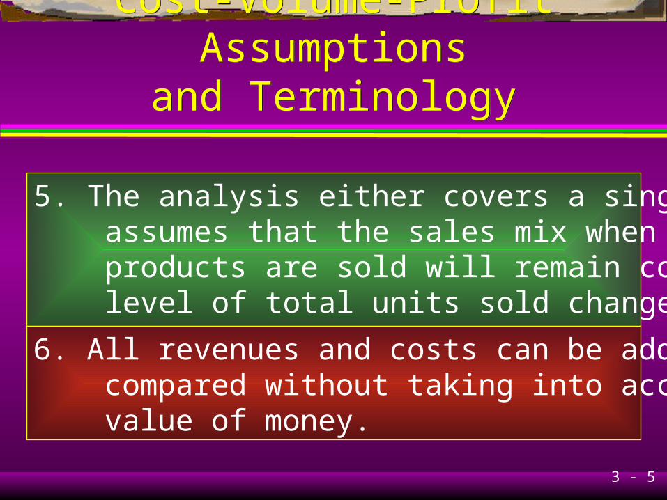
5. The analysis either covers a single product or assumes that the sales mix when multiple products are sold will remain constant as the level of total units sold changes.
6. All revenues and costs can be added and compared without taking into account the time value of money.
3 - 6
Cost-Volume-Profit Assumptionsand Terminology
Cost-Volume-Profit Assumptionsand Terminology
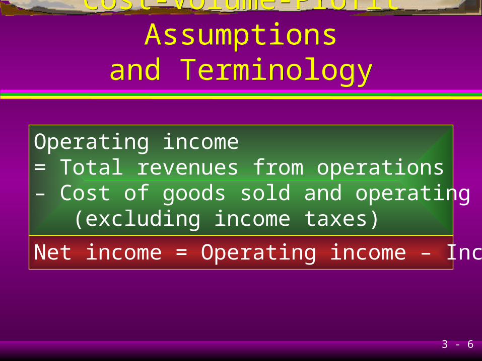
Operating income= Total revenues from operations– Cost of goods sold and operating costs (excluding income taxes)
Net income = Operating income – Income taxes

3 - 7
Learning Objective 2Learning Objective 2
Explain the features
of CVP analysis.
3 - 8
Essentials of Cost-Volume-Profit(CVP) Analysis Example
Essentials of Cost-Volume-Profit(CVP) Analysis Example
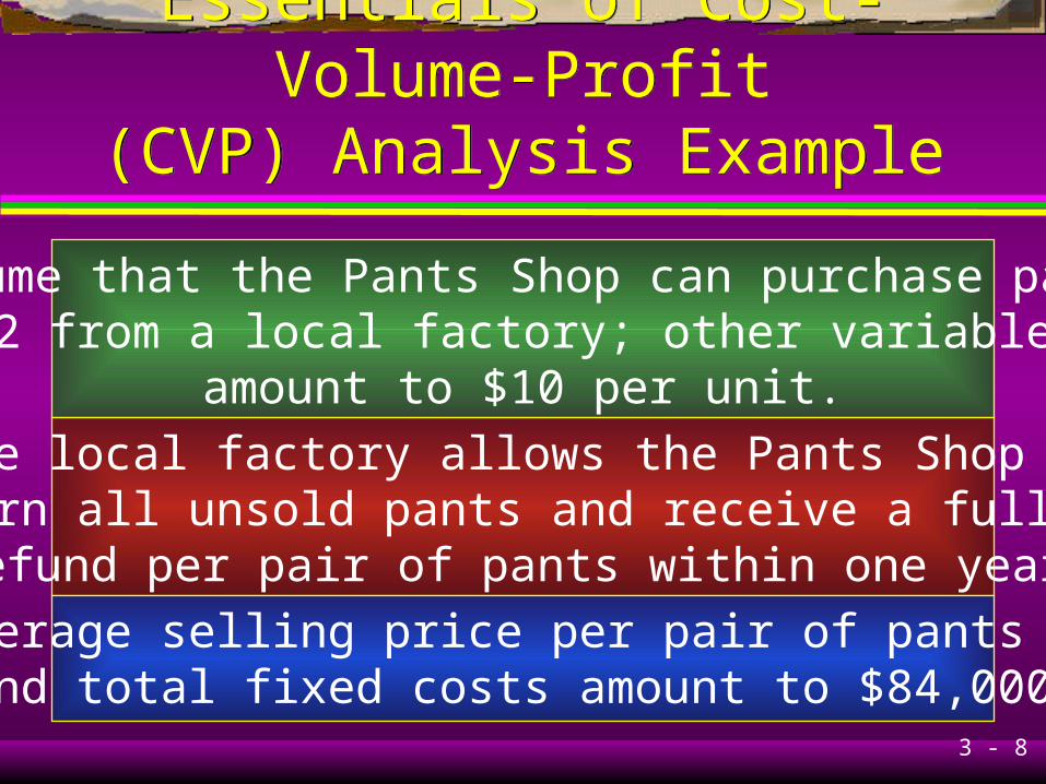
Assume that the Pants Shop can purchase pantsfor $32 from a local factory; other variable costs
amount to $10 per unit.
The local factory allows the Pants Shop toreturn all unsold pants and receive a full $32
refund per pair of pants within one year.
The average selling price per pair of pants is $70and total fixed costs amount to $84,000.
3 - 9
Essentials of Cost-Volume-Profit(CVP) Analysis Example
Essentials of Cost-Volume-Profit(CVP) Analysis Example
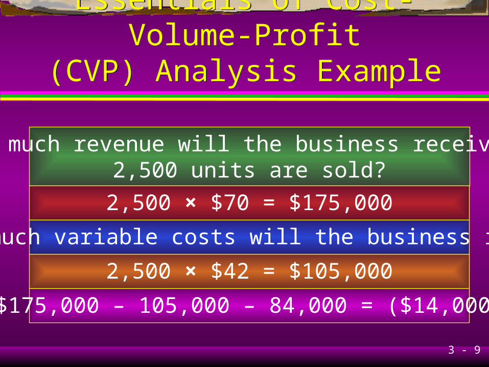
How much revenue will the business receive if2,500 units are sold?
2,500 × $70 = $175,000
How much variable costs will the business incur?
2,500 × $42 = $105,000
$175,000 – 105,000 – 84,000 = ($14,000)
3 - 10
Essentials of Cost-Volume-Profit(CVP) Analysis Example
Essentials of Cost-Volume-Profit(CVP) Analysis Example
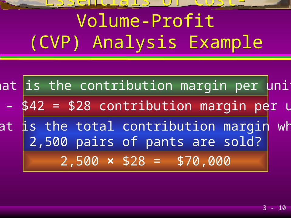
What is the contribution margin per unit?
$70 – $42 = $28 contribution margin per unit
What is the total contribution margin when2,500 pairs of pants are sold?
2,500 × $28 = $70,000
3 - 11
Essentials of Cost-Volume-Profit(CVP) Analysis Example
Essentials of Cost-Volume-Profit(CVP) Analysis Example
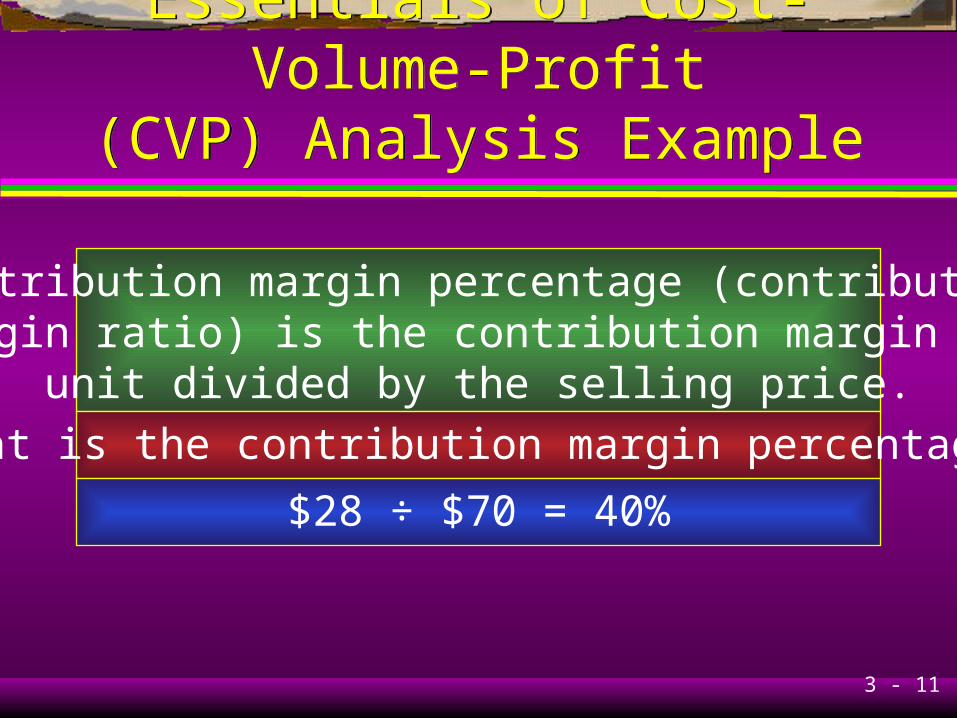
Contribution margin percentage (contributionmargin ratio) is the contribution margin per
unit divided by the selling price.
What is the contribution margin percentage?
$28 ÷ $70 = 40%
3 - 12
Essentials of Cost-Volume-Profit(CVP) Analysis Example
Essentials of Cost-Volume-Profit(CVP) Analysis Example
If the business sells 3,000 pairs of pants,revenues will be $210,000 and contribution
margin would equal 40% × $210,000 = $84,000.
A
FEDERAL RESERVE NOTE
THE UNITED STATES OF AMERICATHE UNITED STATES OF AMERICA
L70744629F
12
1212
12
L70744629F
ONE DOLLARONE DOLLAR
WA SHINGTON, D.C.
TH IS N O TE IS LE GA L TE N DE R
FOR A LL D E B TS , P UB LIC AN D P RIV A TE
S E RIES
19 85
H 293

3 - 13
Learning Objective 3Learning Objective 3
Determine the breakeven point
and output level needed to achieve
a target operating income using
the equation, contribution margin,
and graph methods.
3 - 14
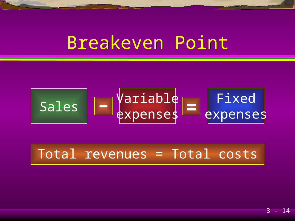
Breakeven PointBreakeven Point
SalesVariableexpenses
Fixedexpenses
– =
Total revenues = Total costs

3 - 15
AbbreviationsAbbreviations
SP = Selling price
VCU = Variable cost per unit
CMU = Contribution margin per unit
CM% = Contribution margin percentage
FC = Fixed costs

3 - 16
AbbreviationsAbbreviations
Q = Quantity of output units sold(and manufactured)
OI = Operating income
TOI = Target operating income
TNI = Target net income
3 - 17
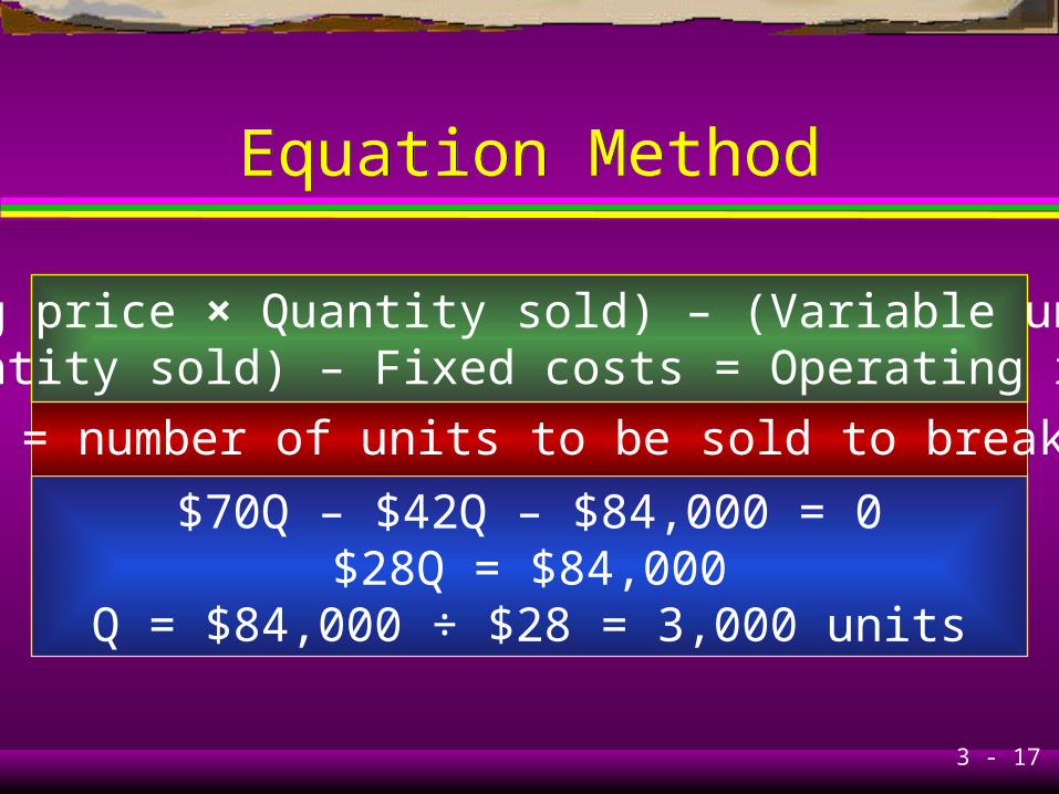
Equation MethodEquation Method
$70Q – $42Q – $84,000 = 0$28Q = $84,000
Q = $84,000 ÷ $28 = 3,000 units
Let Q = number of units to be sold to break even
(Selling price × Quantity sold) – (Variable unit cost× Quantity sold) – Fixed costs = Operating income
3 - 18
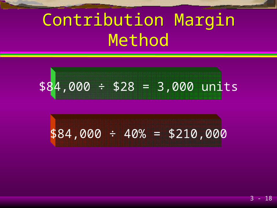
Contribution Margin MethodContribution Margin Method
$84,000 ÷ $28 = 3,000 units
$84,000 ÷ 40% = $210,000

3 - 19
Graph MethodGraph Method
04284
126168210252294336378
0 1000 2000 3000 4000 5000
Units
$(00
0)
Revenue
Total costs
Breakeven
Fixed costs

3 - 20
Target Operating IncomeTarget Operating Income
(Fixed costs + Target operating income)divided either by Contribution margin
percentage or Contribution margin per unit
3 - 21
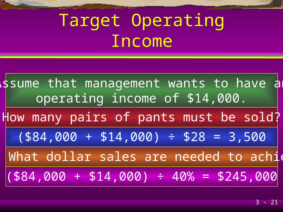
Target Operating IncomeTarget Operating Income
Assume that management wants to have anoperating income of $14,000.
How many pairs of pants must be sold?
($84,000 + $14,000) ÷ $28 = 3,500
What dollar sales are needed to achieve this income?
($84,000 + $14,000) ÷ 40% = $245,000

3 - 22
Learning Objective 4Learning Objective 4
Understand how income
taxes affect CVP analysis.
3 - 23
Target Net Incomeand Income Taxes Example
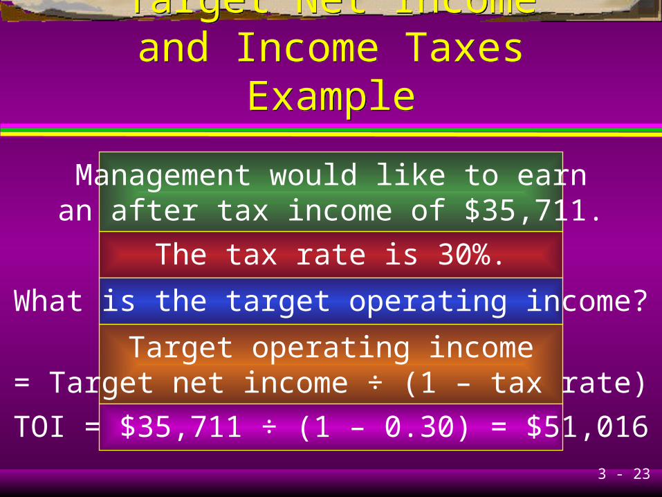
Target Net Incomeand Income Taxes Example
Management would like to earnan after tax income of $35,711.
The tax rate is 30%.
What is the target operating income?
Target operating income= Target net income ÷ (1 – tax rate)
TOI = $35,711 ÷ (1 – 0.30) = $51,016
3 - 24
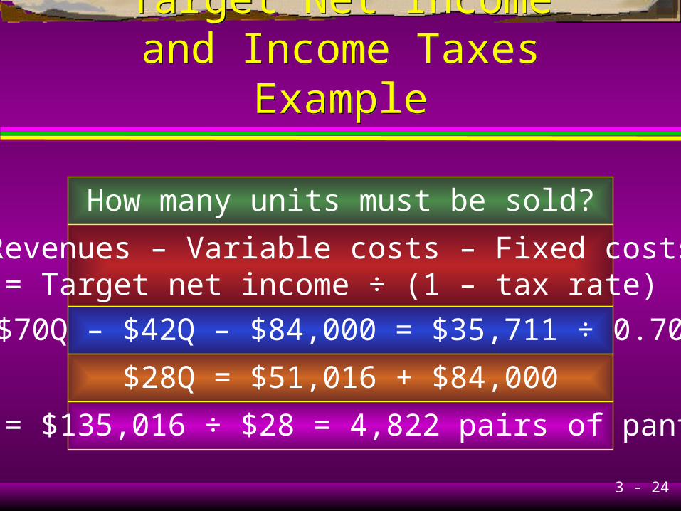
Target Net Incomeand Income Taxes Example
Target Net Incomeand Income Taxes Example
How many units must be sold?
Revenues – Variable costs – Fixed costs= Target net income ÷ (1 – tax rate)
$70Q – $42Q – $84,000 = $35,711 ÷ 0.70
$28Q = $51,016 + $84,000
Q = $135,016 ÷ $28 = 4,822 pairs of pants
3 - 25
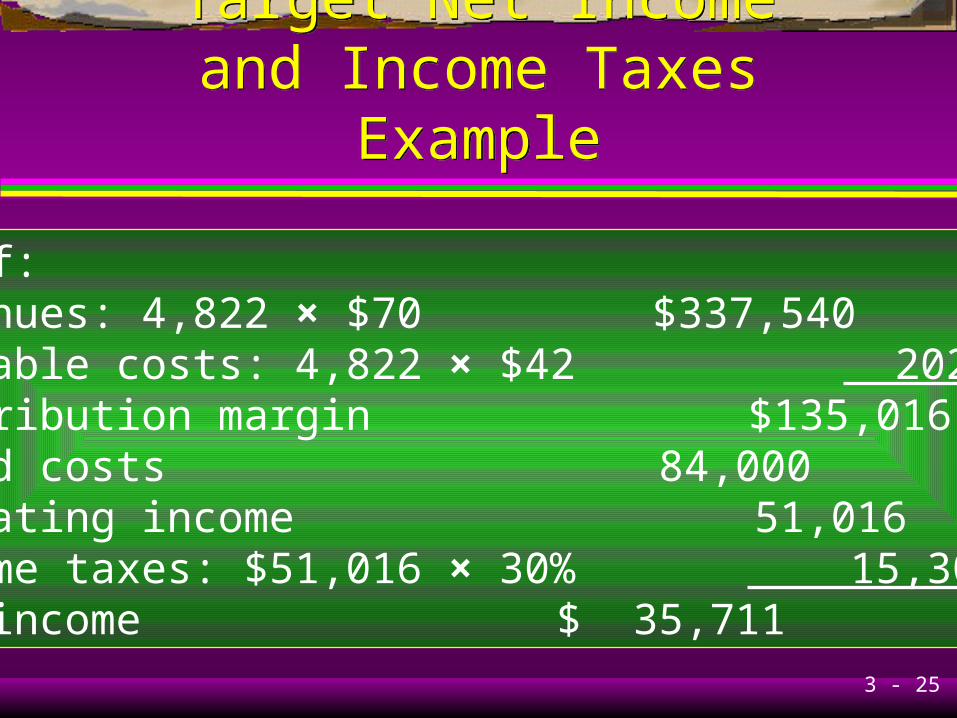
Target Net Incomeand Income Taxes Example
Target Net Incomeand Income Taxes Example
Proof:Revenues: 4,822 × $70 $337,540Variable costs: 4,822 × $42 202,524Contribution margin $135,016Fixed costs 84,000Operating income 51,016Income taxes: $51,016 × 30% 15,305Net income $ 35,711
3 - 26
Learning Objective 5Learning Objective 5
Explain CVP analysis
in decision making and
how sensitivity analysis helps
managers cope with uncertainty.

3 - 27
Using CVP Analysis ExampleUsing CVP Analysis Example
Suppose the management anticipatesselling 3,200 pairs of pants.
Management is considering an advertisingcampaign that would cost $10,000.
It is anticipated that the advertising willincrease sales to 4,000 units.
Should the business advertise?

3 - 28
Using CVP Analysis ExampleUsing CVP Analysis Example
3,200 pairs of pants sold with no advertising:
Contribution margin $89,600Fixed costs 84,000Operating income $ 5,600
4,000 pairs of pants sold with advertising:
Contribution margin $112,000Fixed costs 94,000Operating income $ 18,000

3 - 29
Using CVP Analysis ExampleUsing CVP Analysis Example
Instead of advertising, management isconsidering reducing the selling price
to $61 per pair of pants.
It is anticipated that this will increasesales to 4,500 units.
Should management decrease the sellingprice per pair of pants to $61?

3 - 30
Using CVP Analysis ExampleUsing CVP Analysis Example
3,200 pairs of pants sold with no changein the selling price:
Operating income = $5,600
4,500 pairs of pants sold at a reduced selling price:
Contribution margin: (4,500 × $19) $85,500Fixed costs 84,000Operating income $ 1,500

3 - 31
Sensitivity Analysis andUncertainty Example
Sensitivity Analysis andUncertainty Example
Assume that the Pants Shop can sell4,000 pairs of pants.
Fixed costs are $84,000.
Contribution margin ratio is 40%.
At the present time the business cannothandle more than 3,500 pairs of pants.
3 - 32
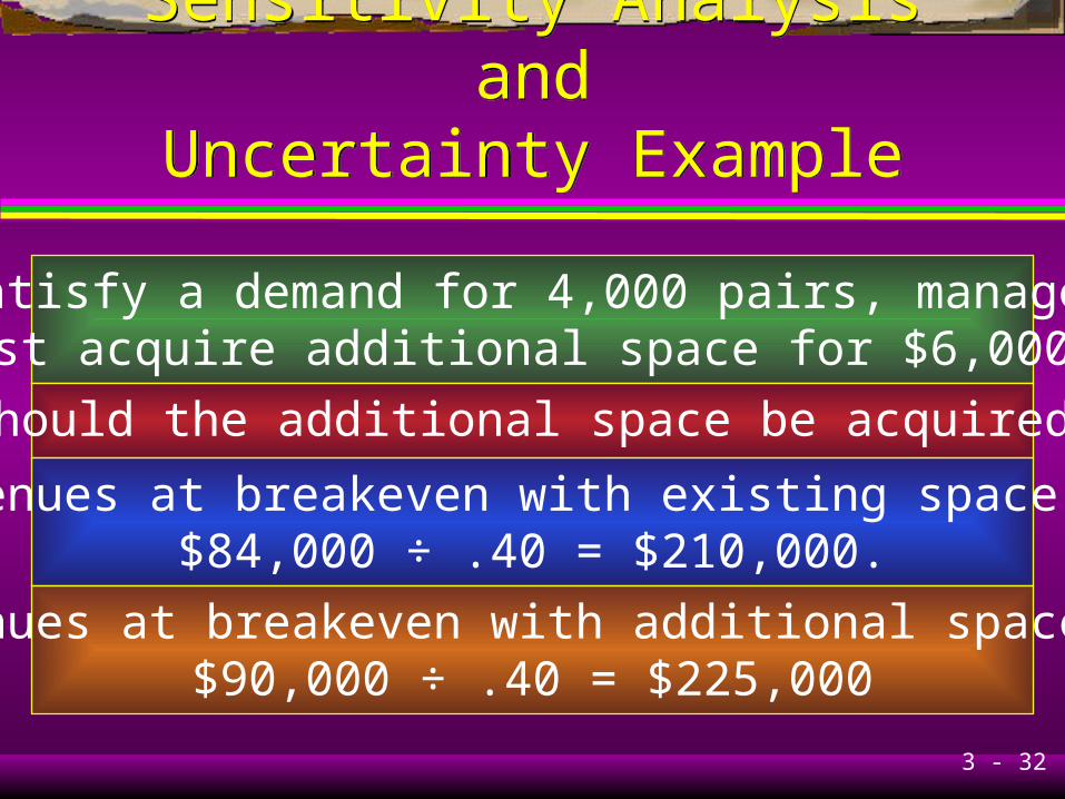
Sensitivity Analysis andUncertainty Example
Sensitivity Analysis andUncertainty Example
To satisfy a demand for 4,000 pairs, managementmust acquire additional space for $6,000.
Should the additional space be acquired?
Revenues at breakeven with existing space are$84,000 ÷ .40 = $210,000.
Revenues at breakeven with additional space are$90,000 ÷ .40 = $225,000

3 - 33
Sensitivity Analysis andUncertainty Example
Sensitivity Analysis andUncertainty Example
Operating income at $245,000 revenues withexisting space = ($245,000 × .40)
– $84,000 = $14,000.
(3,500 pairs of pants × $28) – $84,000 = $14,000
3 - 34
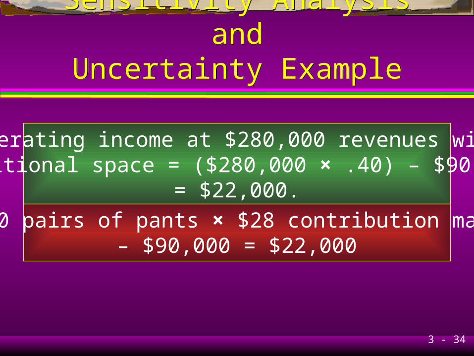
Sensitivity Analysis andUncertainty Example
Sensitivity Analysis andUncertainty Example
Operating income at $280,000 revenues withadditional space = ($280,000 × .40) – $90,000
= $22,000.
(4,000 pairs of pants × $28 contribution margin)– $90,000 = $22,000

3 - 35
Learning Objective 6Learning Objective 6
Use CVP analysis to plan
fixed and variable costs.
3 - 36
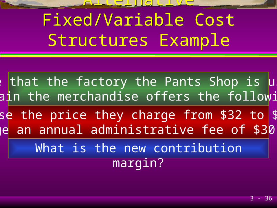
Alternative Fixed/Variable CostStructures Example
Alternative Fixed/Variable CostStructures Example
What is the new contribution margin?
Decrease the price they charge from $32 to $25 andcharge an annual administrative fee of $30,000.
Suppose that the factory the Pants Shop is using toobtain the merchandise offers the following:

3 - 37
Alternative Fixed/Variable Cost Structures Example
Alternative Fixed/Variable Cost Structures Example
$70 – ($25 + $10) = $35
Contribution margin increases from $28 to $35.
What is the contribution margin percentage?
$35 ÷ $70 = 50%
What are the new fixed costs?
$84,000 + $30,000 = $114,000

3 - 38
Alternative Fixed/Variable Cost Structures Example
Alternative Fixed/Variable Cost Structures Example
Management questions what sales volumewould yield an identical operating income
regardless of the arrangement.
28x – 84,000 = 35x – 114,000
114,000 – 84,000 = 35x – 28x
7x = 30,000
x = 4,286 pairs of pants

3 - 39
Alternative Fixed/Variable Cost Structures Example
Alternative Fixed/Variable Cost Structures Example
Cost with existing arrangement= Cost with new arrangement
.60x + 84,000 = .50x + 114,000
.10x = $30,000 x = $300,000
($300,000 × .40) – $ 84,000 = $36,000
($300,000 × .50) – $114,000 = $36,000
3 - 40
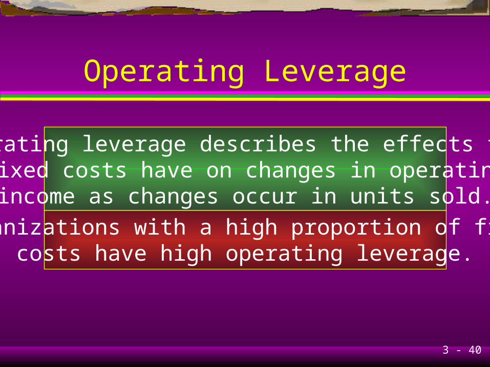
Operating LeverageOperating Leverage
Operating leverage describes the effects thatfixed costs have on changes in operatingincome as changes occur in units sold.
Organizations with a high proportion of fixedcosts have high operating leverage.
3 - 41
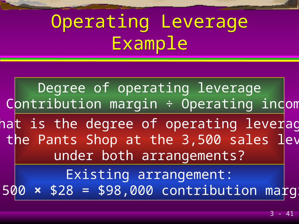
Operating Leverage ExampleOperating Leverage Example
Degree of operating leverage= Contribution margin ÷ Operating income
What is the degree of operating leverageof the Pants Shop at the 3,500 sales level
under both arrangements?
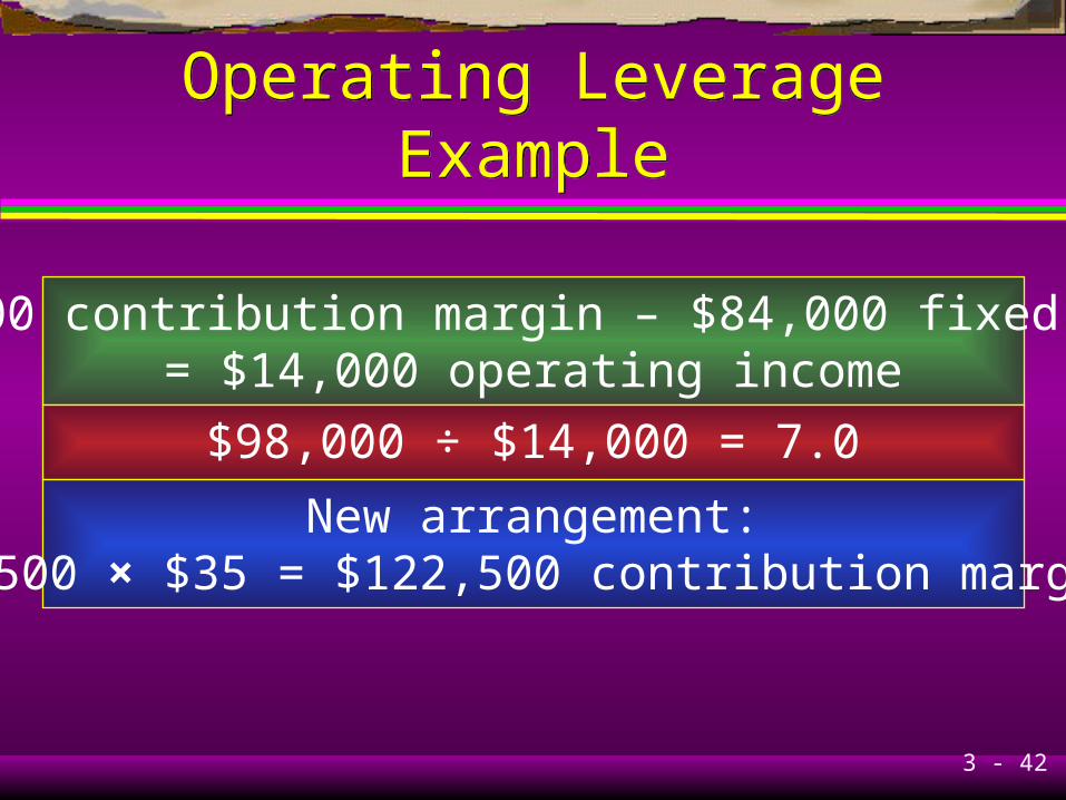
Existing arrangement:3,500 × $28 = $98,000 contribution margin
3 - 42
Operating Leverage ExampleOperating Leverage Example
$98,000 contribution margin – $84,000 fixed costs= $14,000 operating income
$98,000 ÷ $14,000 = 7.0
New arrangement:3,500 × $35 = $122,500 contribution margin
3 - 43
Operating Leverage ExampleOperating Leverage Example
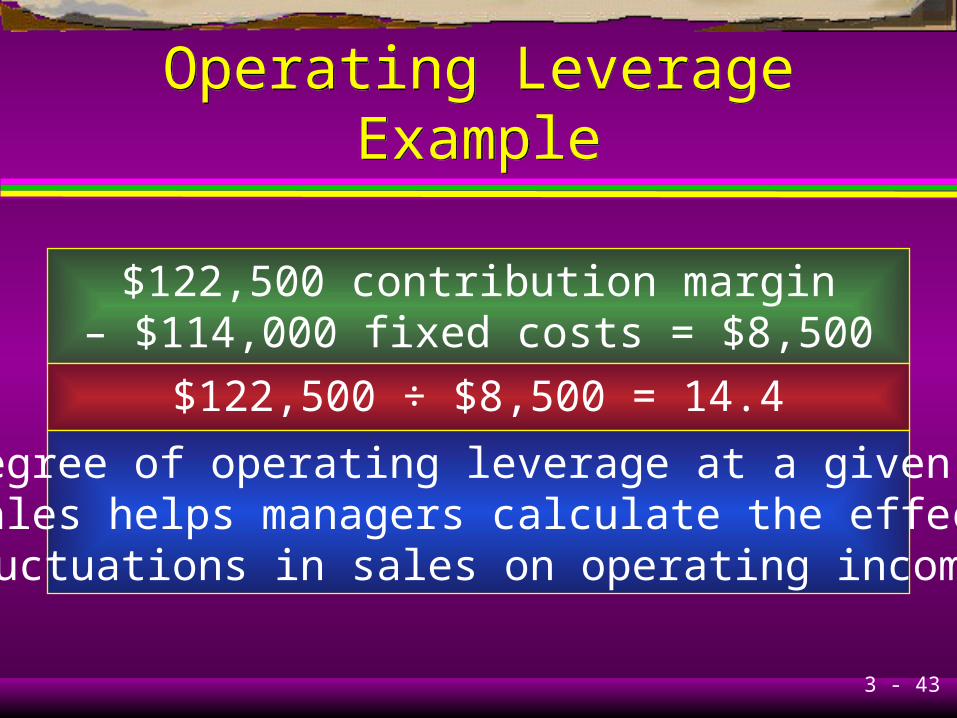
$122,500 contribution margin– $114,000 fixed costs = $8,500
$122,500 ÷ $8,500 = 14.4
The degree of operating leverage at a given levelof sales helps managers calculate the effect of
fluctuations in sales on operating income.
3 - 44
Learning Objective 7Learning Objective 7
Apply CVP analysis to a company
producing different products.
3 - 45
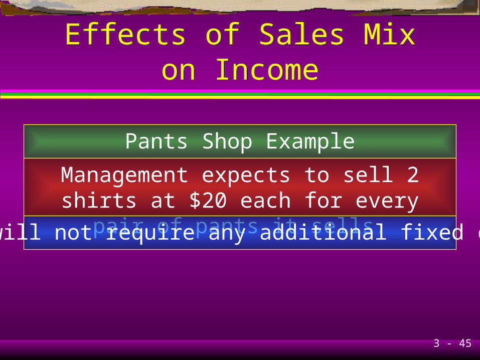
Effects of Sales Mix on IncomeEffects of Sales Mix on Income
Pants Shop Example
Management expects to sell 2 shirts at $20 each for every pair of pants it sells.
This will not require any additional fixed costs.

3 - 46
Effects of Sales Mix on IncomeEffects of Sales Mix on Income
What is the contribution margin of the mix?
Contribution margin per shirt: $20 – $9 = $11
$28 + (2 × $11) = $28 + $22 = $50
3 - 47
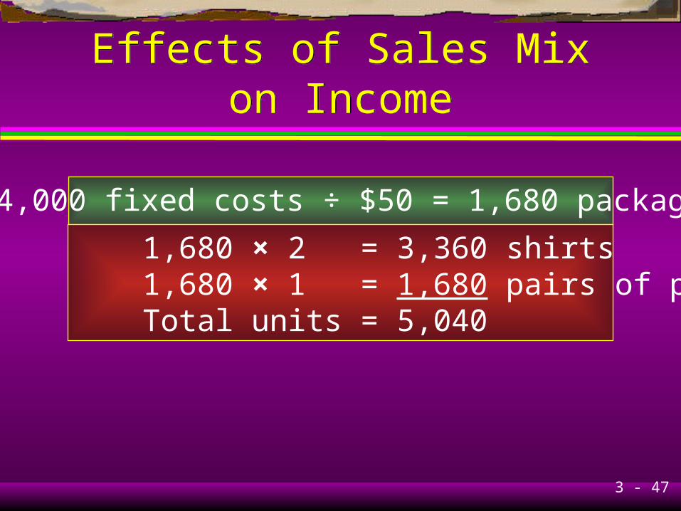
Effects of Sales Mix on IncomeEffects of Sales Mix on Income
$84,000 fixed costs ÷ $50 = 1,680 packages
1,680 × 2 = 3,360 shirts1,680 × 1 = 1,680 pairs of pantsTotal units = 5,040
3 - 48
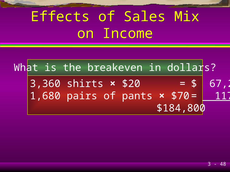
Effects of Sales Mix on IncomeEffects of Sales Mix on Income
What is the breakeven in dollars?
3,360 shirts × $20 = $ 67,2001,680 pairs of pants × $70 = 117,600
$184,800

3 - 49
Effects of Sales Mix on IncomeEffects of Sales Mix on Income
What is the weighted-average budgeted contribution margin?
Pants: 1 × $28 + Shirts: 2 × $11
= $50 ÷ 3 = $16.667
3 - 50
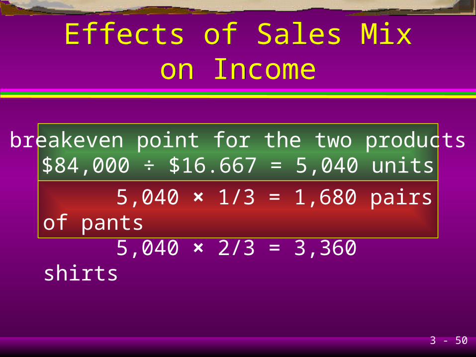
Effects of Sales Mix on IncomeEffects of Sales Mix on Income
The breakeven point for the two products is:$84,000 ÷ $16.667 = 5,040 units
5,040 × 1/3 = 1,680 pairs of pants 5,040 × 2/3 = 3,360 shirts
3 - 51
Effects of Sales Mix on IncomeEffects of Sales Mix on Income
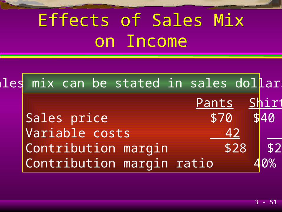
Sales mix can be stated in sales dollars:
Pants ShirtsSales price $70 $40Variable costs 42 18Contribution margin $28 $22Contribution margin ratio 40% 55%

3 - 52
Effects of Sales Mix on IncomeEffects of Sales Mix on Income
Assume the sales mix in dollarsis 63.6% pants and 36.4% shirts.
Weighted contribution would be:40% × 63.6% = 25.44% pants55% × 36.4% = 20.02% shirts
45.46%
3 - 53
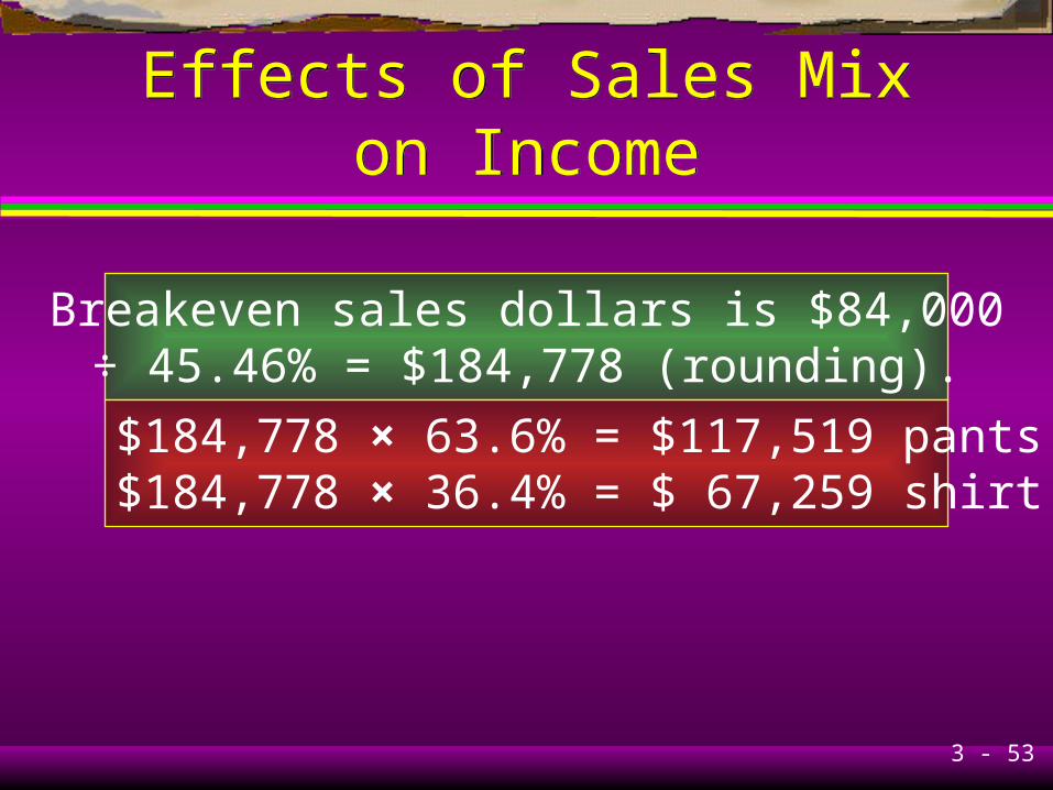
Effects of Sales Mix on IncomeEffects of Sales Mix on Income
Breakeven sales dollars is $84,000÷ 45.46% = $184,778 (rounding).
$184,778 × 63.6% = $117,519 pants sales$184,778 × 36.4% = $ 67,259 shirt sales
3 - 54
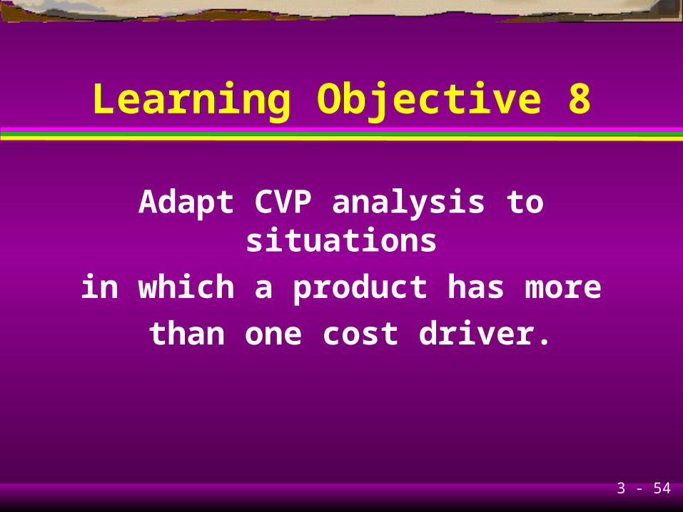
Learning Objective 8Learning Objective 8
Adapt CVP analysis to situations
in which a product has more
than one cost driver.

3 - 55
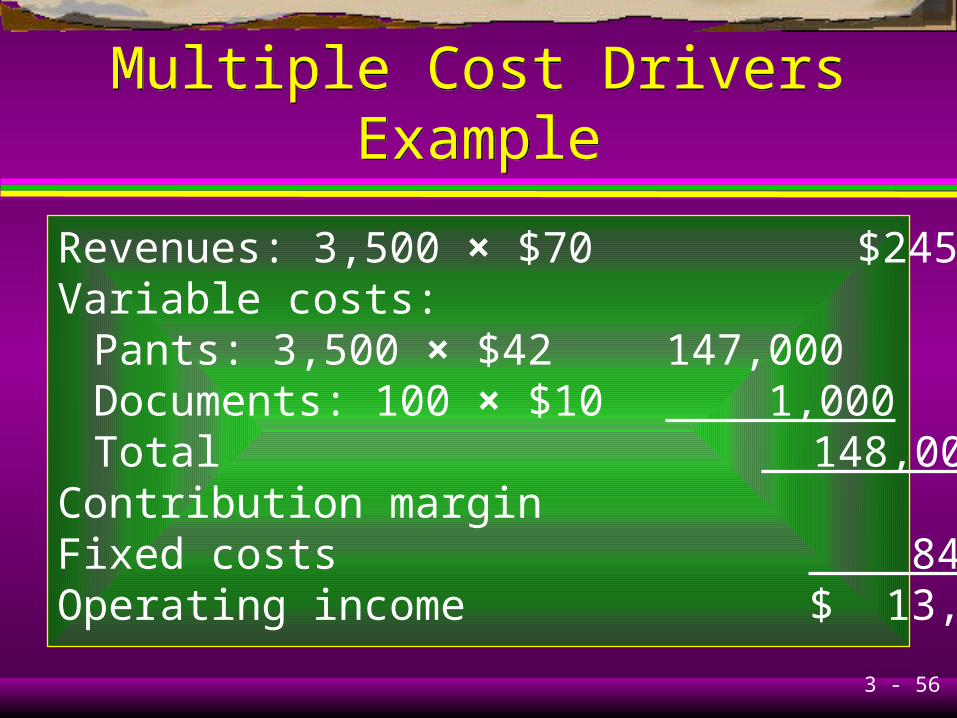
Multiple Cost Drivers ExampleMultiple Cost Drivers Example
Suppose that the business will incur an additionalcost of $10 for preparing documents associated
with the sale of pants to various customers.
Assume that the business sells 3,500pants to 100 different customers.
What is the operating income from this sale?
3 - 56
Multiple Cost Drivers ExampleMultiple Cost Drivers Example
Revenues: 3,500 × $70 $245,000Variable costs:
Pants: 3,500 × $42 147,000Documents: 100 × $10 1,000Total 148,000
Contribution margin 97,000Fixed costs 84,000Operating income $ 13,000
3 - 57
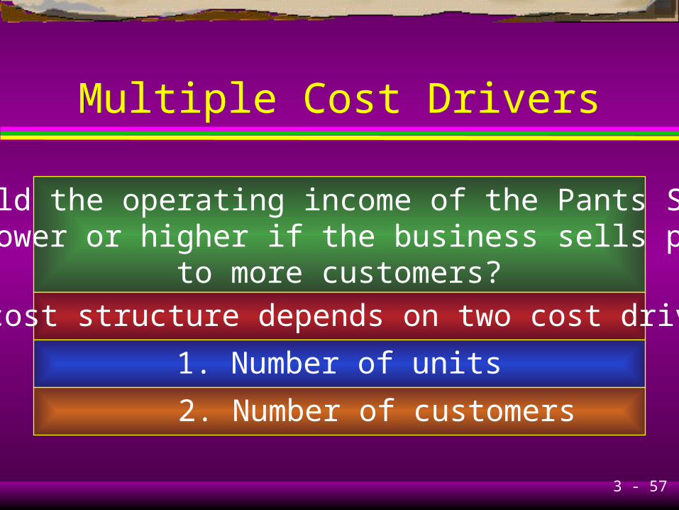
Multiple Cost DriversMultiple Cost Drivers
Would the operating income of the Pants Shopbe lower or higher if the business sells pants
to more customers?
The cost structure depends on two cost drivers:
1. Number of units
2. Number of customers

3 - 58
Learning Objective 9Learning Objective 9
Distinguish between
contribution margin
and gross margin.
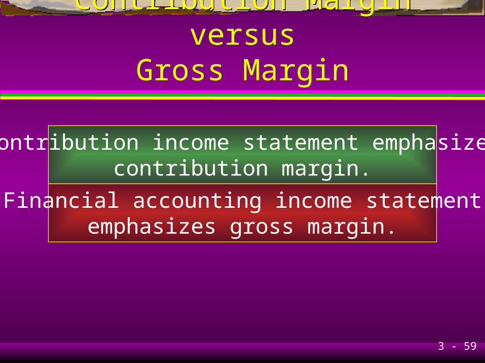
3 - 59
Contribution Margin versusGross Margin
Contribution Margin versusGross Margin
Contribution income statement emphasizescontribution margin.
Financial accounting income statementemphasizes gross margin.

3 - 60
End of Chapter 3End of Chapter 3


