2QRWNCVKQP CPF 'EQPQOKE 2TQLGEVKQPU HQT VJG 5VCVG … · l 7deoh ri &rqwhqwv /lvw ri 7deohv ll

Population and Economic Projections for the State of Hawaii to 2045

June 2018

Research and Economic Analysis Division Department of Business, Economic Development

and Tourism STATE of HAWAII

This report was prepared by Dr. Yang-Seon Kim, Research and Statistics Officer, and Dr. Jie Bai, Economist, under the direction of Dr. Eugene Tian, Division Administrator. DBEDT would like to thank many agencies and individuals who provided comments and suggestions on the projections.

i

Table of Contents

List of Tables.................................................................................................................. ii

List of Figures ................................................................................................................ ii

I. Summary of Projections ............................................................................................... 1

1. Population .................................................................................................................. 1

2. Gross Domestic Product and Personal Income .......................................................... 7

3. Jobs and Employment ................................................................................................ 9

4. Tourism .................................................................................................................... 11

II. Hawaii Population and Economic Projection Methodology .................................. 13

1. The Demographic Module ...................................................................................... 14

Fertility Rates .......................................................................................................... 14 Life Tables and Survival Rates ............................................................................... 17 Net Migration .......................................................................................................... 20

2. The Economic Module ............................................................................................ 22

Projection of GDP and Final Demand ..................................................................... 22 Personal Consumption Expenditures ............................................................... 22 Private Investment ............................................................................................ 23 Government Spending ...................................................................................... 23 Exports ............................................................................................................. 24 Imports ............................................................................................................. 24

Projections of Output .............................................................................................. 24 Projections of Jobs .................................................................................................. 25 Projections of Employment ..................................................................................... 26 Projections of Income .............................................................................................. 26

Labor Income ................................................................................................... 26 Transfer Payments ............................................................................................ 27 Property Income ............................................................................................... 27 Contributions for Government Social Insurance ............................................. 27 Disposable Income ........................................................................................... 27

Tourism Projections ................................................................................................ 27 Visitor Arrival Projections ............................................................................... 28 Visitor Days and Daily Visitor Census ............................................................ 29 Visitor Expenditures......................................................................................... 30

ii

List of Tables

Table 1- 1. Resident Population by County: 1980-2045..................................................... 2

Table 1- 2. De Facto Population by County: 1980-2045 .................................................... 3

Table 1- 3. Projections of Real GDP .................................................................................. 7

Table 1- 4. Actual and Projected Personal Income (in millions of 2012 dollars) ............... 8

Table 1- 5. Actual and Projected Civilian Jobs................................................................. 10

Table 1- 6. Actual and Projected Civilian Employed ....................................................... 11

Table 2- 1. Total Fertility Rate: History and Projection ................................................... 17

Table 2- 2. Life Expectancy at Birth for the U.S. and Hawaii: 1980-2014 (Total Residents) .................................................................................................................. 18

Table 2- 3. Projected Life Expectancy at Birth for Hawaii: 2014 and 2045 (Other Civilian) .................................................................................................................... 19

Table 2- 4. Estimation and Projection of Net-Migration .................................................. 21

Table 2- 5. Future Growth of Visitor Arrivals: 2017-2045 .............................................. 28

Table 2- 6. Assumptions Employed for the Projections of Visitor Arrivals1 ................... 29

Table 2- 7. Assumptions Employed for the Projections of Visitor Days1 ........................ 29

Table 2- 8. Assumptions Employed for the Projections of Visitor Expenditures1 ........... 30

List of Figures

Figure 1- 1. Resident Population by Major Age Group: 1980 to 2045............................... 4

Figure 1- 2. Dependency Ratios: Historical Trend and Projection ..................................... 5

Figure 1- 3. Projected Age Composition of Elderly Population in Hawaii: 2010-2045 ..... 5

Figure 1- 4. Age Distribution of Resident Population in Hawaii: 1980 to 2045 ................ 6

Figure 1- 5. Average Annual Growth of Real Personal Income for the State .................... 8

Figure 1- 6. Average Annual Growth of Total Civilian Jobs for the State ......................... 9

Figure 1- 7. Visitor Arrivals by Air, History and Projection ............................................ 12

Figure 2- 1. Trend of Fertility Rates in Hawaii and the U.S. ............................................ 16

Figure 2- 2. Fertility Rates in Hawaii by the Age of Mother, 2008 vs. 2016 ................... 16

Figure 2- 3. Survival Rates in Hawaii; 1990 vs. 2014 ...................................................... 18

Figure 2- 4. Age Distribution of Migrants ........................................................................ 20

1

This report presents the results and methodology of the 2045 Series of the DBEDT Population and Economic Projections for the State of Hawaii and its four counties. This is the ninth in a series of long-range projections dating back to the first report published in 1978. The 2045 Series uses the detailed population characteristics from the 2010 Decennial Census, 2016 vintage intercensal population estimates by the U.S. Census Bureau, 2016 estimates of economic variables, and input-output (I-O) tables based on the 2012 Economic Census as baseline data for the projection.

It should be noted that these projections are neither targets nor goals. They are DBEDT’s best estimates of likely trends in important population and economic variables based on currently available information. The accuracy of these projections depends on the degree to which historical trends provide guides to the future, changing external conditions, infrastructure capacity, and other supply constraints which have not been incorporated into the model.

Section 1 of this report summarizes the population and economic projections for the state and counties. Section 2 describes the methodology and assumptions that were used to produce the projections. The appendix tables contain detailed projections.

I. Summary of Projections

1. Population

The resident population of Hawaii, which includes active-duty military personnel and their dependents as well as other civilian population, is projected to increase from 1.43 million in 2016 to 1.65 million in 2045, an average growth rate of 0.5 percent per year over the projection period.

The size of military population in Hawaii has been determined mostly as the result of national defense consideration. Without a clear known direction of the future level of military personnel in Hawaii this projection was produced based on the assumption that the size of military population in Hawaii will stay at its past five-year average as it has been at a stable level in the past five years.

The size and composition of other civilian population were determined by three components: births, deaths, and net migration. Net-migration to other civilian population was assumed to remain at 4,800 per year during the projection period, which was the average size of net-migration added to other civilian population annually during the 1980-2016 period. Natural population increase (i.e., total births minus total deaths) has been decreasing due to population aging. This trend is expected to continue in the future resulting in population growing at a moderate and diminishing rate over the projection period. The methodology and detailed

2

discussion on the assumptions made on fertility, mortality, and migration are included in the methodology section.

Table 1- 1 presents the projection of total resident population by county. As has been the case in the previous DBEDT long-range projections, the Neighbor Island counties are projected to have higher population growth than Honolulu County during the projection period. The resident population of Honolulu County is projected to grow at an annual rate of 0.3 percent during the 2016 to 2045 period, while Hawaii County is projected to grow at 1.1 percent, Maui County at 0.9 percent, and Kauai County at 0.8 percent annually respectively.

The combined share of three neighbor islands in total Hawaii population has increased from 21.1 percent in 1980 to 30.5 percent in 2016. It was the result of faster population growths observed in the neighbor islands in the past decades. The population share of the neighbor islands are projected to further increase to 34.9 percent by 2045 as the faster population growths in the neighbor islands are projected to continue during the projection period.

Table 1- 1. Resident Population by County: 1980-2045

Year State Total

Hawaii County

Honolulu County

Kauai County

Maui County

19801 968,500 92,900 764,600 39,400 71,600

19901 1,113,491 121,572 838,534 51,676 101,709

20001 1,213,519 149,244 876,629 58,568 129,078

20101 1,363,621 185,406 955,775 67,226 155,214

20161 1,428,557 198,449 992,605 72,029 165,474

20252 1,514,700 222,400 1,032,700 78,000 181,600

20352 1,592,700 248,500 1,062,100 84,300 197,800

20452 1,648,600 273,200 1,073,800 90,000 211,500

Average annual growth rate (%)

1980-1990 1.4 2.7 0.9 2.7 3.6 1990-2000 0.9 2.1 0.4 1.3 2.4 2000-2010 1.2 2.2 0.9 1.4 1.9 2010-2016 0.8 1.1 0.6 1.2 1.1

2016-2025 0.7 1.3 0.4 0.9 1.0 2025-2035 0.5 1.1 0.3 0.8 0.9 2035-2045 0.3 1.0 0.1 0.7 0.7

1 July estimates by the U.S. Census Bureau 2 DBEDT projections, figures presented here can be different from those in the appendix tables because of rounding.

Due to the important role of tourism in the state of Hawaii De Facto population, which counts those who physically present in a given area at a given time, is often served as a more useful

3

measure for planning purpose. De Facto population can be calculated from resident population by adding visitors who stayed in the area and subtracting residents who were temporarily away from home in a typical day of the year. In 2016, De Facto population was estimated 11 percent higher than resident population statewide. However, the difference varied significantly by county. De Facto population was more than 30 percent higher than resident population in Maui and Kauai County while it was 5.7 percent and 12.1 percent higher in Honolulu and Hawaii County respectively. For the future years, De Facto population is projected to grow slightly faster than resident population in all counties mainly due to tourism projected to grow faster than population growth over the projection period.

Table 1- 2. De Facto Population by County: 1980-2045

Year State Total

Hawaii County

Honolulu County

Kauai County

Maui County

1980 1,054,218 99,181 822,408 46,341 86,288

1990 1,257,319 137,103 913,268 68,558 138,390

2000 1,336,005 166,429 926,192 74,734 168,650

2010 1,468,677 202,682 988,095 83,516 194,384

2016 1,583,139 222,485 1,048,965 93,630 218,059

20251 1,695,200 252,100 1,094,000 103,800 245,300

20351 1,792,100 282,600 1,125,900 113,100 270,500

20451 1,866,500 311,900 1,139,400 121,800 293,300

Average annual growth rate (%)

1980-1990 1.8 3.3 1.1 4.0 4.8 1990-2000 0.6 2.0 0.1 0.9 2.0 2000-2010 1.0 2.0 0.6 1.1 1.4 2010-2016 1.3 1.6 1.0 1.9 1.9 2016-2025 0.8 1.4 0.5 1.1 1.3 2025-2035 0.6 1.1 0.3 0.9 1.0 2035-2045 0.4 1.0 0.1 0.7 0.8

1 DBEDT projections, figures presented here can be different from those in the appendix tables because of rounding.

Population aging is one of the most prominent features of Hawaii’s population trend. Increasing its size by 3.3 percent annually on average, the share of elderly population, aged 65 years and over, of Hawaii total population increased from 7.9 percent in 1980 to 17.1 percent in 2016. The fast growth in the elderly population is expected to continue until around 2030 when the age group will start to slow down its growth. By 2045, the share of elderly population is projected to increase to 23.8 percent. All other age groups will also grow over the projection period, but their shares of total population will diminish over time.

4

Figure 1- 1. Resident Population by Major Age Group: 1980 to 2045

Dependency ratio can be calculated to measure the burden on productive population in an economy. By comparing the size of dependent population (children aged between 0 and 17 and elderly population aged 65 and over) to the size of active working-age population (people aged 18-64), total dependency ratio provides a rough indicator of the burden on the working population in the economy. Another useful measure of dependency is old age dependency ratio, which is calculated by dividing the elderly population (65 and over) by the working age population (aged 18-64). Figure 1- 2 presents these two most widely used dependency ratios. Compared to the U.S. average, in 2016, total dependency ratio of Hawaii was 1.6 percentage point higher while old-age dependency ratio was 3.2 percentage point higher. As presented in Figure 1- 2, both dependency ratios in Hawaii are projected to increase until around 2035 before they level off.

28.6%25.4%24.4%

21.6%21.3%

20.3%

0%

10%

20%

30%

40%

50%

-

100,000

200,000

300,000

400,000

500,000

600,000

1980 1990 2000 2016 2030 2045

Age 0-17

Number of Residents share of total

44.9% 45.2%

39.4%36.0%

34.1% 32.7%

0%

10%

20%

30%

40%

50%

-

100,000

200,000

300,000

400,000

500,000

600,000

1980 1990 2000 2016 2030 2045

Age 18-44


18.6%18.2%22.9%

25.4%22.0% 23.2%

0%

10%

20%

30%

40%

50%

-

100,000

200,000

300,000

400,000

500,000

600,000

1980 1990 2000 2016 2030 2045

Age 45-64


7.9%11.2%13.3%

17.1%22.6%

23.8%

0%

10%

20%

30%

40%

50%

-

100,000

200,000

300,000

400,000

500,000

600,000

1980 1990 2000 2016 2030 2045

Age 65 and over


5

Figure 1- 2. Dependency Ratios: Historical Trend and Projection

Figure 1- 4 in the next page compares age structure of the population in Hawaii from 1980 to 2045 by 5 age group and by gender. Rapid growth is expected especially in the population group aged 75 years and over, and the aging of population will be more evident in female population. Aging within the elderly population is another phenomenon that will be clearly observed in the future years. In 2016, more than a half of the elderly population (aged 65 years and over) was in the 65-74 age range while 15.6 percent was in “85 and over”. By 2045, the share of the population aged 65-74 is projected to decrease to 38.4 percent of total elderly population while the population aged 85 years and over is projected to increase its share to 27.4 percent.

Projections of population for the state of Hawaii and its four counties are presented by selected characteristics and by five-year age groups in Appendix Tables A-2 through A-21.

Figure 1- 3. Projected Age Composition of Elderly Population in Hawaii: 2010-2045

24.6%

61.4%

27.8%

63.0%

Old agedependency

ratio

Totaldependency

ratio

US Hawaii

0%

20%

40%

60%

80%

100%

1980 1990 2000 2010 2016 2020 2025 2030 2035 2040 2045

Old age dependency ratio, HawaiiTotal dependency ratio, Hawaii

65-74

75-84

85 and over

0%

10%

20%

30%

40%

50%

60%

70%

80%

90%

100%

2010 2015 2020 2025 2030 2035 2040 2045

6

Figure 1- 4. Age Distribution of Resident Population in Hawaii: 1980 to 2045

1 Source: 1980, 2000 Decennial Census, U.S. Census Bureau 2 Source: Estimates by U.S. Census Bureau 3 DBEDT projections

70,000 35,000 0 35,000 70,000

0-45-9

10-1415-1920-2425-2930-3435-3940-4445-4950-5455-5960-6465-6970-7475-7980-84

85plus

19801

Female

persons

70,000 35,000 0 35,000 70,000

0-45-9

10-1415-1920-2425-2930-3435-3940-4445-4950-5455-5960-6465-6970-7475-7980-84

85plus

20001

Male Female

persons

70,000 35,000 0 35,000 70,000

0-4 5-9

10-14 15-19 20-24 25-29 30-34 35-39 40-44 45-49 50-54 55-59 60-64 65-69 70-74 75-79 80-84

85plus

20162

persons

Male Female

70,000 35,000 0 35,000 70,000

0-4 5-9

10-14 15-19 20-24 25-29 30-34 35-39 40-44 45-49 50-54 55-59 60-64 65-69 70-74 75-79 80-84

85plus

persons

20453

Male Female

Male

7

2. Gross Domestic Product and Personal Income

The Hawaii economy growth is expected to be gradual over the coming decades. The prospects for more rapid growth is limited by the structural factor of an aging population. Projections of gross domestic product (GDP) and personal income are summarized in Table 1- 3 and Table 1- 4.

The real gross domestic product of Hawaii is forecast to grow at 1.7 percent per year over the projection period. The growth of GDP depends on demand from outside the region as well as local consumption and investment. Demand from outside the region is assumed exogenously as it is determined by factors that are difficult to incorporate in the model.

Table 1- 3. Projections of Real GDP

Real GDP (State total, in millions of 2012 dollars)

2016 2020 2025 2030 2035 2040 2045

80,300 86,500 94,700 103,600 112,500 121,700 131,500

Average Annual Growth Rate

2016-2020 2020-2025 2025-2030 2030-2035 2035-2040 2040-2045

1.9% 1.8% 1.8% 1.7% 1.6% 1.6%

This projection takes into accounts the slowdown in construction activities. After a few years’ expansion, both the private building authorization and government contracts awarded have recently been decreasing. The projection also anticipates an overall reduction in the long-term growth of investment, leading to a forecast of a moderate GDP growth.

Another factor that contributes to the moderate level of GDP growth is an anticipation of slow tourism growth. As presented in the tourism section and Table A-60 in the Appendix, tourism expenditures are projected to grow at lower than one percent annually in real terms on average for the period of 2016-2045.

Hawaii’s total personal income is forecast to grow at an annual rate of 1.96 percent in real terms over the projection period. With a growing population, per capita personal income will grow at a lower rate than that of total personal income. In particular, the Neighbor Islands are expected to experience relatively low growth of per capita personal income as a result of higher rates of population growth.

Among the components of personal income, transfer payments are expected to grow at a faster rate than other components because of increased retirement incomes of the aging population. As a result, the share of transfer payments to total personal income is projected to increase from 15.7 percent in 2016 to 20.5 percent in 2045, while the share of labor income, the largest component of personal income, is projected to decrease from 71.2 percent in 2016 to 65.9 percent in 2045.

8

Detailed historical series and projections of personal income are reported in Appendix Tables A-49 through A-54.

Figure 1- 5. Average Annual Growth of Real Personal Income for the State

Table 1- 4. Actual and Projected Personal Income (in millions of 2012 dollars)

19851 19951 20051 20161 20252 20352 20452

State Total 38,434 45,675 59,557 67,659 81,430 98,940 118,680

Hawaii County 2,868 3,893 6,094 7,165 9,120 11,820 15,010

Honolulu County 31,656 36,035 45,002 50,620 59,970 71,430 83,860

Kauai County 1,275 1,870 2,545 2,952 3,660 4,600 5,770

Maui County 2,635 3,877 5,915 6,921 8,680 11,100 14,050


1985-95 1995-05 2005-16 2016-25 2025-35 2035-45

State Total

1.7% 2.7% 1.2% 2.1% 2.0% 1.8%

Hawaii County

3.1% 4.6% 1.5% 2.7% 2.6% 2.4%

Honolulu County

1.3% 2.2% 1.1% 1.9% 1.8% 1.6%

Kauai County

3.9% 3.1% 1.4% 2.4% 2.3% 2.3%

Maui County

3.9% 4.3% 1.4% 2.5% 2.5% 2.4% 1 Actual figure, source: U.S. Bureau of Economic Analysis (BEA) 2 DBEDT projections.

0.0%

0.5%

1.0%

1.5%

2.0%

2.5%

3.0%

3.5%

4.0%

4.5%

Actual ---| |--- Projection

9

3. Jobs and Employment

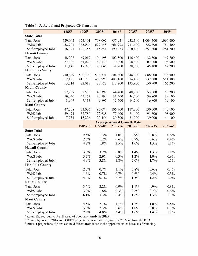
Total civilian wage and salary jobs in Hawaii are expected to increase from 666,998 in 2016 to 784,400 in 2045, an average annual growth of 0.56 percent throughout the forecast period. Total jobs (wage and salary jobs plus self-employed jobs) are projected to have a higher growth rate than that of wage and salary jobs, from 857,951 in 2016 to 1,066,000 in 2045, an average annual growth of 0.75 percent over the projection period.

The higher growth rate of projected total jobs is due to a faster growth projected for self-employed jobs than wage and salary jobs. For the period from 1985 to 2016, self-employed jobs have achieved 3.0 percent annual growth on average, while the average annual growth of wage and salary jobs for the period was 1.3 percent. As a result, the statewide share of self-employed jobs to total jobs increased from 14.4 percent in 1985 to 22.3 percent in 2016. This trend is expected to continue in the future, but at a more moderate rate than observed in the past.

Jobs in the Neighbor Islands have increased at a faster rate than in Honolulu in the past. This trend is expected to continue over the projection period, increasing the Neighbor Island’s share of statewide total jobs from 29.6 percent in 2016 to 32.6 percent in 2045. County job projections by industry are provided in Appendix Tables A-34 through A-48.

Figure 1- 6. Average Annual Growth of Total Civilian Jobs for the State

0.0%

0.5%

1.0%

1.5%

2.0%

2.5%

3.0%

3.5%

4.0%

4.5%

5.0%


10

Table 1- 5. Actual and Projected Civilian Jobs

19851 19951 20051 20162 20253 20353 20453 State Total Total Jobs 529,042 675,401 768,002 857,951 932,100 1,004,500 1,066,000 W&S Jobs 452,701 553,046 622,148 666,998 711,600 752,700 784,400 Self-employed Jobs 76,341 122,355 145,854 190,953 220,400 251,800 281,700 Hawaii County Total Jobs 48,228 69,019 94,198 102,500 116,600 132,300 147,700 W&S Jobs 37,082 51,020 68,133 70,800 78,600 87,200 95,500 Self-employed Jobs 11,146 17,999 26,065 31,700 38,000 45,100 52,200 Honolulu County Total Jobs 410,639 500,790 538,321 604,300 648,300 688,000 718,000 W&S Jobs 357,125 418,773 450,793 487,100 514,400 537,200 551,800 Self-employed Jobs 53,514 82,017 87,528 117,200 133,900 150,900 166,200 Kauai County Total Jobs 22,967 32,586 40,399 44,400 48,900 53,600 58,200 W&S Jobs 19,020 25,473 30,594 31,700 34,200 36,800 39,100 Self-employed Jobs 3,947 7,113 9,805 12,700 14,700 16,800 19,100 Maui County Total Jobs 47,208 73,006 95,084 106,700 118,300 130,600 142,100 W&S Jobs 39,474 57,780 72,628 77,400 84,400 91,600 98,000 Self-employed Jobs 7,734 15,226 22,456 29,300 33,900 39,000 44,100

Average Annual Growth Rate 1985-95 1995-05 2005-16 2016-25 2025-35 2035-45 State Total Total Jobs

2.5% 1.3% 1.0% 0.9% 0.8% 0.6%

W&S Jobs

2.0% 1.2% 0.6% 0.7% 0.6% 0.4% Self-employed Jobs

4.8% 1.8% 2.5% 1.6% 1.3% 1.1%

Hawaii County Total Jobs

3.6% 3.2% 0.8% 1.4% 1.3% 1.1%

W&S Jobs


4.9% 3.8% 1.8% 2.0% 1.7% 1.5%

Honolulu County Total Jobs

2.0% 0.7% 1.1% 0.8% 0.6% 0.4%

W&S Jobs


4.4% 0.7% 2.7% 1.5% 1.2% 1.0%

Kauai County Total Jobs

3.6% 2.2% 0.9% 1.1% 0.9% 0.8%

W&S Jobs


6.1% 3.3% 2.4% 1.6% 1.3% 1.3%

Maui County Total Jobs

4.5% 2.7% 1.1% 1.2% 1.0% 0.8%

W&S Jobs


7.0% 4.0% 2.4% 1.6% 1.4% 1.2%

1 Actual figure, source: U.S. Bureau of Economic Analysis (BEA) 2 County figures for 2016 are DBEDT projections, while state figures for 2016 are from the BEA. 3 DBEDT projections, figures can be different from those in the appendix tables because of rounding.

11

Due to multiple job holders, the number of employed has been lower than the number of jobs. In 2016, there were 664,100 civilian employed in Hawaii, which was 77.4 percent of the number of total civilian jobs. The state’s total civilian employed is projected to reach 757,000 by 2045, an annual growth of 0.45 percent and a 14.0 percent increase from the 2016 level.

Table 1- 6. Actual and Projected Civilian Employed

19851 19951 20051 20161 20252 20352 20452

State Total 452,000 552,000 608,950 664,100 694,600 728,100 757,000

Hawaii County 46,150 58,600 78,000 88,200 95,700 106,700 117,600

Honolulu County 341,150 405,850 427,000 458,000 474,000 488,500 499,500

Kauai County 20,550 25,550 31,000 34,700 36,300 39,000 41,600

Maui County 44,150 62,050 72,950 83,200 88,700 93,900 98,300


1985-95 1995-05 2005-16 2016-25 2025-35 2035-45

State Total

2.0% 1.0% 0.8% 0.5% 0.5% 0.4%

Hawaii County

2.4% 2.9% 1.1% 0.9% 1.1% 1.0%

Honolulu County

1.8% 0.5% 0.6% 0.4% 0.3% 0.2%

Kauai County

2.2% 2.0% 1.0% 0.5% 0.7% 0.6%

Maui County

3.5% 1.6% 1.2% 0.7% 0.6% 0.5% 1 Actual figure, source: Hawaii State Department of Labor & Industrial Relations 2 DBEDT projections.

4. Tourism

Visitor arrivals in Hawaii have gone through several different growth phases. Between 1960 and 1973, arrivals grew at a double-digit rate with an average annual growth rate of 18.3 percent. The growth slowed down between 1973 and 1990 with visitor arrivals growing at 5.7 percent annually before a decade long stagnation started. Visitor arrivals increased only 0.3 percent annually during 1990 to 2000. Starting in 2004, Hawaii visitor industry experienced rapid growth again, with visitor arrivals peaking in 2006 with 7.5 million visitors. Although the global economic downturn started in 2008 decreased visitor arrivals to Hawaii back to under 6.5 million in 2009, the loss was fully recovered within a few years. The number of visitors who came to Hawaii increased on average 4.7 percent per year from 2009 to 2017, marking a new record every year since 2012. In 2017, 9.26 million visitors came to Hawaii by air and including people who came by ship, 9.38 million visitors came.

The latest short-term forecasts by DBEDT (Quarterly Statistical & Economic Report: 1Q 2018) projected that the growth of visitor arrivals will slow down at 1.4-2.7 percent annually for the next 4 years. This projection for the near future is incorporated in this version of long-range projections. Long term visitor growth in Hawaii, however, will be affected not only by the

12

demand for Hawaii tourism but also the supply constraints in the state. Given the maturity of Hawaii’s tourism industry and the increasing competition from other destinations, Hawaii’s visitor arrivals are expected to grow at a slower rate into the long-term future as presented in Figure 1- 7. Detailed projection of Hawaii tourism for visitor arrival, days, daily census, expenditure and occupied visitor units are included in Appendix Table A-60 and A-61. Methodology and assumptions employed for the projections are explained in the next methodology section.

Figure 1- 7. Visitor Arrivals by Air, History and Projection

0

2

4

6

8

10

12

14

1970 1975 1980 1985 1990 1995 2000 2005 2010 2015 2020 2025 2030 2035 2040 2045

Mill

ions

Visitor Arrivals by Air

Actual ------ Projection

10.0%

6.9%

4.3%

6.8%

-0.5%1.2% 1.3%

-1.4%

4.4%2.7%

1.0% 1.0% 0.9% 0.8% 0.8%

-2.0%

0.0%

2.0%

4.0%

6.0%

8.0%

10.0%

12.0%

Avg. Annual growth rate


13

II. Hawaii Population and Economic Projection Methodology

The DBEDT 2045 projection series were produced using the Hawaii Population and Economic Projection and Simulation Model, which was developed by the Department in 1978 and refined over the years. It is an inter-industry econometric model that generates economic forecasts for the state and its four counties on an annual basis.

The 2045 Series uses the detailed population characteristics from the 2010 decennial census and 2016 vintage population estimates by the U.S. Census Bureau, 2016 job and income data from the Bureau of Economic Analysis, and the 2012 Hawaii input-output (I-O) tables as baseline data for the projection.

The model contains five blocks: final demand, income, output, employment, and population. The final demand components are either projected by a set of econometric equations or exogenously given. The statewide projected final demands are allocated to each industry using the relevant final demand vectors in the 2012 I-O table. Industrial outputs are then derived by multiplying the projected final demands by the total requirements matrix of the 2012 I-O table.

Jobs are derived by dividing each industry’s projected output by job-to-output ratio. Once jobs are projected, labor income is estimated as a function of total jobs.

The population projection is done separately using the cohort component method. However, the demographic module interacts closely with the economic module, as the demographic size and characteristics are key factors in determination of many economic variables.

For endogenous variables, regression-based analyses are conducted to capture economic relationships among the variables. To capture county-specific behavior, the variables are estimated at the county level whenever necessary data are available. When data are not available at the county level or when estimations at the county level involve excessive randomness, variables are estimated at the state level and the state-level estimates are allocated to each county using other relevant information.

With a few exceptions, variables are estimated in logarithmic forms so that the estimated coefficients represent elasticities of dependent variables with respect to the change in explanatory variables. When the estimation results show the presence of autocorrelation in error terms, AR (autoregressive) terms are added to the equations to correct the problem.

The following sections describe the demographic and economic modules of the model.

14

1. The Demographic Module

The resident population is divided into three components: military personnel, military dependents, and other civilians. The number of military personnel and their dependents stationed in Hawaii is mainly the result of national defense considerations with the state’s economic situation having little impact. In the current projections, the population of active-duty military personnel and their dependents were assumed to be exogenous using information available at the time of the projection. The projected totals were then allocated to each age and sex category using the age and sex composition of military personnel and their dependents. The age and sex composition of military personnel and their dependents were derived from the Public Use Micro Sample data of American Community Survey covering the 5-year period from 2011 to 2015.

The other civilian component of population was projected from a base population using the cohort-component method. Other civilian population at a year t is estimated as the population from the previous year, plus births minus deaths plus net migration.

CIVILIANt,k = CIVILIANt-1,k-1 + BIRTHSt - DEATHSt,k + NETMIGt,k

where CIVILIANt,k: number of other civilians at age k in year t

BIRTHSt : number of newborn babies in year t

DEATHSt,k : number of other civilians deceased at age k in year t

NETMIGt,k : number of net migrants at age k in year t

The foundation data sets used for population projections include the 2010 decennial census data, 2016 vintage population estimates by the U.S. Census Bureau, and birth and death data collected by the Hawaii Department of Health.

Projection of the population is based on a complex set of assumptions about fertility and mortality. These assumptions play a key role in determining the size of natural population increase and age structure of the population in the future. Methodologies used in estimating current levels of fertility and mortality rates, and assumptions about their future levels are explained in detail below.

Fertility Rates

The age-specific fertility rates were calculated by dividing the number of births by the number of female population in each age category. An age-specific fertility rate indicates the probability that a woman of childbearing age will give birth in a given year. Multiplied by the number of females of childbearing age, fertility rates estimate the number of births that will take place in a given year.

15

The detailed data on historical births in Hawaii were obtained from the Hawaii State Department of Health. The data contained information on each individual birth compiled by sex of baby, age of mother and the county of residence. Since the size of military dependent population was assumed to be determined by the number of armed forces stationed in Hawaii, the cohort component method was applied only to the other civilian population in the projection. The data from the Hawaii State Department of Health included some information about military status of the baby’s parents. However, the information was not detailed enough to effectively separate the births in military families from the births in other civilian population. Thus, we estimated the age-specific fertility rates of whole resident population and used them to project the births in other civilian population assuming that fertility rates of military families were not much different from fertility rates of other civilian population once mother’s age was controlled. To mitigate random fluctuation in estimates due to small sample size, data for three years from 2013 to 2015 were averaged to produce 2014 estimates of age-specific fertility rates for each county (Appendix Tables A-22 through A-26).

The next step was to adjust the calculated 2014 fertility rates for the likely change in the future fertility rates. Fertility rates change over time because of changes in age and ethnicity composition, maternity patterns, socio-economic factors, and changes in policies that may affect the cost of bearing and raising children. Fertility rates in most developed countries have declined sharply for many decades since the end of baby boom years. In the U.S., the downward trend continued until mid- 1970s. Although fertility rates fluctuated since then, fertility rates in the U.S. in 1990s and 2000s remained higher than those in 1970s and 1980s in general.

Fertility rate in Hawaii has shown similar trend albeit it has been higher than the U.S. average and has shown more fluctuations. Total fertility rate, that measures the hypothetical number of children who would be born to a woman in her life time when the current age-specific fertility rates are applied, increased from 2.01 in 1997 to 2.33 in 2008 in Hawaii. However, as observed in the nationwide trend, fertility rate in Hawaii declined during the recession starting from 2008. Interestingly, the decline in fertility rate continued even after the economy recovered from the recession, implying that the economic hardship was not the only cause of the decline. Total fertility rate of Hawaii was estimated at 1.947 for 2016.1

The key question to be answered is whether the decline is a permanent trend or a temporary phenomenon due to delay in marriage and first birth. If the decline was due to just delaying marriage and childbirth, the decline may be recovered, at least partially if not all, in the future. Figure 2- 2 below compares the number of births in Hawaii per 1,000 women in each 5-year childbearing age group in 2008 and 2016. A decline in fertility rate was broadly observed for women ages under 35, and the decline was especially big for teenagers and women in low 20s.

1 National Vital Statistics Report, Births: Final Data for 2016, January 2018, National Center for Health Statistics, Centers for Disease Control and Prevention

16

This trend is similar to the nationwide trend except that the nationwide trend showed an increase in fertility rates in the 30-34 age group.

Figure 2- 1. Trend of Fertility Rates in Hawaii and the U.S.

Figure 2- 2. Fertility Rates in Hawaii by the Age of Mother, 2008 vs. 2016

Source: Births: Final Data for 2008, 2016, National Center for Health Statistics, Centers for Disease Control and Prevention

The most recent national population projections by the U.S. Census Bureau, released in 2014, made a separate projection of total fertility rate for each of five groups defined by mother’s country of birth. In that version of national projections, fertility rates of all foreign-born population other than Non-Hispanic API (Asian and Pacific Islander) were projected to decline while fertility rates of natives and foreign-born API were projected to slightly increase over its

Hawaii

U.S. average

1.0

1.2

1.4

1.6

1.8

2.0

2.2

2.4

2.6

2.8

3.0

1990

1991

1992

1993

1994

1995

1996

1997

1998

1999

2000

2001

2002

2003

2004

2005

2006

2007

2008

2009

2010

2011

2012

2013

2014

2015

2016

Total Fertility Rate

0

20

40

60

80

100

120

140

15-19 20-24 25-29 30-34 35-39 40-44 45-49

Age of mother

Number of births per 1,000 women in the age group

2008 2016 Total fertility rate

2008: 2.33

2016: 1.94

17

projection period ending in 2060. Combined with its population projection of the five groups, total fertility rate of total U.S. population was projected to be 1.86 in 2060, almost no change from 1.87 in 2014.2

In this version of population projection, we assumed that total fertility rate in Hawaii will increase slightly to 2.03 by 2020 and stay unchanged during the rest of the projection period.

Table 2- 1. Total Fertility Rate: History and Projection

Year 1990 1995 2000 2005 2010 2016 2020-2045*

Total fertility rate 2.33 2.19 2.14 2.28 2.15 1.94 2.03 *DBEDT projections

Life Tables and Survival Rates

Life tables for the resident population of four counties were developed using the same life table methodology as used for the U.S. national life tables with a few modifications.3

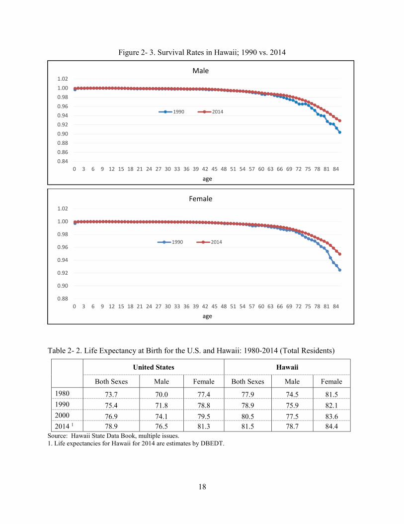
Compared to fertility rates, the future direction of changes in mortality rates is less controversial. With better health services and increased affluence, mortality rates have generally decreased over time and will continue to decrease (Figure 2- 3). The question is to what degree and in what pattern the mortality rates would decrease in the future. In this projection, age- and sex-specific mortality rates were adjusted in the following manner. Firstly, target life expectancies at birth for the four counties in Hawaii were developed using target life expectancy for the nation developed by the Census Bureau as references. The latest national population projection by the U.S. Census Bureau, published in 2014, projected mortality rates and life expectancies for three race groups. It projected that life expectancy at birth for Non-Hispanic White and API group will increase gradually from 77.4 years for the male population and 81.8 years for the female population in 2014 to 84.6 years for the male population and 87.5 years for the female population in 2060.4 Based on a review of historical relationship between life expectancy in Hawaii and those of the U.S., target life expectancies for the four counties in Hawaii in 2045 were developed as presented in Table 2- 3.

2 Methodology, Assumptions, and Inputs for the 2014 National Projections, December 2014, U.S. Census Bureau 3 “United States Life Tables, 2014”, National Vital Statistics Reports, Center for Disease Control and Prevention, August 2017. Palmore, J. and R.Gardner, Measuring Mortality, Fertility, and Natural Increase, East-West Center, Honolulu, 1994. 4 Methodology and Assumptions for the Population Projections of the United states: 1999 to 2100, Population Division Working Paper N0.38, Population Division, U.S. Census Bureau, January 2000.

18

Figure 2- 3. Survival Rates in Hawaii; 1990 vs. 2014

Table 2- 2. Life Expectancy at Birth for the U.S. and Hawaii: 1980-2014 (Total Residents)

United States Hawaii

Both Sexes Male Female Both Sexes Male Female

1980 73.7 70.0 77.4 77.9 74.5 81.5 1990 75.4 71.8 78.8 78.9 75.9 82.1 2000 76.9 74.1 79.5 80.5 77.5 83.6 2014 1 78.9 76.5 81.3 81.5 78.7 84.4

Source: Hawaii State Data Book, multiple issues. 1. Life expectancies for Hawaii for 2014 are estimates by DBEDT.

0.84

0.86

0.88

0.90

0.92

0.94

0.96

0.98

1.00

1.02

0 3 6 9 12 15 18 21 24 27 30 33 36 39 42 45 48 51 54 57 60 63 66 69 72 75 78 81 84

age

Male

1990 2014

0.88

0.90

0.92

0.94

0.96

0.98

1.00

1.02

0 3 6 9 12 15 18 21 24 27 30 33 36 39 42 45 48 51 54 57 60 63 66 69 72 75 78 81 84

age

Female

1990 2014

19

Table 2- 3. Projected Life Expectancy at Birth for Hawaii: 2014 and 2045 (Other Civilian)

Life Expectancy in 20141 Projected Life Expectancy in 20452

Male Female Male Female

State of Hawaii 78.7 84.4 83.8 88.5

Hawaii County 77.2 83.4 82.3 87.4

Honolulu County 79.0 84.6 84.1 88.7

Kauai County 79.4 84.4 84.5 88.5

Maui County 78.2 84.1 83.3 88.2 1 DBEDT Estimates. 2 DBEDT Projections.

The next step involved adjusting mortality rates to meet the target life expectancies. To develop the pattern of mortality decline in the future, the Census Bureau collected expert opinions regarding how much faster the mortality rates of some age groups will decline in the future relative to the others. They divided the population into three age groups: under 15, between 15 and 65, and over 65. Its survey found that “average annual rate of mortality decline” experienced by the age group under 15 years will be 2.1 times higher than that of the age group over 65 years until 2020 and 1.6 times higher for the year after 2020. For the age group between 15 to 64 years, it will be 1.3 times higher than that of the age group over 65 years until 2020 and 1.2 times higher for the year after 2020. 5

In this projection, the same rates of mortality decline as developed by the Census Bureau were assumed with one modification. The age group over 65 years was further divided into two groups: age group between 65 and 84 and age group over 85. This modification was introduced with the notion that mortality rates for extremely high ages tended to be underestimated in Hawaii. Underestimation of mortality and overestimation of population at extremely high ages have been reported by many demographers.6 In order to reduce this potential exaggeration of older population, it was assumed that mortality rates of the age group over 85 years would decrease at a rate lower than that of the age group between 65 to 84 years throughout the projection period.

Using these assumptions, life tables for the projection period were constructed to project annual population and deaths of other civilians for each county.

5 See the same reference as in the footnote 4. 6 Wilmoth, J.R., “Are Mortality Rates Falling at Extremely High Ages: An Investigation Based on a Model Proposed by Coale and Kisker”, Population Studies, Vol.49. No.2, July 1995, pp281-295.

20

Net Migration

Migration plays an important role in population growth. Not only the initial number of people who migrated to the area, but their descendants contribute to population growth. It also impacts age structure of the population. Migrants have a younger age structure in general. Four charts in Figure 2- 4 compares age structures of in- and out- migrants to/from Hawaii with that of total population based on 2011-2015 American Community Survey data. It shows that both in- and out-migrants had much younger age structure, with a high concentration especially in the 20-35 age range. With a younger age structure, migrants help to augment working-age population in the economy and it also slows down aging of population to a certain extent.

Figure 2- 4. Age Distribution of Migrants

1. DBEDT calculation based on the 2016 vintage population estimate by the US Census Bureau 2. DBEDT estimation using 2015 5-year American Community Survey, Public Use Micro Sample data

The number to be added to existing population for population projection is net migration that subtracts out-migration from in-migration. Migration data are available from a few sources. Intercensal population estimates by the U.S. Census Bureau includes annual estimates of total domestic and international net migration. However, intercensal population estimates were sometimes turned out to be considerably off from actual figures when the decennial census came out, mainly due to inaccurate estimation of migration. Total number of migrants can also be

0% 5% 10% 15% 20%

0-45-9

10-1415-1920-2425-2930-3435-3940-4445-4950-5455-5960-6465-6970-7475-7980-84

85 & over

Residents in Hawaii 1

age

Share of total

0% 10% 20%

International In-migrants 2

Share of total

0% 10% 20%

Domestic In-migrants 2

Share of total0% 10% 20%

Domestic Out-migrants 2

Share of total

21

estimated based on American Community Survey (ACS). Although ACS provides useful information about the characteristics of migrants, the estimates of total migrants based on ACS were quite different from the estimates from the intercensal population estimates. Another widely used method of estimating migration is to estimate migration over ten-year period between two decennial censuses as the difference between population change and natural increase during the period. Table 2- 4 presents the average annual net-migration to Hawaii from 1980 to 2010 estimated using this residual method. On average, about 5,100 migrants were added every year to other civilian population in Hawaii during the 1980-2010 period. If we incorporate the migration estimates from the 2017 intercensal population estimates by the U.S. Census Bureau, long-term averages of annual net-migration to Hawaii from 1980 to 2017 was about 4,800 per year. The 1980-2017 period includes both recession and boom cycles of the economy while it excludes the high growth period before 1980. The size of migration will vary by year along with business cycles over the projection period. However, following the long-term trend that the state experienced since 1980, the state is assumed to have 4,800 net-migrants every year during the projection period.

Table 2- 4. Estimation and Projection of Net-Migration

Resident Population Other Civilian Population

Population Change

Natural increase

Estimated Migration

Population Change

Natural increase

Estimated Migration

1980-1990 14,350 13,030 1,320 14,780 11,020 3,750

1990-2000 10,330 11,210 -880 13,030 9,380 3,650

2000-2010 14,880 9,320 5,560 15,500 7,590 7,900

Projected net-migration for the projection period: 4,800 for Other Civilian Population

Historically, international migration and domestic migration have shown very different trends. Domestic migration fluctuated a great deal even within a same stage of business cycles while the size of international migration has been relatively stable in the past. In this version of the projection, international net migration was assumed to remain constant at 7,500, its average value of the past 7 years. The size of net domestic migration during the projection period was determined by subtracting international net migration from total net-migration.

The projected international and domestic net-migration statewide were then allocated to each county by single age-sex category. Each county’s share and the sex age distribution of migrants were estimated using the Public Use Micro Sample data from the 2015 five-year American Community Survey (ACS).

22

2. The Economic Module

Projection of GDP and Final Demand

Gross Domestic Product (GDP) for states is the state equivalent of GDP for a nation. Two approaches can be used to estimate GDP for a state: the income approach and the expenditure approach. GDP estimates published by the U.S. Bureau of Economic Analysis (BEA) are measured using the income approach as the summation of the factor income earned and costs of production. We estimated GDP using the expenditure approach as follows;

GDP = C + I + G + ( X – M )

where C : Personal consumption expenditures I : Private investment G : Government spending, including government investment X : Exports M : Imports

Conceptually, the two approaches should yield the same estimates since they are basically two different methods for measuring the state’s overall economic activity. However, due to many practical details involved in calculating nominal and real GDP, the estimates of GDP included in the projections need to be compared to the BEA’s estimates of GDP with caution.

Each component of GDP can be divided into many sub-components for an effective estimation. Exports were divided into tourism export and non-tourism exports. Government spending was defined in terms of three components: state and local government spending, federal military spending, and federal civilian spending. Due to lack of data at the county level, most components of final demand were projected at state level.

In all estimation equations presented in this report, the subscript ‘t’ indicates year while ‘i’ indicates industry.

Personal Consumption Expenditures

The annual estimates of personal consumption expenditures (PCEs) for the State of Hawaii were no longer available after 2000 when DBEDT decided to use BEA’s estimates of GDP by State instead of estimating on its own. From then on, PCEs of Hawaii were estimated only once every few years as part of the construction of the Hawaii I-O tables. Historically, however, personal consumption had shown a relatively stable relationship with income. Assuming the continuation of the relationship over time, PCEs were estimated as a function of disposable personal income (DPI) as follows;

23

ln(PCEs)t,state =0 + 1 • ln(DPI)t, state + AR(1) The first order autoregressive term- AR(1) - was included to correct the autocorrelation in error.

Private Investment

Determining the size of the capital stock of an economy, investment is a key element of long-term economic growth. In spite of this, forecasting future levels of investment is not an easy task due to its severe volatility and cyclical behavior. A number of different model specifications were examined using data from many different sources. At the end of numerous econometric exercises, the following specification was adopted.

Private investment (PIV) was modeled as a function of the demand for houses (DHOUSE), unemployment rate (UNEMPRT), and the previous level of PIV. The unemployment rate was included to account for the sensitivity of the private investment to short-term fluctuations of the economy. Demand for houses was calculated by dividing total population with average household size for that year.

PIVt,state =0 + 1 • UNEMPRTt,state + 2 • DHOUSEt,state + 3 • PIVt-1,state

statet,

statet,statet, Size Household

PopulationDHOUSE

Government Spending

The projection of state and local government spending (SLGS) was projected as a function of personal income (PI) as follows.

ln(SLGS)t,state =0 + 1 • ln(PI)t, state + AR(1)

Federal government spending was divided into two categories: military spending and civilian spending. Federal government civilian spending (FGCS) was estimated using an econometric model, while exogenously determined growth rates were applied to project military spending. Similar to state and local government spending, federal government civilian spending was assumed to depend on statewide personal income while federal government military spending was assumed to grow at about 1 percent annually in real terms over the forecast period.

ln(FGCS)t,state =0 + 1 • ln(PI)t, state + AR(1)

24

Exports

Exports consist of the commodities and services that are sold to people and businesses outside the State of Hawaii. If constraints in local production capacity are not considered, the level of exports would depend solely on factors outside the economy. For this reason, future levels of exports were either exogenously given or projected using a separate model.

Exports consist of tourism exports (visitor expenditures) and non-tourism exports. A detailed description of the methodology used for the projection of visitor expenditures is presented in the tourism section.

With little information on factors affecting non-tourism exports, they were modeled to be determined by the size of output. That is, exports for each industry were calculated assuming that the proportions of output to be exported in total output would remain constant at the levels in the 2012 I-O table.

Imports

The 2012 I-O tables contain information on proportions of inputs imported from outside the Hawaii economy for each industry and final demand sectors in that year. It was assumed that these proportions would remain constant over the projection period. Total imports were then estimated by multiplying the projected outputs and final demands by these import coefficients.

Projections of Output

Historical data on industrial outputs in Hawaii are not available on an annual basis. The U.S. Census Bureau publishes output data by industry at five-year intervals with a three- year lag. The 2012 I-O tables of Hawaii were updated based on the 2012 Economic Census, which was the most recent release of output data by the Census Bureau at the time of the construction of the I-O tables.

The 2012 Hawaii I-O tables are available in two versions of industry aggregations. A detailed table includes 68 industry sectors, while a condensed table has 20 industry sectors. Industry classification in this projection series is consistent with the classification in the condensed version of the 2012 I-O tables. A detailed description of the 2012 Hawaii I-O tables is available on the DBEBT’s web site at http://dbedt.hawaii.gov/economic/reports_studies/2012-io/.

The I-O tables include detailed information on flows of goods and services among the final demand and the producing sectors in the economy. Annual outputs for each industry were projected by applying the final demand-output relationships in the 2012 Hawaii I-O tables to the annually-projected final demands. To estimate final demand for an industry, each component of projected final demands was distributed among industries using the final demand coefficients derived from the I-O table. Total final demand for an industry was then estimated by summing up the individual components. The industry outputs were estimated using industries’ projected

25

final demands and the total requirement matrix from the 2012 I-O table. These projected outputs, in turn, formed the basis for projecting job counts by industry.

Projections of Jobs

Jobs data reported in this projection series are consistent with the BEA job data in definition and coverage with the exception that military jobs were subtracted from the BEA jobs data to calculate civilian jobs.

The projection of jobs involves two types of jobs: wage and salary jobs and self-employed jobs. In this projection, total jobs (wage and salary jobs plus self-employed jobs) were first projected for each industry using the ratios of total jobs to output, and then the wage and salary jobs and self-employed jobs were estimated based on their relationships to total jobs.

Total jobs (TJOB) for each industry at the state level were projected by multiplying corresponding outputs with industry specific total jobs-to-output ratios. As a result of productivity increase, more output per job and thus, fewer new jobs are required to increase output by a given amount. The job-to-output ratios were derived from the 2012 I-O tables and adjusted from the 2012 levels to reflect this advancement in production technology. Because of unavailability of annual output data, estimates of labor productivity growth were developed using the historical ratios of jobs and real GDP for each industry. The projected statewide total jobs by industry were then allocated to four counties based on historical trends.

statei, t,statei, t,state i, t, )OUTPUT

TJOB(OUTPUTTJOB

i state i, 1,-tstate i, t, Factorty Productivi )OUTPUT

TJOB()

OUTPUT

TJOB(

Wage and salary jobs (WSJOB) were projected using the projections of total jobs, and industry and county specific ratios of the wage and salary jobs to the total jobs. The ratios of wage and salary jobs to total jobs were also adjusted to account for the observed trend of the increasing share of self-employed jobs. The statewide share of self-employed jobs out of total jobs increased from 14.4 percent in 1985 to 22.3 percent in 2016. The increasing trend is found in all four counties, albeit not to the same degree.

county i, t,countyi, t,countyi, t, )TJOB

WSJOB(TJOBWSJOB

countycounty i, 1,-tcounty i, t, Factor Changing Annual )TJOB

WSJOB()

TJOB

WSJOB(

26

Self-employed jobs (SEJOB) for each industry for each county were then calculated as the residual.

SEJOB =TJOB - WSJOB

Projections of Employment

Employment can be defined in two ways. One is person-based and the other is position-based. In general, employment data that are published with labor force and unemployment data are based on household surveys, and are therefore, person-based. In this case, employment is defined as the number of people who are employed in a given period regardless of whether the person is working full-time or part-time.

On the other hand, the position-based employment is defined as the number of positions, full-time or part-time, in a given period. In this report, the term “Employment (or Employed)” is used to denote the person-based employment, and “Jobs” is used to denote the position-based employment.

Typically, jobs exceed employed because of multiple-job holders. If a person holds two part-time positions, the person would be counted once in the employment data but twice in the jobs data.

EMPLOYED was estimated as a function of total jobs. Although the ratio of employed to total jobs has shown decreasing pattern in all four counties, the decreasing patterns are quite different across counties. For this reason, EMPLOYED was estimated for each county separately.

ln(EMPLOYEDt, county) = 0 + 1 • ln(TJOBt, county ) + AR(1)

Projections of Income

Personal income (PI) was projected in terms of four components: labor income, transfer payments, property income (dividends, interests and rent), and contributions for government insurance. Each of these components was projected as described below, and the following formula produces the projections of personal income;

Personal Income = Labor Income + Transfer Payment + Property Income

– Contributions for Government Social Insurance

Labor Income

Labor income (LINC) includes wages and salaries, supplements to wages and salaries, and proprietors’ income. It was projected for each county as a function of total jobs in the county.

27

ln(LINC)t, county = 0 + 1 • ln(TJOB)t, county + AR(1)

Transfer Payments

Transfer payments (TRANS) include retirement and disability insurance, Medicare and other medical benefits, unemployment insurance, and other federal assistance payments. Thus, it was modeled to depend on the size of population aged 65 year and over (POP65) and unemployment rate (UNEMPRT).

ln(TRANS)t, county = 0 + 1 • ln(POP65)t, county + 2 • UNEMPRTt, county + AR(1)

Property Income

Property income (DIR) includes dividend income, personal interest income, and rental income. Many factors, such as interest rate, stock price, and housing price, will affect the future size of property income. Due to the large uncertainty involved with these variables, however, property income of each county was estimated based on its historical relations to personal income.

ln(DIR)t,county = 0 + 1 • ln(PI)t, county + AR(1)

Contributions for Government Social Insurance

Contributions for government social insurance (CGI) consist of employer contributions for government social insurance and employee and self-employed contributions for government social insurance. It was estimated as a function of labor income.

ln(CGI)t, county = 0 + 1 • ln(LINC)t, county + AR(1)

Disposable Income

Subtracting personal tax from the projected personal income gives disposable income.

Disposable Income = Personal Income – Personal Tax

Personal tax is estimated as a function of personal income. Since total personal tax is more or less determined as a proportion of aggregated income, personal tax was estimated in raw value rather than in logarithm. In this way, personal tax would grow about at a same rate as personal income.

PTAX t, state = 0 + 1 • PIt, state + AR(1)

Tourism Projections

Tourism projections underlying DBEDT 2045 series were developed using both econometric modeling and relationship analysis. Visitor arrival, days, and expenditure, statewide and by

28

county, were projected in the following sequences using the assumption presented in the Table 2-6 through Table 2-8.

Visitor Arrival Projections

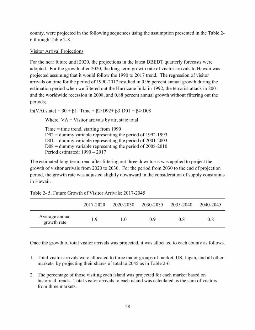
For the near future until 2020, the projections in the latest DBEDT quarterly forecasts were adopted. For the growth after 2020, the long-term growth rate of visitor arrivals to Hawaii was projected assuming that it would follow the 1990 to 2017 trend. The regression of visitor arrivals on time for the period of 1990-2017 resulted in 0.96 percent annual growth during the estimation period when we filtered out the Hurricane Iniki in 1992, the terrorist attack in 2001 and the worldwide recession in 2008, and 0.88 percent annual growth without filtering out the periods;

ln(VAt,state) = β0 + β1 ·Time + β2·D92+ β3·D01 + β4·D08

Where: VA = Visitor arrivals by air, state total

Time = time trend, starting from 1990 D92 = dummy variable representing the period of 1992-1993 D01 = dummy variable representing the period of 2001-2003 D08 = dummy variable representing the period of 2008-2010 Period estimated: 1990 – 2017

The estimated long-term trend after filtering out three downturns was applied to project the growth of visitor arrivals from 2020 to 2030. For the period from 2030 to the end of projection period, the growth rate was adjusted slightly downward in the consideration of supply constraints in Hawaii.

Table 2- 5. Future Growth of Visitor Arrivals: 2017-2045

2017-2020 2020-2030 2030-2035 2035-2040 2040-2045

Average annual growth rate

1.9 1.0 0.9 0.8 0.8

Once the growth of total visitor arrivals was projected, it was allocated to each county as follows.

1. Total visitor arrivals were allocated to three major groups of market, US, Japan, and all other

markets, by projecting their shares of total to 2045 as in Table 2-6.

2. The percentage of those visiting each island was projected for each market based on historical trends. Total visitor arrivals to each island was calculated as the sum of visitors from three markets.

29

Table 2- 6. Assumptions Employed for the Projections of Visitor Arrivals1

1990 2000 2010 2017 2030 2045

Share of each market in total visitors (%)

US 61.8 59.7 65.6 63.1 60.8 58.0 Japan 22.2 26.2 17.9 16.9 16.4 16.0 All other market 16.0 14.2 16.5 19.9 22.8 26.0

Percentage of visiting each island among total visitors (%)

Hawaii 17.5 18.2 18.5 19.0 20.0 21.1 Honolulu 78.3 67.9 61.8 61.3 58.6 55.8 Kauai 19.1 15.5 13.8 13.8 13.9 14.0 Maui 35.3 33.2 30.7 30.1 30.8 31.6

1. Include visitors who arrive by air only

Visitor Days and Daily Visitor Census

Visitor days and daily visitor census were projected by the following sequence and assumptions:

1. LOS (length of stay) was projected for each of three markets for the projection period. 2. Visitor days of each market was calculated as the product of visitor arrivals from the market

and LOS of the market. 3. Statewide visitor days were projected as the sum of projected visitor days of three markets. 4. Visitor days by county were projected as the product of “statewide visitor days” and “county

share of visitor days”. County shares of visitor days were developed based on historical trends.

5. Average daily visitor census = visitor days/ 365 or 366 for leap years

Table 2- 7. Assumptions Employed for the Projections of Visitor Days1

1990 2000 2010 2017 2030 2045

Length of stay (days)

US 9.4 10.0 9.9 9.4 9.5 9.5 Japan 5.9 5.6 5.9 5.9 5.8 5.8 All other market 8.0 10.1 11.3 10.3 10.0 10.0

County share of visitor days (days)

Hawaii 10.8 12.9 14.0 14.7 15.6 16.7

Honolulu 53.6 50.4 48.4 46.2 43.7 40.8 Kauai 11.2 10.7 11.0 11.4 11.7 12.0 Maui 24.4 26.0 26.6 27.7 29.0 30.5


30

Visitor Expenditures

Visitor expenditure by visitors who arrived by air, and total expenditure were projected by the following sequence and assumptions:

1. PPPD (per person per day spending) was projected for each of three markets: PPPD increased 1.8 percent, 0.3 percent, and 3.3 percent annually on average from 2001 to 2017 for US, Japan, and all other markets respectively. This growth reflects not only the increase in price level but also the change in spending pattern, such as less shopping, and the change in market composition in the case of all other markets. For the future, we project that PPPD will increase 1.8 percent, 1.5 percent, and 2.0 percent annually for US, Japan, and all other market respectively, assuming no significant change in spending pattern and market composition during the projection period.

2. Visitor expenditure of each market was calculated as the product of visitor days and PPPD of the market.

3. Statewide visitor expenditure by visitors who arrived by air was projected as the sum of the projected visitor expenditure of three markets.

4. Visitor expenditure by county were projected as the product of “statewide visitor expenditure” and “county share of visitor expenditure”. County shares of visitor expenditure were developed based on historical trends.

5. Once the expenditures by air visitors were projected, total visitor expenditures were projected by adding supplemental business expenditure and the expenditure by visitors who arrived by ship.

Total Visitor Expenditure = Air visitor expenditure + Supplemental business expenditure + Cruise visitor expenditure

Table 2- 8. Assumptions Employed for the Projections of Visitor Expenditures1

2001 2010 2017 2030 2045

PPPD (in current dollar)

US 142.7 153.5 189.7 239.0 312.3 Japan 227.0 261.1 237.9 296.8 371.1 All other market 126.9 169.9 213.7 276.6 372.2

County share of visitor expenditure (%)

Hawaii 12.5 13.4 14.2 15.2

Honolulu 50.8 46.4 43.9 41.0 Kauai 10.3 10.6 10.9 11.2 Maui 26.5 29.6 31.0 32.7


2QRWNCVKQP CPF 'EQPQOKE 2TQLGEVKQPU HQT VJG 5VCVG … · l 7deoh ri &rqwhqwv /lvw ri 7deohv ll

Documents

Transcript of 2QRWNCVKQP CPF 'EQPQOKE 2TQLGEVKQPU HQT VJG 5VCVG … · l 7deoh ri &rqwhqwv /lvw ri 7deohv ll