University of Wisconsin-Madison 2"k 7fi'

Institute for Research on Poverty Discussion Papers

Peter A. Streufert

THE EFFECT OF UNDERCLASS SOCIAL ISOLATION ON SCHOOLING CHOICE

Institute for Research on Poverty Discussion Paper no. 954-9 1

The Effect of Underclass Social Isolation on Schooling Choice

Peter A. Streufert Department of Economics and

Institute for Research on Poverty University of Wisconsin-Madison

August 199 1

I thank Wayne Sigelko for his research assistance, and the Institute for Research on Poverty for its financial support.

Abstract

I model underclass social isolation as the loss of high-income role models, and study the

plausible conjecture that this truncation depresses schooling choice. Although the conjecture stands in

calibrated simulations, it fails at many other parameter values: truncation might not decrease a

youth's estimate of incremental postschool income, and it always decreases a youth's estimate of

forgone income. I also show that the introduction of untruncated role models during college can

polarize underclass youth, and that welfare depresses schooling choice through a distinct and

reinforcing channel. Numerous simulations exhibit the severity of these effects, and suggestions for

empirical testing are offered.

THE EFFECT OF UNDERCLASS SOCIAL ISOLATION ON SCHOOLING CHOICE

1. Introduction

In this paper, I formally analyze one central thesis of Wilson's (1987)

book The Truly Disadvantaged, namely, the thesis that the social isolation of

the underclass causes underclass youth to underestimate the effect of schooling

on income, and consequently, to choose too little schooling.

When he states this thesis most precisely (pp. 56-58), Wilson argues that

"a perceptive ghetto youngster in a neighborhood that includes a good number of

working and professional families . . . can see a connection between education

and meaningful employment." Yet, "in a neighborhood with a paucity of regular-

ly employed families . . . the relationship between schooling and postschool

employment takes on a different meaning." This results in "a shockingly high

degree of educational retardation."

I begin my work by modeling how role models shape a youth's perception of

the relationship between schooling and income. A role model is taken to be a

single observation of the schooling and income of an adult worker in the labor

force, and many such observations enable a youth to (nonparametrically) regress

schooling on income. Thus a youth's information-gathering process resembles a

labor economist's estimation of the earnings function. If the role models that

a youth observes are representative of the labor force, then the youth will

choose an efficient amount of schooling as a consequence of utility maximiza-

tion. Section 2 defines schooling choice in this ideal "benchmark" model,

Theorem 1 provides a useful marginal characterization of this choice, and

Simulation 1 calibrates the benchmark model to fit Mincer's earnings function

and the schooling distribution of the U.S. labor force.

I then model underclass social isolation as the elimination of high-income

observations at each level of schooling. That is, I assume that an underclass

youth observes a sample of role models that is truncated from above. Wilson's

thesis suggests that the resulting bias in the regression unambiguously de-

presses schooling choice. Yet Section 3 demonstrates that this is not a logi-

cal necessity for two substantive reasons.

First, if Wilson's conjecture stands, it stands because social isolation

reduces the perceived increment to postschool income that would result from an

additional year of schooling. In other words, the thesis hinges on the idea

that truncation reduces the slope of the regression. But truncation doesn't

always reduce the slope. Counterexample 1 exhibits a very plausible instance

in which the slope steadily increases with social isolation.

Second, social isolation inevitably decreases the level of the regression.

This serves to increase, rather than decrease schooling by making a youth

underestimate the income she forgoes in attending another year of school. Thus

social isolation depresses schooling choice only if (1) it leads to a decrease

rather than an increase in the perceived incremental postschool income result-

ing from another year of schooling, and (2) the magnitude of this decrease is

sufficiently great to overcome the underestimation of forgone income. Thus,

the consequences of social isolation are quite ambiguous theoretically.

On the other hand, Simulation 2 suggests that Wilson's thesis has con-

siderable empirical relevance in spite of its theoretical ambiguity. For

instance, a youth who would have completed high school in Simulation 1's cali-

brated benchmark model only completes eighth grade in Simulation 2's model of

social isolation. This precipitous drop in schooling choice results from the

lack of any role models earning more than 16 thousand dollars per year.

In a nutshell, an economist would say that representative role models are

a "neighborhood" public good. Alternatively, a sociologist might rejoice in

hearing an economist argue that a "rational" individual's schooling choice

depends critically on that individual's social environment.

Section 4 extends the model by allowing a youth's collection of role

models to change as she proceeds through school. For instance, Simulation 3

assumes that an underclass youth's social isolation is lifted when and if she

enters college. Such changing role models can split underclass youth into two

disparate groups: one whose schooling is stunted by underclass social isola-

tion, and another that is ultimately unaffected by its underclass origins.

This accords well with empirical studies suggesting that the income distribu-

tion of American blacks is becoming increasingly polarized.

Finally, Section 5 further extends the model to incorporate the effects of

welfare on schooling choice. While social isolation truncates role models from

above, welfare censors role models from below. In contrast to social isola-

tion, welfare unambiguously reduces incremental postschool income (i.e., the

slope of the regression) and increases forgone income (i.e., the level of the

regression). It thereby unambiguously depresses schooling choice (Theorem 2).

Simulations 4 and 5 show that social isolation and welfare are very likely to

depress schooling choice through distinct and reinforcing channels. One squee-

zes the regression from above, the other squeezes from below, and the effect of

a distortion on one side is exacerbated by a distortion on the other.

Section 6 tabulates about 30 simulations which attest to the severity of

the effects brought about by social isolation and welfare. Section 7 discusses

the scant empirical evidence that can be linked to the model and makes several

suggestions for further empirical research. One key suggestion is that re-

searchers question how well mean neighborhood income correlates with social

isolation.

Finally, I make two comments about my methodology. First, my stylized

mathematical model makes many implicit and explicit assumptions in order to

derive sharp statements about the effect of social isolation on schooling

choice. These assumptions are discussed in some detail in Section 2.3. Sec-

ond, my simulations have been generated numerically by thoroughly documented

GAUSS programs which I myself have written and tested. I will be very happy to

provide the reader with a diskette at no cost.

4

2. Benchmark Model

2.1. Theory

Imagine that a young person must choose a level of schooling s from the

15-element set S = (5,6, . . . 19). Let s = 5 mean that she drops out after the

fifth grade, and let s = 19 mean that she completes high school (i.e., twelfth

grade), four years of college, plus three years of postgraduate training.

One key factor in her decision is the effect that s will have upon her

future annual income y. For simplicity, I ignore nonwage income (so that

"incomen and "earnings" are synonymous) and I assume that annual income y is

constant throughout her working career. The actual relationship between s and

y is given by the random function F = (F(S))~€~ E F', where F is the set of all

cumulative distribution functions which have nonnegative support, have a finite

mean, and assume a positive value everywhere but zero. Thus for every school-

ing s, F(s) is a c.d.f. over incomes y, and F(s)(y) is the conditional proba-

bility that a person with schooling s will have an income less than or equal to

Y.

Imagine that a young person learns about F by observing role models in the

labor force. Formally, each role model is taken to be a single observation of

schooling s and income y. Thus, for every s, the collection of role models

with schooling s constitutes a sample from the population described by F(s).

As elucidated by Manski ((1990), Section 3.1), this mathematical concept of

role models accords with the sociological concept of role models, and a collec-

tion (i.e., sample) of such role models accords with the sociological concept

of a reference group.

For simplicity, I assume asymptotic sampling. That is, I assume that for

every s, the young person learns the entire c.d.f. rather than needing to draw

statistical inferences from a finite sample. Thus, at every s, the sample

mean income and the population mean income coincide at E[F](s), where the

expectation operator E: sS + RS is defined by

and is the set of all cumulative distribution functions having nonnegative

support and finite mean. The function E[F] is a perfect nonparametric regres-

sion of income on schooling. [The second of the above integrals is equal to

the first by Mood, Graybill, and Boes ((1974), p. 65); and F 5 F since F also

requires that the cumulative distribution function assumes a positive value

everywhere but zero (I will need the generality of to accommodate C's range

in Section 5).]

Let b E (0,l) and 8 E R be a person's discount factor and taste for at-

tending school, respectively. Both are preference parameters. The parameter 6

is familiar, and the simulations will assume that all individuals share the

same 6. The parameter 8 is new. It may be regarded as the utility of attend-

ing a year of school, measured in units of annual income. Thus it decreases

with tuition and increases with financial aid and the pleasure one takes in

learning and in the classroom environment. I assume that a person knows her 8

from birth and that 8 is constant over time. The simulations will assume that

different persons have different 8's.

Given these preference parameters and the agent's knowledge of the actual

relationship between schooling and income, I suppose that the agent chooses

schooling (s) to maximize the utility function defined by

The index a denotes age minus six (i.e., age measured by one's grade in

school). Thus a = 59 coincides with retirement at 65 years from birth.

Notice that the objective function satisfies the familiar assumptions of

expected utility, it is dynamically consistent, and it is risk-neutral. The

choice problem outlined in this paragraph closely resembles that of Rosen

((1977), p. 9-13). Numerous variations appear elsewhere in the labor econom-

ics literature (e.g., Heckman (1976) and Ryder, Stafford, and Stephan (1976),

to name but two).

In order to denote this and other choice problems more concisely, define

S the utility function U: (O,l)xRxR+xS + R by

S The third argument of U, namely f E R+, is an expected income function with

domain S= ( 5,6, . . .19 ) . For example, f = E[F] in the benchmark model. Then

S define the maximization operator M (O,l)xRxR+ + S by 5 :

The "max( argmax(" simply means that if several schoolings maximize utility,

then M5 (arbitrarily) picks the highest schooling. This detail assures that

M is single-valued and thereby avoids many tedious technicalities. The 5

subscript 5 denotes that the agent is constrained to choose an s no lower than

5, that is, she can't drop out any earlier than after the fifth grade (this

lower bound will become a variable in Section 4). The existence of M5 is

obvious because the choice set is finite. It is also obvious that M5 is

weakly increasing in the scalar argument 8. The effects of the scalar argu-

ment 8 and the functional argument k are quite a bit more subtle.

To summarize this section's benchmark model, a random function F de-

scribes the true relationship between schooling s and income y, and a person

with discount 8 and taste O will choose schooling s equal to ME"OE[F].

This section concludes with an intuitive marginal characterization of the

maximization operator M (this result will later facilitate the analysis of 5

social isolation). For any discount factor 6 E (0,l) and expected income

6 - function k: 5 , 6 , . . 9 + R+, define the incremental net cost function N [Yl:

{6,7, . . . 19) + R by

59-s N6[k] (s) = k(s-1) - 6. (k(s)-k(s-1)) (1-6 )/(I-6).

6 - N [Y](s) gives the incremental net cost of attending grade s given that you

have already completed grade s-1. This incremental cost has two terms.

First, there is the income you forgo while attending grade s , namely k( s-1) .

Second, there is the increase in future income that you will enjoy as a result

of investing in another year of schooling. The present discounted value of

this increase appears in the second term. N6[y] accounts for all costs and

benefits except for the pleasure one takes in attending school. Accordingly,

the taste parameter 8 does not appear in the definition of N. Rather, the

separability of the objective function will allow Theorem 1 to straightfor-

6,8 - wardly characterize M5 [ Y ] by comparing 8 with N6[k].

The incremental net cost function N6[k] is weakly increasing (in s) if

the expected income function ? is weakly increasing and concave in the sense

that

This occurs because forgone income is increasing with each additional year of

schooling (since Y is increasing) and because the increment to future income

is declining with each additional year of schooling (since k is concave). 6 - However, the function N [Y] can be weakly increasing even if k is not

concave. For example, Simulations 1 and 2 have increasing incremental net

cost even though the expected income function k is convex. This observation

is important because k is convex in the large literature which regresses the

logarithm of income on schooling. To be precise, N6[k] increases with s if

the magnitude of the first differences in k "outweighs" the magnitude of the

second differences in Y in the sense that for all s E ( 7 , 8 , . . . 191

This is more likely to happen the lower the discount factor 6.

6 - Given that the incremental net cost N [Y] is weakly increasing in school-

ing s, Theorem 1 characterizes M by stating that an agent with taste 9 will 5

keep attending school until the incremental net cost N~[T] exceeds her 9.

6 - Theorem 1: Suppose that the incremental net cost function N [Y] is

weakly increasing. Then

M:'~[TI = max (51 u l s>6 1 N'[PI(S) 5 9 1 .

6 - Proof : For notational ease, fix 6, 9, and Y , and then define N = N [Y 1

and U = U~"[YI. Notice that

Hence, U(s) L U(s-1) if and only if 9 2 N(s).

Define s* = M: " [TI . Note that

for if s* 2 6, its optimality implies that U(s*) 2 U(s*-1), and thus 8 2 N(s*)

by the preceding paragraph. Since s* is (by the definitions of M5 and U) the

highest schooling that maximizes U, we have that U(s*+l) < U(s*), and thus 8 <

N(s*+l) by the preceding paragraph. Since N is weakly increasing by assump-

tion, we then have that

Equations (1) and (2) together imply that s* = max (5) u { s26 1 8 2 N(s) 1 . H

2.2. Simulation 1

Parameters: The model has three parameters: F, 6, and 8. The simulation

has 100 persons, each of whom act according to the model. These persons share

the same F and the same 6, but have different 8's.

I define each F(s) in F = (~(s)) to be the lognormal cumulative sES

distribution function with mean

59-s -1. 59 *a-(s+l) E[Fl(s) = (1-6)*(1-6 ) Ca=s+l y(s,a-s)

2 where y(s, x) = 4.480 (4.87 + .255s - . 0029s2 - .0043sx + .148x - .0018x ) ,

and with standard deviation equal to one-half of this mean. The second term

in the product defining y(s,x) is the earnings function estimated by Mincer

(1974) and discussed in Willis ((1986), Table 10.5). The variable x denotes

experience, which is identically equal to age (as measured by grade in school

as opposed to year from birth) less schooling. Since Mincer's data was from

the 1960 census, I multiplied his earnings function by 4.48, which is the

purchasing power of a 1959 dollar in early 1991 dollars (U.S. Bureau of the

Census (1990), Table 756; U.S. Council of Economic Advisers (1991), p. 23).

E[F](s) itself is the present discounted value of lifetime earnings, expressed

at an annual rate. In other words, the equation defining E[F](s) is equiva-

lent to

The numerical values of E[F] appear in the second column of Table 1 (lagged

one year) .

All persons share the common discount factor 8 = .85. This discount rate

can be regarded as modeling not only time preference but also financial

constraints. A discount factor of .85 corresponds to a discount rate of .176.

Since the rate of return to schooling is about 17 percent at s = 8 (as dis-

cussed by Willis (1986), p. 546), significantly lower discount rates result in

no schooling choices near s = 8 and also violate Theorem 1's assumption.

The 100 persons differ only in their taste parameter 8. The 100 8's are

"log-beta-ly" distributed: the base-2 logarithms of a linear transformation of

the 100 8's are percentiles from a symmetric beta distribution (the remarks in

the GAUSS procedure MAKETV give full details). I chose this distribution of

8's so that the resulting distribution of schooling choice would match the

actual distribution of schooling in the 1988 U.S. labor force as closely as

possible (U.S. Bureau of the Census (1990), Table 632).

Results: See Figure la in order to understand the definition of F.

Schooling (s) is measured in grades on the horizontal axis, and income (y) is

measured in $1000 units of annual income on the vertical axis. The expected-

income function E[F] is the convex curve, and at each schooling s, the c.d.f.

F(s) is depicted by stars representing quantiles. For example, F(15) is

depicted by 10 stars corresponding to the 10 quantiles .05, .15, . . . .95. Six

of these 10 quantiles fall below the mean E[F](10) because the lognormal

distribution is skewed.

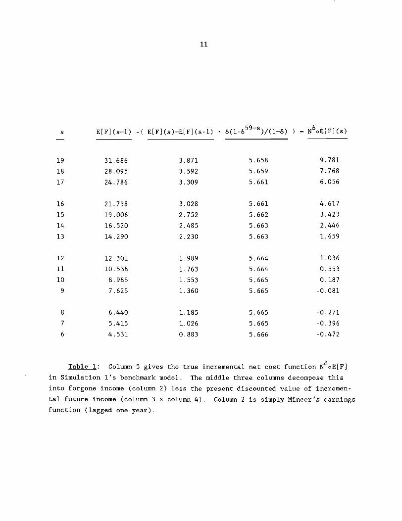
6 Table 1: Column 5 gives the true incremental net cost function N oE[F]

in Simulation 1's benchmark model. The middle three columns decompose this

into forgone income (column 2) less the present discounted value of incremen-

tal future income (column 3 x column 4). Column 2 is simply Mincer's earnings

function (lagged one year).

Figure 1 0

gg

- 4 8 12 16 20

Schooling 0.00 0.07 0.14

Density

Schooling

~igure-1: The large stars and solid curves depict Simulation 1 ' s simulation of the benchmark ,model.

See Figure lc in order to understand the distribution of taste 8 among

the hundred persons, and in order to understand their schooling choices.

Schooling appears on the horizontal axis (just as in Figure la), and taste 8

appears on the vertical axis. Each of the hundred stars represents one

person's taste 8 and schooling choice s = M~"OE[FI. Thus the stars are "log- 5

beta-ly" distributed with respect to the vertical 8 axis, and the variable s

on the horizontal axis is a function (namely s = M;'~OE[F]) of the variable 8

on the vertical axis.

For example, person 8 = 1.039 chooses a high-school education (s = 12).

This choice can be readily explained by Table 1's data and by Theorem 1's

marginal characterization. The incremental net cost of her senior year in

high school was 1.036 thousand dollars, which is the forgone income: 12.301

thousand dollars, less the present discounted value of incremental future

income: 1.989-5.664 = 11.265 thousand dollars. Since this net cost of 1.036

was less than her taste for school 8 = 1.039, she chose to finish high school.

But she quits after high school because the incremental net cost of her fresh-

man year in college (s = 13) would be 1.659, which far exceeds her taste 8.

Notice that the 14 net costs listed in Table 1 divide the clumps of stars in

Figure lc. It happens that no one's taste falls below the incremental net

cost for sixth grade, and thus, no one drops out right after fifth grade.

Return to Figure la in order to understand the random income which the

hundred persons receive. Consider person 8 = 1.039 as in the previous para-

graph. Since she chose a high-school education (s = 12), her income (y) is

lognormally distributed with mean E[F](12) = 14.290 (thousand dollars) and

standard deviation .5*E[F](12) = 7.145. In fact, 14 of the 100 persons chose

a high-school education, and their 14 random incomes are shown in Figure la as

the 14 quantiles at s = 12. Similarly, the 12 quantiles at s = 11 represent

the random incomes of the 12 persons who chose an eleventh-grade education.

Just as Figure lc, Figure la has 100 stars representing the 100 persons.

Then see Figure lb for the income distribution among the hundred individ-

uals. As in Figure la, income (y) is on the vertical axis. The income of

each person 8 has a density function equal to the derivative of the c.d.f.

F(M;"~E[F] ) . The curve in Figure lb is the average of these 100 density

functions. Casually speaking, this curve is obtained by projecting all of

Figure la's stars onto the vertical axis and letting them stack up when they

overlap. The curve swells at low incomes (say y I 20) because the lognormal

distribution is skewed, and because y is an average of lifetime income that

weights entry-level wages heavily (recall that y is the present discounted

value of lifetime income, expressed at an annual rate, with 6 = . 8 5 ) .

Finally, see Figure la to understand how a youth uses role models to

learn about the random earnings function F. The hundred stars are a represen-

tative "sample" of role models from the labor force (though quantiles are

obviously not an actual sample). For example, a youth could take the mean of

the 14 stars at s = 12 in order to estimate E[F](12), which is the expected

income of a high-school graduate. My model assumes asymptotic sampling, so

that a youth learns the entire c.d.f. F(12) rather than just a 14-observation

sample. In the extreme, I assume that she learns F(5) even though less than

one percent of the labor force has a fifth-grade education (i.e., there are no

stars at s = 5).

2.3. A Discussion of the Model's Assumptions

This section discusses the many implicit and explicit assumptions that my

model employs in order to derive sharp statements about the effect of social

isolation on schooling choice.

Schooling: My model measures schooling as years of attendance. This

measure ignores school quality, student performance, and subject area. These

three omissions clearly affect postschool income. Moreover, a student cannot

simply choose her performance. Rather she chooses school effort and this

leads to academic credentials and ultimately job opportunities in a stochastic

fashion. This could be studied by reinterpreting the model's schooling

variable as effort. The new model would then describe how role models provide

information about the relationship between effort and income, and how under-

class youth can be dissuaded from college by observing college dropouts. Yet

both young people and empirical researchers have great difficulty observing

the past effort of current workers.

Income: The model unambiguously measures income and utility (and later,

loss) in thousands of dollars because a rather specialized partial equilibrium

framework is implicitly assumed: schooling is inelastically supplied, labor

(at each schooling) is inelastically demanded, and all other markets are

simply ignored. Also ignored are possible effects from workplace discrimina-

tion, transportation costs (Kain (1968)), and the nonmarket benefits of

education (Haveman and Wolfe (1984)). These last three deficiencies could be

largely remedied by reinterpreting the model's income variable as discrimina-

tion-affected income plus nonmarket benefits less transportation costs.

: If young people observe not only the schooling and income, but also

the age of each role model, they can learn expected income as a function of

both schooling and age (given asymptotic sampling). Then they can aggregate

across time to calculate the present discounted value of lifetime earnings at

each schooling. This is a straightforward extension of the model, and Simula-

tion 1 was calibrated in precisely this fashion (see Section 2.2).

Ability: By ability I mean a variable that is positively correlated with

income at each schooling. My model assumes that at the time of her schooling

decision, a youth has no information about her ability, either directly or

through a correlation with taste 8. Thus (given asymptotic sampling) she has

no interest in observing the abilities of role models. At the other extreme,

a youth might know her own ability and observe the ability of every role model

she encounters. This poses no conceptual difficulties (given asymptotic

sampling): she would simply ignore all role models other than those having an

ability identical (or very nearly identical) to her own (see Manski (1990)).

Although matters would become far more subtle if a youth had partial knowledge

of her own and others' abilities, I don't expect that these embellishments

would fundamentally alter my conclusions.

Small Samples: If young people observe a finite sample of role models

(in contrast to the model's assumption of asymptotic sampling) and if they are

risk averse (in contrast to the model's assumption of risk-neutrality), one

would conjecture a tendency to choose the schooling levels for which there are

more role models. This conjecture complements my work: it concerns a lop-

sided distribution of the sample across schoolings rather than a biased sample

at each schooling; and it is particularly relevant if concentrated poverty is

the result of racial segregation (Massey (1990)) rather than selective out-

migration (Wilson (1987)). Shen (1989) has made some progress in formalizing

this conjecture within a Bayesian framework.

Miscellaneous: (a) Frequently, workers gain more schooling through on-

the-job training or by returning to formal schools. My schooling variable is

the first time to quit school, and the possibility of return is incorporated

into the lifetime earnings expressed in F. (b) Although my model formally

ignores the financial obstacles considered abstractly in Loury (1981) and

Ljungqvist (1989) and concretely in Manski and Wise (1983), these omitted

factors may be partially captured by varying d and 8 among individuals and

over time. (c) Young people are assumed to adjust the current income of role

models to account for the secular rise in income which will benefit them in

the future.

3. Social Isolation

3.1. Theory

I model underclass social isolation by assuming that an underclass youth

observes, for each schooling, a distribution of incomes that is truncated from

above at a. This truncation models selective out-migration from an underclass

neighborhood: everyone with income above a leaves the ghetto while everyone

with an income at or below a remains in the ghetto and provides a role model

for underclass youth. Section 7 notes that "neighborhood" (and hence "ghetto"

= underclass neighborhood) need not be interpreted geographically.

S Formally, define the truncation operator T: k++x~' -r F by

If a = +a3, the truncation operator is merely the identity function (i.e.,

there is no truncation). If a E R,+ = (0 ,+), each Ta[F] (s) is the truncated

c.d.f. generated by an asymptotic sample of the labor force with schooling s

and income y I a.

The focus of this paper is the effect of truncation on schooling choice.

As a result of truncation, an underclass youth concludes that the relationship

between schooling and income is given by the random function Ta[F] rather than

F, and thus erroneously believes that the expected income function is EoTa[F]

rather than E[ FI . This leads her to choose schooling equal to ME ' e o ~ o ~ a [ ~ ~

rather than ME'~OE[FI. Wilson's conjecture is that truncation discourages

education. This may be formalized as the statement

(where no truncation is denoted by a = i-), together with compelling examples

in which M"~OEOT~' [F] < M ~ ' ~ O E O T ~ [ F ] . 5

Although my calibrated simulations suggest that Wilson's conjecture

stands at parameter values determined by empirical studies, the theoretical

results in the remainder of this section show that conjecture (3) does not

hold at all parameter values. In fact, Counterexample 1 will exhibit a

mathematically reasonable set of parameter values for which truncation unam-

biguously encourages education. The two sources of this contrary result are

systematically investigated beforehand.

Assume for the remainder of the section that the incremental net cost

6 function N oEoTa[~] defined in Section 2.1 is weakly increasing. This assump

tion is satisfied by Counterexample 1 and Simulations 1 and 2. Given this

assumption, Theorem 1 implies that conjecture (3) is equivalent to the state-

ment that for all 6 and s,

N~OEOT~[F] (s) = 59-s EoTa[F] (s-1) - 6- ( EOT~[F] (s)-EoTa[~] (s-1) ) (1-6 )/(I-6)

increases as a falls (i.e., as truncation becomes more severe). In other

words, truncation discourages education if and only if it increases incremen-

tal net cost, where this cost was defined in Section 2.1 as forgone current

income less the present discounted value of incremental future income.

As discussed in the Introduction, the heart of Wilson's very intuitive

conjecture is that truncation (i.e., a decrease in a) flattens the regression

of income on schooling. In other words, it decreases incremental future

income and thereby increases incremental net cost. This intuition augers in

favor of conjecture (3). Unfortunately, conjecture (3) often fails for one of

two reasons.

First, truncation can very well steepen rather than flatten the regres-

sion of income on schooling. A simple and compelling example of this is

provided in Counterexample 1. The gist of this counterexample is its choice

of F, in which the densities of F(s) and F(s-1) coincide everywhere except for

a relatively small region near the lower end of their common support. When

truncation removes the upper end of their common support, it accentuates the

difference in the lower end.

Second, truncation lowers the entire regression. Specifically, trunca-

tion unambiguously reduces forgone current income, which is the first term of

incremental net cost. Therefore, incremental net cost increases only when the

decrease in incremental future income is sufficiently large to outweigh the

decrease in forgone current income. This is far from universally true in

light of the previous paragraph's demonstration that incremental future income

might even move in the wrong direction. Thus conjecture (3) is false without

parametric restrictions.

Counterexamvle 1: Define F E F by

Each F(s) describes a uniform distribution over [0,100] that has been altered

by taking the probability mass over [99,100] and adding that mass to the mass

already present at [s,s+l]. This F is extremely reasonable from a mathemati-

cal perspective. Each F(s) is continuous and its density is single-peaked.

Moreover, ( V s E ( 6 , 7 , . . . 191) F(s) first-order stochastically dominates

F(s-1).

In order to simplify the algebra, restrict your attention to truncation

cutoffs a in the interval [20,991. Notice that cr = 99 is equivalent to a = + ~ o

(i.e., no truncation) since the support of every F(s) lies within [0,99].

Given this restriction on a, the incremental net cost function may be calcu-

lated straightforwardly:

N~OEOT~[F] (s)

59-s = EoTa[F'] (5-1) - 6. ( EoTa[F] (s) - EoTa[F] (s-1) )*(I-6 ) * (1-6)-'

2 = (a +2s-1) (2a+2)-' - 6- (a+l)-'- (1-ti5'-') (1-6)-'.

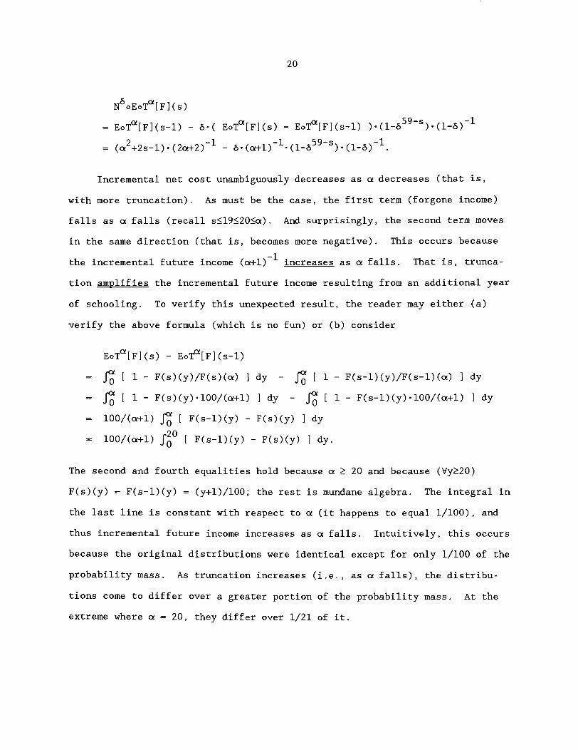
Incremental net cost unambiguously decreases as a decreases (that is,

with more truncation). As must be the case, the first term (forgone income)

falls as a falls (recall s1191201a). And surprisingly, the second term moves

in the same direction (that is, becomes more negative). This occurs because

-1 the incremental future income (a+1) increases as a falls. That is, trunca-

tion amplifies the incremental future income resulting from an additional year

of schooling. To verify this unexpected result, the reader may either (a)

verify the above formula (which is no fun) or (b) consider

EoTa[F] (s) - EoTa[F] (s-1)

= G 1 - F(s)(y)/F(s)(a) I dy - G [ 1 - F(s-l)(y)/F(s-l)(a) I dy

= G 1 - F(s)(y)*lOO/(a+l) I dy - G [ 1 - F(s-l)(y)-100/(a+l) 1 dy = 100/(a+l) G [ F(s-l)(y) - F(s)(y) I dy

= loo/(a+l) F(s-l)(y) - F(s)(y) 1 dy.

The second and fourth equalities hold because a 1 20 and because (Vy220)

F(s)(y) = F(s-l)(y) = (y+1)/100; the rest is mundane algebra. The integral in

the last line is constant with respect to a (it happens to equal 1/100), and

thus incremental future income increases as a falls. Intuitively, this occurs

because the original distributions were identical except for only 1/100 of the

probability mass. As truncation increases (i.e., as a falls), the distribu-

tions come to differ over a greater portion of the probability mass. At the

extreme where a = 20, they differ over 1/21 of it.

3.2. Simulation 2

Parameters: Simulation 2 adds social isolation to Simulation 1 by

truncating from above at the cutoff a = 16 (thousand dollars). Formally,

Simulation 2 lets s = M ~ ' ~ o E o T ~ ~ [ F ] rather than s - M~"OE[FI. Results: See Figure 2a and (for the moment) ignore the hundred stars.

As in Figure la, E[F] is depicted by the convex curve. However, since under-

class youth observe only role models below the horizontal line y = 16, they

estimate E[FI by EoT16[~], which is the curve that asymptotically approaches

the line y = 16. Note that the regression E O T ~ ~ [ F I is lower than E[F] (this

is a theoretical necessity), and that the slope of E O T ~ ~ [ F I is shallower than

that of ELF] (this results from the simulation's parameters and is not a

theoretical necessity).

See Figure 2c. For each of the hundred 8's, the large star depicts

schooling choice s = 8'80~o~16[~] under social isolation and the small star M5

depicts schooling choice s = M"~OE[F] in Simulation 1's benchmark model. As 5

Wilson predicts, social isolation depresses schooling choice. For example,

consider person 8 = 1.039, who chose s = 12 in Simulation 1's benchmark model.

Social isolation causes her to drop out after eighth grade. Ninth grade is

unattractive because she perceives its incremental net cost to be 1.906 (see

Table 2), and this exceeds her taste 8 = 1.039.

By Theorem 1's marginal characterization, Table 2's incremental net cost

function determines the steps in Simulation 2's schooling choice function.

Hence the increase of Table 2's incremental net cost function relative to

Table 1's is directly related to the decline of Simulation 2's schooling

choice relative to Simulation 1's. It is not theoretically necessary that

truncation increases incremental net costs. Rather, it is a specific feature

of the simulations' parameters (see Tables 1 and 2) that (1) truncation

decreases perceived incremental future income (e.g., from 1.360 to 0.932

59-s s EOT'~ [FI (s-1) - (EOT~~[F] (S)-EOT'~[FI (s-1)-6(1-6 )/(I-6) I = N ~ O E O T ~ ~ [ F ] (s) -

Table 2: Column 5 gives the perceived incremental net cost function

N ~ O E O T ~ ~ [ F ] in Section 2's model of social isolation. The middle three

columns decompose this into perceived forgone income (column 2) less the

perceived present discounted value of future income (column 3 x column 4).

Column 2 is the perceived earnings function (lagged one year).

0.00 0.07 0.14 Density

4 8 12 16 20 - 5 5 15 25 Schooling LOSS

Figure 2: The large stars and solid c w e s depict Simulation 2's model of social isolation. The small stars a d dotted curves recall Simulation 1's benchmark model.

thousand dollars in the case of ninth grade), and that (2) the present dis-

counted value of this decrease (e.g., 5.665*(1.360-0.932) = 2.425) is greater

than the decline in perceived forgone income (e.g., 7.625-7.184 = 0.441).

See Figure 2d for the losses borne by misinformed persons. As in Figure

2c, taste (8) is on the vertical axis. Each star gives the loss of person 8,

in thousands of dollars, as measured by

This may be interpreted as the amount of money that person 8 would be willing

to pay in order to be fully informed about E[F]. The factor 6-l2 scales this

amount to the dollars of a college freshman as opposed to those of a first

grader. For example, person 8 = 1.039 loses about 4 thousand dollars. At the

extremes, person 8 = 5.809 loses about 15 thousand dollars, and person 8 =

11.801 loses nothing because she happens to choose education efficiently even

though she is poorly informed.

Return to Figure 2a. The hundred stars depict the chosen education and

realized income of the hundred persons. Since only one person (8 = 11.801)

chose to complete three years of postgraduate education (s = 19), there is

only one quantile (at about y = 32 thousand dollars) depicting the c.d.f.

F(19). Nonetheless, asymptotic sampling enables the model's agents to esti-

mate E[F] (19) by E O T ~ ~ [ F ] (19), which is about 13 thousand dollars.

Finally, Figure 2b shows that social isolation has made Simulation 2's

income distribution lower than that of Simulation 1's benchmark.

4. Changing Role Models

4.1. Theory

This section modifies the model of the previous section by letting the

truncation cutoff a vary as an underclass youth moves through school. Her

choice of education then becomes a sequential problem: She continues on in

school if and only if the role models that she has observed up until that time

suggest that some amount of further schooling is better than stopping immedi-

ately.

Informally, we might assume that a increases over time. This would model

the notion that, as an underclass youth moves from grade school to high school

to college and finally to graduate school, the social isolation of her under-

class origins is gradually lifted. However, social isolation might well

depress her schooling choice so much so that she drops out before observing

these new role models.

S Formally, let ( ~ ( t ) ) ~ ~ ~ E R be a sequence of cutoffs. Then for t E + S

(6,7, . .19 I , define the maximization operator Mt : ( 0 , l)xRxR+ + (t , t+1, . . .19 I by

The maximization operators M6,M7,.. .M19 defined here are virtually identical

to the maximization operator M defined in Section 2. The only difference is 5

that Mt imposes the constraint s 2 t. This additional constraint is needed

momentarily so that (for example) a college freshman can't observe a fresh set

of role models and opt for a sixth-grade education. Finally, a student

chooses to quit at time t if and only if

Thus the chosen level of education is

min ( t I M;'~OEOT~(~)[F] = t I .

(I assume the change in role models is completely unanticipated, and thus

ignore the incentive to continue in school for the sake of gathering informa-

tion (Manski and Wise (1983), p. lo).)

4.2. Simulation 3

Parameters: Simulation 3 alters Simulation 2 by assuming that an under-

class youth's social isolation ends abruptly when she enters college and

consequently observes a fresh set of role models. Formally, define (a(t))tES

by setting a(t) = 16 if t I 12 and a(t) = +co if t > 12; and let schooling

choice be s = min ( t I M"~OEOT~(~)[F] = t 1, t

Results: Note that

Thus Simulation 3 is essentially an amalgamation of Simulations 1 and 2:

Social isolation causes an underclass youth to choose too little schooling (as

in Simulation 2) unless she chooses to begin college in spite of social

isolation, in which case she chooses an efficient level of schooling (as in

Simulation 1) on the basis of role models observed after entering college.

This discontinuous change in information is reflected by the stark gap in the

middle of Figure 3a, by the jumps at 8 = 7.088 in Figures 3c and 3d, and less

visibly, by the slightly fatter tail in Figure 3b relative to Figure 2b.

This discontinuity divides underclass youth into two starkly different

classes: school-loving underclass youth (8 > 7.088) who are ultimately unaf-

fected by the social isolation of their ghetto origins, and their comparative-

ly school-averse peers (8 < 7.088) who are severely harmed. This tendency to

polarization is a strong implication of my model, and it accords well with the

empirical fact that the income distribution of black men is becoming increas-

ingly polarized (Murray (1984), p. 92, citing Kilson (1981); and Wilson

(1987), p. 45, citing Levy (1986)).

Fiqure 30

4 8 12 16 2 0 Schooling

0.00 0.07 0.14 Density

a Figure 3d d I I

X

h

0 V

0 - m 0 t-

d -

u -a. K

0 a - I t

4 8 12 16 20 - 5 5 15 2 5 Schooling LOSS

Figure 3: The large stars and solid curves depict Simulation 3 ' s model of social isolation with changing role models. The small stars and dotted curves recall Simulation 1's benchmark model.

2 8

5. Welfare Effects

5.1. Theory

This section modifies the model of the previous section by assuming that

an underclass youth observes, at each schooling, a distribution of income

which is censored from below at the cutoff P. Censoring is very different

from truncating. While truncation from below at P would result in a loss of

all the probability mass below P , censoring from below at P means that all the

probability mass below P is piled up at P. This censoring models a stylized

welfare system in which everyone who has left school is guaranteed an income

of at least p. It implies that an underclass youth will observe no role

models with an income below P , and will observe an appreciable number of role

models earning exactly p.

Formally, define the censoring operator C: R X F ~ + F~ by +

If p = 0, the censoring operator is merely the identity function (i.e., there

P is no censoring). If p > 0, each C [G](s) is the cumulative distribution

function generated by censoring G(s) from below at P.

This is the final component of my model, which may be stated in its

entirety as follows. An underclass youth who is finishing grade t concludes

P that the relationship between schooling and income is C 0 ~ ~ ' ~ ) [F] , and thus

P believes that the expected income function is EoC OP(~)[F]. Because she

continues in school as long as her beliefs suggest that some amount of future

schooling is desirable, her schooling choice is

min { t 1 M~oEoc~oT~(~)[F] = t 1 .

Changing role models may be eliminated from the model by setting every at

equal to some constant parameter a, in which case schooling choice is simply

M ~ O E O C ~ O T ~ [ F ] . Truncation can then be eliminated from the model by setting

5 B a = w, in which case schooling choice is simply M oEoC [F]. This last

specialization of the model considers welfare effects only.

Unfortunately, censoring tends to violate Theorem 1's assumption by

making the expected income function very convex at low schoolings. As a

result, we cannot generally employ Theorem 1's marginal characterization of

schooling choice after censoring has taken place.

Fortunately, Theorem 2 shows that censoring has an unambiguous effect on

schooling choice. [In contrast, truncation had an ambiguous effect.] The

gist of Theorem 2's proof is that censoring unambiguously diminishes incremen-

tal future income [truncation had an ambiguous effect], and that censoring

increases forgone income [truncation decreased it]. Theorem 2 may be applied

either when G equals the true random function F (as in a model of welfare

effects alone) or when G equals T~[FI (as in a model that also includes social

isolation). Theorem 2's assumption of first-order stochastic dominance is

quite reasonable when applied to F. But it is not always satisfied when

applied to T~[F] because truncation doesn't necessarily preserve first -order

stochastic dominance.

Theorem 2: Suppose that (V s E ( 6 , 7 , . . . 19)) G(s) first-order stochas-

tically dominates G(s-1). Then (V6,8,P,P1)

A Proof: Begin by noting that if P' > p and if G(s ) first-order stochas-

B tically dominates G(s ) , then

The inequality follows from stochastic dominance and the rest is algebra.

A This observation is equivalent to the statement that if P' > fi and if G(s )

B first-order stochastically dominates G(s ) , then

E~c~'[G](s~) - E~c~'[G](s~)

B A P B I EoC [G](s ) - EoC [G](s ) .

Intuitively, this says that increased censoring (i.e., P' rather than B)

unambiguously diminishes incremental future income.

B Now fix any 6, any 8, any B' > B , and define s* = M ~ ' ~ O E O C [GI. Note

that

(Vs>s*)

U"~OEOC~' [GI (s) - U~'~OEOC" [GI (s*)

= cS a=s*+l 9-EOC" [GI (s*) I + x5' EoCB' [GI (s)-EoCB ' [GI (s*) )

a=s+l s &a-1

-< ea=s*+l ( 8-EoCBIG] (s*) 1 + c5' a=s+l EoCB'[G] (s)-EoCB'[G] (s*) )

&a-1 e:=s*+l ( 8-Eo2 [GI (s*) I + x5' a=s+l ba-l B ( EoC [G](s)-EoCBIG](s*) I

= U"~OEOC~ [GI (s) - U~"OEOC~ [GI (s*)

B The first inequality follows from the fact that EOC" [GI (s*) 2 EoC [GI (s*)

(that is, censoring increases forgone income); the second inequality follows

from the preceding paragraph (that is, censoring diminishes incremental future

income since F(s) first-order stochastically dominates F(s*)); the final

inequality follows from the definition of s*; and the equalities are just

algebra. Since the first line is the objective function evaluated at s less

the objective function evaluated at s*, the entire result implies that

which by the definition of s* is equivalent to

Although an underclass youth is prudent to consider post- rather than

pre-transfer income when making her individual decisions, welfare leads her to

make decisions that are quite inefficient from the perspective of society as a

whole. To be precise, let s* = M"~OE[F] be choice in the benchmark model 5

with no distortions and let s' = min { t 1 M~'~OEOC~OT~(~)[F] = t ) be choice

with social isolation and welfare. Since the objective function is defined in

a way that makes income and utility directly comparable, and under the assump-

tion that the social and individual discount factor coincide, we may unambigu-

ously calculate the loss to society as

U"~OE[F] (s*) - U"~OE[F] (st) (4)

= [ u"~oE[F](s*) - u"~oEoc~[F](s') ] + [ U~'~OEOC~[FI(S') - u"~~E[FI(~') 1 P 59 EocPIF] (st )-E[F] (sf) 1. - [ u"~oE[F](s*) - U"~OEOC [F](sl) 1 + Ea=st+l

The first term is the loss to the individual, which can be negative given a

sufficiently generous welfare program. The second term is the expected

present discounted value of the government's welfare expenditures, which

cannot be negative. Since the sum of the two terms cannot be negative (be-

cause s* is defined to be a maximizer of u6"oE [ F] ) , the individual gains (if

any) are overwhelmed by the government's expenditures.

The effect of social isolation on underclass schooling is not diminished

by the effect of welfare. Rather, Simulations 4 and 5 demonstrate that the

two mechanisms tend to depress schooling choice through distinct and reinforc-

ing channels. In fact, I am tempted to conclude that the effects of social

isolation and welfare are not only additive, but even superadditive. Essen-

tially, social isolation destroys incentives through the loss of high-income

role models while welfare destroys incentives by altering the experience of

low-income role models. Distortions on one side make the distortions on the

other side even more critical.

5.2. Simulation 4

Parameters: Simulation 4 specifies F, 6, and 9 as in Section 1's bench-

mark model; it assumes no social isolation (i.e., a = -); and it studies the

effects of a welfare program which censors income at the level P = 4. Formal-

4 ly, let s = M~"OEOC [F]. 5

Results: Theorem 2 tells us that welfare monotonically depresses school-

ing choice. Simulation 4 reveals that this effect can be quite severe: 26

percent of the simulation's hundred persons drop out after fifth grade, which

is the model's lower bound on schooling choice (Figures 4a, 4c). This con-

trasts markedly with the benchmark model in which no one drops out this early

(Figures la, lc). Moreover, the cutoff level P = 4 is rather moderate. It

lies everywhere below the true expected income function E[F].

While social isolation shifts all but the upper tail of the distribution

of schooling choice (Simulation 3), welfare's main effect is to entrap the

lower tail at s = 5. The most severely affected person is 9 = 0.677, who

dropped out after fifth grade even though she should have chosen an eleventh-

grade education. Her decision creates a loss of 11 thousand dollars (Figure

4d), as measured by equation (4). (Some other schooling choices that are not

in the lower tail are also affected. For example, person 9 = 1.036 chooses

s = 11 rather than s = 12 (Figure 4c), but her utility loss is insignificant

(Figure 4d).)

Figure 40

0 0 4 8 12 16 2 0 0.00 0.07 0.14

Schooling Density

- 5 5 15 25 Loss

.. - --

~l Figure 4d

uaure 4 : The large stars and so l id curves depict Simulation 4 ' s model of welfare effects . The small stars and dotted curves recall Simulation 1's benchmark model.

d

h

n e9

0 . w

U &

Y ) ' 0 + d

0 -

-cn

0 I

I I

X

-

-

-

X

-

-

-

; / 3

K I I

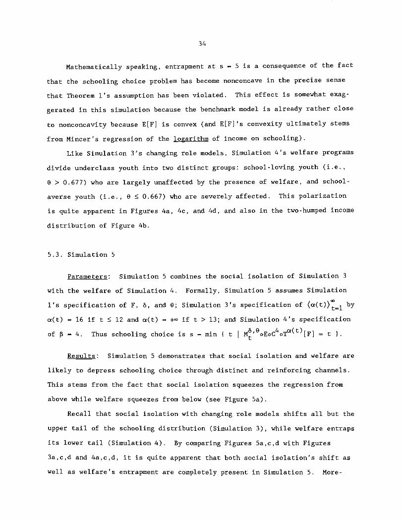
Mathematically speaking, entrapment at s = 5 is a consequence of the fact

that the schooling choice problem has become nonconcave in the precise sense

that Theorem 1's assumption has been violated. This effect is somewhat exag-

gerated in this simulation because the benchmark model is already rather close

to nonconcavity because E[F] is convex (and E[F]'s convexity ultimately stems

from Mincer's regression of the logarithm of income on schooling).

Like Simulation 3's changing role models, Simulation 4's welfare programs

divide underclass youth into two distinct groups: school-loving youth (i.e.,

8 > 0.677) who are largely unaffected by the presence of welfare, and school-

averse youth (i.e., 8 I 0.667) who are severely affected. This polarization

is quite apparent in Figures 4a, 4c, and 4d, and also in the two-humped income

distribution of Figure 4b.

5.3. Simulation 5

Parameters: Simulation 5 combines the social isolation of Simulation 3

with the welfare of Simulation 4. Formally, Simulation 5 assumes Simulation Ln

1's specification of F, 6, and 8; Simulation 3's specification of (a(t)) t=l by

a(t) = 16 if t I 12 and a(t) = ~ Q J if t > 13; and Simulation 4's specification

of = 4. Thus schooling choice is s = min ( t I M'"OEOC~OT~( t, [F] = t ) . t

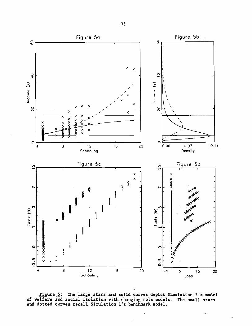
Results: Simulation 5 demonstrates that social isolation and welfare are

likely to depress schooling choice through distinct and reinforcing channels.

This stems from the fact that social isolation squeezes the regression from

above while welfare squeezes from below (see Figure 5a).

Recall that social isolation with changing role models shifts all but the

upper tail of the schooling distribution (Simulation 3), while welfare entraps

its lower tail (Simulation 4). By comparing Figures 5a,c,d with Figures

3a,c,d and 4a,c,d, it is quite apparent that both social isolation's shift as

well as welfare's entrapment are completely present in Simulation 5. More-

4 8 12 16 20 Schooling

0.00 0.07 0.14 Density

Figure 5d =-

4 8 12 16 20 - 5 5 15 2 5 Schooling LOSS

Fieure 9: The large stars and solid curves depict Simulation 5 ' s model of welfare and social isolation with changing role models. The small stars and dotted curves recall Simulation 1's benchmark model.

over, there is a reinforcing interaction: social isolation's shift enables

welfare to entrap a larger tail. In particular, 45 percent of the hundred

persons are entrapped by welfare in the social isolation of the ghetto (Simu-

lation 5), even though only 26 percent would have been entrapped outside the

ghetto (Simulation 4). The greatest loss is created by someone in this extra

19 percent: Person 8 = 1.487 should have chosen a high-school education, but

instead dropped out after fifth grade and thereby created a loss of about 22

thousand dollars (Figure 5d), as measured by equation (4).

6. Further Simulations

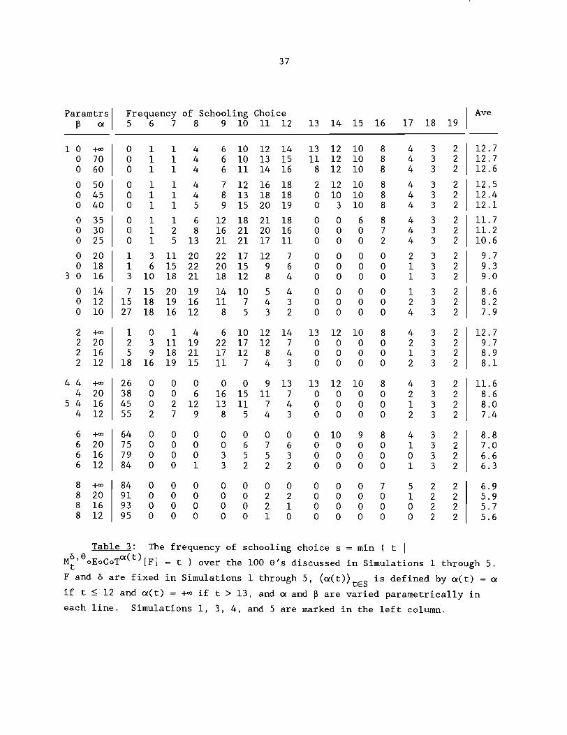
Table 3 offers a number of simulations which tweak the parameters of

Simulations 1, 3, 4, and 5. These additional simulations will help you gauge

the validity of the conclusions I have drawn. Note how bad things get as the

cutoffs a and p converge.

7. Empirical Comments

This section builds a bridge to related empirical work in order to

demonstrate the empirical relevance of my theory and in order to suggest new

avenues of empirical research.

By neighborhood, I mean the collection of role models from the labor

force which a youth observes. Such a neighborhood is geographic (as in

Hughes' (1989) careful definition) to the extent that residential proximity

and social interaction are highly correlated. This correlation increases as

stores, schools, and social institutions draw from smaller geographic areas.

More generally, my neighborhoods could be regarded as nongeographic entities

such as schools (as below), friendship networks, religious institutions, or

groups maintaining an ethnic identity. As in a geographic neighborhood,

social isolation occurs within a nongeographic neighborhood when there is

Paramtrs Frequency of Schooling Choice p a 5 6 7 8 9 10 11 12 13 14 15 16 17 18 19 1 Ave

Table 3: The frequency of schooling choice s = min ( t I M~'~oEocoT~(~)[F] = t I over the 100 0's discussed in Simulations 1 through 5. F and d are fixed in Simulations 1 through 5, ( ~ ( t ) ) ~ ~ ~ is defined by a(t) = a

if t I 12 and a(t) = +co if t > 13, and a and p are varied parametrically in each line. Simulations 1, 3, 4, and 5 are marked in the left column.

selective out-migration by high-income role models (or equivalently, selective

in-migration by low-income role models).

The theory predicts that socially isolated neighborhoods (i.e., ghettos)

engender inefficient schooling choices. This prediction is only tenuously

related to the statement that mean neighborhood income depresses schooling

choice. First, there is the theoretical possibility that social isolation

increases schooling choice (Counterexample 1). This concern is somewhat

ameliorated by calibrated simulations which confirm the expected effect

(Simulation 2).

Second, and more importantly, the theory clarifies that schooling choice

is inefficient when a youth's perception of the earnings function is distorted

by an unrepresentative neighborhood, and the representativeness of a neighbor-

hood need not have anything to do with its mean income. For example, suppose

that there are three neighborhoods: a lower-class neighborhood truncated from

above at an income of 16 thousand dollars (as in Simulation 2); a middle-class

neighborhood that is perfectly representative of the labor market; and an

upper-class neighborhood truncated from below at an income of 40 thousand

dollars (this can be simulated by the GAUSS procedure ECTL). In this example,

the graph of schooling choice as a function of mean neighborhood income would

be an upside-down U. Thus a linear regression of schooling choice on neigh-

borhood income could very well be flat or even downward sloping (when one

controls for parental income). This observation accords very well with Jencks

and Mayer's ((1990), pages 123-125, and 177) suggestion that empirical re-

searchers be concerned with nonlinear relationships.

Given these weighty caveats, I turn to linear regressions of schooling

choice on mean neighborhood income and socioeconomic status, and draw heavily

from Jencks and Mayer's (1990) excellent survey. Datcher (1982) and Corcoran

et al. (1987) study geographic neighborhoods and provide evidence in support

of the theory. For example, Datcher finds that a $1000 increase in mean

neighborhood income (measured in 1970 dollars) increases schooling by about

one-tenth of a year (the estimate is .087 (with a standard error of .061) for

blacks, and .I03 (.035) for whites). This is roughly the magnitude predicted

by the means in Table 3, if one takes a to be about twice mean neighborhood

income.

On the other hand, many researchers, including Meyer (1970) and Jencks et

al. (1972), have regressed a youth's schooling choice on the mean socioeconom-

ic status of families with children in her school. The consensus of these

studies supports the theory by finding that schooling is positively correlated

with mean school socioeconomic status when one controls for mean school test

scores (Jencks and Mayer (1990), pages 127-130 and Jencks et al. (1972), pages

151-153).

Perhaps future empirical work will regress schooling choice on a better

measure of social isolation, and simulate the model with more finely calibrat-

ed parameters.

REFERENCES

Corcoran, Mary, Roger Gordon, Deborah Laren, and Gary Solon (1987): "Intergen- erational Transmission of Education, Income, and Earnings," University of Michigan, Political Science Department, mimeo.

Datcher, Linda (1982): "Effects of Community and Family Background on Achieve- ment," Review of Economics and Statistics 64, 32-41.

Haveman, Robert and Barbara Wolfe (1984): "Schooling and Economic Well-Being: The Role of Nonmarket Effects," Journal of Human Resources 19, 377-407.

Heckman, James J. (1976): "A Life-Cycle Model of Earnings, Learning, and Consumption," Journal of Political Economy 84, Number 4, Part 2, Sll-S44.

Hughes, Mark Alan (1989): "Misspeaking Truth to Power: A Geographical Perspec- tive on the 'Underclass' Fallacy," Economic Geography 65, 187-207.

Jencks, Christopher et al. (1972): Inequality: A Reassessment of the Effect of Family and Schooling - in America, Harper and Row, New York.

Jencks, Christopher and Susan E. Mayer (1990): "The Social Consequences of Growing Up in a Poor Neighborhood," in Laurence E. Lynn, Jr., and Michael G.H. McGeary (eds.), Inner-City Poverty in the United States, National Academy Press, Washington, DC.

Kain, John F. (1968): "Housing Segregation, Negro Employment, and Metropolitan Decentralization," Quarterly Journal of Economics 82, 175-197.

Kilson, Martin (1981): "Black Social Classes and Intergenerational Poverty," Public Interest, Summer, 58-78.

Levy, F. (1986): "Poverty and Economic Growth," University of Maryland, mimeo.

Ljungqvist, Lars (1989): "Insufficient Human Capital Accumulation Resulting in a Dual Economy Caught in a Poverty Trap," University of Wisconsin-Madi- son, Institute for Research on Poverty, Discussion Paper 875-89.

Loury, Glenn C. (1981): "Intergenerational Transfers and the Distribution of Earnings," Econometrica 49, 843-867.

Manski, Charles (1990): "Dynamic Choice in a Social Setting," University of Wisconsin-Madison, Department of Economics, mimeo.

Manski, Charles F. and David A. Wise (1983): College Choice in America, Har- vard University Press, Cambridge, MA.

Massey, Douglas S. (1990): "American Apartheid: Segregation and the Making of the Underclass," American Journal of Sociology 96, 329-357.

Meyer, John W. (1970): "High School Effects on College Intentions," American Journal of Sociology 76, 59-70.

Mincer, Jacob (1974): Schooling, Experience and Earnin~s, National Bureau of Economic Research, Columbia University Press, New York.

Mood, Alexander M., Franklin A. Graybill, and Duane C. Boes (1974): Introduc- tion to the Theory of Statistics, McGraw-Hill, New York.

Murray, Charles (1984): Losing Ground: American Social Policy, 1950-1980, Basic Books, New York.

Rosen, Sherwin (1977): "Human Capital: A Survey of Empirical Research," in Ronald G. Ehrenberg (ed.), Research in Labor Economics, Vol. 1, JAI Press, Greenwich, CT.

Ryder, Harl E., Frank P. Stafford and Paula E. Stephan (1976): "Labor, Leisure and Training over the Life Cycle," International Economic Review 17, 651- 674.

Shen, Theodore (1989): "A Model of Occupational Aspirations under Incomplete Information," University of Wisconsin-Madison, Economics Department, mimeo .

U.S. Bureau of the Census (1990): Statistical Abstract of the United States, 1990, U.S. Government Printing Office, Washington, DC.

U.S. Council of Economic Advisers (1991): Economic Indicators. March 1991, U.S. Government Printing Office, Washington, DC.

Willis, Robert J. (1986): "Wage Determinants: A Survey and Reinterpretation of Human Capital Earnings Functions," in Orley C. Ashenfelter and Richard Layard (eds.), Handbook of Labor Economics. Volume 1, North-Holland, Amsterdam.

Wilson, William Julius (1987): The Truly Disadvantaged: The Inner City, the Underclass, and Public Policy, University of Chicago Press, Chicago.