
2D Fluid Turbulence (Merz)
36
ASDEX Upgrade Max−Planck−Institut für Plasmaphysik 2D Fluid Turbulence Florian Merz Seminar on Turbulence, 08.09.05
Transcript of 2D Fluid Turbulence (Merz)
8/3/2019 2D Fluid Turbulence (Merz)
http://slidepdf.com/reader/full/2d-fluid-turbulence-merz 1/36
ASDEX Upgrade
Max−Planck−Institutfür Plasmaphysik
2D Fluid Turbulence
Florian Merz
Seminar on Turbulence, 08.09.05
8/3/2019 2D Fluid Turbulence (Merz)
http://slidepdf.com/reader/full/2d-fluid-turbulence-merz 2/36
2D turbulence?
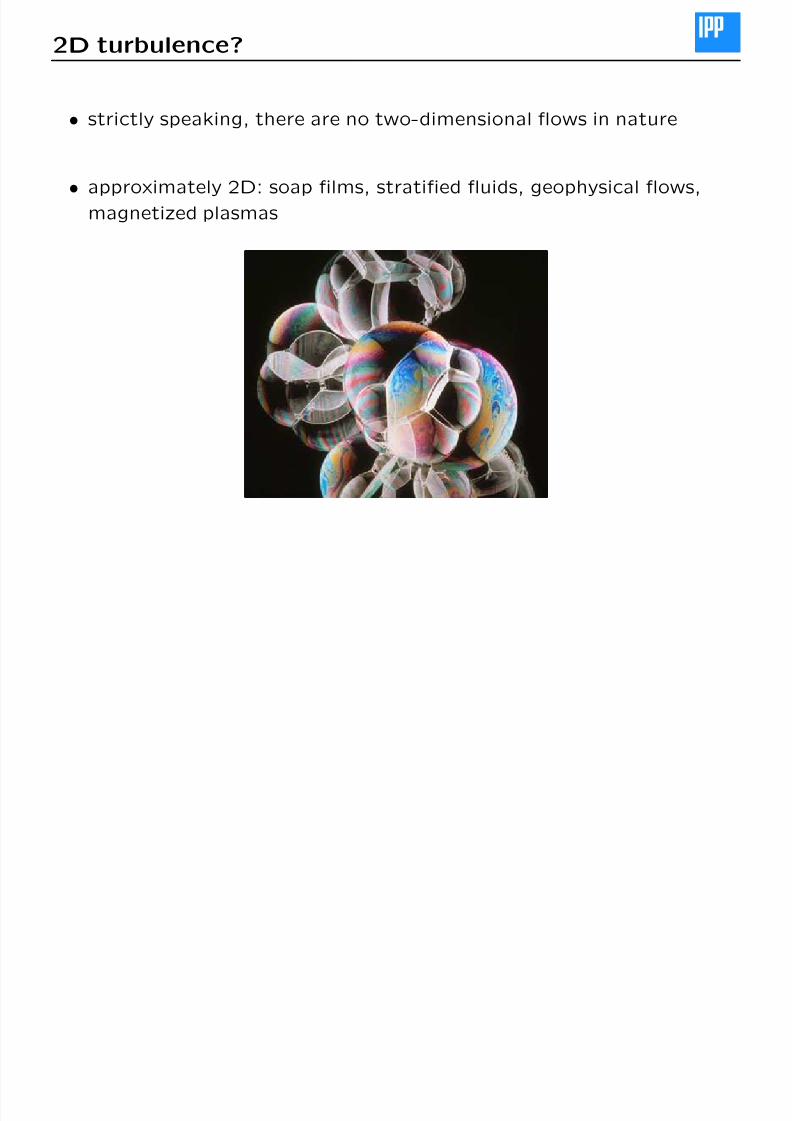
• strictly speaking, there are no two-dimensional flows in nature
• approximately 2D: soap films, stratified fluids, geophysical flows,magnetized plasmas
8/3/2019 2D Fluid Turbulence (Merz)
http://slidepdf.com/reader/full/2d-fluid-turbulence-merz 3/36
2D turbulence?
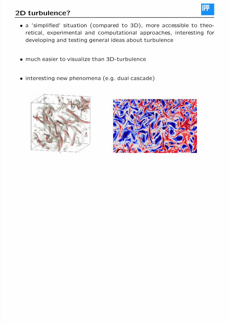
• a ’simplified’ situation (compared to 3D), more accessible to theo-retical, experimental and computational approaches, interesting for
developing and testing general ideas about turbulence
• much easier to visualize than 3D-turbulence
•interesting new phenomena (e.g. dual cascade)

8/3/2019 2D Fluid Turbulence (Merz)
http://slidepdf.com/reader/full/2d-fluid-turbulence-merz 4/36
Outline
• Basic equations
• Cascades in 2D
• Coherent structures
8/3/2019 2D Fluid Turbulence (Merz)
http://slidepdf.com/reader/full/2d-fluid-turbulence-merz 5/36
Basic equations: velocity
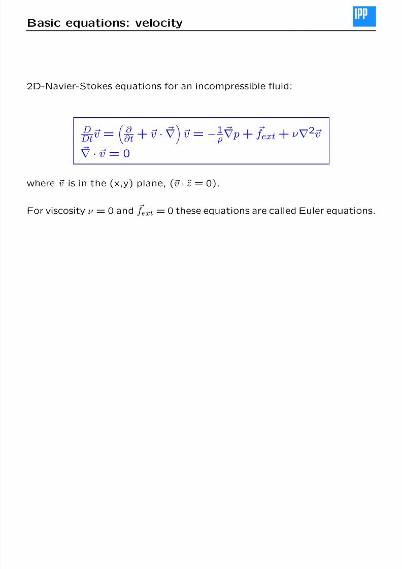
2D-Navier-Stokes equations for an incompressible fluid:
DDtv =
∂ ∂t + v · v = −
1ρ p + f ext + ν 2v
· v = 0
where v is in the (x,y) plane, (v · z = 0).
For viscosity ν = 0 and f ext = 0 these equations are called Euler equations.
8/3/2019 2D Fluid Turbulence (Merz)
http://slidepdf.com/reader/full/2d-fluid-turbulence-merz 6/36
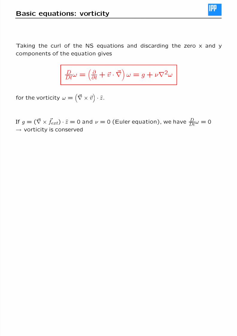
Basic equations: vorticity
Taking the curl of the NS equations and discarding the zero x and y
components of the equation gives
DDtω =
∂ ∂t + v ·
ω = g + ν 2ω
for the vorticity ω =
× v· z.
If g = ( × f ext) · z = 0 and ν = 0 (Euler equation), we have DDtω = 0
→ vorticity is conserved
8/3/2019 2D Fluid Turbulence (Merz)
http://slidepdf.com/reader/full/2d-fluid-turbulence-merz 7/36
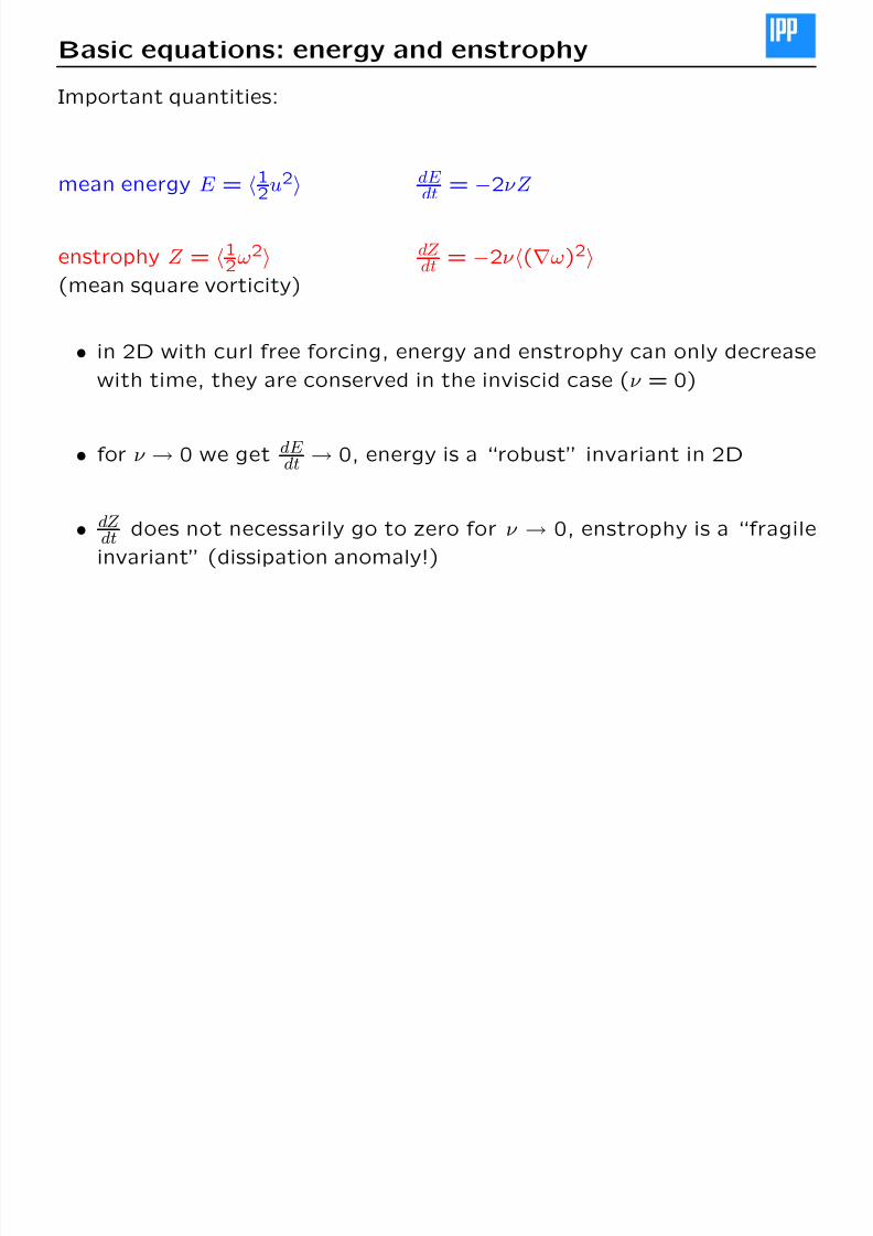
Basic equations: energy and enstrophy
Important quantities:
mean energy E = 12u2
enstrophy Z = 12ω2
(mean square vorticity)
dE dt = −2νZ
dZ dt = −2ν (ω)2
• in 2D with curl free forcing, energy and enstrophy can only decrease
with time, they are conserved in the inviscid case (ν = 0)
• for ν → 0 we get dE dt → 0, energy is a “robust” invariant in 2D
•dZ
dt does not necessarily go to zero for ν → 0, enstrophy is a “fragileinvariant” (dissipation anomaly!)
8/3/2019 2D Fluid Turbulence (Merz)
http://slidepdf.com/reader/full/2d-fluid-turbulence-merz 8/36
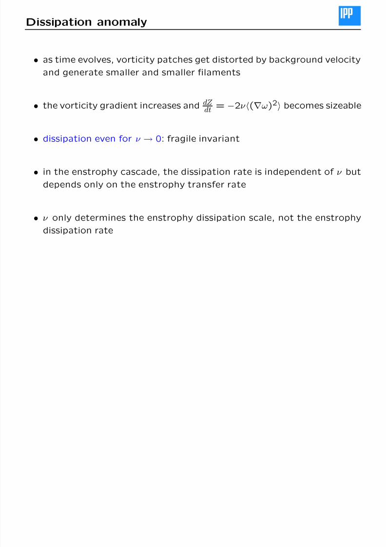
Dissipation anomaly
• as time evolves, vorticity patches get distorted by background velocity
and generate smaller and smaller filaments
• the vorticity gradient increases and dZ dt = −2ν (ω)2 becomes sizeable
• dissipation even for ν → 0: fragile invariant
• in the enstrophy cascade, the dissipation rate is independent of ν but
depends only on the enstrophy transfer rate
• ν only determines the enstrophy dissipation scale, not the enstrophy
dissipation rate
8/3/2019 2D Fluid Turbulence (Merz)
http://slidepdf.com/reader/full/2d-fluid-turbulence-merz 9/36
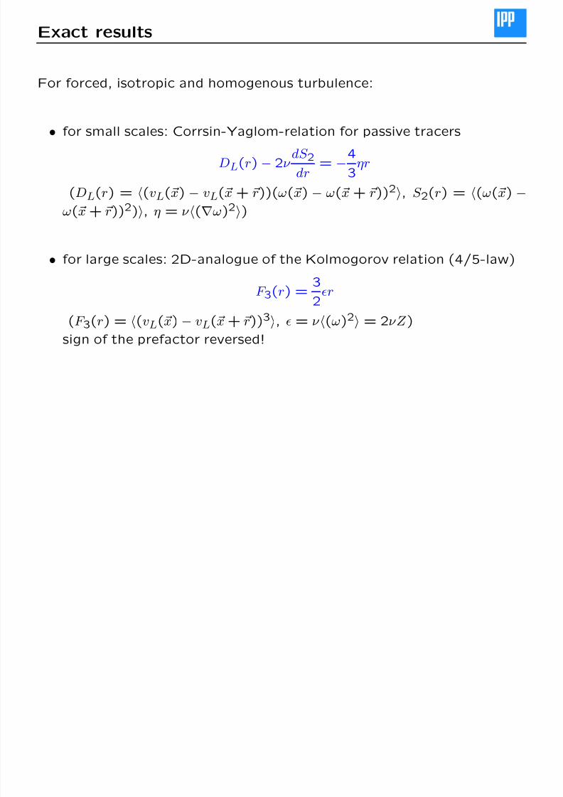
Exact results
For forced, isotropic and homogenous turbulence:
•for small scales: Corrsin-Yaglom-relation for passive tracers
DL(r)− 2ν dS 2dr
= −4
3ηr
(DL(r) =
(vL(x)
−vL(x + r))(ω(x)
−ω(x + r))2
, S 2(r) =
(ω(x)
−ω(x + r))2), η = ν (ω)2)
• for large scales: 2D-analogue of the Kolmogorov relation (4/5-law)
F 3(r) =3
2r
(F 3(r) = (vL(x)− vL(x + r))3, = ν (ω)2 = 2νZ )
sign of the prefactor reversed!

8/3/2019 2D Fluid Turbulence (Merz)
http://slidepdf.com/reader/full/2d-fluid-turbulence-merz 10/36
Cascades
8/3/2019 2D Fluid Turbulence (Merz)
http://slidepdf.com/reader/full/2d-fluid-turbulence-merz 11/36
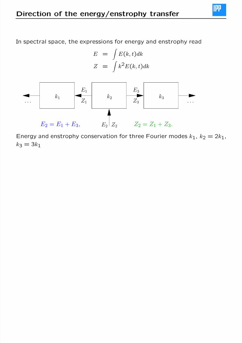
Direction of the energy/enstrophy transfer
In spectral space, the expressions for energy and enstrophy read
E = E (k, t)dk
Z =
k2E (k, t)dk
. . .k2 k3k1
Z 1 Z 3
Z 2
E 1 E 3
. . .
E 2E 2 = E 1 + E 3, Z 2 = Z 1 + Z 3.
Energy and enstrophy conservation for three Fourier modes k1, k2 = 2k1,
k3 = 3k1
8/3/2019 2D Fluid Turbulence (Merz)
http://slidepdf.com/reader/full/2d-fluid-turbulence-merz 12/36
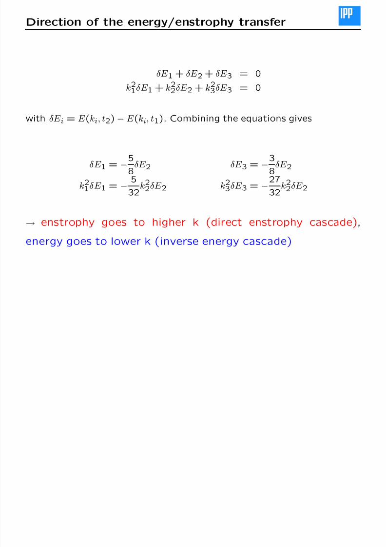
Direction of the energy/enstrophy transfer
δE 1 + δE 2 + δE 3 = 0
k21δE 1 + k2
2δE 2 + k23δE 3 = 0
with δE i = E (ki, t2)− E (ki, t1). Combining the equations gives
δE 1 = −5
8δE 2 δE 3 = −3
8δE 2
k2
1δE
1=−
5
32k2
2δE
2k2
3δE
3=−
27
32k2
2δE
2
→ enstrophy goes to higher k (direct enstrophy cascade),
energy goes to lower k (inverse energy cascade)
8/3/2019 2D Fluid Turbulence (Merz)
http://slidepdf.com/reader/full/2d-fluid-turbulence-merz 13/36
Direction of the energy/enstrophy transfer
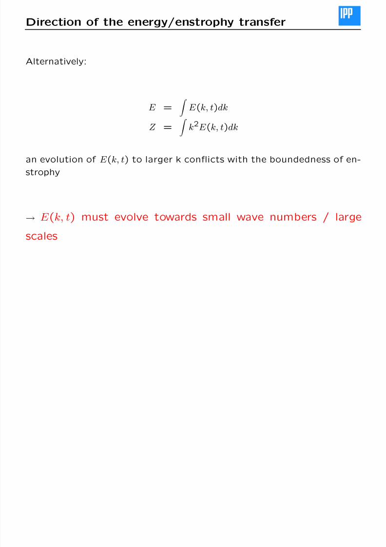
Alternatively:
E =
E (k, t)dk
Z =
k2E (k, t)dk
an evolution of E (k, t) to larger k conflicts with the boundedness of en-
strophy
→ E (k, t) must evolve towards small wave numbers / large
scales
8/3/2019 2D Fluid Turbulence (Merz)
http://slidepdf.com/reader/full/2d-fluid-turbulence-merz 14/36
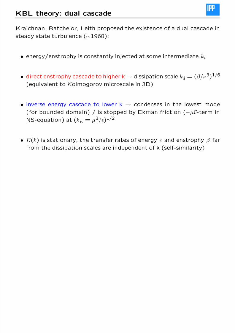
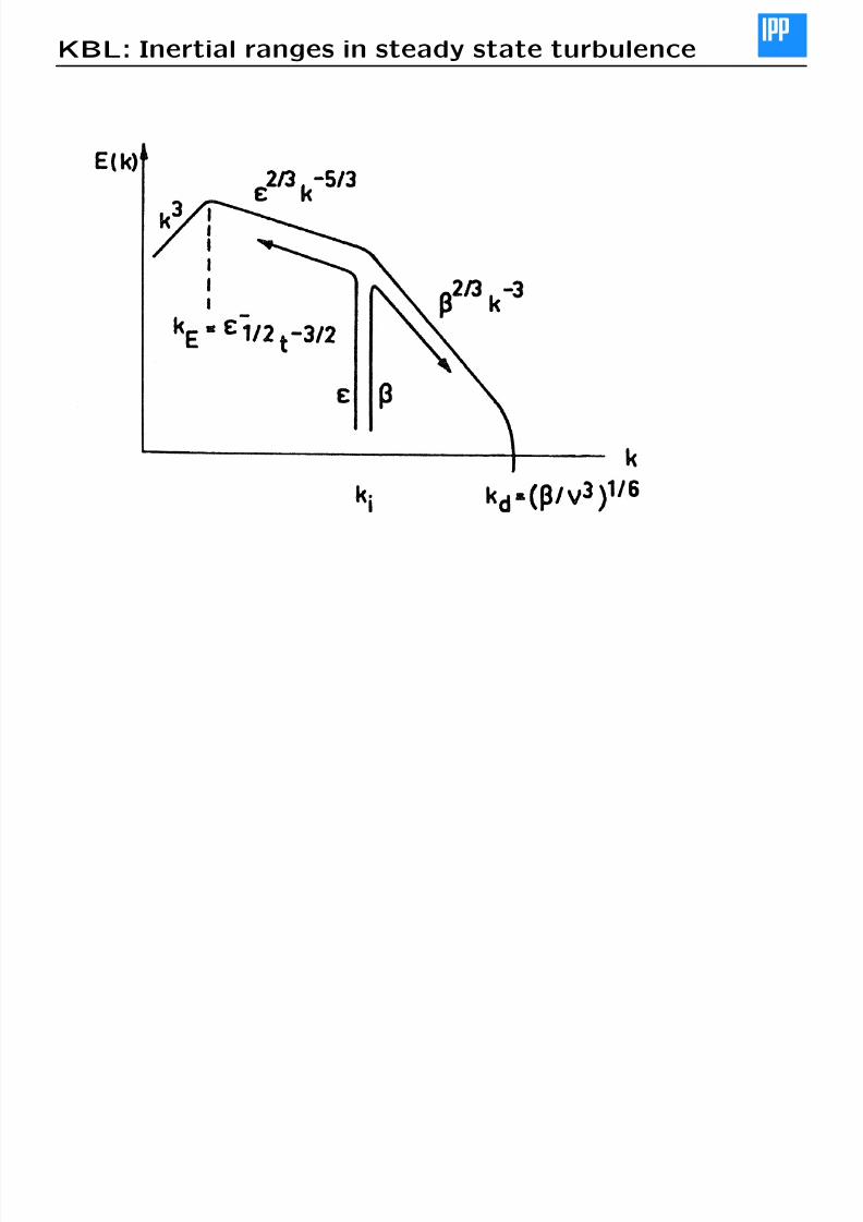
KBL theory: dual cascade
Kraichnan, Batchelor, Leith proposed the existence of a dual cascade insteady state turbulence (∼1968):
• energy/enstrophy is constantly injected at some intermediate ki
• direct enstrophy cascade to higher k → dissipation scale kd = (β/ν 3)1/6
(equivalent to Kolmogorov microscale in 3D)
• inverse energy cascade to lower k → condenses in the lowest mode
(for bounded domain) / is stopped by Ekman friction (
−µv-term in
NS-equation) at (kE = µ3/)1/2
•E (k) is stationary, the transfer rates of energy and enstrophy β far
from the dissipation scales are independent of k (self-similarity)
8/3/2019 2D Fluid Turbulence (Merz)
http://slidepdf.com/reader/full/2d-fluid-turbulence-merz 15/36
KBL theory: inertial ranges
• inertial range of the energy cascade: for kE k ki, the energy
spectrum can only depend on .
Dimensional analysis:
k = [L]−1; E (k) = [L]3[T ]−2; = [L]2[T ]−3 → E (k) = C2/3k−5/3
• inertial range of the enstrophy cascade (ki k kd): the energy
spectrum can only depend on β .Dimensional analysis:
k = [L]−1; E (k) = [L]3[T ]−2; β = [T ]−3 → E (k) = C β 2/3k−3
C, C constant and dimensionless.
• zero enstrophy transfer in the energy inertial range, zero energy trans-
fer in the enstrophy inertial range
8/3/2019 2D Fluid Turbulence (Merz)
http://slidepdf.com/reader/full/2d-fluid-turbulence-merz 16/36
KBL: Inertial ranges in steady state turbulence
8/3/2019 2D Fluid Turbulence (Merz)
http://slidepdf.com/reader/full/2d-fluid-turbulence-merz 17/36
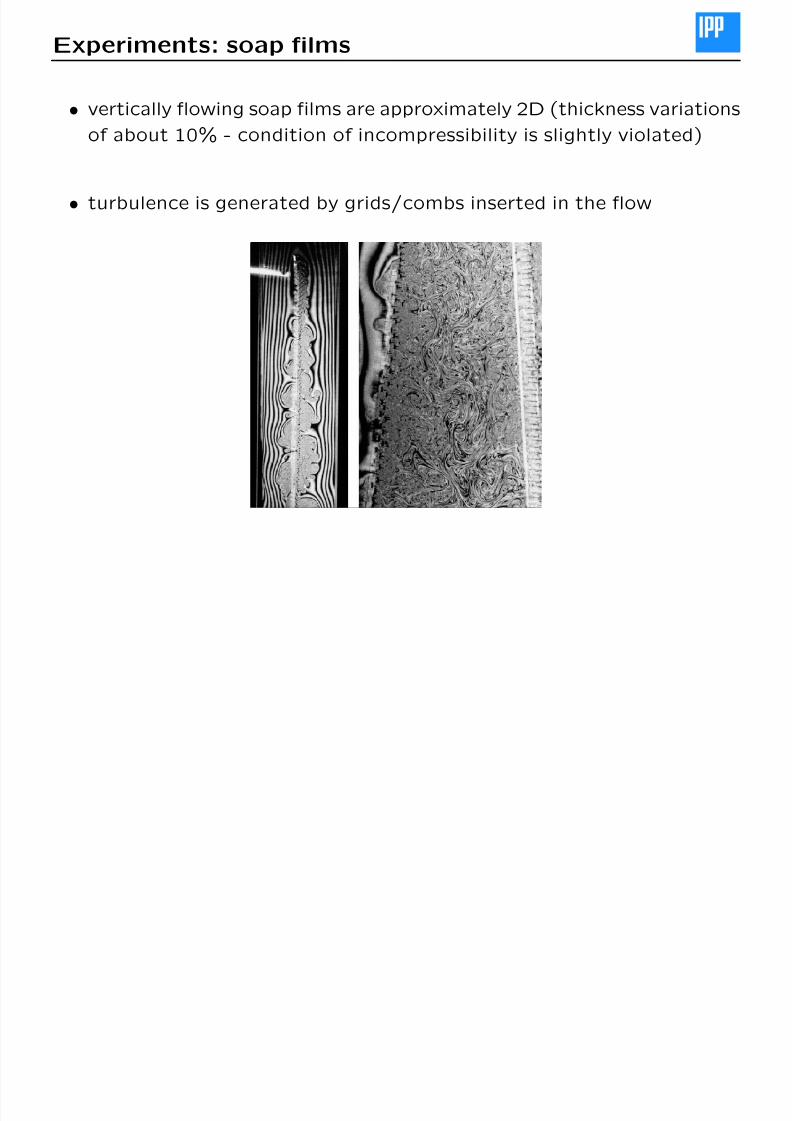
Experiments: soap films
• vertically flowing soap films are approximately 2D (thickness variations
of about 10% - condition of incompressibility is slightly violated)
• turbulence is generated by grids/combs inserted in the flow
8/3/2019 2D Fluid Turbulence (Merz)
http://slidepdf.com/reader/full/2d-fluid-turbulence-merz 18/36
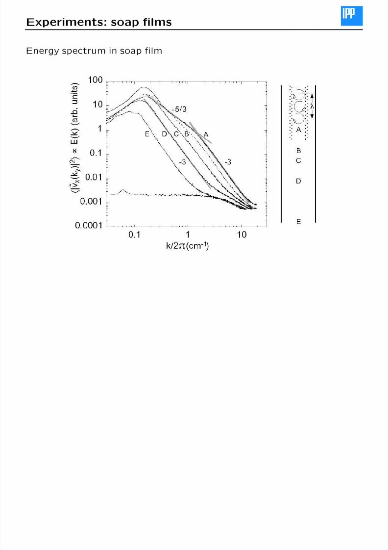
Experiments: soap films
Energy spectrum in soap film
8/3/2019 2D Fluid Turbulence (Merz)
http://slidepdf.com/reader/full/2d-fluid-turbulence-merz 19/36
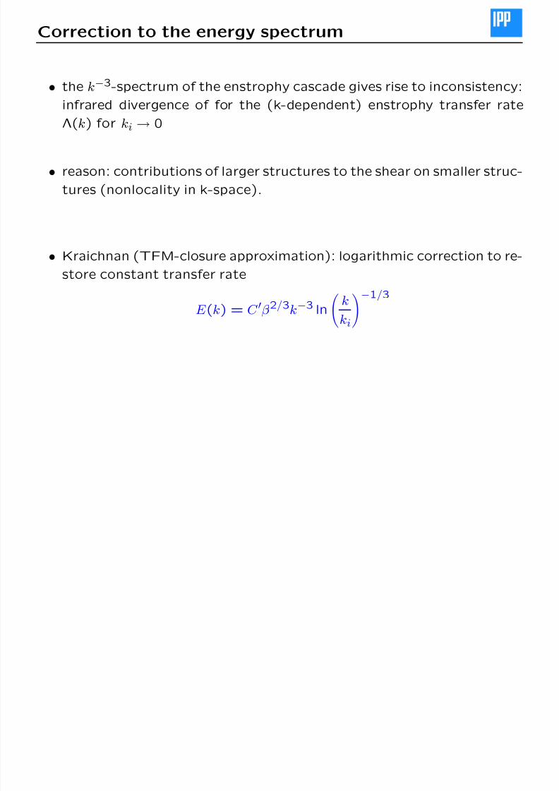
Correction to the energy spectrum
• the k−3-spectrum of the enstrophy cascade gives rise to inconsistency:
infrared divergence of for the (k-dependent) enstrophy transfer rate
Λ(k) for ki → 0
• reason: contributions of larger structures to the shear on smaller struc-
tures (nonlocality in k-space).
• Kraichnan (TFM-closure approximation): logarithmic correction to re-
store constant transfer rate
E (k) = C β 2/3k−3 ln
k
ki
−1/3
8/3/2019 2D Fluid Turbulence (Merz)
http://slidepdf.com/reader/full/2d-fluid-turbulence-merz 20/36
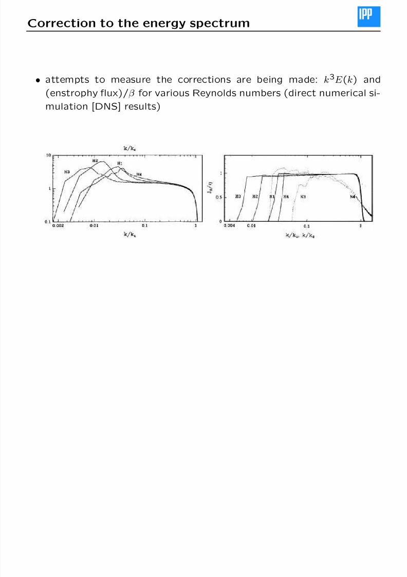
Correction to the energy spectrum
• attempts to measure the corrections are being made: k3E (k) and
(enstrophy flux)/β for various Reynolds numbers (direct numerical si-
mulation [DNS] results)
8/3/2019 2D Fluid Turbulence (Merz)
http://slidepdf.com/reader/full/2d-fluid-turbulence-merz 21/36
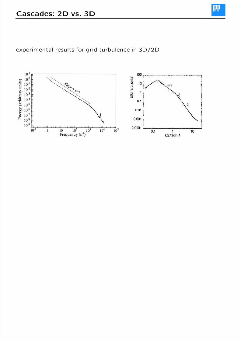
Cascades: 2D vs. 3D
Vorticity equation in 3 dimensions (analogous to MHD kinematic equation
for ω →
B
):
D
Dt ω = ( ω · )v + g + ν 2 ω
the additional vortex-stretching term changes the behaviour significantly:
• gradients in the velocity field stretch embedded vortex tubes
• as the cross section decreases, the vorticity increases
8/3/2019 2D Fluid Turbulence (Merz)
http://slidepdf.com/reader/full/2d-fluid-turbulence-merz 22/36
Cascades: 2D vs. 3D
• enstrophy in 3D is not conserved even for ν = 0 but increases with
time (in 2D: fragile invariant) → no enstrophy cascade in 3D!
• energy in 3D follows dE dt = −2νZ and is a fragile invariant (in 2D:
robust invariant)
• energy cascades to smaller scales in 3D (direct cascade), in 2D to
large scales (inverse cascade)
• E (k) has the same k−5/3-dependence in the inertial range of the ener-
gy cascade
8/3/2019 2D Fluid Turbulence (Merz)
http://slidepdf.com/reader/full/2d-fluid-turbulence-merz 23/36
Cascades: 2D vs. 3D
experimental results for grid turbulence in 3D/2D

8/3/2019 2D Fluid Turbulence (Merz)
http://slidepdf.com/reader/full/2d-fluid-turbulence-merz 24/36
Coherent structures
8/3/2019 2D Fluid Turbulence (Merz)
http://slidepdf.com/reader/full/2d-fluid-turbulence-merz 25/36
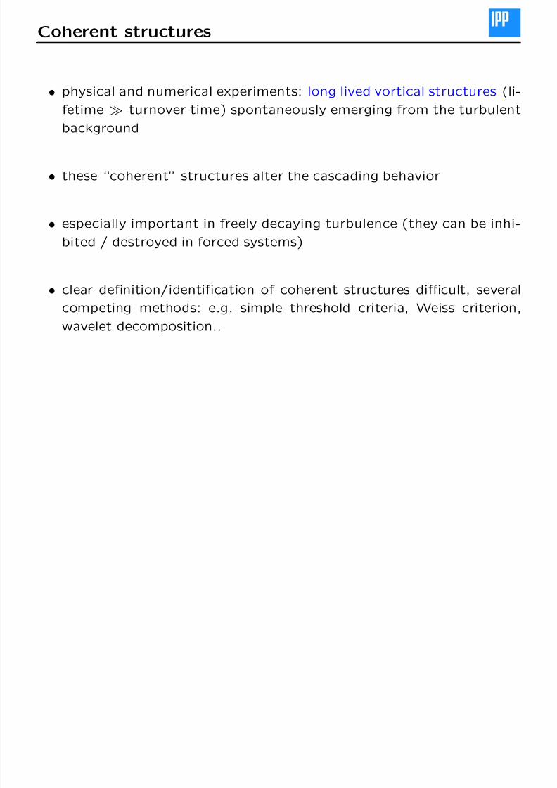
Coherent structures
• physical and numerical experiments: long lived vortical structures (li-
fetime turnover time) spontaneously emerging from the turbulent
background
• these “coherent” structures alter the cascading behavior
• especially important in freely decaying turbulence (they can be inhi-
bited / destroyed in forced systems)
• clear definition/identification of coherent structures difficult, several
competing methods: e.g. simple threshold criteria, Weiss criterion,
wavelet decomposition..
8/3/2019 2D Fluid Turbulence (Merz)
http://slidepdf.com/reader/full/2d-fluid-turbulence-merz 26/36
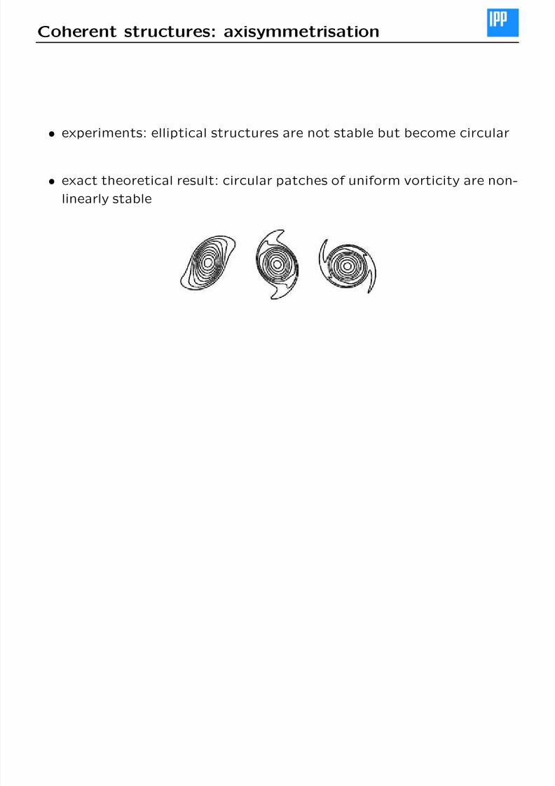
Coherent structures: axisymmetrisation
•experiments: elliptical structures are not stable but become circular
• exact theoretical result: circular patches of uniform vorticity are non-
linearly stable
8/3/2019 2D Fluid Turbulence (Merz)
http://slidepdf.com/reader/full/2d-fluid-turbulence-merz 27/36
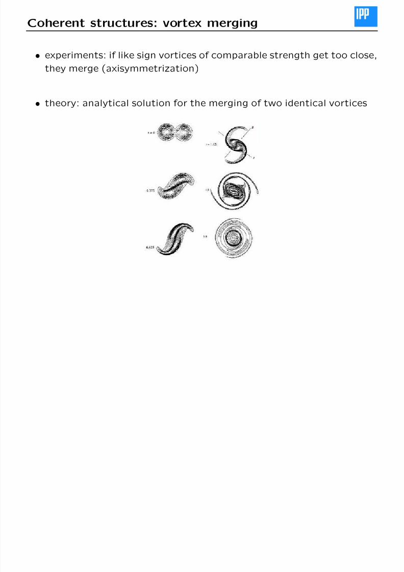
Coherent structures: vortex merging
• experiments: if like sign vortices of comparable strength get too close,they merge (axisymmetrization)
• theory: analytical solution for the merging of two identical vortices
8/3/2019 2D Fluid Turbulence (Merz)
http://slidepdf.com/reader/full/2d-fluid-turbulence-merz 28/36
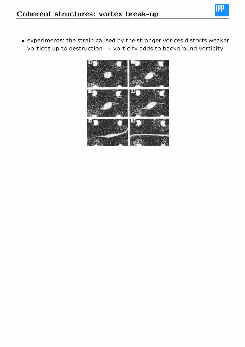
Coherent structures: vortex break-up
• experiments: the strain caused by the stronger vorices distorts weaker
vortices up to destruction → vorticity adds to background vorticity
C h t t t ti l ti
8/3/2019 2D Fluid Turbulence (Merz)
http://slidepdf.com/reader/full/2d-fluid-turbulence-merz 29/36
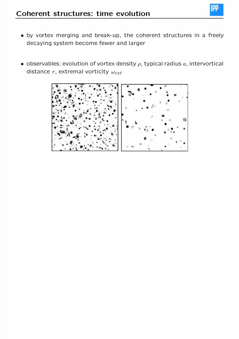
Coherent structures: time evolution
• by vortex merging and break-up, the coherent structures in a freely
decaying system become fewer and larger
• observables: evolution of vortex density ρ, typical radius a, intervortical
distance r, extremal vorticity ωext
’U i l d th ’ f dil t t
8/3/2019 2D Fluid Turbulence (Merz)
http://slidepdf.com/reader/full/2d-fluid-turbulence-merz 30/36
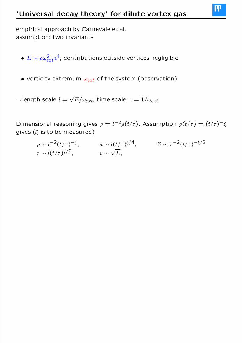
’Universal decay theory’ for dilute vortex gas
empirical approach by Carnevale et al.assumption: two invariants
•E ∼
ρω2
exta4, contributions outside vortices negligible
• vorticity extremum ωext of the system (observation)
→length scale l =√
E/ωext, time scale τ = 1/ωext
Dimensional reasoning gives ρ = l−2g(t/τ ). Assumption g(t/τ ) = (t/τ )−ξ
gives (ξ is to be measured)
ρ
∼l−2(t/τ )−ξ, a
∼l(t/τ )ξ/4, Z
∼τ −2(t/τ )−ξ/2
r ∼ l(t/τ )ξ/2, v ∼ √E,
’Uni ersal deca theor ’ comparison with DNS
8/3/2019 2D Fluid Turbulence (Merz)
http://slidepdf.com/reader/full/2d-fluid-turbulence-merz 31/36
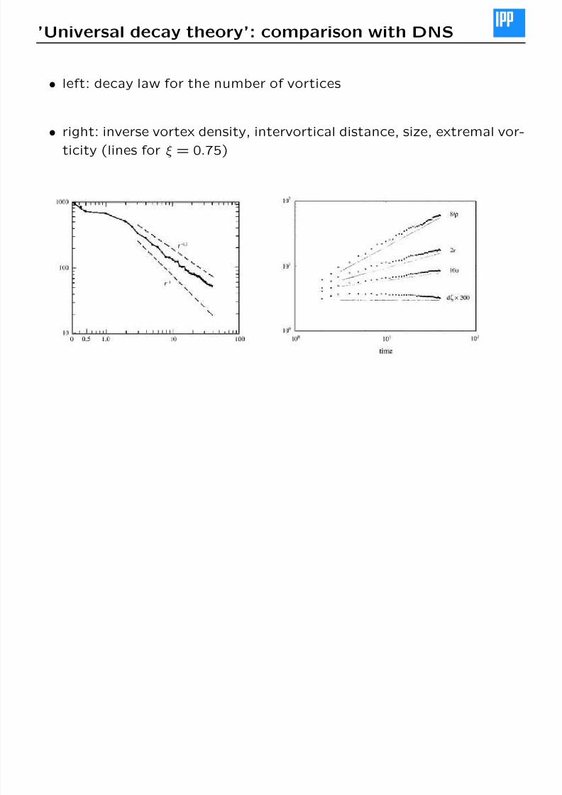
’Universal decay theory’: comparison with DNS
• left: decay law for the number of vortices
•right: inverse vortex density, intervortical distance, size, extremal vor-
ticity (lines for ξ = 0.75)
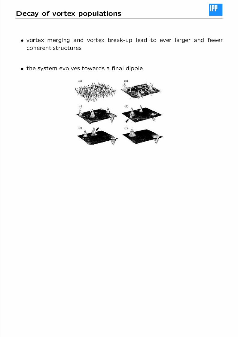
Decay of vortex populations
8/3/2019 2D Fluid Turbulence (Merz)
http://slidepdf.com/reader/full/2d-fluid-turbulence-merz 32/36
Decay of vortex populations
• vortex merging and vortex break-up lead to ever larger and fewer
coherent structures
• the system evolves towards a final dipole
Intermittency in 2D
8/3/2019 2D Fluid Turbulence (Merz)
http://slidepdf.com/reader/full/2d-fluid-turbulence-merz 33/36
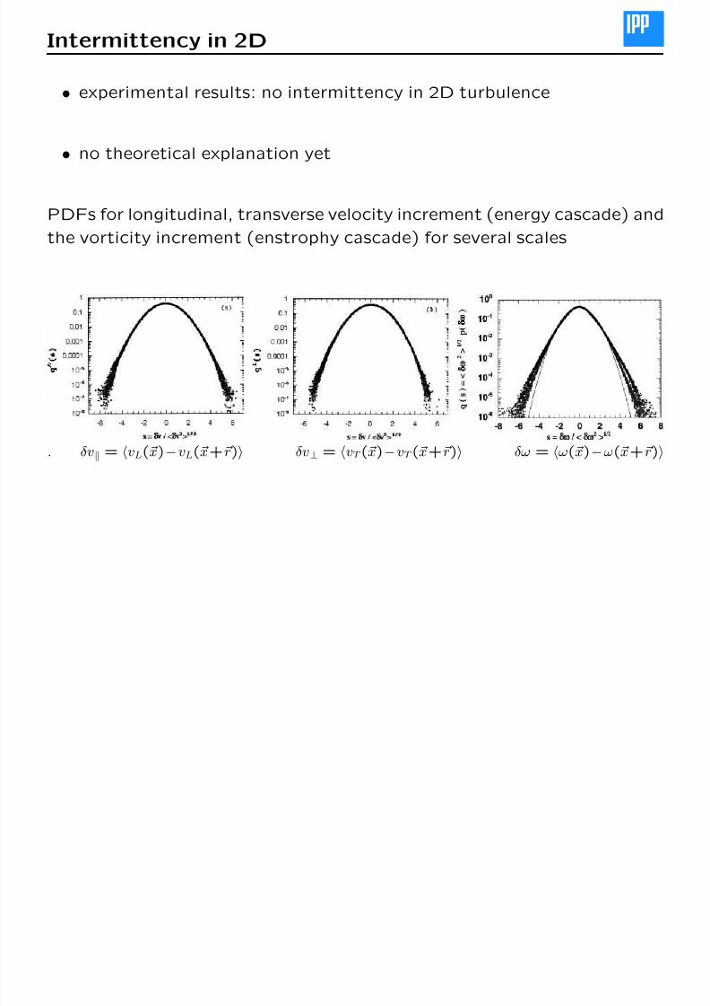
Intermittency in 2D
• experimental results: no intermittency in 2D turbulence
• no theoretical explanation yet
PDFs for longitudinal, transverse velocity increment (energy cascade) and
the vorticity increment (enstrophy cascade) for several scales
. δv = vL(x)−vL(x+r) δv⊥ = vT (x)−vT (x+r) δω = ω(x)−ω(x+r)
Intermittency in 2D
8/3/2019 2D Fluid Turbulence (Merz)
http://slidepdf.com/reader/full/2d-fluid-turbulence-merz 34/36
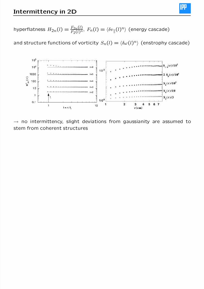
Intermittency in 2D
hyperflatness H 2n(l) = F 2n(l)F 2(l)n
, F n(l) = δv(l)n (energy cascade)
and structure functions of vorticity S n(l) = δω(l)n (enstrophy cascade)
→ no intermittency, slight deviations from gaussianity are assumed to
stem from coherent structures
Summary
8/3/2019 2D Fluid Turbulence (Merz)
http://slidepdf.com/reader/full/2d-fluid-turbulence-merz 35/36
Summary
• the existence of a dual enstrophy-energy cascade (KBL-theory) is
experimentally confirmed
• coherent structures play an important role (especially in decaying tur-
bulence) and modify the energy spectrum predicted by KBL-theory
• there is no intermittency found in experiments
• several systems of interest (e.g. geophysical flows, magnetized plas-mas) are approximately 2-dimensional - results of 2D fluid turbulence
are applicable
Further reading
8/3/2019 2D Fluid Turbulence (Merz)
http://slidepdf.com/reader/full/2d-fluid-turbulence-merz 36/36
Further reading
General 2D turbulence:
• P.A. Davidson, Turbulence, Oxford University Press (2004)
• M. Lesieur, Turbulence in Fluids, Kluwer (1997)
• U. Frisch, Turbulence, Cambridge University Press (1995)
• P. Tabelling, Two-dimensional turbulence: a physicist approach, Phys. Rep. 362,1-62 (2002)
Cascade classics
• Kraichnan, Inertial Ranges in Two-Dimensional Turbulence, Phys. Fluids 10, 1417(1967)
• Leith, Diffusion Approximation for Two-Dimensional Turbulence, Phys. Fluids 11,1612 (1968)
• Batchelor, Computation of the Energy Spectrum in Homogenous Two-Dimensional
Turbulence, Phys. Fluids 12, II-233 (1969)


![Dynamical modeling of sub-grid scales in 2D turbulencemasbu/dynmod.pdf · Dynamical modeling of sub-grid scales in 2D turbulence ... turbulence [2]. Yet another related approach in](https://static.fdocuments.net/doc/165x107/5b5f9ff67f8b9a553d8e9223/dynamical-modeling-of-sub-grid-scales-in-2d-turbulence-masbudynmodpdf-dynamical.jpg)


