2806 Neural ComputationRecurrent Neetworks

Lecture 12

2005 Ari Visa

Agenda

Some historical notes Some theory Recurrent networks Training Conclusions

Some Historical Notes

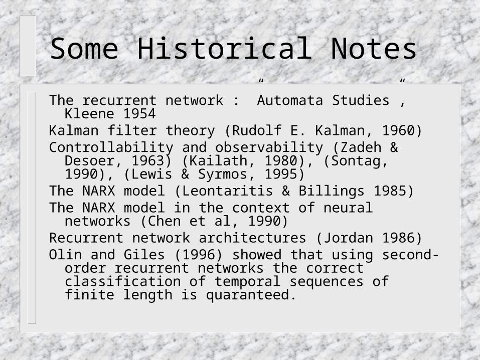
The recurrent network : ”Automata Studies”, Kleene 1954Kalman filter theory (Rudolf E. Kalman, 1960)Controllability and observability (Zadeh & Desoer, 1963)

(Kailath, 1980), (Sontag, 1990), (Lewis & Syrmos, 1995)The NARX model (Leontaritis & Billings 1985)The NARX model in the context of neural networks (Chen et

al, 1990) Recurrent network architectures (Jordan 1986)Olin and Giles (1996) showed that using second-order

recurrent networks the correct classification of temporal sequences of finite length is quaranteed.

Some Historical Notes

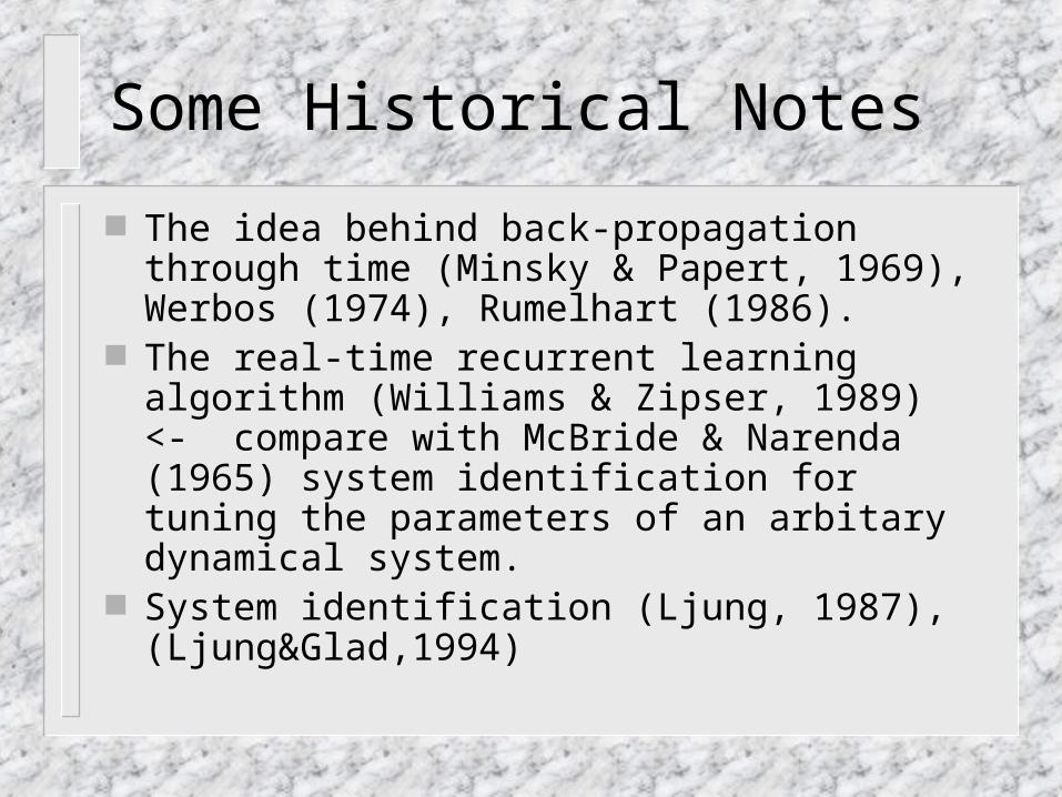
The idea behind back-propagation through time (Minsky & Papert, 1969), Werbos (1974), Rumelhart (1986).

The real-time recurrent learning algorithm (Williams & Zipser, 1989) <- compare with McBride & Narenda (1965) system identification for tuning the parameters of an arbitary dynamical system.

System identification (Ljung, 1987),(Ljung&Glad,1994)

Some Theory

Recurrent networks are neural networks with one or more feedback loops.

The feedback can be of a local or global kind. Input-output mapping networks, a recurrent network

responds temporally to an externally applied input signal → dynamically driven recurrent network.

The application of feedback enables recurrent network to acquire state representations, which make them suitable devices for such diverse applications as nonlinear prediction and modeling, adaptive equalization speech processing, plant control, automobile engine diagnostics.

Some Theory

Four specific network architectures will be represented.

They all incorporate a static multilayer perceptron or parts thereof.

They all exploit the nonlinear mapping capability of the multilayer perceptron.

Some Theory

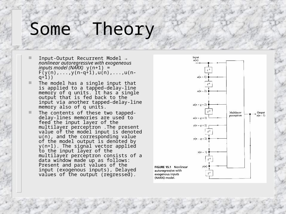
Input-Output Recurrent Model → nonlinear autoregressive with exogeneous inputs model (NARX) y(n+1) = F(y(n),...,y(n-q+1),u(n),...,u(n-q+1))

The model has a single input that is applied to a tapped-delay-line memory of q units. It has a single output that is fed back to the input via another tapped-delay-line memory also of q units.

The contents of these two tapped-delay-lines memories are used to feed the input layer of the multilayer perceptron .The present value of the model input is denoted u(n), and the corresponding value of the model output is denoted by y(n+1). The signal vector applied to the input layer of the multilayer perceptron consists of a data window made up as follows: Present and past values of the input (exogenous inputs), Delayed values of the output (regressed).

NARX

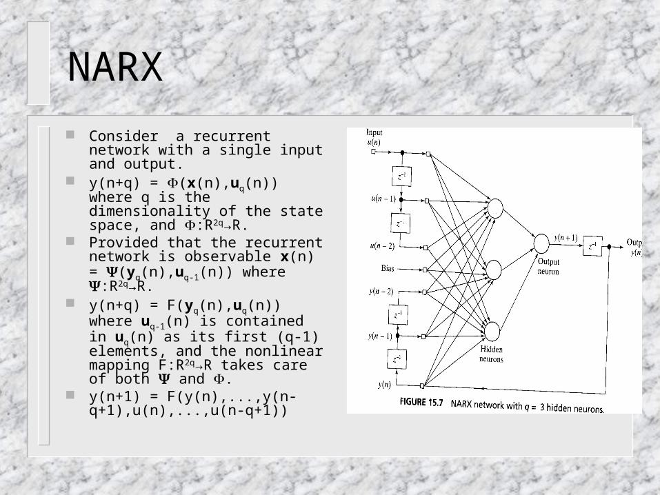
Consider a recurrent network with a single input and output.

y(n+q) = (x(n),uq(n)) where q is the dimensionality of the state space, and :R2q→R.

Provided that the recurrent network is observable x(n) = (yq(n),uq-

1(n)) where :R2q→R. y(n+q) = F(yq(n),uq(n)) where uq-

1(n) is contained in uq(n) as its first (q-1) elements, and the nonlinear mapping F:R2q→R takes care of both and .

y(n+1) = F(y(n),...,y(n-q+1),u(n),...,u(n-q+1))

Some Theory

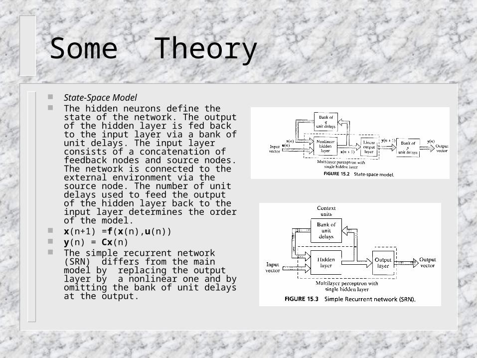
State-Space Model The hidden neurons define the state of

the network. The output of the hidden layer is fed back to the input layer via a bank of unit delays. The input layer consists of a concatenation of feedback nodes and source nodes. The network is connected to the external environment via the source node. The number of unit delays used to feed the output of the hidden layer back to the input layer determines the order of the model.

x(n+1) =f(x(n),u(n)) y(n) = Cx(n) The simple recurrent network (SRN)

differs from the main model by replacing the output layer by a nonlinear one and by omitting the bank of unit delays at the output.

State-Space Model

The state of a dynamical system is defined as a set of quantities that summarizes all the information about the past behavior of the system that is needed to uniquely describe its future behavior, except for the purely external effects arising from the applied input (excitation).

Let the q-by-1 vector x(n) denote the state of a nonlinear discrete-time system. Let the m-by-1 vector u(n) denote the input applied to the system, and the p-by-1 vector y(n) denote the corresponding output of the system.

The dynamic behavior of the system (noise free) is described. x(n+1) =(Wax(n)+Wbu(n)) (the process equation), y(n) = Cx(n) (the measurement equation) where Wa is a q-by-q matrix, Wb is a q-by-(m+1) matrix, C is a p-by-q matris; and : Rq→Rq is a diagonal map described by :[x1, x2,…, xq]T → [(x1), (x2),…, (xq)]T for some memoryless componen-wise nonlinearity : R→R .

The spaces Rm,Rq and Rp are called the input space, state space, and output space → m-input, p-output recurrent model of order q.

Some Theory

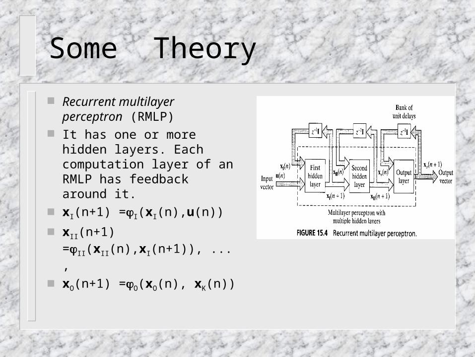
Recurrent multilayer perceptron (RMLP)

It has one or more hidden layers. Each computation layer of an RMLP has feedback around it.

xI(n+1) =I(xI(n),u(n))

xII(n+1) =II(xII(n),xI(n+1)), ...,

xO(n+1) =O(xO(n), xK(n))

Some Theory

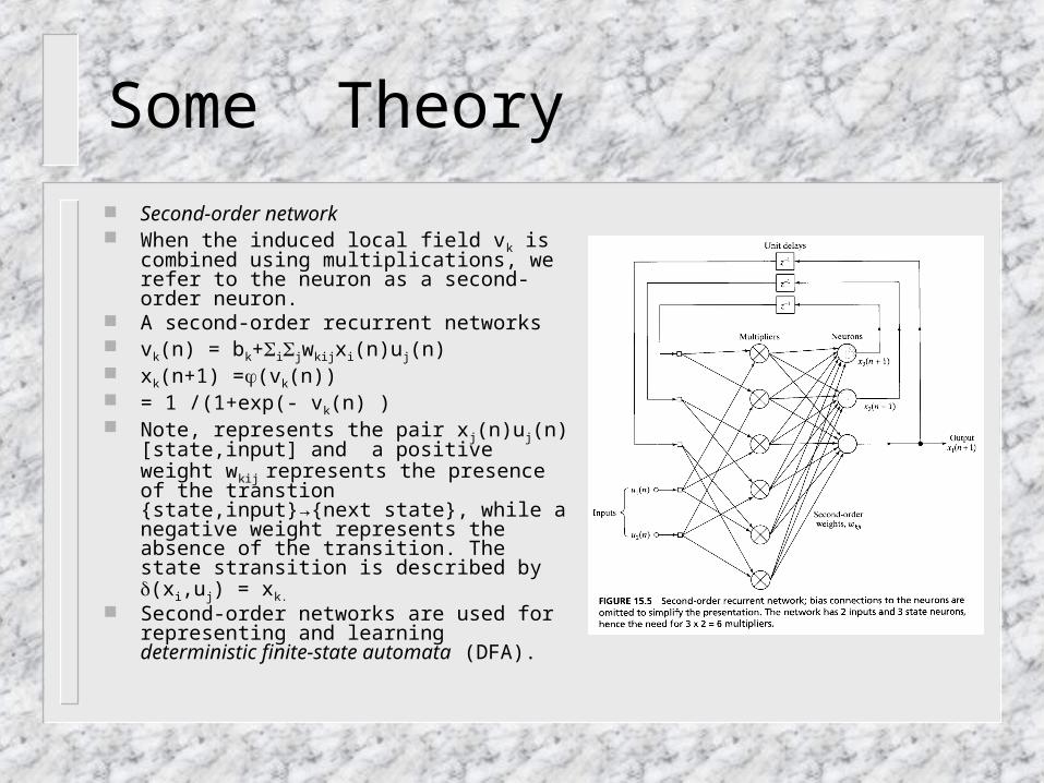
Second-order network When the induced local field vk is combined

using multiplications, we refer to the neuron as a second-order neuron.

A second-order recurrent networks vk(n) = bk+ijwkijxi(n)uj(n) xk(n+1) =(vk(n)) = 1 /(1+exp(- vk(n) ) Note, represents the pair xj(n)uj(n)

[state,input] and a positive weight wkij represents the presence of the transtion {state,input}→{next state}, while a negative weight represents the absence of the transition. The state stransition is described by (xi,uj) = xk.

Second-order networks are used for representing and learning deterministic finite-state automata (DFA).

Some Theory

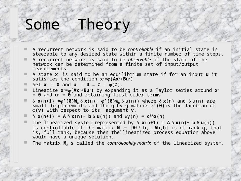
A recurrent network is said to be controllable if an initial state is steerable to any desired state within a finite number of time steps.

A recurrent network is said to be observable if the state of the network can be determined from a finite set of input/output measurements.

A state x- is said to be an equilibrium state if for an input u it satisfies the condition x-

=(Ax-+Bu-) Set x- = 0 and u- = 0 → 0 = (0). Linearize x-=(Ax-+Bu-) by expanding it as a Taylor series around x- = 0 and u- = 0 and

retaining first-order terms x(n+1) =’(0)Wa x(n)+ ’(0)wb u(n)) where x(n) and u(n) are small

displacements and the q-by-q matrix ’(0)is the Jacobian of (v) with respect to its argument v.

x(n+1) = A x(n)+ b u(n)) and y(n) = cTx(n) The linearized system represented by x(n+1) = A x(n)+ b u(n)) is controllable if the

matrix Mc = [Aq-1 b,…,Ab,b] is of rank q, that is, full rank, because then the linearized process equation above would have a unique solution.

The matrix Mc s called the controllability matrix of the linearized system.

Some Theory

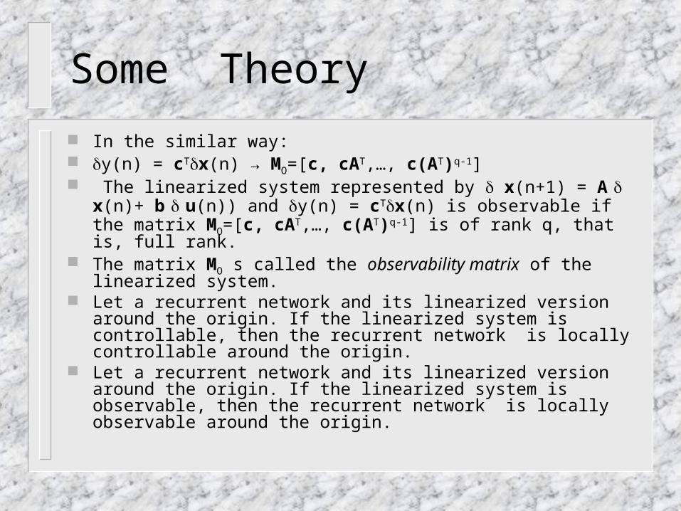
In the similar way: y(n) = cTx(n) → MO=[c, cAT,…, c(AT)q-1] The linearized system represented by x(n+1) = A x(n)+ b u(n))

and y(n) = cTx(n) is observable if the matrix MO=[c, cAT,…, c(AT)q-

1] is of rank q, that is, full rank. The matrix MO s called the observability matrix of the linearized

system. Let a recurrent network and its linearized version around the origin. If

the linearized system is controllable, then the recurrent network is locally controllable around the origin.

Let a recurrent network and its linearized version around the origin. If the linearized system is observable, then the recurrent network is locally observable around the origin.

Some Theory

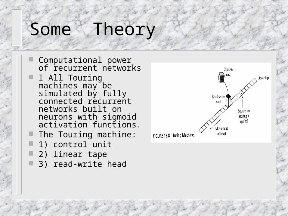
Computational power of recurrent networks

I All Touring machines may be simulated by fully connected recurrent networks built on neurons with sigmoid activation functions.

The Touring machine: 1) control unit 2) linear tape 3) read-write head

Some Theory

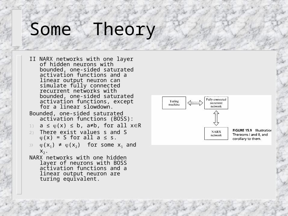
II NARX networks with one layer of hidden neurons with bounded, one-sided saturated activation functions and a linear output neuron can simulate fully connected recurrent networks with bounded, one-sided saturated activation functions, except for a linear slowdown.

Bounded, one-sided saturated activation functions (BOSS):

1) a ≤ (x) ≤ b, a≠b, for all xR2) There exist values s and S (x)

= S for all a ≤ s.3) (x1) ≠ (x2) for some x1 and x2.NARX networks with one hidden layer of

neurons with BOSS activation functions and a linear output neuron are turing equivalent.

Training

Epochwise training: For a given epoch, the recurrent network starts running from some initial state until it reaches a new state, at which point the training is stopped and the network is reset to an initial state for the next epoch.

Continuous training: this is suitable for situations where there are no reset states available and/or on-line learning is required. The network learns while signal processing is being performed by the network.

Training

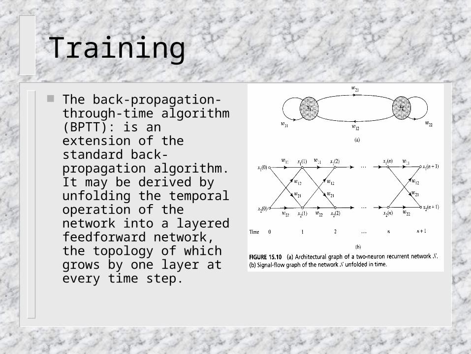
The back-propagation-through-time algorithm (BPTT): is an extension of the standard back-propagation algorithm. It may be derived by unfolding the temporal operation of the network into a layered feedforward network, the topology of which grows by one layer at every time step.

Training

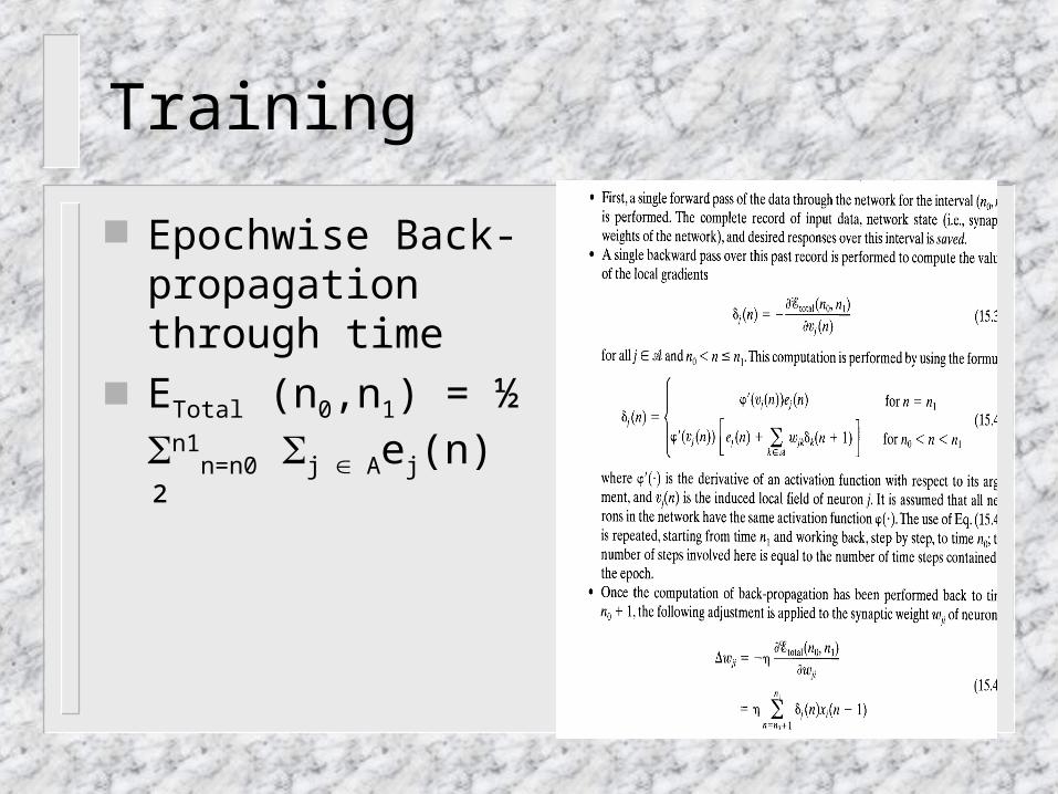
Epochwise Back-propagation through time

ETotal (n0,n1) = ½ n1n=n0

j Aej(n) ²

Training

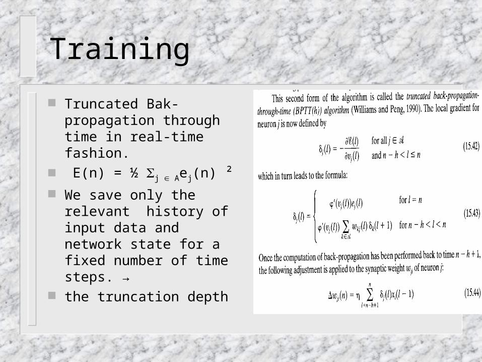
Truncated Bak-propagation through time in real-time fashion.

E(n) = ½ j Aej(n) ²

We save only the relevant history of input data and network state for a fixed number of time steps. →

the truncation depth

Training

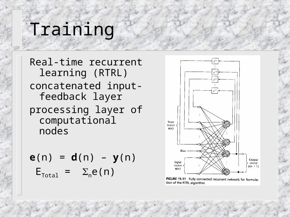
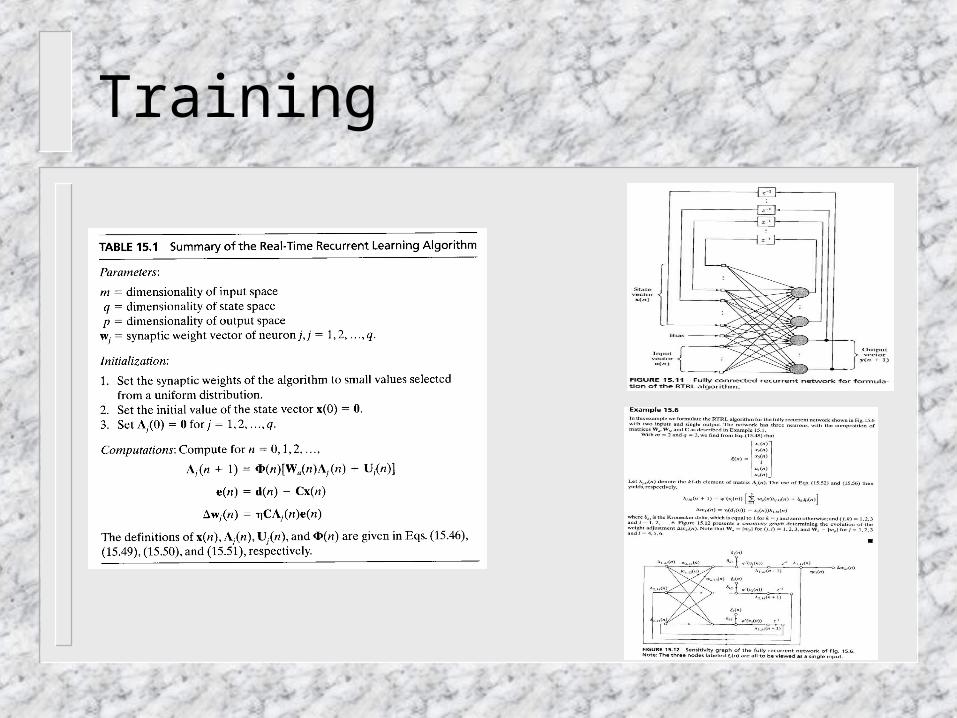
Real-time recurrent learning (RTRL)

concatenated input-feedback layer

processing layer of computational nodes

e(n) = d(n) – y(n)

ETotal = ne(n)

Training

Summary

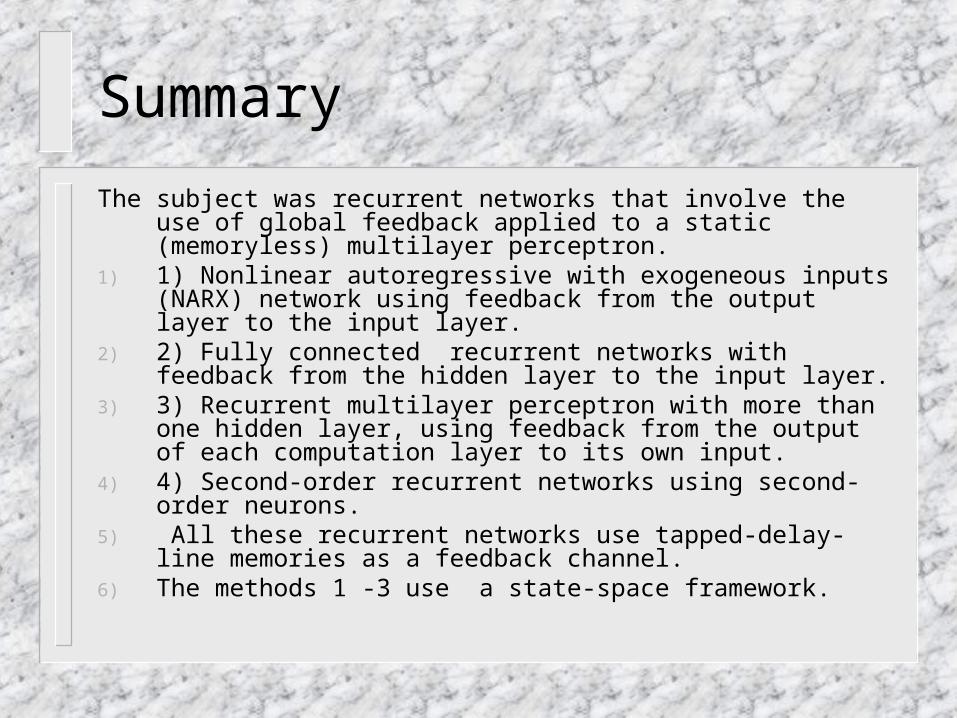
The subject was recurrent networks that involve the use of global feedback applied to a static (memoryless) multilayer perceptron.

1) 1) Nonlinear autoregressive with exogeneous inputs (NARX) network using feedback from the output layer to the input layer.

2) 2) Fully connected recurrent networks with feedback from the hidden layer to the input layer.

3) 3) Recurrent multilayer perceptron with more than one hidden layer, using feedback from the output of each computation layer to its own input.

4) 4) Second-order recurrent networks using second-order neurons.5) All these recurrent networks use tapped-delay-line memories as a

feedback channel.6) The methods 1 -3 use a state-space framework.

Summary

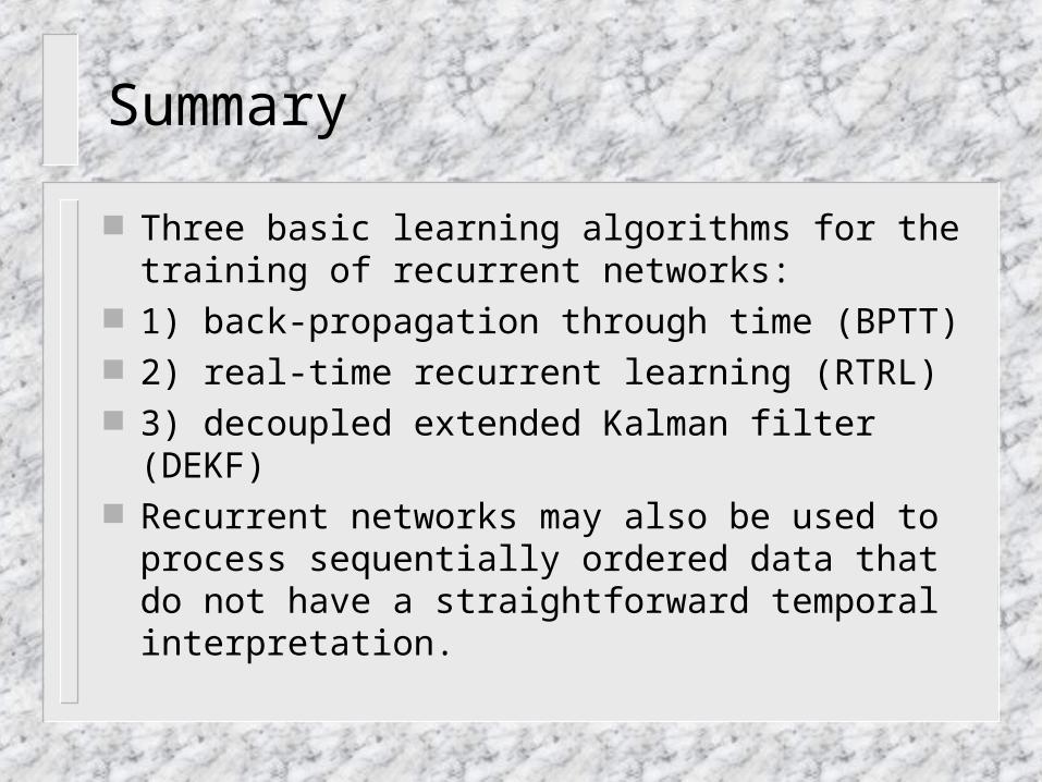
Three basic learning algorithms for the training of recurrent networks:

1) back-propagation through time (BPTT) 2) real-time recurrent learning (RTRL) 3) decoupled extended Kalman filter (DEKF) Recurrent networks may also be used to process

sequentially ordered data that do not have a straightforward temporal interpretation.