Heterogeneous Agent Models in Continuous TimePart II

Benjamin MollPrinceton

Rochester, 2 March 2017

January 24, 2018

OutlineLecture 1

1. Refresher: HJB equations2. Textbook heterogeneous agent model3. Numerical solution of HJB equations4. Models with non-convexities (Skiba)

Lecture 21. Analysis and numerical solution of heterogeneous agent model2. Transition dynamics/MIT shocks3. Stopping time problems4. Models with multiple assets (HANK)

“When Inequality Matters for Macro and Macro Matters for Inequality”1. Aggregate shocks via perturbation (Reiter)2. Application to consumption dynamics

1

Analysis and Numerical Solutionof Heterogeneous Agent Model

2

Recall Textbook Heterogeneous Agent Model

ρvj(a) = maxcu(c) + v ′j (a)(yj + ra − c) + λj(v−j(a)− vj(a)) (HJB)

0 = −d

da[sj(a)gj(a)]− λjgj(a) + λ−jg−j(a), (KF)

sj(a) = yj + ra − cj(a) = saving policy function from (HJB),∫ ∞a

(g1(a) + g2(a))da = 1, g1, g2 ≥ 0

S(r) :=

∫ ∞a

ag1(a)da +

∫ ∞a

ag2(a)da = B, B ≥ 0 (EQ)

• The two PDEs (HJB) and (KF) together with (EQ) fully characterizestationary equilibrium Derivation of (HJB) (KF)

3

Borrowing Constraints?

• Q: where is borrowing constraint a ≥ a in (HJB)?• A: “in” boundary condition

• Result: vj must satisfyv ′j (a) ≥ u′(yj + ra), j = 1, 2 (BC)

• Derivation:• the FOC still holds at the borrowing constraint

u′(cj(a)) = v′j (a) (FOC)

• for borrowing constraint not to be violated, needsj(a) = yj + ra − cj(a) ≥ 0 (∗)

• (FOC) and (∗)⇒ (BC).

• See slides on viscosity solutions for more rigorous discussionhttp://www.princeton.edu/~moll/viscosity_slides.pdf 4

Plan

• New theoretical results:

1. analytics: consumption, saving, MPCs of the poor

2. closed-form for wealth distribution with 2 income types

3. unique stationary equilibrium if IES ≥ 1 (sufficient condition)

Note: for 1. and 2. analyze partial equilibrium with r < ρ

• Computational algorithm:

• problems with non-convexities

• transition dynamics5

Result 1: Consumption, Saving Behavior of the Poor

Behavior near borrowing constraint depends on two factors1. tightness of constraint2. properties of u as c → 0

Assumption 1:As a→ a, coefficient of absolute risk aversion R(c) = −u′′(c)/u′(c)remains finite

R := − lima→a

u′′(y1 + ra)

u′(y1 + ra)<∞

• sufficient condition for A1: borrowing constraint is tighter than“natural borrowing constraint” a > −y1/r

• e.g. with CRRA utility

u(c) =c1−γ

1− γ ⇒ R =γ

y1 + ra

• but weaker: e.g. A1 satisfied with a = −y1/r and u(c) = −e−θc/θ6

Result 1: Consumption, Saving Behavior of the Poor

Rough version of Proposition: under A1 policy functions look like this

Wealth, a

Con

sumption

,c j(a)

a

c1(a)c2(a)

Wealth, aSav

ing,

sj(a)

a

s1(a)s2(a)

7

Result 1: Consumption, Saving Behavior of the Poor

Proposition: Assume r < ρ, y1 < y2 and that A1 holds. The solution to(HJB) has following properties:

1. s1(a) = 0 but s1(a) < 0 all a > a: only households exactly at theborrowing constraint are constrained

2. Saving and consumption policy functions close to a = a satisfys1(a) ∼ −

√2ν1√a − a

c1(a) ∼ y1 + ra +√2ν1√a − a

c ′1(a) ∼ r +1

2

√ν1

2(a − a)

ν1 =(ρ− r)u′(c1) + λ1(u′(c1)− u′(c2))

−u′′(c1)

Note: “f (a) ∼ g(a)” means lima→a f (a)/g(a) = 1, “f behaves like g close to a”8

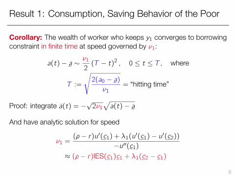
Result 1: Consumption, Saving Behavior of the Poor

Corollary: The wealth of worker who keeps y1 converges to borrowingconstraint in finite time at speed governed by ν1:

a(t)− a ∼ν12(T − t)2 , 0 ≤ t ≤ T , where

T :=

√2(a0 − a)ν1

= “hitting time”

Proof: integrate a(t) = −√2ν1√a(t)− a

And have analytic solution for speed

ν1 =(ρ− r)u′(c1) + λ1(u′(c1)− u′(c2))

−u′′(c1)≈ (ρ− r)IES(c1)c1 + λ1(c2 − c1)

9

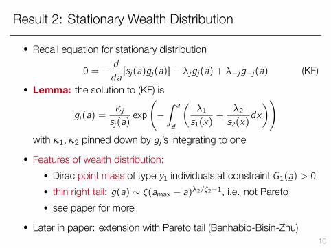
Result 2: Stationary Wealth Distribution

• Recall equation for stationary distribution

0 = −d

da[sj(a)gj(a)]− λjgj(a) + λ−jg−j(a) (KF)

• Lemma: the solution to (KF) is

gi(a) =κjsj(a)

exp

(−∫ aa

(λ1s1(x)

+λ2s2(x)

dx

))with κ1, κ2 pinned down by gj ’s integrating to one

• Features of wealth distribution:• Dirac point mass of type y1 individuals at constraint G1(a) > 0• thin right tail: g(a) ∼ ξ(amax − a)λ2/ζ2−1, i.e. not Pareto• see paper for more

• Later in paper: extension with Pareto tail (Benhabib-Bisin-Zhu)10

Result 2: Stationary Wealth Distribution

Wealth, a

Den

sities,gj(a)

a

g1(a)g2(a)

Note: in numerical solution, Dirac mass = finite spike in density 11

General Equilibrium: Existence and Uniqueness

Wealth, a

Sav

ing,

sj(a)

a

s1(a)s2(a)

Wealth, a

Den

sities,gj(a)

a

g1(a)g2(a)

12

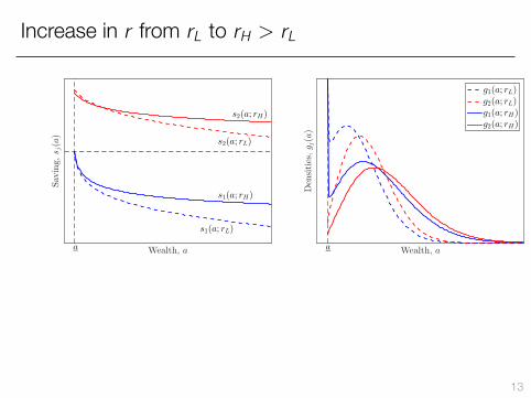
Increase in r from rL to rH > rL

Wealth, a

Sav

ing,

sj(a)

s1(a; rL)

s1(a; rH)

s2(a; rL)

s2(a; rH)

a Wealth, a

Den

sities,gj(a)

a

g1(a; rL)g2(a; rL)g1(a; rH)g2(a; rH)

13

Stationary Equilibrium

r

r = ρ

S(r)

B

a = a

Asset Supply S(r) =

∫ ∞a

ag1(a; r)da +

∫ ∞a

ag2(a; r)da

• Proposition: a stationary equilibrium exists• Proposition: if IES(c) ≥ 1 for all c and no borrowing a ≥ 0,

stationary equilibrium is unique 14

Computations forHeterogeneous Agent Model

15

Computations for Heterogeneous Agent Model

• Hard part: HJB equation. But already know how to do that.• Easy part: KF equation. Once you solved HJB equation, get KF

equation “for free”• System to be solved

ρv1(a) = maxcu(c) + v ′1(a)(y1 + ra − c) + λ1(v2(a)− v1(a))

ρv2(a) = maxcu(c) + v ′2(a)(y2 + ra − c) + λ2(v1(a)− v2(a))

0 = −d

da[s1(a)g1(a)]− λ1g1(a) + λ2g2(a)

0 = −d

da[s2(a)g2(a)]− λ2g2(a) + λ1g1(a)

1 =

∫ ∞a

g1(a)da +

∫ ∞a

g2(a)da

0 =

∫ ∞a

ag1(a)da +

∫ ∞a

ag2(a)da ≡ S(r)16

Computations for Heterogeneous Agent Model

• As before, discretized HJB equation is

ρv = u(v) + A(v)v (HJBd)

• A is N × N transition matrix

• here N = 2× I, I=number of wealth grid points• A depends on v (nonlinear problem)• solve using implicit scheme

17

Visualization of A (output of spy(A) in Matlab)

0 10 20 30 40 50 60

0

10

20

30

40

50

60

nz = 177 18

Computing the FK Equation

• Equations to be solved

0 = −d

da[s1(a)g1(a)]− λ1g1(a) + λ2g2(a)

0 = −d

da[s2(a)g2(a)]− λ2g2(a) + λ1g1(a)

with 1 =∫∞a g1(a)da +

∫∞a g2(a)da

• Actually, super easy: discretized version is simply0 = A(v)Tg (KFd)

• eigenvalue problem• get KF for free, one more reason for using implicit scheme

• Why transpose?• operator in (HJB) is “adjoint” of operator in (KF)• “adjoint” = infinite-dimensional analogue of matrix transpose

• In principle, can use similar strategy in discrete time19

Finding the Equilibrium Interest Rate

Use bisection method• increase r whenever S(r) < B• decrease r whenever S(r) > B

r

r = ρ

S(r)

B

a = a

20

A Model with a Continuum of Income Types

• Assume idiosyncratic income follows diffusion processdyt = µ(yt)dt + σ(yt)dWt

• Reflecting barriers at y and yρv(a, y) = max

cu(c) + ∂av(a, y)(y + ra − c) + µ(y)∂yv(a, y) +

σ2(y)

2∂yyv(a, y)

0 = −∂a[s(a, y)g(a, y)]− ∂y [µ(y)g(a, y)] +1

2∂yy [σ

2(y)g(a, y)]

1 =

∫ ∞0

∫ ∞a

g(a, y)dady

0 =

∫ ∞0

∫ ∞a

ag(a, y)dady =: S(r)

• Borrowing constraint: ∂av(a, y) ≥ u′(y + ra), all y• reflecting barriers (see e.g. Dixit “Art of Smooth Pasting”)

0 = ∂yv(a, y) = ∂yv(a, y)21

It doesn’t matter whether you solve ODEs or PDEs⇒ everything generalizes

http://www.princeton.edu/~moll/HACTproject/huggett_diffusion_partialeq.m

22

Visualization of A (output of spy(A) in Matlab)

nz = 157490 500 1000 1500 2000 2500 3000 3500 4000

0

500

1000

1500

2000

2500

3000

3500

4000

23

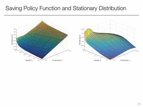
Saving Policy Function and Stationary Distribution

1.5

Productivity, z

1

0.525

20

Wealth, a

15

10

5

0

-0.4

-0.2

-0.8

0

0.6

0.4

0.2

-0.6

Sav

ings

s(a

,z)

1.5

Productivity, z

1

0.58

6

Wealth, a

4

2

0

0.05

0.1

0

0.15

0.2

0.25

Den

sity

g(a

,z)

24

Summary: Stationary Equilibrium

• Can always write as

ρv = u(v) + A(v,p)v

0 = A(v,p)Tg

0 = F(p,g)

where p is a vector of prices.

25

Accuracy of Finite Difference Method

26

Accuracy of Finite Difference Method?

Two experiments:

1. special case: comparison with closed-form solution

2. general case: comparison with numerical solution computed usingvery fine grid

27

Accuracy of Finite Difference Method, Experiment 1• see http://www.princeton.edu/~moll/HACTproject/HJB_accuracy1.m

• Achdou et al. (2017) get closed-form solution if• exponential utility u′(c) = c−θc• no income risk and r = 0 so that a = y − c (and a ≥ 0)⇒ s(a) = −

√2νa, c(a) = y +

√2νa, ν :=

ρ

θ• Accuracy with I = 1000 grid points (c(a) = numerical solution)

Wealth a

0 0.2 0.4 0.6 0.8 1

Con

sumption

0.1

0.15

0.2

0.25

0.3

0.35

0.4

0.45

Closed-form solution c(a)Numerical solution, c(a)

Wealth, a0 0.2 0.4 0.6 0.8 1

Percentage

Error,100×(c(a)−c(a))/c(a)

-0.4

-0.35

-0.3

-0.25

-0.2

-0.15

-0.1

-0.05

0

0.05

28

Accuracy of Finite Difference Method, Experiment 1• see http://www.princeton.edu/~moll/HACTproject/HJB_accuracy1.m

• Achdou et al. (2017) get closed-form solution if• exponential utility u′(c) = c−θc• no income risk and r = 0 so that a = y − c (and a ≥ 0)⇒ s(a) = −

√2νa, c(a) = y +

√2νa, ν :=

ρ

θ• Accuracy with I = 30 grid points (c(a) = numerical solution)

Wealth a

0 0.2 0.4 0.6 0.8 1

Con

sumption

0.1

0.15

0.2

0.25

0.3

0.35

0.4

0.45

Closed-form solution c(a)Numerical solution, c(a)

Wealth, a0 0.2 0.4 0.6 0.8 1

Percentage

Error,100×(c(a)−c(a))/c(a)

-0.4

-0.35

-0.3

-0.25

-0.2

-0.15

-0.1

-0.05

0

0.05

29

Accuracy of Finite Difference Method, Experiment 2• see http://www.princeton.edu/~moll/HACTproject/HJB_accuracy2.m

• Consider HJB equation with continuum of income typesρv(a, y) = max

cu(c)+∂av(a, y)(y+ra−c)+µ(y)∂yv(a, y)+σ

2(y)2 ∂yyv(a, y)

• Compute twice:1. with very fine grid: I = 3000 wealth grid points2. with coarse grid: I = 300 wealth grid points

then examine speed-accuracy tradeoff (accuracy = error in agg C)Speed (in secs) Aggregate C

I = 3000 0.916 1.1541I = 300 0.076 1.1606

row 2/row 1 0.0876 1.005629• i.e. going from I = 3000 to I = 300 yields > 10× speed gain and0.5% reduction in accuracy (but note: even I = 3000 very fast)

• Other comparisons? Feel free to play around with HJB_accuracy2.m 30

Transition Dynamics/MIT Shocks

31

Transition Dynamics

Do Aiyagari version of the model

r(t) =FK(K(t), 1)− δ, w(t) = FL(K(t), 1) (P)

K(t) =

∫ag1(a, t)da +

∫ag2(a, t)da (K)

ρvj(a, t) =maxcu(c) + ∂avj(a, t)(w(t)zj + r(t)a − c)

+ λj(v−j(a, t)− vj(a, t)) + ∂tvj(a, t),(HJB)

∂tgj(a, t) =− ∂a[sj(a, t)gj(a, t)]− λjgj(a, t) + λ−jg−j(a, t), (KF)

sj(a, t) =w(t)zj + r(t)a − cj(a, t), cj(a, t) = (u′)−1(∂avj(a, t))

• Given initial condition gj,0(a), the two PDEs (HJB) and (KF)together with (P) and (K) fully characterize equilibrium.

32

Transition Dynamics

• Recall discretized equations for stationary equilibriumρv = u(v) + A(v)v

0 = A(v)Tg

• Transition dynamics• denote vni,j = vj(ai , tn) and stack into vn• denote gni,j = gj(ai , tn) and stack into gn

ρvn = u(vn+1) + A(vn+1)vn +1

∆t(vn+1 − vn)

gn+1 − gn

∆t= A(vn)Tgn+1

• Terminal condition for v: vN = v∞ (steady state)• Initial condition for g: g1 = g0.

33

Transition Dynamics

• (HJB) looks forward, runs backwards in time

• (KF) looks backward, runs forward in time

• Algorithm: Guess K0(t) and then for ℓ = 0, 1, 2, ...

1. find prices r ℓ(t) and w ℓ(t)2. solve (HJB) backwards in time given terminal cond’n vj,∞(a)3. solve (KF) forward in time given given initial condition gj,0(a)4. Compute Sℓ(t) =

∫agℓ1(a, t)da +

∫agℓ2(a, t)da

5. Update Kℓ+1(t) = (1− ξ)Kℓ(t) + ξSℓ(t) where ξ ∈ (0, 1] is arelaxation parameter

34

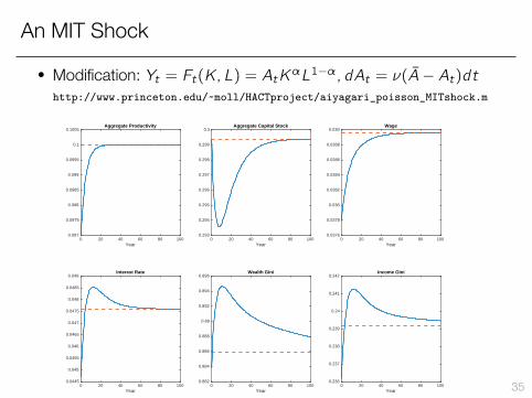
An MIT Shock

• Modification: Yt = Ft(K,L) = AtKαL1−α, dAt = ν(A− At)dthttp://www.princeton.edu/~moll/HACTproject/aiyagari_poisson_MITshock.m

Year0 20 40 60 80 100

0.097

0.0975

0.098

0.0985

0.099

0.0995

0.1

0.1005Aggregate Productivity

Year0 20 40 60 80 100

0.293

0.294

0.295

0.296

0.297

0.298

0.299

0.3Aggregate Capital Stock

Year0 20 40 60 80 100

0.0376

0.0378

0.038

0.0382

0.0384

0.0386

0.0388

0.039Wage

Year0 20 40 60 80 100

0.0445

0.045

0.0455

0.046

0.0465

0.047

0.0475

0.048

0.0485

0.049Interest Rate

Year0 20 40 60 80 100

0.882

0.884

0.886

0.888

0.89

0.892

0.894

0.896Wealth Gini

Year0 20 40 60 80 100

0.236

0.237

0.238

0.239

0.24

0.241

0.242Income Gini

35

Stopping Time Problems

36

Stopping Time Problems• In lots of problems in economics, agents have to choose an

optimal stopping time• Quite often these problems entail some form of non-convexity• Examples:

• how long should a low productivity firm wait before it exits anindustry?

• how long should a firm wait before it resets its prices?• when should you exercise an option?• etc... Stokey’s book is all about these kind of problems

• These problems are very awkward in discrete time because yourun into integer problems

• Big payoff from working in continuous time• Next: flexible algorithm for solving such problems, also works if

don’t have simple threshold rules and with states > 1 37

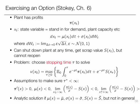
Exercising an Option (Stokey, Ch. 6)• Plant has profits

π(xt)

• xt : state variable = stand in for demand, plant capacity etcdxt = µ(xt)dt + σ(xt)dWt

where dWt := lim∆t→0 ε√∆t, ε ∼ N (0, 1)

• Can shut down plant at any time, get scrap value S(xt), butcannot reopen

• Problem: choose stopping time τ to solve

v(x0) = maxτ≥0

{E0∫ τ0

e−ρtπ(xt)dt + e−ρτS(xτ )

}• Assumptions to make sure τ∗ <∞:

π′(x) > 0, µ(x) < 0, limx↓−∞

(π(x)ρ − S(x)

)< 0, lim

x↑+∞

(π(x)ρ − S(x)

)> 0

• Analytic solution if µ(x) = µ, σ(x) = σ, S(x) = S, but not in general38

Exercising an Option: Standard Approach

• Assume scrap value is independent of x : S(x) = S• Optimal policy = threshold rule: exit if xt falls below x

• Standard approach (see e.g. Stokey, Ch.6):

ρv(x) = π(x) + µ(x)v ′(x) +σ2(x)

2v ′′(x), x > x

with “value matching” and “smooth pasting” at x :

v(x) = S, v ′(x) = 0

• but things more complicated if S depends on x or if dimension > 1• ⇒ can’t use threshold property• want algorithm that works also in those cases

39

Exercising an Option: HJBVI Approach• Denote X = set of x such that don’t exit:x ∈ X : v(x)≥S(x), ρv(x) = π(x) + µ(x)v ′(x) + σ

2(x)2 v

′′(x)

x ∈ X : v(x) = S(x), ρv(x)≥π(x) + µ(x)v ′(x) + σ2(x)2 v

′′(x)

• Can write compactly as:

min

{ρv(x)− π(x)− µ(x)v ′(x)−

σ2(x)

2v ′′(x), v(x)− S(x)

}= 0 (∗)

• Note: have used that following two statements are equivalent1. for all x , either f (x) ≥ 0, g(x) = 0 or f (x) = 0, g(x) ≥ 02. min{f (x), g(x)} = 0 for all x

• (∗) is called “HJB variational inequality” (HJBVI)• Important: did not impose smooth pasting

• instead, it’s a result: if S, can prove that (∗) implies v ′(x) = 0• see e.g. Oksendal http://th.if.uj.edu.pl/~gudowska/dydaktyka/Oksendal.pdf (who

calls “smooth pasting” “high contact (or smooth fit) principle”) 40

Finite Difference Scheme for solving HJBVI

• Codeshttp://www.princeton.edu/~moll/HACTproject/option_simple_LCP.m,http://www.mathworks.com/matlabcentral/fileexchange/20952

• Main insight: discretized HJBVI = Linear Complementarity Problem(LCP) https://en.wikipedia.org/wiki/Linear_complementarity_problem

• Prototypical LCP: given matrix B and vector q, find z such thatz ′(Bz + q) = 0

z ≥ 0Bz + q ≥ 0

• There are many good LCP solvers in Matlab and other languages

• Best one I’ve found if B large but sparse (Newton-based):http://www.mathworks.com/matlabcentral/fileexchange/20952

41

Finite Difference Scheme for solving HJBVI• Recall HJBVI

min

{ρv(x)− π(x)− µ(x)v ′(x)−

σ2(x)

2v ′′(x), v(x)− S(x)

}= 0

• Without exit, discretize as

ρvi = πi + µi(vi)′ +σ2i2(vi)

′′ ⇔ ρv = π + Av

• With exit:min{ρv − π − Av , v − S} = 0

• Equivalently:(v − S)′(ρv − π − Av) = 0

v ≥ Sρv − π − Av ≥ 0

• But this is just an LCP with z = v − S, B = ρI− A, q = −π + B!!42

Generalization: Menu Cost Model

• Work in progress: menu cost model (Golosov-Lucas) via HJBVI

• HANK + menu cost model + aggregate shocks

43

Multiple Assets

44

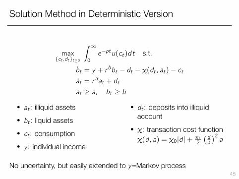
Solution Method in Deterministic Version

max{ct ,dt}t≥0

∫ ∞0

e−ρtu(ct)dt s.t.

bt = y + rbbt − dt − χ(dt , at)− ct

at = raat + dt

at ≥ a, bt ≥ b

• at : illiquid assets• bt : liquid assets• ct : consumption• y : individual income

• dt : deposits into illiquidaccount

• χ: transaction cost functionχ(d, a) = χ0|d |+ χ12

(da

)2a

No uncertainty, but easily extended to y=Markov process45

How to “upwind” with two endogenous states• HJB equation

ρv(a, b) = maxcu(c) + ∂bv(a, b)(y + r

bb − d − χ(d, a)− c)

+ ∂av(a, b)(d + raa)

• FOC for d : (1 + χd(d, a))∂bv = ∂av

⇒ d =

(∂av

∂bv− 1 + χ0

)− aχ1+

(∂av

∂bv− 1− χ0

)+ aχ1

• Applying standard upwind scheme

ρvi ,j = u(ci) +vi+1,j − vi ,j∆b

(sbi,j)+ +vi ,j − vi−1,j∆b

(sbi,j)+

+vi ,j+1 − vi ,j∆a

(sai,j)+ +vi ,j − vi ,j−1∆a

(sai,j)−

where e.g. sbi,j = y + rbbi − di ,j − χ(di ,j , aj)− ci ,j• Hard: di ,j depends on forward/backward choice for ∂bvi ,j , ∂avi ,j

46

How to “upwind” with two endogenous states

• Convenient trick: “splitting the drift”ρv(a, b) = max

cu(c) + ∂bv(a, b)(y + r

bb − c)

+ ∂bv(a, b)(−d − χ(d, a))+ ∂av(a, b)d

+ ∂av(a, b)raa

and upwind each term separately• Can check this satisfies Barles-Souganidis monotonicity condition• For an application, see

http://www.princeton.edu/~moll/HACTproject/two_asset_kinked.pdf

http://www.princeton.edu/~moll/HACTproject/two_asset_kinked.m

Subroutineshttp://www.princeton.edu/~moll/HACTproject/two_asset_kinked_cost.m

http://www.princeton.edu/~moll/HACTproject/two_asset_kinked_FOC.m47