24. Eigenvectors, spectral theorems

24. Eigenvectors, spectral theorems

24.1 Eigenvectors, eigenvalues24.2 Diagonalizability, semi-simplicity24.3 Commuting operators ST = TS24.4 Inner product spaces24.5 Projections without coordinates24.6 Unitary operators24.7 Corollaries of the spectral theorem24.8 Spectral theorems24.9 Worked examples

1. Eigenvectors, eigenvalues

Let k be a field, not necessarily algebraically closed.

Let T be a k-linear endomorphism of a k-vectorspace V to itself, meaning, as usual, that

T (v + w) = Tv + TW and T (cv) = c · Tv

for v, w ∈ V and c ∈ k. The collection of all such T is denoted Endk(V ), and is a vector space over k withthe natural operations

(S + T )(v) = Sv + Tv (cT )(v) = c · Tv

A vector v ∈ V is an eigenvector for T with eigenvalue c ∈ k if

T (v) = c · v

or, equivalently, if(T − c · idV ) v = 0

A vector v is a generalized eigenvector of T with eigenvalue c ∈ k if, for some integer ` ≥ 1

(T − c · idV )` v = 0

337

338 Eigenvectors, spectral theorems

We will often suppress the idV notation for the identity map on V , and just write c for the scalar operatorc · idV . The collection of all λ-eigenvectors for T is the λ-eigenspace for T on V , and the collection of allgeneralized λ-eigenvectors for T is the generalized λ-eigenspace for T on V .

[1.0.1] Proposition: Let T ∈ Endk(V ). For fixed λ ∈ k the λ-eigenspace is a vector subspace of V . Thegeneralized λ-eigenspace is also a vector subspace of V . And both the λ-eigenspace and the generalized oneare stable under the action of T .

Proof: This is just the linearity of T , hence, of T − λ. Indeed, for v, w λ-eigenvectors, and for c ∈ k,

T (v + w) = Tv + TW = λv + λw = λ(v + w) and T (cv) = c · Tv = c · λv = lam · cv

If (T − λ)mv = 0 and (T − λ)nw = 0, let N = max(m,n). Then

(T − λ)N (v + w) = (T − λ)Nv + (T − λ)Nw = (T − λ)N−m(T − λ)mv + (T − λ)N−n(T − λ)nw

= (T − λ)N−m0 + (T − λ)N−n0 = 0

Similarly, generalized eigenspaces are stable under scalar multiplication.

Since the operator T commutes with any polynomial in T , we can compute, for (T − λ)nv = 0,

(T − λ)n(Tv) = T · (T − λ)n(v) = T (0) = 0

which proves the stability. ///

[1.0.2] Proposition: Let T ∈ Endk(V ) and let v1, . . . , vm be eigenvectors for T , with distinct respectiveeigenvalues λ1, . . . , λm in k. Then for scalars ci

c1v1 + . . .+ cmvm = 0 =⇒ all ci = 0

That is, eigenvectors for distinct eigenvalues are linearly independent.

Proof: Suppose that the given relation is the shortest such with all ci 6= 0. Then apply T − λ1 to therelation, to obtain

0 + (λ2 − λ1)c2v2 . . .+ (λm − λ1)cmvm = 0 =⇒ all ci = 0

For i > 1 the scalars λi − λ1 are not 0, and (λi − λ1)vi is again a non-zero λi-eigenvector for T . Thiscontradicts the assumption that the relation was the shortest. ///

So far no use was made of finite-dimensionality, and, indeed, all the above arguments are correct withoutassuming finite-dimensionality. Now, however, we need to assume finite-dimensionality. In particular,

[1.0.3] Proposition: Let V be a finite-dimensional vector space over k. Then

dimk Endk(V ) = (dimk V )2

In particular, Endk(V ) is finite-dimensional.

Garrett: Abstract Algebra 339

Proof: An endomorphism T is completely determined by where it sends all the elements of a basis v1, . . . , vnof V , and each vi can be sent to any vector in V . In particular, let Eij be the endomorphism sending vi tovj and sending v` to 0 for ` 6= i. We claim that these endomorphisms are a k-basis for Endk(V ). First, theyspan, since any endomorphism T is expressible as

T =∑ij

cijEij

where the cij ∈ k are determined by the images of the given basis

T (vi) =∑j

cijvj

On the other hand, suppose for some coefficients cij∑ij

cij Eij = 0 ∈ Endk(V )

Applying this endomorphism to vi gives ∑j

cijvj = 0 ∈ V

Since the vj are linearly independent, this implies that all cij are 0. Thus, the Eij are a basis for the spaceof endomorphisms, and we have the dimension count. ///

For V finite-dimensional, the homomorphism

k[x] −→ k[T ] ⊂ Endk(V ) by x −→ T

from the polynomial ring k[x] to the ring k[T ] of polynomials in T must have a non-trivial kernel, since k[x]is infinite-dimensional and k[T ] is finite-dimensional. The minimal polynomial f(x) ∈ k[x] of T is the(unique) monic generator of that kernel.

[1.0.4] Proposition: The eigenvalues of a k-linear endomorphism T are exactly the zeros of its minimalpolynomial. [1]

Proof: Let f(x) be the minimal polynomial. First, suppose that x − λ divides f(x) for some λ ∈ k, andput g(x) = f(x)/(x − λ). Since g(x) is not divisible by the minimal polynomial, there is v ∈ V such thatg(T )v 6= 0. Then

(T − λ) · g(T )v = f(T ) · v = 0

so g(T )v is a (non-zero) λ-eigenvector of T . On the other hand, suppose that λ is an eigenvalue, and let vbe a non-zero λ-eigenvector for T . If x − λ failed to divide f(x), then the gcd of x − λ and f(x) is 1, andthere are polynomials a(x) and b(x) such that

1 = a · (x− λ) + b · f

Mapping x −→ T givesidV = a(T )(T − λ) + 0

Applying this to v givesv = a(T )(T − λ)(v) = a(T ) · 0 = 0

which contradicts v 6= 0. ///

[1] This does not presume that k is algebraically closed.


[1.0.5] Corollary: Let k be algebraically closed, and V a finite-dimensional vector space over k. Thenthere is at least one eigenvalue and (non-zero) eigenvector for any T ∈ Endk(V ).

Proof: The minimal polynomial has at least one linear factor over an algebraically closed field, so by theprevious proposition has at least one eigenvector. ///

[1.0.6] Remark: The Cayley-Hamilton theorem [2] is often invoked to deduce the existence of at leastone eigenvector, but the last corollary shows that this is not necessary.

2. Diagonalizability, semi-simplicity

A linear operator T ∈ Endk(V ) on a finite-dimensional vector space V over a field k is diagonalizable [3] ifV has a basis consisting of eigenvectors of T . Equivalently, T may be said to be semi-simple, or sometimesV itself, as a k[T ] or k[x] module, is said to be semi-simple.

Diagonalizable operators are good, because their effect on arbitrary vectors can be very clearly describedas a superposition of scalar multiplications in an obvious manner, namely, letting v1, . . . , vn be eigenvectorswith eigenvalues λ1, . . . , λn, if we manage to express a given vector v as a linear combination [4]

v = c1v1 + . . .+ cnvn

of the eigenvectors vi, with ci ∈ k, then we can completely describe the effect of T , or even iterates T `, onv, by

T `v = λ`1 · c1v1 + . . .+ λ`n · cnvn

[2.0.1] Remark: Even over an algebraically closed field k, an endomorphism T of a finite-dimensionalvector space may fail to be diagonalizable by having non-trivial Jordan blocks, meaning that some one ofits elementary divisors has a repeated factor. When k is not necessarily algebraically closed, T may fail tobe diagonalizable by having one (hence, at least two) of the zeros of its minimal polynomial lie in a properfield extension of k. For not finite-dimensional V , there are further ways that an endomorphism may fail tobe diagonalizable. For example, on the space V of two-sided sequences a = (. . . , a−1, a0, a1, . . .) with entriesin k, the operator T given by

ith component (Ta)i of Ta = (i− 1)th component ai of a

[2.0.2] Proposition: An operator T ∈ Endk(V ) with V finite-dimensional over the field k isdiagonalizable if and only if the minimal polynomial f(x) of T factors into linear factors in k[x] and has norepeated factors. Further, letting Vλ be the λ-eigenspace, diagonalizability is equivalent to

V =∑

eigenvalues λ

Vλ

[2] The Cayley-Hamilton theorem, which we will prove later, asserts that the minimal polynomial of an endomorphism

T divides the characteristic polynomial det(T − x · idV ) of T , where det is determinant. But this invocation is

unnecessary and misleading. Further, it is easy to give false proofs of this result. Indeed, it seems that Cayley and

Hamilton only proved the two-dimensional and perhaps three-dimensional cases.

[3] Of course, in coordinates, diagonalizability means that a matrix M giving the endomorphism T can be literally

diagonalized by conjugating it by some invertible A, giving diagonal AMA−1. This conjugation amounts to changing

coordinates.

[4] The computational problem of expressing a given vector as a linear combination of eigenvectors is not trivial, but

is reasonably addressed via Gaussian elimination.


Proof: Suppose that f factors into linear factors

f(x) = (x− λ1)(x− λ2) . . . (x− λn)

in k[x] and no factor is repeated. We already saw, above, that the zeros of the minimal polynomial areexactly the eigenvalues, whether or not the polynomial factors into linear factors. What remains is to showthat there is a basis of eigenvectors if f(x) factors completely into linear factors, and conversely.

First, suppose that there is a basis v1, . . . , vn of eigenvectors, with eigenvalues λ1, . . . , λn. Let Λ be theset [5] of eigenvalues, specifically not attempting to count repeated eigenvalues more than once. Again, wealready know that all these eigenvalues do occur among the zeros of the minimal polynomial (not countingmultiplicities!), and that all zeros of the minimal polynomial are eigenvalues. Let

g(x) =∏λ∈Λ

(x− λ)

Since every eigenvalue is a zero of f(x), g(x) divides f(x). And g(T ) annihilates every eigenvector, and sincethe eigenvectors span V the endomorphism g(T ) is 0. Thus, by definition of the minimal polynomial, f(x)divides g(x). They are both monic, so are equal.

Conversely, suppose that the minimal polynomial f(x) factors as

f(x) = (x− λ1) . . . (x− λn)

with distinct λi. Again, we have already shown that each λi is an eigenvalue. Let Vλ be the λ-eigenspace.Let {vλ,1, . . . , vlam,dλ} be a basis for Vλ. We claim that the union

{vλ,i : λ an eigenvalue , 1 ≤ i ≤ dλ}

of bases for all the (non-trivial) eigenspaces Vλ is a basis for V . We have seen that eigenvectors for distincteigenvalues are linearly independent, so we need only prove∑

λ

Vλ = V

where the sum is over (distinct) eigenvalues. Let fλ(x) = f(x)/(x− λ). Since each linear factor occurs onlyonce in f , the gcd of the collection of fλ(x) in k[x] is 1. Therefore, there are polynomials aλ(x) such that

1 = gcd({fλ : λ an eigenvector}) =∑λ

aλ(x) · fλ(x)

Then for any v ∈ Vv = idV (v) =

∑λ

aλ(T ) · fλ(T )(v)

Since(T − λ) · fλ(T ) = f(T ) = 0 ∈ Endk(V )

[5] Strictly speaking, a set cannot possibly keep track of repeat occurrences, since {a, a, b} = {a, b}, and so on.

However, in practice, the notion of set often is corrupted to mean to keep track of repeats. More correctly, a notion of

set enhanced to keep track of number of repeats is a multi-set. Precisely, a mult-set M is a set S with a non-negative

integer-valued function m on S, where the intent is that m(s) (for s ∈ S) is the number of times s occurs in M ,

and is called the multiplicity of s in M . The question of whether or not the multiplicity can be 0 is a matter of

convention and/or taste.


for each eigenvalue λfλ(T )(V ) ⊂ Vλ

Thus, in the expressionv = idV (v) =

∑λ

aλ(T ) · fλ(T )(v)

each fλ(T )(v) is in Vλ. Further, since T and any polynomial in T stabilizes each eigenspace, aλ(T )fλ(T )(v)is in Vλ. Thus, this sum exhibits an arbitrary v as a sum of elements of the eigenspaces, so these eigenspacesdo span the whole space.

Finally, suppose thatV =

∑eigenvalues λ

Vλ

Then∏λ(T − λ) (product over distinct λ) annihilates the whole space V , so the minimal polynomial of T

factors into distinct linear factors. ///

An endomorphism P is a projector or projection if it is idempotent, that is, if

P 2 = P

The complementary or dual idempotent is

1− P = idV − P

Note that(1− P )P = P (1− P ) = P − P 2 = 0 ∈ Endl(V )

Two idempotents P,Q are orthogonal if

PQ = QP = 0 ∈ Endk(V )

If we have in mind an endomorphism T , we will usually care only about projectors P commuting with T ,that is, with PT = TP .

[2.0.3] Proposition: Let T be a k-linear operator on a finite-dimensional k-vectorspace V . Let λ be aneigenvalue of T , with eigenspace Vλ, and suppose that the factor x − λ occurs with multiplicity one in theminimal polynomial f(x) of T . Then there is a polynomial a(x) such that a(T ) is a projector commutingwith T , and is the identity map on the λ-eigenspace.

Proof: Let g(x) = f(x)/(x− λ). The multiplicity assumption assures us that x− λ and g(x) are relativelyprime, so there are a(x) and b(x) such that

1 = a(x)g(x) + b(x)(x− λ)

or1− b(x)(x− λ) = a(x)g(x)

As in the previous proof, (x− λ)g(x) = f(x), so (T − λ)g(T ) = 0, and g(T )(V ) ⊂ Vλ. And, further, becauseT and polynomials in T stabilize eigenspaces, a(T )g(T )(V ) ⊂ Vλ. And

[a(T )g(T )]2 = a(T )g(T ) · [1− b(T )(T − λ)] = a(T )g(T )− 0 = a(T )g(T )

since g(T )(T − λ) = f(T ) = 0. That is,P = a(T )g(T )·

is the desired projector to the λ-eigenspace. ///


[2.0.4] Remark: The condition that the projector commute with T is non-trivial, and without it thereare many projectors that will not be what we want.

3. Commuting endomorphisms ST = TS

Two endomorphisms S, T ∈ Endk(V ) are said to commute (with each other) if

ST = TS

This hypothesis allows us to reach some worthwhile conclusions about eigenvectors of the two separately,and jointly. Operators which do not commute are much more complicated to consider from the viewpointof eigenvectors. [6]

[3.0.1] Proposition: Let S, T be commuting endomorphisms of V . Then S stabilizes every eigenspaceof T .

Proof: Let v be a λ-eigenvector of T . Then

T (Sv) = (TS)v = (ST )v = S(Tv) = S(λv) = λ · Sv

as desired. ///

[3.0.2] Proposition: Commuting diagonalizable endomorphisms S and T on V are simultaneouslydiagonalizable, in the sense that there is a basis consisting of vectors which are simultaneously eigenvectorsfor both S and T .

Proof: Since T is diagonalizable, from above V decomposes as

V =∑

eigenvalues λ

Vλ

where Vλ is the λ-eigenspace of T on V . From the previous proposition, S stabilizes each Vλ.

Let’s (re) prove that for S diagonalizable on a vector space V , that S is diagonalizable on any S-stablesubspace W . Let g(x) be the minimal polynomial of S on V . Since W is S-stable, it makes sense to speakof the minimal polynomial h(x) of S on W . Since g(S) annihilates V , it certainly annihilates W . Thus, g(x)is a polynomial multiple of h(x), since the latter is the unique monic generator for the ideal of polynomialsP (x) such that P (S)(W ) = 0. We proved in the previous section that the diagonalizability of S on V impliesthat g(x) factors into linear factors in k[x] and no factor is repeated. Since h(x) divides g(x), the same istrue of h(x). We saw in the last section that this implies that S on W is diagonalizable.

In particular, Vλ has a basis of eigenvectors for S. These are all λ-eigenvectors for T , so are indeedsimultaneous eigenvectors for the two endomorphisms. ///

4. Inner product spaces

Now take the field k to be either R or C. We use the positivity property of R that for r1, . . . , rn ∈ R

r21 + . . .+ r2

n = 0 =⇒ all ri = 0

[6] Indeed, to study non-commutative collections of operators the notion of eigenvector becomes much less relevant.

Instead, a more complicated (and/but more interesting) notion of irreducible subspace is the proper generalization.


The norm-squared of a complex number α = a+ bi (with a, b ∈ R) is

|α|2 = α · α = a2 + b2

where a+ bi = a − bi is the usual complex conjugative. The positivity property in R thus implies ananalogous one for α1, . . . , αn, namely

|α1|2 + . . .+ |αn|2 = 0 =⇒ all αi = 0

[4.0.1] Remark: In the following, for scalars k = C we will need to refer to the complex conjugation onit. But when k is R the conjugation is trivial. To include both cases at once we will systematically refer toconjugation, with the reasonable convention that for k = R this is the do-nothing operation.

Given a k-vectorspace V , an inner product or scalar product or dot product or hermitian product(the latter especially if the set k of scalars is C) is a k-valued function

〈, 〉 : V × V −→ k

writtenv × w −→ 〈v, w〉

which meets several conditions. First, a mild condition that 〈, 〉 be k-linear in the first argument andk-conjugate-linear in the second, meaning that 〈, 〉 is additive in both arguments:

〈v + v′, w + w′〉 = 〈v, w〉+ 〈v′, w〉+ 〈v, w′〉+ 〈v′, w′〉

and scalars behave as〈αv, βw〉 = αβ 〈v, w〉

The inner product is hermitian in the sense that

〈v, w〉 = 〈w, v〉

Thus, for ground field k either R or C,〈v, v〉 = 〈v, v〉

so 〈v, v〉 ∈ R.

The most serious condition on 〈, 〉 is positive-definiteness, which is that

〈v, v〉 ≥ 0 with equality only for v = 0

Two vectors v, w are orthogonal or perpendicular if

〈v, w〉 = 0

We may write v ⊥ w for the latter condition. There is an associated norm

|v| = 〈v, v〉1/2

and metricd(v, w) = |v − w|

A vector space basis e1, e2, . . . , en of V is an orthonormal basis for V if

〈ei, ej〉 =

1 (for i = j)1 (for i = j)0 (for i 6= j)


[4.0.2] Proposition: (Gram-Schmidt process) Given a basis v1, v2, . . . , vn of a finite-dimensional innerproduct space V , let

e1 = v1|v1|

v′2 = v2 − 〈v2, e1〉e1 and e2 = v′2|v′

2|

v′3 = v3 − 〈v3, e1〉e1 − 〈v3, e2〉e2 and e3 = v′3|v′

3|. . .

v′i = vi −∑j<i〈vi, ej〉ej and ei = v′

i

|v′i|

. . .

Then e1, . . . , en is an orthonormal basis for V .

[4.0.3] Remark: One could also give a more existential proof that orthonormal bases exist, but theconversion of arbitrary basis to an orthonormal one is of additional interest.

Proof: Use induction. Note that for any vector e of length 1

〈v − 〈v, e〉e, e〉 = 〈v, e〉 − 〈v, e〉〈e, e〉 = 〈v, e〉 − 〈v, e〉 · 1 = 0

Thus, for ` < i,

〈v′i, e`〉 = 〈vi −∑j<i

〈vi, ej〉ej , e`〉 = 〈vi, e`〉 − 〈〈vi, e`〉e`, e`〉 −∑

j<i, j 6=`

〈〈vi, ej〉ej , e`〉

= 〈vi, e`〉 − 〈vi, e`〉〈e`, e`〉 −∑

j<i, j 6=`

〈vi, ej〉〈ej , e`〉 = 〈vi, e`〉 − 〈vi, e`〉 − 0 = 0

since the ej ’s are (by induction) mutually orthogonal and have length 1. One reasonable worry is that v′i is0. But by induction e1, e2, . . . , ei−1 is a basis for the subspace of V for which v1, . . . , vi−1 is a basis. Thus,since vi is linearly independent of v1, . . . , vi−1 it is also independent of e1, . . . , ei−1, so the expression

v′i = vi + (linear combination of e1, . . . , ei−1)

cannot give 0. Further, that expression gives the induction step proving that the span of e1, . . . , ei is thesame as that of v1, . . . , vi. ///

Let W be a subspace of a finite-dimensional k-vectorspace (k is R or C) with a (positive-definite) innerproduct 〈, 〉. The orthogonal complement W> is

W> = {v ∈ V : 〈v, w〉 = 0 for all w ∈W}

It is easy to check that the orthogonal complement is a vector subspace.

[4.0.4] Theorem: In finite-dimensional vector spaces V , for subspaces W [7]

W⊥⊥

= W

In particular, for any WdimkW + dimkW

⊥ = dimk V

Indeed,V = W ⊕W⊥

[7] In infinite-dimensional inner-product spaces, the orthogonal complement of the orthogonal complement is the

topological closure of the original subspace.


There is a unique projector P which is an orthogonal projector to W in the sense that on P is the identityon W and is 0 on W⊥.

Proof: First, we verify some relatively easy parts. For v ∈ W ∩W⊥ we have 0 = 〈v, v〉, so v = 0 by thepositive-definiteness. Next, for w ∈W and v ∈W⊥,

0 = 〈w, v〉 = 〈v, w〉 = 0

which proves this inclusion W ⊂W⊥⊥.

Next, suppose that for a given v ∈ V there were two expressions

v = w + w′ = u+ u′

with w, u ∈W and w′, u′ ∈W⊥. Then

W 3 w − u = u′ − w′ ∈W⊥

Since W ∩W⊥ = 0, it must be that w = u and w′ = u′, which gives the uniqueness of such an expression(assuming existence).

Let e1, . . . , em be an orthogonal basis for W . Given v ∈ V , let

x =∑

1≤i≤m

〈v, ei〉 ei

andy = v − x

Since it is a linear combination of the ei, certainly x ∈W . By design, y ∈W⊥, since for any e`

〈y, w〉 = 〈v −∑

1≤i≤m

〈v, ei〉 ei, e`〉 = 〈v, e`〉 −∑

1≤i≤m

〈v, ei〉〈ei, e`〉 = 〈v, e`〉 − 〈v, e`〉

since the ei are an orthonormal basis for W . This expresses

v = x+ y

as a linear combination of elements of W and W⊥.

Since the map v −→ x is expressible in terms of the inner product, as just above, this is the desired projectorto W . By the uniqueness of the decomposition into W and W⊥ components, the projector is orthogonal, asdesired. ///

[4.0.5] Corollary: [8] Suppose that a finite-dimensional vector space V has an inner product 〈, 〉. Toevery k-linear map L : V −→ k is attached a unique w ∈ V such that for all v ∈ V

Lv = 〈v, w〉

[4.0.6] Remark: The k-linear maps of a k-vectorspace V to k itself are called linear functionals on V .

[8] This is a very simple case of the Riesz-Fischer theorem, which asserts the analogue for Hilbert spaces, which are

the proper infinite-dimensional version of inner-product spaces. In particular, Hilbert spaces are required, in addition

to the properties mentioned here, to be complete with respect to the metric d(x, y) = |x− y| coming from the inner

product. This completeness is automatic for finite-dimensional inner product spaces.


Proof: If L is the 0 map, just take w = 0. Otherwise, since

dimk kerL = dimk V − dimk ImL = dimk V − dimk k = dimk V − 1

Take a vector e of length 1 in the orthogonal complement [9] (kerL)⊥. For arbitrary v ∈ V

v − 〈v, e〉e ∈ kerL

Thus,L(v) = L(v − 〈v, e〉 e) + L(〈v, e〉 e) = 0 + 〈v, e〉L(e) = 〈v, L(e)e〉

That is, w = L(e)e is the desired element of V . ///

The adjoint T ∗ of T ∈ Endk(V ) with respect to an inner product 〈, 〉 is another linear operator in Endk(V )such that, for all v, w ∈ V ,

〈Tv,w〉 = 〈v, T ∗w〉

[4.0.7] Proposition: Adjoint operators (on finite-dimensional inner product spaces) exist and are unique.

Proof: Let T be a linear endomorphism of V . Given x ∈ V , the map v −→ 〈Tv, x〉 is a linear map to k.Thus, by the previous corollary, there is a unique y ∈ V such that for all v ∈ V

〈Tv, x〉 = 〈v, y〉

We want to define T ∗x = y. This is well-defined as a function, but we need to prove linearity, which, happily,is not difficult. Indeed, let x, x′ ∈ V and let y, y′ be attached to them as just above. Then

〈Tv, x+ x′〉 = 〈Tv, x〉+ 〈Tv, x〉 = 〈v, y〉+ 〈v, y′〉 = 〈v, y + y′〉

proving the additivity T ∗(x+ x′) = T ∗ x+ T ∗x′. Similarly, for c ∈ k,

〈Tv, cx〉 = c〈Tv, x〉 = c〈v, y〉 = 〈v, cy〉

proving the linearity of T ∗. ///

Note that the direct computation

〈T ∗ v, w〉 = 〈w, T ∗ v〉 = 〈Tw, v〉 = 〈v, Tw, v〉

shows that, unsurprisingly,(T ∗)∗ = T

A linear operator T on an inner product space V is normal [10] if it commutes with its adjoint, that is, if

TT ∗ = T ∗T

An operator T is self-adjoint or hermitian if it is equal to its adjoint, that is, if

T = T ∗

[9] Knowing that the orthogonal complement exists is a crucial point, and that fact contains more information than

is immediately apparent.

[10] Yet another oh-so-standard but unhelpful use of this adjective.


An operator T on an inner product space V is unitary if [11]

T ∗T = idV

Since we are discussing finite-dimensional V , this implies that the kernel of T is trivial, and thus T isinvertible, since (as we saw much earlier)

dim kerT + dim ImT = dimV

[4.0.8] Proposition: Eigenvalues of self-adjoint operators T on an inner product space V are real.

Proof: Let v be a (non-zero) eigenvector for T , with eigenvalue λ. Then

λ〈v, v〉 = 〈λv, v〉 = 〈Tv, v〉 = 〈v, T ∗v〉 = 〈v, Tv〉 = 〈v, λv〉 = λ〈v, v〉

Since 〈v, v〉 6= 0, this implies that λ = λ. ///

5. Projections without coordinates

There is another construction of orthogonal projections and orthogonal complements which is less coordinate-dependent, and which applies to infinite-dimensional [12] inner-product spaces as well. Specifically, usingthe metric

d(x, y) = |x− y| = 〈x− y, x− y〉1/2

the orthogonal projection of a vector x to the subspace W is the vector in W closest to x.

To prove this, first observe the polarization identity

|x+ y|2 + |x− y|2 = |x|2 + 〈x, y〉+ 〈y, x〉+ |y|2 + |x|2 − 〈x, y〉 − 〈y, x〉+ |y|2 = 2|x|2 + 2|y|2

Fix x not in W , and let u, v be in W such that |x − u|2 and |x − v|2 are within ε > 0 of the infimum µ ofall values |x− w|2 for w ∈W . Then an application of the previous identity gives

|(x− u) + (x− v)|2 + |(x− u)− (x− v)|2 = 2|x− u|2 + 2|x− v|2

so|u− v|2 = 2|x− u|2 + 2|x− v|2 − |(x− u) + (x− v)|2

The further small trick is to notice that

(x− u) + (x− v) = 2 · (x− u+ v

2)

which is again of the form x− w′ for w′ ∈W . Thus,

|u− v|2 = 2|x− u|2 + 2|x− v|2 − 4|x− u+ v

2|2 < 2(µ+ ε) + 2(µ+ ε)− 4µ = 4ε

[11] For infinite-dimensional spaces this definition of unitary is insufficient. Invertibility must be explicitly required,

one way or another.

[12] Precisely, this argument applies to arbitrary inner product spaces that are complete in the metric sense, namely,

that Cauchy sequences converge in the metric naturally attached to the inner product, namely d(x, y) = |x − y| =

〈x− y, x− y〉1/2.


That is, we can make a Cauchy sequence from the u, v.

Granting that Cauchy sequences converge, this proves existence of a closest point of W to x, as well as theuniqueness of the closest point. ///

From this viewpoint, the orthogonal complement W⊥ to W can be defined to be the collection of vectorsx in V such that the orthogonal projection of x to W is 0.

6. Unitary operators

It is worthwhile to look at different ways of characterizing and constructing unitary operators on a finite-dimensional complex vector space V with a hermitian inner product 〈, 〉. These equivalent conditions areeasy to verify once stated, but it would be unfortunate to overlook them, so we make them explicit. Again,the definition of the unitariness of T : V −→ V for finite-dimensional [13] V is that T ∗T = idV .

[6.0.1] Proposition: For V finite-dimensional [14] T ∈ EndC(V ) is unitary if and only if TT ∗ = idV .Unitary operators on finite-dimensional spaces are necessarily invertible.

Proof: The condition T ∗T = idV implies that T is injective (since it has a left inverse), and since V isfinite-dimensional T is also surjective, so is an isomorphism. Thus, its left inverse T ∗ is also its right inverse,by uniqueness of inverses. ///

[6.0.2] Proposition: For V finite-dimensional with hermitian inner product 〈, 〉 an operator T ∈EndC(V ) is unitary if and only if

〈Tu, Tv〉 = 〈u, v〉

for all u, v ∈ V .

Proof: If T ∗T = idV , then by definition of adjoint

〈Tu, Tv〉 = 〈T ∗Tu, v〉 = 〈idV u, v〉 = 〈u, v〉

On the other hand, if〈Tu, Tv〉 = 〈u, v〉

then0 = 〈T ∗Tu, v〉 − 〈u, v〉 = 〈(T ∗T − idV )u, v〉

Take v = (T ∗T − idV )u and invoke the positivity of 〈, 〉 to conclude that (T ∗T − idV )u = 0 for all u. Thus,as an endomorphism, T ∗T − idV = 0, and T is unitary. ///

[6.0.3] Proposition: For a unitary operator T ∈ EndC(V ) on a finite-dimensional V with hermitianinner product 〈, 〉, and for given orthonormal basis {fi} for V , the set {Tfi} is also an orthonormal basis.Conversely, given two ordered orthonormal bases e1, . . . , en and f1, . . . , fn for V , the uniquely determinedendomorphism T such that Tei = fi is unitary.

Proof: The first part is immediate. For an orthonormal basis {ei} and unitary T ,

〈Tei, T ej〉 = 〈ei, ej〉

[13] For infinite-dimensional V one must also explicitly require that T be invertible to have the best version of

unitariness. In the finite-dimensional case the first proposition incidentally shows that invertibility is automatic.

[14] Without finite-dimensionality this assertion is generally false.


so the images Tei make up an orthonormal basis.

The other part is still easy, but requires a small computation whose idea is important. First, since ei forma basis, there is a unique linear endomorphism T sending ei to any particular chosen ordered list of targets.To prove the unitariness of this T we use the criterion of the previous proposition. Let u =

∑i aiei and

v =∑j bjej with ai and bj in C. Then, on one hand,

〈Tu, Tv〉 =∑ij

aibj 〈Tei, T ej〉 =∑i

aibi

by the hermitian-ness of 〈, 〉 and by the linearity of T . On the other hand, a very similar computation gives

〈u, v〉 =∑ij

aibj 〈Tei, T ej〉 =∑i

aibi

Thus, T preserves inner products, so is unitary. ///

7. Spectral theorems

The spectral theorem [15] for normal operators subsumes the spectral theorem for self-adjoint operators, butthe proof in the self-adjoint case is so easy to understand that we give this proof separately. Further, manyof the applications to matrices use only the self-adjoint case, so understanding this is sufficient for manypurposes.

[7.0.1] Theorem: Let T be a self-adjoint operator on a finite-dimensional complex vector space V witha (hermitian) inner product 〈, 〉. Then there is an orthonormal basis {ei} for V consisting of eigenvectors forT .

Proof: To prove the theorem, we need

[7.0.2] Proposition: Let W be a T -stable subspace of V , with T = T ∗. Then the orthogonal complementW⊥ is also T -stable.

Proof: (of proposition) Let v ∈W⊥, and w ∈W . Then

〈Tv,w〉 = 〈v, T ∗w〉 = 〈v, Tw〉 = 0

since Tw ∈W . ///

To prove the theorem, we do an induction on the dimension of V . Let v 6= 0 be any vector of length 1 whichis an eigenvector for T . We know that T has eigenvectors simply because C is algebraically closed (so theminimal polynomial of T factors into linear factors) and V is finite-dimensional. Thus, C ·v is T -stable, and,by the proposition just proved, the orthogonal complement (C · v)⊥ is also T -stable. With the restrictionof the inner product to (C · v)⊥ the restriction of T is still self-adjoint, so by induction on dimension we’redone. ///

Now we give the more general, and somewhat more complicated, argument for normal operators. This doesinclude the previous case, as well as the case of unitary operators.

[15] The use of the word spectrum is a reference to wave phenomena, and the idea that a complicated wave is a

superposition of simpler ones.


[7.0.3] Theorem: Let T be a normal operator on a finite-dimensional complex vector space V with a(hermitian) inner product 〈, 〉. Then there is an orthonormal basis {ei} for V consisting of eigenvectors forT .

Proof: First prove

[7.0.4] Proposition: Let T be an operator on V , and W a T -stable subspace. Then the orthogonalcomplement W⊥ of W is T ∗-stable. [16]

Proof: (of proposition) Let v ∈W⊥, and w ∈W . Then

〈T ∗v, w〉 = 〈v, Tw〉 = 0

since Tw ∈W . ///

The proof of the theorem is by induction on the dimension of V . Let λ be an eigenvalue of T , and Vλthe λ-eigenspace of T on V . The assumption of normality is that T and T ∗ commute, so, from the generaldiscussion of commuting operators, T ∗ stabilizes Vλ. Then, by the proposition just proved, T = T ∗∗ stabilizesV ⊥λ . By induction on dimension, we’re done. ///

8. Corollaries of the spectral theorem

These corollaries do not mention the spectral theorem, so do not hint that it plays a role.

[8.0.1] Corollary: Let T be a self-adjoint operator on a finite-dimensional complex vector space V withinner product 〈, 〉. Let {ei} be an orthonormal basis for V . Then there is a unitary operator k on V (thatis, 〈kv, kw〉 = 〈v, w〉 for all v, w ∈ V ) such that

{kei} is an orthonormal basis of T -eigenvectors

Proof: Let {fi} be an orthonormal basis of T -eigenvectors, whose existence is assured by the spectraltheorem. Let k be a linear endomorphism mapping ei −→ fi for all indices i. We claim that k is unitary.Indeed, letting v =

∑i aiei and w =

∑j bjej ,

〈kv, kw〉 =∑ij

aibj 〈kei, kej〉 =∑ij

aibj 〈fi, fj〉 =∑ij

aibj〈ei, ej〉 = 〈v, w〉

This is the unitariness. ///

A self-adjoint operator T on a finite-dimensional complex vector space V with hermitian inner product ispositive definite if

〈Tv, v〉 ≥ 0 with equality only for v = 0

The operator T is positive semi-definite if

〈Tv, v〉 ≥ 0

(that is, equality may occur for non-zero vectors v).

[8.0.2] Proposition: The eigenvalues of a positive definite operator T are positive real numbers. WhenT is merely positive semi-definite, the eigenvalues are non-negative.

[16] Indeed, this is the natural extension of the analogous proposition in the theorem for hermitian operators.


Proof: We already showed that the eigenvalues of a self-adjoint operator are real. Let v be a non-zeroλ-eigenvector for T . Then

λ〈v, v〉 = 〈Tv, v〉 > 0

by the positive definiteness. Since 〈v, v〉 > 0, necessarily λ > 0. When T is merely semi-definite, we get onlyλ ≥ 0 by this argument. ///

[8.0.3] Corollary: Let T = T ∗ be positive semi-definite. Then T has a positive semi-definite square rootS, that is, S is self-adjoint, positive semi-definite, and

S2 = T

If T is positive definite, then S is positive definite.

Proof: Invoking the spectral theorem, there is an orthonormal basis {ei} for V consisting of eigenvectors,with respective eigenvalues λi ≥ 0. Define an operator S by

Sei =√λi · ei

Clearly S has the same eigenvectors as T , with eigenvalues the non-negative real square roots of those of T ,and the square of this operator is T . We check directly that it is self-adjoint: let v =

∑i aiei and w =

∑i biei

and compute

〈S∗v, w〉 = 〈v, Sw〉 =∑ij

aibj〈ei, ej〉 =∑ij

aibj√λj〈ei, ej〉 =

∑i

aibi√λi〈ei, ei〉

by orthonormality and the real-ness of√λi. Going backwards, this is∑ij

aibj〈√λiei, ej〉 = 〈Sv,w〉

Since the adjoint is unique, S = S∗. ///

The standard (hermitian) inner product on Cn is

〈(v1, . . . , vn), (w1, . . . , wn)〉 =n∑i=1

viwj

In this situation, certainly n-by-n complex matrices give C linear endomorphisms by left multiplication ofcolumn vectors. With this inner product, the adjoint of an endomorphism T is

T ∗ = T − conjugate-transpose

as usual. Indeed, we often write the superscript-star to indicate conjugate-transpose of a matrix, if no othermeaning is apparent from context, and say that the matrix T is hermitian. Similarly, an n-by-n matrix kis unitary if

kk∗ = 1n

where 1n is the n-by-n identity matrix. This is readily verified to be equivalent to unitariness with respectto the standard hermitian inner product.

[8.0.4] Corollary: Let T be a hermitian matrix. Then there is a unitary matrix k such that

k∗Tk = diagonal, with diagonal entries the eigenvalues of T


Proof: Let {ei} be the standard basis for Cn. It is orthonormal with respect to the standard inner product.Let {fi} be an orthonormal basis consisting of T -eigenvectors. From the first corollary of this section, letk be the unitary operator mapping ei to fi. Then k∗Tk is diagonal, with diagonal entries the eigenvalues.

///

[8.0.5] Corollary: Let T be a positive semi-definite hermitian matrix. Then there is a positive semi-definite hermitian matrix S such that

S2 = T

Proof: With respect to the standard inner product T is positive semi-definite self-adjoint, so has such asquare root, from above. ///

9. Worked examples

[24.1] Let p be the smallest prime dividing the order of a finite group G. Show that a subgroup H of G ofindex p is necessarily normal.

Let G act on cosets gH of H by left multiplication. This gives a homomorphism f of G to the group ofpermutations of [G : H] = p things. The kernel ker f certainly lies inside H, since gH = H only for g ∈ H.Thus, p|[G : ker f ]. On the other hand,

|f(G)| = [G : ker f ] = |G|/| ker f |

and |f(G)| divides the order p! of the symmetric group on p things, by Lagrange. But p is the smallest primedividing |G|, so f(G) can only have order 1 or p. Since p divides the order of f(G) and |f(G)| divides p, wehave equality. That is, H is the kernel of f . Every kernel is normal, so H is normal. ///

[24.2] Let T ∈ Homk(V ) for a finite-dimensional k-vectorspace V , with k a field. Let W be a T -stablesubspace. Prove that the minimal polynomial of T on W is a divisor of the minimal polynomial of T on V .Define a natural action of T on the quotient V/W , and prove that the minimal polynomial of T on V/W isa divisor of the minimal polynomial of T on V .

Let f(x) be the minimal polynomial of T on V , and g(x) the minimal polynomial of T on W . (We need theT -stability of W for this to make sense at all.) Since f(T ) = 0 on V , and since the restriction map

Endk(V ) −→ Endk(W )

is a ring homomorphism,(restriction of)f(t) = f(restriction of T )

Thus, f(T ) = 0 on W . That is, by definition of g(x) and the PID-ness of k[x], f(x) is a multiple of g(x), asdesired.

Define T (v + W ) = Tv + W . Since TW ⊂ W , this is well-defined. Note that we cannot assert, and do notneed, an equality TW = W , but only containment. Let h(x) be the minimal polynomial of T (on V/W ).Any polynomial p(T ) stabilizes W , so gives a well-defined map p(T ) on V/W . Further, since the naturalmap

Endk(V ) −→ Endk(V/W )

is a ring homomorphism, we have

p(T )(v +W ) = p(T )(v) +W = p(T )(v +W ) +W = p(T )(v +W )

Since f(T ) = 0 on V , f(T ) = 0. By definition of minimal polynomial, h(x)|f(x). ///


[24.3] Let T ∈ Homk(V ) for a finite-dimensional k-vectorspace V , with k a field. Suppose that T isdiagonalizable on V . Let W be a T -stable subspace of V . Show that T is diagonalizable on W .

Since T is diagonalizable, its minimal polynomial f(x) on V factors into linear factors in k[x] (with zerosexactly the eigenvalues), and no factor is repeated. By the previous example, the minimal polynomial g(x)of T on W divides f(x), so (by unique factorization in k[x]) factors into linear factors without repeats. Andthis implies that T is diagonalizable when restricted to W . ///

[24.4] Let T ∈ Homk(V ) for a finite-dimensional k-vectorspace V , with k a field. Suppose that T isdiagonalizable on V , with distinct eigenvalues. Let S ∈ Homk(V ) commute with T , in the natural sense thatST = TS. Show that S is diagonalizable on V .

The hypothesis of distinct eigenvalues means that each eigenspace is one-dimensional. We have seenthat commuting operators stabilize each other’s eigenspaces. Thus, S stabilizes each one-dimensional λ-eigenspaces Vλ for T . By the one-dimensionality of Vλ, S is a scalar µλ on Vλ. That is, the basis ofeigenvectors for T is unavoidably a basis of eigenvectors for S, too, so S is diagonalizable. ///

[24.5] Let T ∈ Homk(V ) for a finite-dimensional k-vectorspace V , with k a field. Suppose that T isdiagonalizable on V . Show that k[T ] contains the projectors to the eigenspaces of T .

Though it is only implicit, we only want projectors P which commute with T .

Since T is diagonalizable, its minimal polynomial f(x) factors into linear factors and has no repeated factors.For each eigenvalue λ, let fλ(x) = f(x)/(x− λ). The hypothesis that no factor is repeated implies that thegcd of all these fλ(x) is 1, so there are polynomials aλ(x) in k[x] such that

1 =∑λ

aλ(x) fλ(x)

For µ 6= λ, the product fλ(x)fµ(x) picks up all the linear factors in f(x), so

fλ(T )fµ(T ) = 0

Then for each eigenvalue µ

(aµ(T ) fµ(T ))2 = (aµ(T ) fµ(T )) (1−∑λ6=µ

aλ(T ) fλ(T )) = (aµ(T ) fµ(T ))

Thus, Pµ = aµ(T ) fµ(T ) has P 2µ = Pµ. Since fλ(T )fµ(T ) = 0 for λ 6= µ, we have PµPλ = 0 for λ 6= µ. Thus,

these are projectors to the eigenspaces of T , and, being polynomials in T , commute with T .

For uniqueness, observe that the diagonalizability of T implies that V is the sum of the λ-eigenspaces Vλof T . We know that any endomorphism (such as a projector) commuting with T stabilizes the eigenspacesof T . Thus, given an eigenvalue λ of T , an endomorphism P commuting with T and such that P (V ) = Vλmust be 0 on T -eigenspaces Vµ with µ 6= λ, since

P (Vµ) ⊂ Vµ ∩ Vλ = 0

And when restricted to Vλ the operator P is required to be the identity. Since V is the sum of the eigenspacesand P is determined completely on each one, there is only one such P (for each λ). ///

[24.6] Let V be a complex vector space with a (positive definite) inner product. Show that T ∈ Homk(V )cannot be a normal operator if it has any non-trivial Jordan block.

The spectral theorem for normal operators asserts, among other things, that normal operators arediagonalizable, in the sense that there is a basis of eigenvectors. We know that this implies that the minimal


polynomial has no repeated factors. Presence of a non-trivial Jordan block exactly means that the minimalpolynomial does have a repeated factor, so this cannot happen for normal operators. ///

[24.7] Show that a positive-definite hermitian n-by-n matrix A has a unique positive-definite square rootB (that is, B2 = A).

Even though the question explicitly mentions matrices, it is just as easy to discuss endomorphisms of thevector space V = Cn.

By the spectral theorem, A is diagonalizable, so V = Cn is the sum of the eigenspaces Vλ of A. By hermitian-ness these eigenspaces are mutually orthogonal. By positive-definiteness A has positive real eigenvalues λ,which therefore have real square roots. Define B on each orthogonal summand Vλ to be the scalar

√λ.

Since these eigenspaces are mutually orthogonal, the operator B so defined really is hermitian, as we nowverify. Let v =

∑λ vλ and w =

∑µ wµ be orthogonal decompositions of two vectors into eigenvectors vλ

with eigenvalues λ and wµ with eigenvalues µ. Then, using the orthogonality of eigenvectors with distincteigenvalues,

〈Bv,w〉 = 〈B∑λ

vλ,∑µ

wµ〉 = 〈∑λ

λvλ,∑µ

wµ〉 =∑λ

λ〈vλ, wλ〉

=∑λ

〈vλ, λwλ〉 = 〈∑µ

vµ,∑λ

λwλ〉 = 〈v,Bw〉

Uniqueness is slightly subtler. Since we do not know a priori that two positive-definite square roots B andC of A commute, we cannot immediately say that B2 = C2 gives (B + C)(B − C) = 0, etc. If we could dothat, then since B and C are both positive-definite, we could say

〈(B + C)v, v〉 = 〈Bv, v〉+ 〈Cv, v〉 > 0

so B + C is positive-definite and, hence invertible. Thus, B − C = 0. But we cannot directly do this. Wemust be more circumspect.

Let B be a positive-definite square root of A. Then B commutes with A. Thus, B stabilizes each eigenspaceof A. Since B is diagonalizable on V , it is diagonalizable on each eigenspace of A (from an earlier example).Thus, since all eigenvalues of B are positive, and B2 = λ on the λ-eigenspace Vλ of A, it must be that B isthe scalar

√λ on Vλ. That is, B is uniquely determined. ///

[24.8] Given a square n-by-n complex matrix M , show that there are unitary matrices A and B such thatAMB is diagonal.

We prove this for not-necessarily square M , with the unitary matrices of appropriate sizes.

This asserted expressionM = unitary · diagonal · unitary

is called a Cartan decomposition of M .

First, if M is (square) invertible, then T = MM∗ is self-adjoint and invertible. From an earlier example, thespectral theorem implies that there is a self-adjoint (necessarily invertible) square root S of T . Then

1 = S−1TS−1 = (S−1M)(−1SM)∗

so k1 = S−1M is unitary. Let k2 be unitary such that D = k2Sk∗2 is diagonal, by the spectral theorem.

ThenM = Sk1 = (k2Dk

∗2)k1 = k2 ·D · (k∗2k1)

expresses M asM = unitary · diagonal · unitary


as desired.

In the case of m-by-n (not necessarily invertible) M , we want to reduce to the invertible case by showingthat there are m-by-m unitary A1 and n-by-n unitary B1 such that

A1MB1 =(M ′ 00 0

)where M ′ is square and invertible. That is, we can (in effect) do column and row reduction with unitarymatrices.

Nearly half of the issue is showing that by left (or right) multiplication by a suitable unitary matrix A anarbitrary matrix M may be put in the form

AM =(M11 M12

0 0

)with 0’s below the rth row, where the column space of M has dimension r. To this end, let f1, . . . , fr bean orthonormal basis for the column space of M , and extend it to an orthonormal basis f1, . . . , fm for thewhole Cm. Let e1, . . . , em be the standard orthonormal basis for Cm. Let A be the linear endomorphismof Cm defined by Afi = ei for all indices i. We claim that this A is unitary, and has the desired effect onM . That it has the desired effect on M is by design, since any column of the original M will be mappedby A to the span of e1, . . . , er, so will have all 0’s below the rth row. A linear endomorphism is determinedexactly by where it sends a basis, so all that needs to be checked is the unitariness, which will result fromthe orthonormality of the bases, as follows. For v =

∑i aifi and w =

∑i bifi,

〈Av,Aw〉 = 〈∑i

aiAfi,∑j

bj Afj〉 = 〈∑i

ai ei,∑j

bj ej〉 =∑i

aibi

by orthonormality. And, similarly,∑i

aibi = 〈∑i

ai fi,∑j

bj fj〉 = 〈v, w〉

Thus, 〈Av,Aw〉 = 〈v, w〉. To be completely scrupulous, we want to see that the latter condition impliesthat A∗A = 1. We have 〈A∗Av,w〉 = 〈v, w〉 for all v and w. If A∗A 6= 1, then for some v we would haveA∗Av 6= v, and for that v take w = (A∗A− 1)v, so

〈(A∗A− 1)v, w〉 = 〈(A∗A− 1)v, (A∗A− 1)v〉 > 0

contradiction. That is, A is certainly unitary.

If we had had the foresight to prove that row rank is always equal to column rank, then we would knowthat a combination of the previous left multiplication by unitary and a corresponding right multiplicationby unitary would leave us with (

M ′ 00 0

)with M ′ square and invertible, as desired. ///

[24.9] Given a square n-by-n complex matrix M , show that there is a unitary matrix A such that AM isupper triangular.

Let {ei} be the standard basis for Cn. To say that a matrix is upper triangular is to assert that (with leftmultiplication of column vectors) each of the maximal family of nested subspaces (called a maximal flag)

V0 = 0 ⊂ V1 = Ce1 ⊂ Ce1 +Ce2 ⊂ . . . ⊂ Ce1 + . . .+Cen−1 ⊂ Vn = Cn


is stabilized by the matrix. Of course

MV0 ⊂MV1 ⊂MV2 ⊂ . . . ⊂MVn−1 ⊂ Vn

is another maximal flag. Let fi+1 be a unit-length vector in the orthogonal complement to MVi insideMVi+1 Thus, these fi are an orthonormal basis for V , and, in fact, f1, . . . , ft is an orthonormal basis forMVt. Then let A be the unitary endomorphism such that Afi = ei. (In an earlier example and in class wechecked that, indeed, a linear map which sends one orthonormal basis to another is unitary.) Then

AMVi = Vi

so AM is upper-triangular. ///

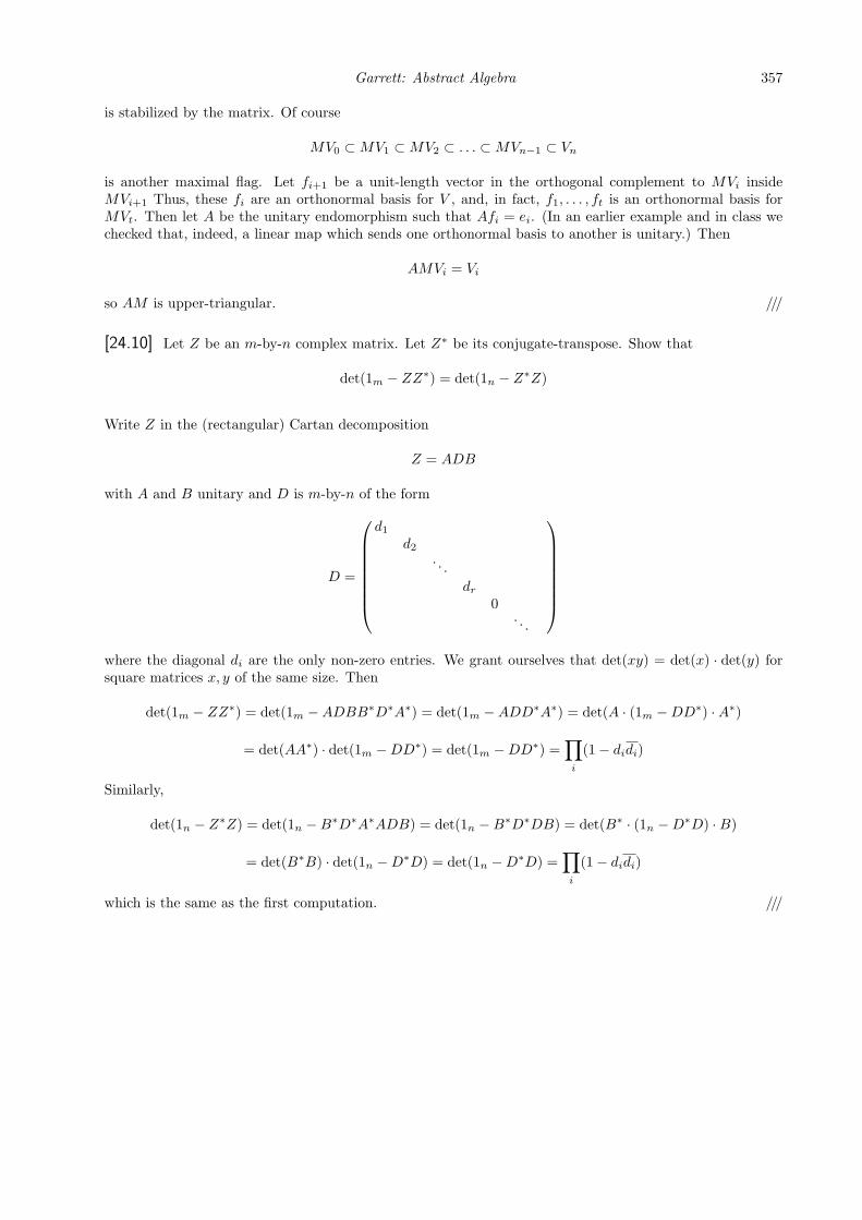
[24.10] Let Z be an m-by-n complex matrix. Let Z∗ be its conjugate-transpose. Show that

det(1m − ZZ∗) = det(1n − Z∗Z)

Write Z in the (rectangular) Cartan decomposition

Z = ADB

with A and B unitary and D is m-by-n of the form

D =

d1

d2

. . .dr

0. . .

where the diagonal di are the only non-zero entries. We grant ourselves that det(xy) = det(x) · det(y) forsquare matrices x, y of the same size. Then

det(1m − ZZ∗) = det(1m −ADBB∗D∗A∗) = det(1m −ADD∗A∗) = det(A · (1m −DD∗) ·A∗)

= det(AA∗) · det(1m −DD∗) = det(1m −DD∗) =∏i

(1− didi)

Similarly,

det(1n − Z∗Z) = det(1n −B∗D∗A∗ADB) = det(1n −B∗D∗DB) = det(B∗ · (1n −D∗D) ·B)

= det(B∗B) · det(1n −D∗D) = det(1n −D∗D) =∏i

(1− didi)

which is the same as the first computation. ///


Exercises

24.[9.0.1] Let B be a bilinear form on a vector space V over a field k. Suppose that for x, y ∈ V ifB(x, y) = 0 then B(y, x) = 0. Show that B is either symmetric or alternating, that is, either B(x, y) = B(y, x)for all x, y ∈ V or B(x, y) = −B(y, x) for all x, y ∈ V .

24.[9.0.2] Let R be a commutative ring of endomorphisms of a finite-dimensional vector space V overC with a hermitian inner product 〈, 〉. Suppose that R is closed under taking adjoints with respect to 〈, 〉.Suppose that the only R-stable subspaces of V are {0} and V itself. Prove that V is one-dimensional.

24.[9.0.3] Let T be a self-adjoint operator on a complex vector space V with hermitian inner product ,̄〉.Let W be a T -stable subspace of V . Show that the restriction of T to W is self-adjoint.

24.[9.0.4] Let T be a diagonalizable k-linear endomorphism of a k-vectorspace V . Let W be a T -stablesubspace of V . Show that T is diagonalizable on W .

24.[9.0.5] Let V be a finite-dimensional vector space over an algebraically closed field k. Let T be ak-linear endomorphism of V . Show that T can be written uniquely as T = D+N where D is diagonalizable,N is nilpotent, and DN = ND.

24.[9.0.6] Let S, T be commuting k-linear endomorphisms of a finite-dimensional vector space V over analgebraically closed field k. Show that S, T have a common non-zero eigenvector.

24. Eigenvectors, spectral theorems

Documents

Transcript of 24. Eigenvectors, spectral theorems