236875 Visual Recognition Tutorial1 Bayesian decision making with discrete probabilities – an...
33
236875 Visual Recognition Tutorial 1 Bayesian decision making with discrete probabilities – an example Looking at continuous densities Bayesian decision making with continuous probabilities – an example The Bayesian Doctor Example Tutorial 2 – the outline
-
date post
20-Dec-2015 -
Category
Documents
-
view
230 -
download
0
Transcript of 236875 Visual Recognition Tutorial1 Bayesian decision making with discrete probabilities – an...

236875 Visual Recognition Tutorial 1
Bayesian decision making with discrete
probabilities – an example
Looking at continuous densities
Bayesian decision making with continuous
probabilities – an example
The Bayesian Doctor Example
Tutorial 2 – the outline
236875 Visual Recognition Tutorial 2
Prior Probability
• w - state of nature, e.g.– w1 the object is a fish, w2 the object is a bird,
etc.
– w1 the course is good, w2 the course is bad
– etc.
• A priory probability (or prior) P(wi)
236875 Visual Recognition Tutorial 3
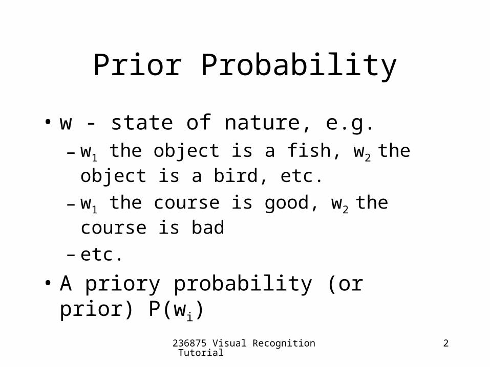
Class-Conditional Probability
• Observation x, e.g.– the objects has wings– The object’s length is 20 cm– The first lecture is interesting
• Class-conditional probability density (mass) function p(x|w)
236875 Visual Recognition Tutorial 4
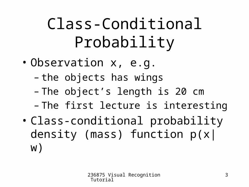
Bayes Formula
• Suppose the priors P(wj) and conditional densities p(x|wj) are known,
( | ) ( )( | )
( )j j
j
p x PP x
p x
posterior
likelihood prior
evidence
236875 Visual Recognition Tutorial 5
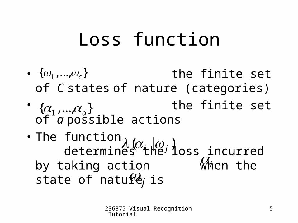
Loss function
• the finite set of C states of nature (categories)
• the finite set of a possible actions
• The function determines the loss incurred by taking action when the state of nature is
( | )i j
1{ ,..., }c
1{ ,..., }a
ij

236875 Visual Recognition Tutorial 6
Conditional Risk
• Suppose we observe a particular x and that we consider taking action
• If the true state of nature is , the incurred loss is
The expected loss,
The conditional risk:
ij
( | )i j
1
( | ) ( | ) ( | )c
i i j jj
R x P x
1
( ) ( | ) ( )c
i i j jj
R P

236875 Visual Recognition Tutorial 7
Decision Rule
• Decision rule is - what action to take in each situation
• Overall risk
• is chosen so that is minimized for each x
• Decision rule: minimize the overall risk
( ( ) | ) ( )R R x x p x dx( )x ( ( ))R x
( )x
236875 Visual Recognition Tutorial 8
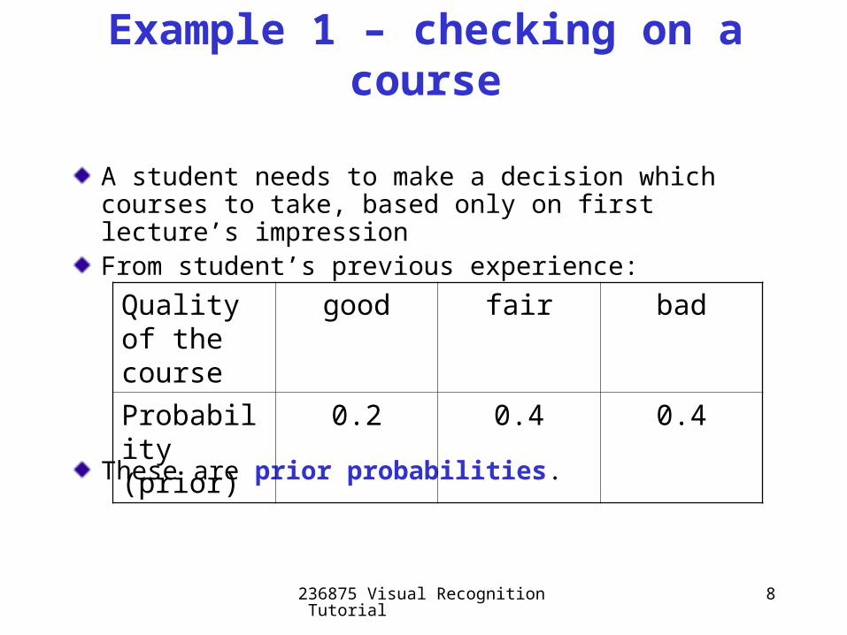
Example 1 – checking on a course
A student needs to make a decision which courses to take, based only on first lecture’s impressionFrom student’s previous experience:
These are prior probabilities.
Quality of the course
good fair bad
Probability (prior)
0.2 0.4 0.4
236875 Visual Recognition Tutorial 9
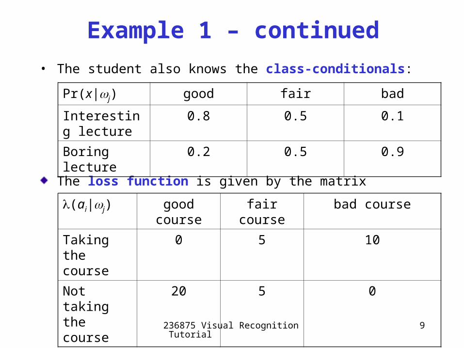
Example 1 – continued
• The student also knows the class-conditionals:
The loss function is given by the matrix
Pr(x|j) good fair bad
Interesting lecture
0.8 0.5 0.1
Boring lecture 0.2 0.5 0.9
(ai|j) good course fair course bad course
Taking the course
0 5 10
Not taking the course
20 5 0
236875 Visual Recognition Tutorial 10
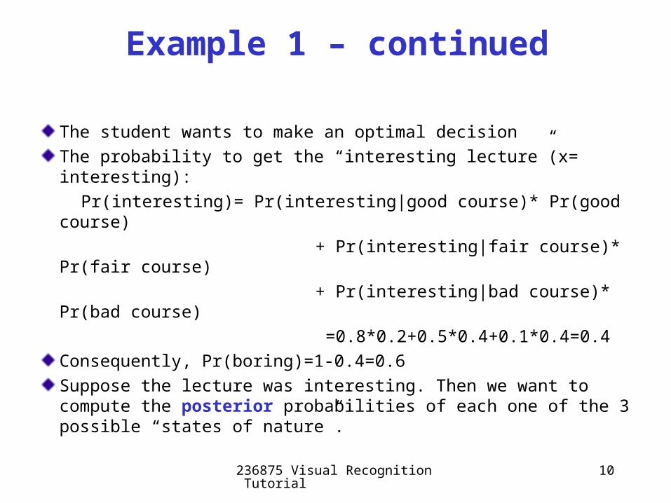
The student wants to make an optimal decision
The probability to get the “interesting lecture”(x= interesting):
Pr(interesting)= Pr(interesting|good course)* Pr(good course)
+ Pr(interesting|fair course)* Pr(fair course)
+ Pr(interesting|bad course)* Pr(bad course)
=0.8*0.2+0.5*0.4+0.1*0.4=0.4
Consequently, Pr(boring)=1-0.4=0.6
Suppose the lecture was interesting. Then we want to compute the posterior probabilities of each one of the 3 possible “states of nature”.
Example 1 – continued
236875 Visual Recognition Tutorial 11
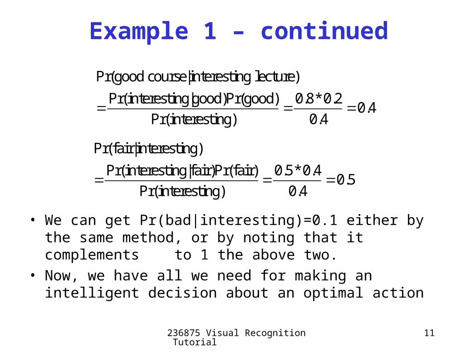
• We can get Pr(bad|interesting)=0.1 either by the same method, or by noting that it complements to 1 the above two.
• Now, we have all we need for making an intelligent decision about an optimal action
Example 1 – continued
Pr(good course|interesting lecture)
Pr(interesting|good)Pr(good) 0.8*0.20.4
Pr(interesting) 0.4
Pr(fair|interesting)
Pr(interesting|fair)Pr(fair) 0.5*0.40.5
Pr(interesting) 0.4
236875 Visual Recognition Tutorial 12
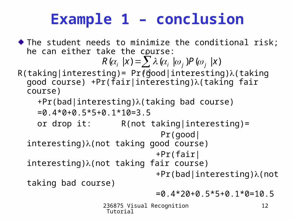
The student needs to minimize the conditional risk; he can either take the course:
R(taking|interesting)= Pr(good|interesting)(taking good course) +Pr(fair|interesting)(taking fair course)
+Pr(bad|interesting)(taking bad course) =0.4*0+0.5*5+0.1*10=3.5 or drop it: R(not taking|interesting)= Pr(good|interesting)(not taking good course) +Pr(fair|interesting)(not taking fair course) +Pr(bad|interesting)(not taking bad course) =0.4*20+0.5*5+0.1*0=10.5
Example 1 – conclusion
1
( | ) ( | ) ( | )c
i i j jj
R x P x

236875 Visual Recognition Tutorial 13
So, if the first lecture was interesting, the student will minimize the conditional risk by taking the course.
In order to construct the full decision function, we need to define the risk minimization action for the case of boring lecture, as well.
Constructing an optimal decision function
236875 Visual Recognition Tutorial 14
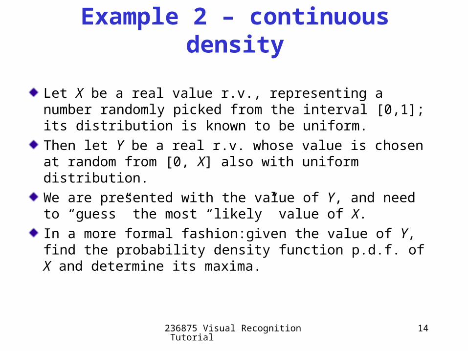
Let X be a real value r.v., representing a number randomly picked from the interval [0,1]; its distribution is known to be uniform.
Then let Y be a real r.v. whose value is chosen at random from [0, X] also with uniform distribution.
We are presented with the value of Y, and need to “guess” the most “likely” value of X.
In a more formal fashion:given the value of Y, find the probability density function p.d.f. of X and determine its maxima.
Example 2 – continuous density
236875 Visual Recognition Tutorial 15
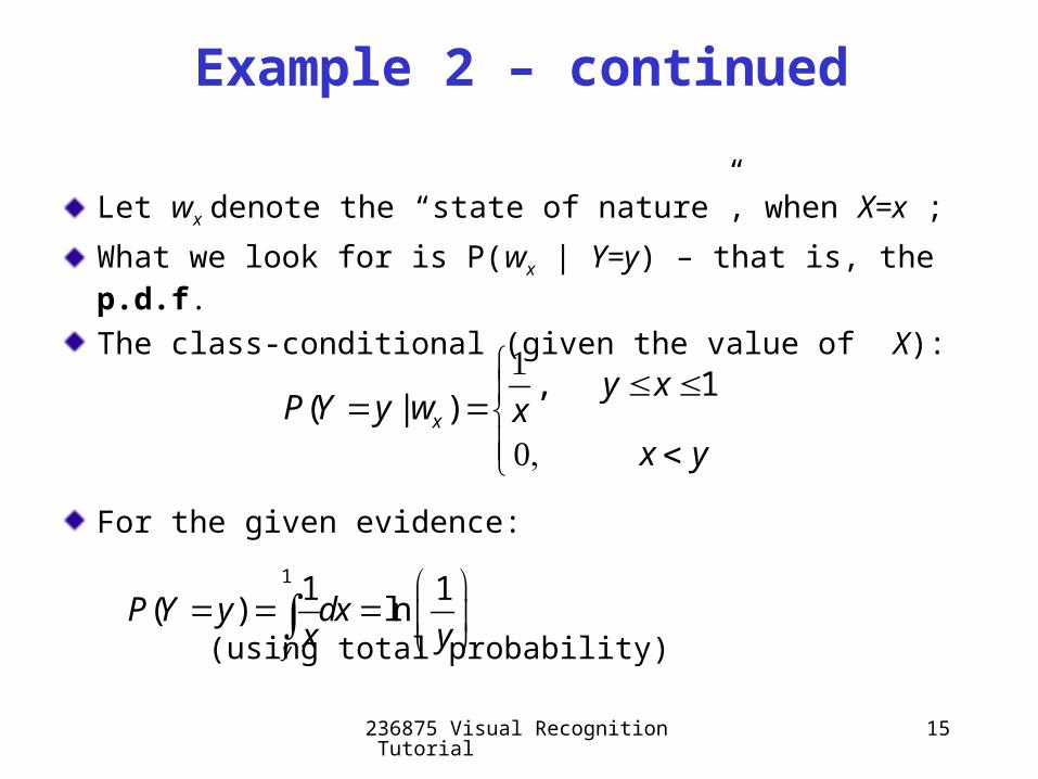
Let wx denote the “state of nature”, when X=x ;
What we look for is P(wx | Y=y) – that is, the p.d.f.
The class-conditional (given the value of X):
For the given evidence:
(using total probability)
Example 2 – continued
, 1( | )x
y xP Y y w x
x y
1 1 1( ) ln
y
P Y y dxx y
236875 Visual Recognition Tutorial 16
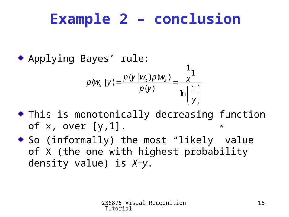
Applying Bayes’ rule:
This is monotonically decreasing function of x, over [y,1].
So (informally) the most “likely” value of X (the one with highest probability density value) is X=y.
Example 2 – conclusion
11( | ) ( )
( | )( ) 1
ln
x xx
p y w p w xp w yp y
y

236875 Visual Recognition Tutorial 17
Illustration – conditional p.d.f.
0 0.1 0.2 0.3 0.4 0.5 0.6 0.7 0.8 0.9 10
0.5
1
1.5
2
2.5
3
3.5The conditional density p(x|y=0.6)
236875 Visual Recognition Tutorial 18
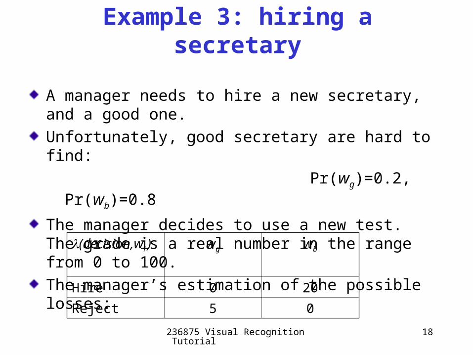
A manager needs to hire a new secretary, and a good one.
Unfortunately, good secretary are hard to find:
Pr(wg)=0.2, Pr(wb)=0.8
The manager decides to use a new test. The grade is a real number in the range from 0 to 100.
The manager’s estimation of the possible losses:
Example 3: hiring a secretary
(decision,wi ) wg wb
Hire 0 20
Reject 5 0
236875 Visual Recognition Tutorial 19
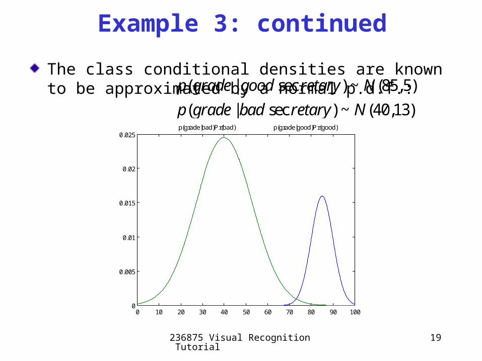
The class conditional densities are known to be approximated by a normal p.d.f.:
Example 3: continued
( | sec ) ~ (85,5)
( | sec ) ~ (40,13)
p grade good retary N
p grade bad retary N
0 10 20 30 40 50 60 70 80 90 1000
0.005
0.01
0.015
0.02
0.025 p(grade|bad)Pr(bad) p(grade|good)Pr(good)
236875 Visual Recognition Tutorial 20
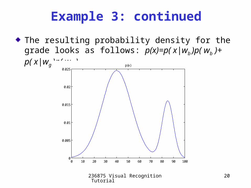
The resulting probability density for the grade looks as follows: p(x)=p( x|wb )p( wb )+ p( x|wg )p( wg )
Example 3: continued
0 10 20 30 40 50 60 70 80 90 1000
0.005
0.01
0.015
0.02
0.025p(x)
236875 Visual Recognition Tutorial 21
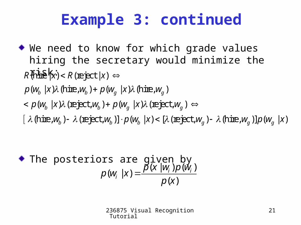
We need to know for which grade values hiring the secretary would minimize the risk:
The posteriors are given by
Example 3: continued
(hire | ) (reject | )
( | ) (hire, ) ( | ) (hire, )
( | ) (reject, ) ( | ) (reject, )
(hire, ) (reject, )] ( | ) [ (reject, ) (hire, )] ( | )
b b g g
b b g g
b b b g g g
R x R x
p w x w p w x w
p w x w p w x w
w w p w x w w p w x
( | ) ( )( | )
( )i i
i
p x w p wp w x
p x
236875 Visual Recognition Tutorial 22
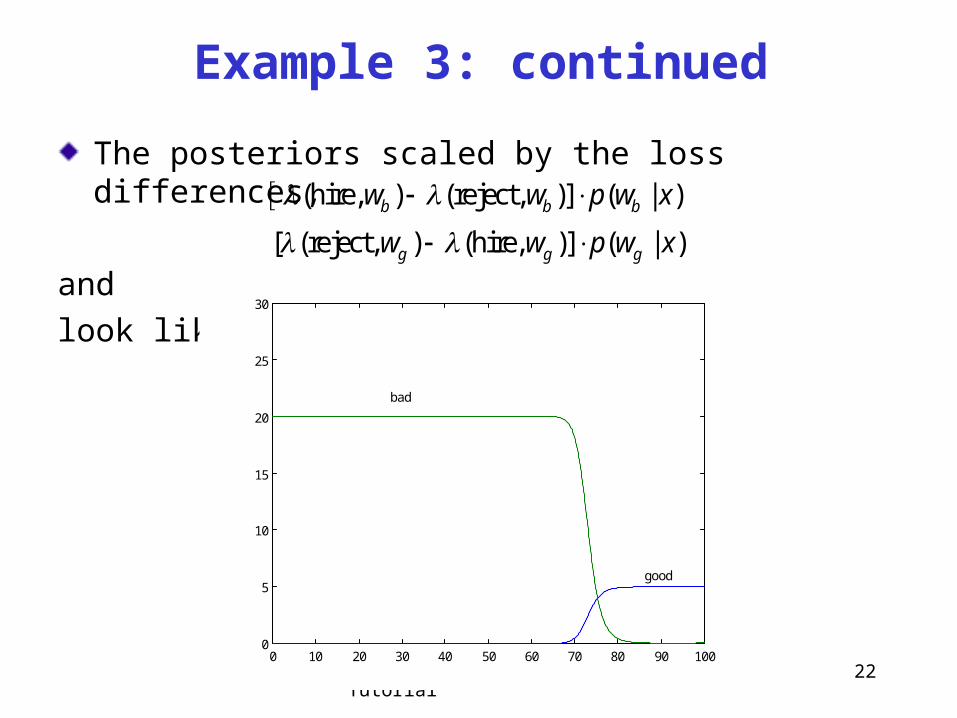
The posteriors scaled by the loss differences,
and
look like:
Example 3: continued
(hire, ) (reject, )] ( | )b b bw w p w x
[ (reject, ) (hire, )] ( | )g g gw w p w x
0 10 20 30 40 50 60 70 80 90 1000
5
10
15
20
25
30
bad
good
236875 Visual Recognition Tutorial 23
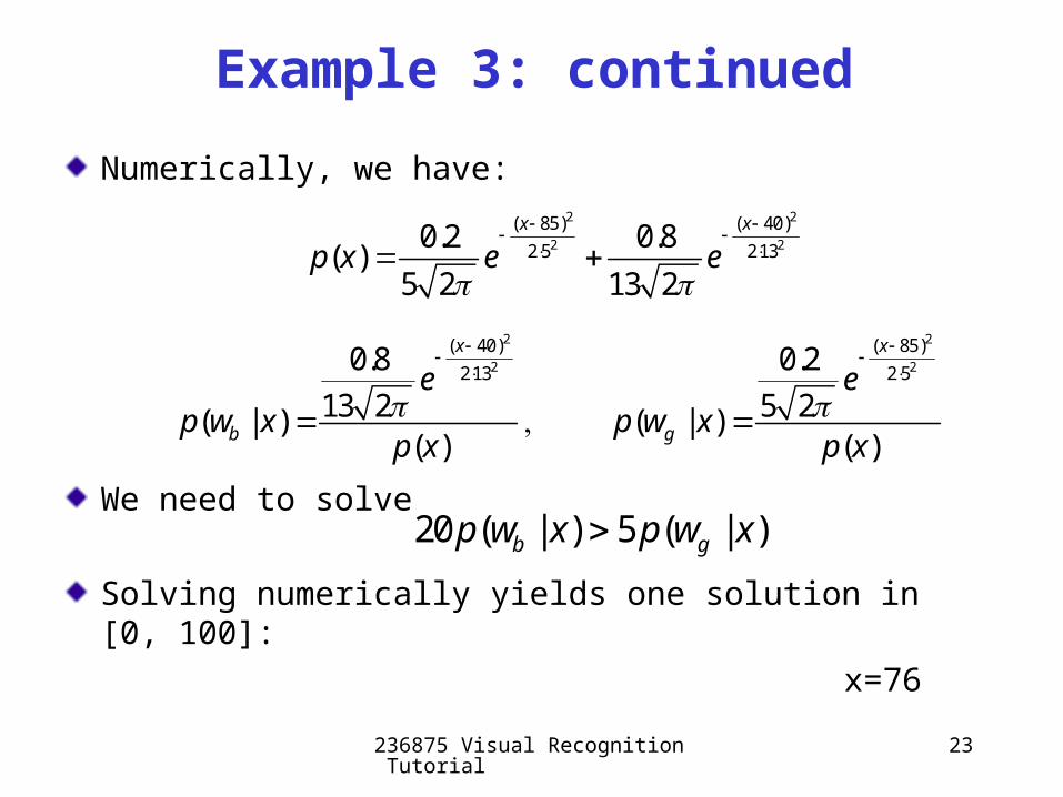
Numerically, we have:
We need to solve
Solving numerically yields one solution in [0, 100]:
x=76
Example 3: continued
2 2
2 2
( 85) ( 40)
2 5 2 130.2 0.8( )
5 2 13 2
x x
p x e e
2 2
2 2
( 40) ( 85)
2 13 2 50.8 0.2
13 2 5 2( | ) ( | )( ) ( )
x x
b g
e ep w x p w x
p x p x
20 ( | ) 5 ( | )b gp w x p w x
236875 Visual Recognition Tutorial 24
The Bayesian Doctor ExampleA person doesn’t feel well and goes to the doctor.Assume two states of nature:
1 : The person has a common flue.
2 : The person is really sick (a vicious bacterial infection). The doctors prior is:
This doctor has two possible actions: ``prescribe’’ hot tea or antibiotics. Doctor can use prior and predict optimally: always flue. Therefore doctor will always prescribe hot tea.
1.0)( 2 p9.0)( 1 p

236875 Visual Recognition Tutorial 25
• But there is very high risk: Although this doctor can diagnose with very high rate of success using the prior, (s)he can lose a patient once in a while.
• Denote the two possible actions:
a1 = prescribe hot tea
a2 = prescribe antibiotics
• Now assume the following cost (loss) matrix:
01
100
2
1
21
,
a
aji
The Bayesian Doctor - Cntd.
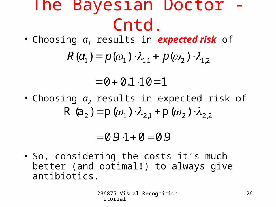
236875 Visual Recognition Tutorial 26
• Choosing a1 results in expected risk of
• Choosing a2 results in expected risk of
• So, considering the costs it’s much better (and optimal!) to always give antibiotics.
1101.00
)()()( 2,121,111
ppaR
9.0019.0
)()()( 2,221,212
ppaR
The Bayesian Doctor - Cntd.
236875 Visual Recognition Tutorial 27
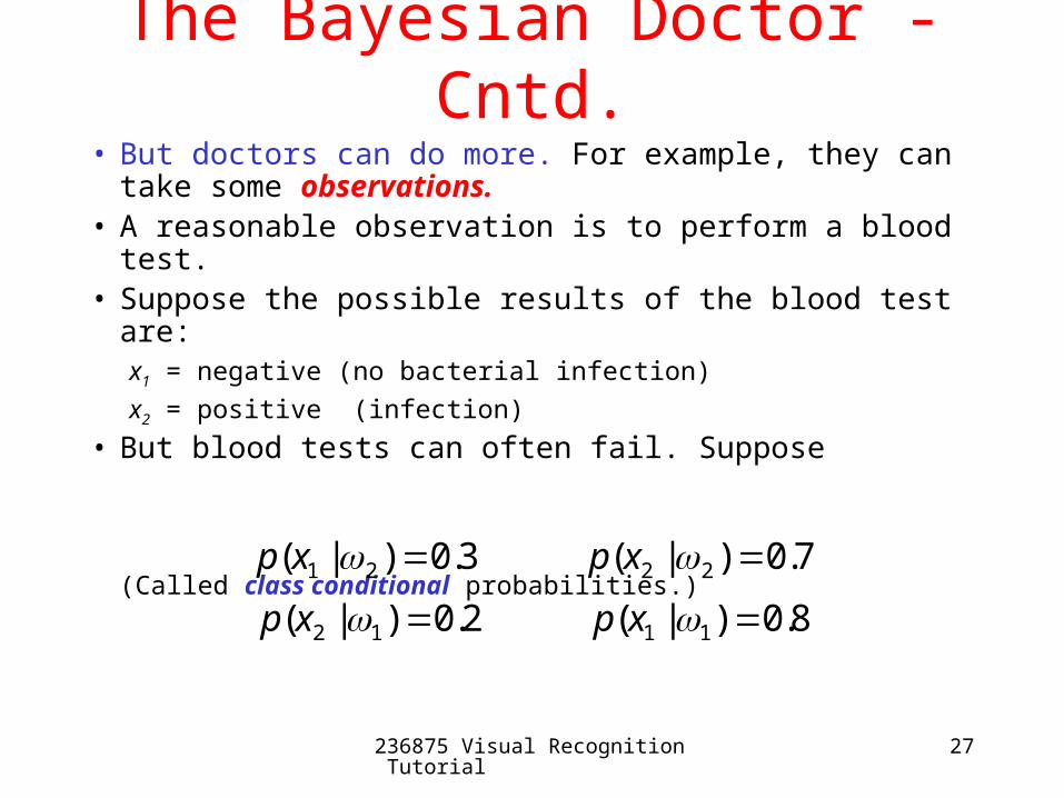
• But doctors can do more. For example, they can take some observations.
• A reasonable observation is to perform a blood test.• Suppose the possible results of the blood test are:
x1 = negative (no bacterial infection)
x2 = positive (infection)
• But blood tests can often fail. Suppose
(Called class conditional probabilities.)7.0)|(3.0)|( 2221 xpxp
8.0)|(2.0)|( 1112 xpxp
The Bayesian Doctor - Cntd.
236875 Visual Recognition Tutorial 28
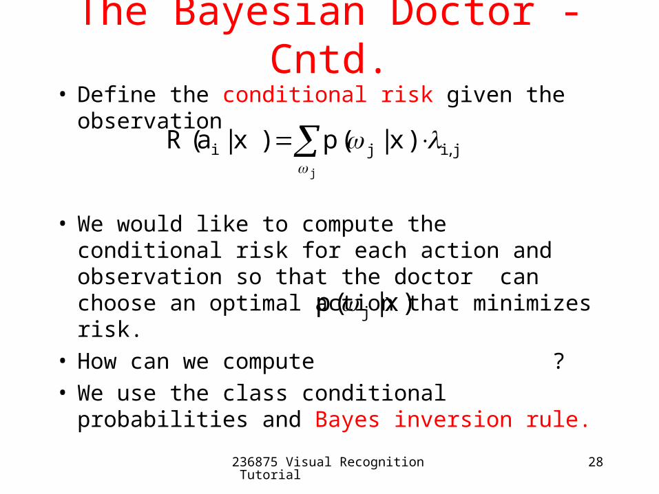
• Define the conditional risk given the observation
• We would like to compute the conditional risk for each action and observation so that the doctor can choose an optimal action that minimizes risk.
• How can we compute ? • We use the class conditional probabilities and
Bayes inversion rule.
jiji xpxaRj
,)|()|(
)|( xp j
The Bayesian Doctor - Cntd.
236875 Visual Recognition Tutorial 29
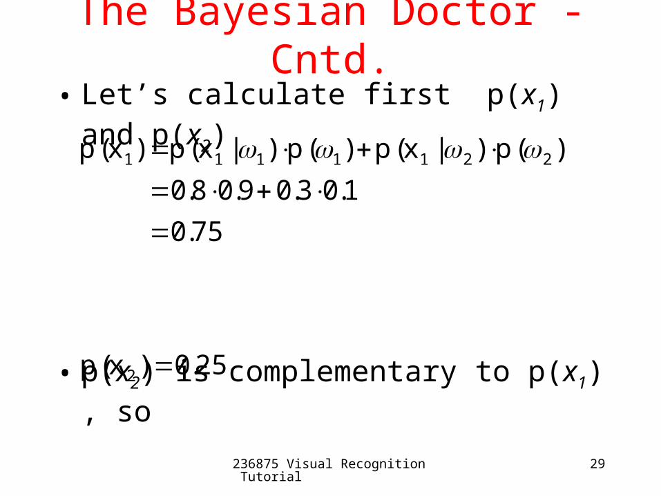
• Let’s calculate first p(x1) and p(x2)
• p(x2) is complementary to p(x1) , so
75.0
1.03.09.08.0
)()|()()|()( 2211111
pxppxpxp
25.0)( 2 xp
The Bayesian Doctor - Cntd.
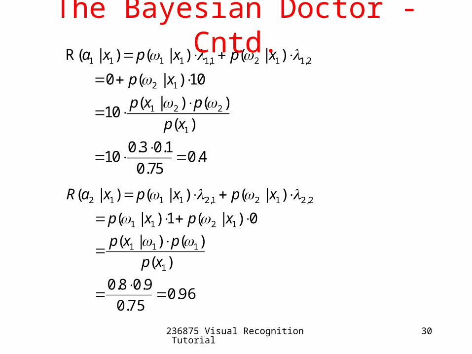
236875 Visual Recognition Tutorial 30
1 1 1 1 1,1 2 1 1,2
2 1
1 2 2
1
R( | ) ( | ) ( | )
0 ( | ) 10
( | ) ( )10
( )
0.3 0.110 0.4
0.75
a x p x p x
p x
p x p
p x
96.075.0
9.08.0
)(
)()|(
0)|(1)|(
)|()|()|(
1
111
1211
2,2121,21112
xp
pxp
xpxp
xpxpxaR
The Bayesian Doctor - Cntd.

236875 Visual Recognition Tutorial 31
8.225.0
1.07.010
)(
)()|(10
10)|(0
)|()|()|(
2
222
22
2,1221,12121
xp
pxp
xp
xpxpxaR
72.025.0
9.02.0
)(
)()|(
0)|(1)|(
)|()|()|(
2
112
2221
2,2221,22122
xppxp
xpxp
xpxpxaR
The Bayesian Doctor - Cntd.

236875 Visual Recognition Tutorial 32
• To summarize:
• Whenever we encounter an observation x, we can minimize the expected loss by minimizing the conditional risk.
• Makes sense: Doctor chooses hot tea if blood test is negative, and antibiotics otherwise.
4.0)|( 11 xaR96.0)|( 12 xaR8.2)|( 21 xaR72.0)|( 22 xaR
The Bayesian Doctor - Cntd.
236875 Visual Recognition Tutorial 33
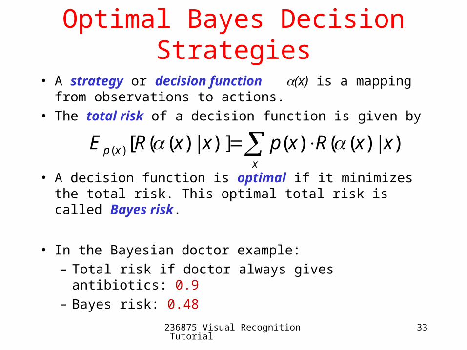
Optimal Bayes Decision Strategies
• A strategy or decision function (x) is a mapping from observations to actions.
• The total risk of a decision function is given by
• A decision function is optimal if it minimizes the total risk. This optimal total risk is called Bayes risk.
• In the Bayesian doctor example:
– Total risk if doctor always gives antibiotics: 0.9
– Bayes risk: 0.48
x
xp xxRxpxxRE )|)(()()]|)(([)(