230B: Public Economics Labor Supply Responses to …saez/course/Labortaxes/laborsupply/labor...230B:...

230B: Public Economics

Labor Supply Responses to Taxes and

Transfers

Emmanuel Saez

Berkeley

1

MOTIVATION

1) Labor supply responses to taxation are of fundamental im-portance for income tax policy [efficiency costs and optimaltax formulas]

2) Labor supply responses along many dimensions:

(a) Intensive: hours of work on the job, intensity of work,occupational choice [including education]

(b) Extensive: whether to work or not [e.g., retirement andmigration decisions]

3) Reported earnings for tax purposes can also vary due to (a)tax avoidance [legal tax minimization], (b) tax evasion [illegalunder-reporting]

4) Different responses in short-run and long-run: long-run re-sponse most important for policy but hardest to estimate

2

STATIC MODEL: SETUP

Baseline model: (a) static, (b) linearized tax system, (c) pureintensive margin choice, (d) single hours choice, (e) no fric-tions

Let c denote consumption and l hours worked, utility u(c, l)increases in c, and decreases in l

Individual earns wage w per hour (net of taxes) and has y innon-labor income

Key example: pre-tax wage rate wp and linear tax system withtax rate τ and demogrant G ⇒ c = wp(1− τ)l +G

Individual solves

maxc,l

u(c, l) subject to c = wl + y

3

LABOR SUPPLY BEHAVIOR

FOC: wuc+ul = 0 defines uncompensated (Marshallian) labor

supply function lu(w, y)

Uncompensated elasticity of labor supply: εu = (w/l)∂lu/∂w

[% change in hours when net wage w ↑ by 1%]

Income effect parameter: η = w∂l/∂y ≤ 0: $ increase in earn-

ings if person receives $1 extra in non-labor income

Compensated (Hicksian) labor supply function lc(w, u) which

minimizes cost wl− c st to constraint u(c, l) ≥ u.

Compensated elasticity of labor supply: εc = (w/l)∂lc/∂w > 0

Slutsky equation: ∂l/∂w = ∂lc/∂w + l∂l/∂y ⇒ εu = εc + η

4

0 labor supply 𝑙

R

𝑐 =

consumption

slope= 𝑤

Marshallian Labor Supply

𝑙(𝑤, 𝑅)

𝑙 ∗

𝑐 = 𝑤𝑙 + 𝑅

Indifference

Curve

Labor Supply Theory

0 labor supply 𝑙

𝑐 =

consumption

slope= 𝑤

Hicksian Labor Supply

𝑙𝑐(𝑤, 𝑢)

Labor Supply Theory

utility 𝑢

0 labor supply 𝑙

𝑐 Labor Supply Income Effect

R

R+∆R

𝑙(𝑤, 𝑅) 𝑙(𝑤, 𝑅+∆R)

𝜂 = 𝑤𝜕𝑙

𝜕𝑅≤ 0

0 labor supply 𝑙

𝑐 Labor Supply Substitution Effect

slope= 𝑤

utility 𝑢

slope= 𝑤 + ∆𝑤

𝑙𝑐(𝑤 + ∆𝑤, 𝑢) 𝑙𝑐(𝑤, 𝑢)

𝜀𝑐 =𝑤

𝑙

𝜕𝑙𝑐

𝜕𝑤> 0

0 labor supply 𝑙

𝑐 Uncompensated Labor Supply Effect

slope= 𝑤

slope= 𝑤 + ∆𝑤

𝑙(𝑤 + ∆𝑤, 𝑅)

𝑙(𝑤, 𝑅)

substitution effect: 𝜀𝑐 > 0

income effect

𝜂 ≤ 0

𝜀𝑢 = 𝜀𝑐 + 𝜂

BASIC CROSS SECTION ESTIMATION

Data on hours or work, wage rates, non-labor income startedbecoming available in the 1960s when first micro surveys andcomputers appeared:

Simple OLS regression:

li = α+ βwi + γyi +Xiδ + εi

wi is the net-of-tax wage rate

yi measures non-labor income [including spousal earnings forcouples]

Xi are demographic controls [age, experience, education, etc.]

β measures uncompensated wage effects, and γ income effects[can be converted to εu, η]

6

BASIC CROSS SECTION RESULTS

1. Male workers [primary earners when married] (Pencavel,

1986 survey):

a) Small effects εu = 0, η = −0.1, εc = 0.1 with some variation

across estimates (sometimes εc < 0).

2. Female workers [secondary earners when married] (Killingsworth

and Heckman, 1986):

Much larger elasticities on average, with larger variations across

studies. Elasticities go from zero to over one. Average around

0.5. Significant income effects as well

Female labor supply elasticities have declined overtime as women

become more attached to labor market (Blau-Kahn JOLE’07)

7

KEY ISSUE: w correlated with tastes for work

li = α+ βwi + γyi + εi

Identification is based on cross-sectional variation in wi: com-paring hours of work of highly skilled individuals (high wi) tohours of work of low skilled individuals (low wi)

If highly skilled workers have more taste for work (independentof the wage effect), then εi is positively correlated with wileading to an upward bias in OLS

Plausible scenario: hard workers acquire better education andhence have higher wages

Controlling for Xi can help but can never be sure that we havecontrolled for all the factors correlated with wi and tastes forwork: Omitted variable bias

⇒ Tax changes provide more compelling identification

8

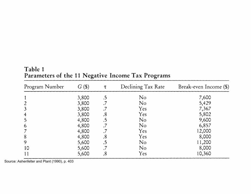
Negative Income Tax (NIT) Experiments

1) Best way to resolve identification problems: exogenouslychange taxes/transfers with a randomized experiment

2) NIT experiment conducted in 1960s/70s in Denver, Seattle,and other cities

3) First major social experiment in U.S. designed to test pro-posed transfer policy reform

4) Provided lump-sum welfare grants G combined with a steepphaseout rate τ (50%-80%) [based on family earnings]

5) Analysis by Rees (1974), Munnell (1986) book, Ashenfelterand Plant JOLE’90, and others

6) Several groups, with randomization within each; approx. N= 75 households in each group

9

Raj Chetty () Labor Supply Harvard, Fall 2009 87 / 156

Source: Ashenfelter and Plant (1990), p. 403

NIT Experiments: Findings

See Ashenfelter and Plant JHR’ 90 for non-parametric evi-dence. More parametric evidence in earlier work. Key results:

1) Significant labor supply response but small overall

2) Implied earnings elasticity for males around 0.1

3) Implied earnings elasticity for women around 0.5

4) Academic literature not careful to decompose responsealong intensive and extensive margin

5) Response of women is concentrated along the extensivemargin (can only be seen in official govt. report)

6) Earnings of treated women who were working before theexperiment did not change much

11

From true experiment to “natural experiments”

True experiments are costly to implement and hence rare

However, real economic world (nature) provides variation thatcan be exploited to estimate behavioral responses ⇒ “NaturalExperiments”

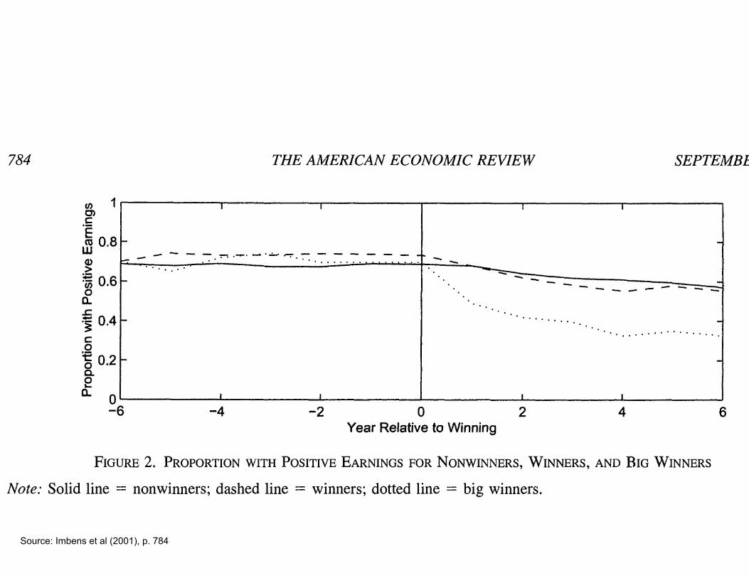
Natural experiments sometimes come very close to true ex-periments: Imbens, Rubin, Sacerdote AER ’01 did a survey oflottery winners and non-winners matched to Social Securityadministrative data to estimate income effects

Lottery generates random assignment conditional on playing

Find significant but relatively small income effects: η = w∂l/∂y

between -0.05 and -0.10

Identification threat: differential response-rate among groups

12

784 THE AMERICAN ECONOMIC REVIEW SEPTEMBER 2001

co 0.8-

0.6 -

0~ *'0.4 ..

0

-6 -4 -2 0 2 4 6 Year Relative to Winning

FIGURE 2. PROPORTION WITH POSITIVE EARNINGS FOR NONWINNERS, WINNERS, AND BIG WINNERS

Note: Solid line = nonwinners; dashed line = winners; dotted line = big winners.

type accounts, including IRA's, 401(k) plans, and other retirement-related savings. The second consists of stocks, bonds, and mutual funds and general savings.13 We construct an additional variable "total financial wealth," adding up the two savings categories.14 Wealth in the various savings accounts is somewhat higher than net wealth in housing, $133,000 versus $122,000. The distributions of these financial wealth variables are very skewed with, for example, wealth in mutual funds for the 414 respondents ranging from zero to $1.75 million, with a mean of $53,000, a median of $10,000, and 35 percent zeros.

The critical assumption underlying our analysis is that the magnitude of the lottery prize is random. Given this assumption the background characteristics and pre-lottery earnings should not differ significantly between nonwinners and winners. However, the t-statistics in Table 1 show that nonwinners are significantly more educated than winners, and they are also older.

This likely reflects the differences between sea- son ticket holders and single ticket buyers as the differences between all winners and the big winners tend to be smaller.15 To investigate further whether the assumption of random assignment of lottery prizes is more plausible within the more narrowly defined subsamples, we regressed the lottery prize on a set of 21 pre-lottery variables (years of education, age, number of tickets bought, year of winning, earnings in six years prior to winning, dummies for sex, college, age over 55, age over 65, for working at the time of winning, and dummies for positive earnings in six years prior to winning). Testing for the joint significance of all 21 covariates in the full sample of 496 observations led to a chi-squared statistic of 99.9 (dof 21), highly significant (p < 0.001). In the sample of 237 winners, the chi-squared statistic was 64.5, again highly significant (p < 0.001). In the sample of 193 small winners, the chi-squared statistic was 28.6, not significant at the 10- percent level. This provides some support for assumption of random assignment of the lottery prizes, at least within the subsample of small winners. 13 See the Appendix in Imbens et al. (1999) for the

questionnaire with the exact formulation of the questions. 14 To reduce the effect of item nonresponse for this last

variable, total financial wealth, we added zeros to all miss- ing savings categories for those people who reported positive savings for at least one of the categories. That is, if someone reports positive savings in the category "retirement accounts," but did not answer the question for mutual funds, we impute a zero for mutual funds in the construction of total financial wealth. For the 462 observations on total financial wealth, zeros were imputed for 27 individuals for retirement savings and for 30 individuals for mutual funds and general savings. As a result, the average of the two savings categories does not add up to the average of total savings, and the number of observations for the total savings variable is larger than that for each of the two savings categories.

15 Although the differences between small and big winners are smaller than those between winners and losers, some of them are still significant. The most likely cause is the differential nonresponse by lottery prize. Because we do know for all individuals, respondents or nonrespondents, the magnitude of the prize, we can directly investigate the correlation between response and prize. Such a non-zero correlation is a necessary condition for nonresponse to lead to bias. The t-statistic for the slope coefficient in a logistic regression of response on the logarithm of the yearly prize is -3.5 (the response rate goes down with the prize), lending credence to this argument.

Source: Imbens et al (2001), p. 784

VOL. 91 NO. 4 IMBENS ET AL.: EFFECTS OF UNEARNED INCOME 783

m 0 , " .........

10-

O

-6 -4 -2 0 2 4 6 Year Relative to Winning

FIGURE 1. AVERAGE EARNINGS FOR NONWINNERS, WINNERS, AND BIG WINNERS

Note: Solid line = nonwinners; dashed line = winners; dotted line = big winners.

On average the individuals in our basic sample won yearly prizes of $26,000 (averaged over the $55,000 for winners and zero for nonwinners). Typically they won 10 years prior to completing our survey in 1996, implying they are on average halfway through their 20 years of lottery payments when they responded in 1996. We asked all individuals how many tickets they bought in a typical week in the year they won the lottery.!1 As ex- pected, the number of tickets bought is consider- ably higher for winners than for nonwinners. On average, the individuals in our basic sample are 50 years old at the time of winning, which, for the average person was in 1986; 35 percent of the sample was over 55 and 15 percent was over 65 years old at the time of winning; 63 percent of the sample was male. The average number of years of schooling, calculated as years of high school plus years of college plus 8, is equal to 13.7; 64 percent claimed at least one year of college.

We observe, for each individual in the basic sample, Social Security earnings for six years pre- ceding the time of winning the lottery, for the year they won (year zero), and for six years following winning. Average earnings, in terms of 1986 dollars, rise over the pre-winning period from $13,930 to $16,330, and then decline back to $13,290 over the post-winning period. For those with positive Social Security earnings, average earnings rise over the entire 13-year period from $20,180 to $24,300. Participation rates, as mea- sured by positive Social Security earnings, grad-

ually decline over the 13 years, starting at around 70 percent before going down to 56 percent. Fig- ures 1 and 2 present graphs for average earnings and the proportion of individuals with positive earnings for the three groups, nonwinners, winners, and big winners. One can see a modest decline in earnings and proportion of individuals with positive earnings for the full winner sample compared to the nonwinners after winning the lottery, and a sharp and much larger decline for big winners at the time of winning. A simple difference-in-differences type estimate of the marginal propensity to earn out of unearned income (mpe) can be based on the ratio of the difference in the average change in earnings before and after winning the lottery for two groups and the difference in the average prize for the same two groups. For the winners, the difference in average earnings over the six post-lottery years and the six pre- lottery years is -$1,877 and for the nonwinners the average change is $448. Given a difference in average prize of $55,000 for the winner/nonwinners comparison, the estimated mpe is (- 1,877 - 448)/(55,000 - 0) = -0.042 (SE 0.016). For the big-winners/small-winners comparison, this estimate is -0.059 (SE 0.018). In Section IV we report estimates for this quantity using more so- phisticated analyses.

On average the value of all cars was $18,200. For housing the average value was $166,300, with an average mortgage of $44,200.12 We aggregated the responses to financial wealth into two categories. The first concerns retirement

" Because there were some extremely large numbers (up to 200 tickets per week), we transformed this valiable somewhat arbitrarily by taking the minimum of the number reported and ten. The results were not sensitive to this transformation.

12 Note that this is averaged over the entire sample, with zeros included for the 7 percent of respondents who reported not owning their homes.

Source: Imbens et al. (2001), p. 783

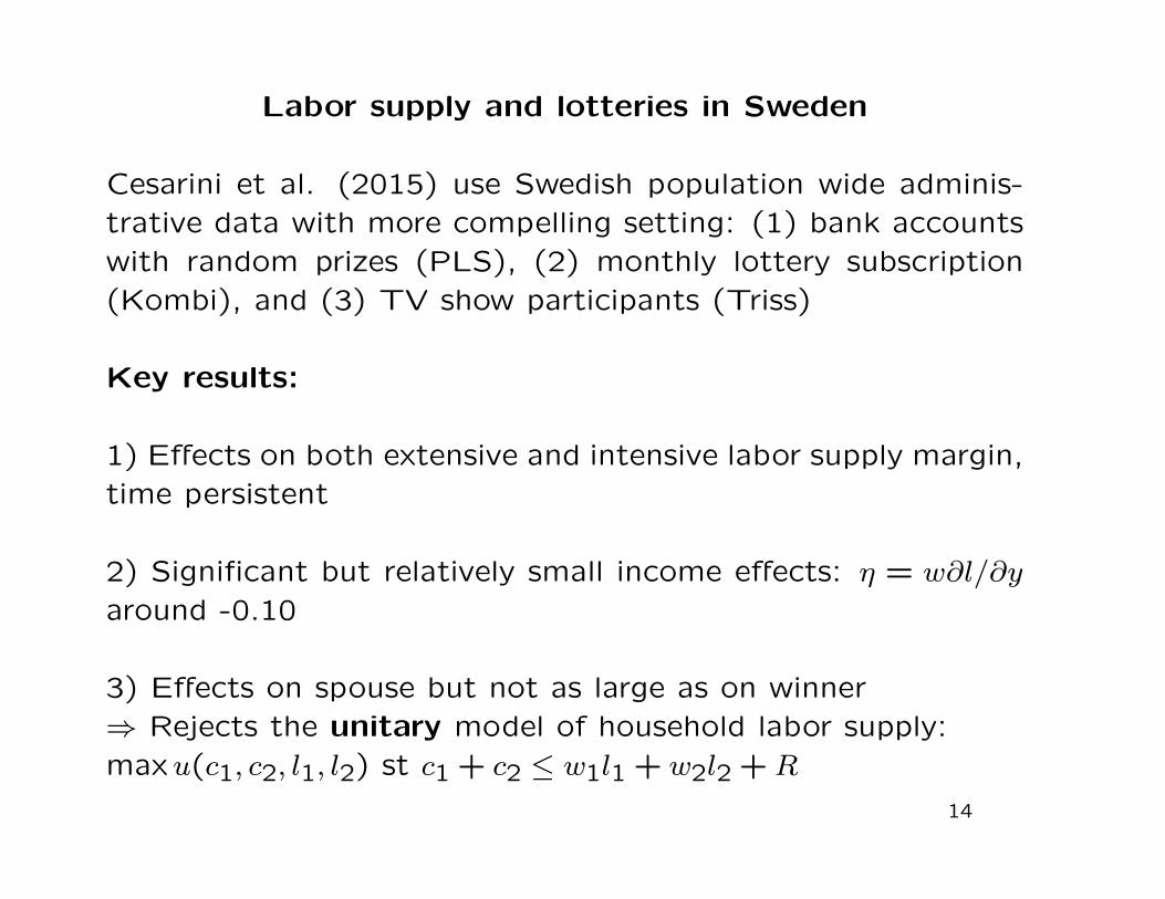
Labor supply and lotteries in Sweden

Cesarini et al. (2015) use Swedish population wide adminis-trative data with more compelling setting: (1) bank accountswith random prizes (PLS), (2) monthly lottery subscription(Kombi), and (3) TV show participants (Triss)

Key results:

1) Effects on both extensive and intensive labor supply margin,time persistent

2) Significant but relatively small income effects: η = w∂l/∂y

around -0.10

3) Effects on spouse but not as large as on winner⇒ Rejects the unitary model of household labor supply:maxu(c1, c2, l1, l2) st c1 + c2 ≤ w1l1 + w2l2 +R

14

Count Share Count Share Count Share Count Share Count Share

0 to 1K SEK 25,172 10.0% 0 0.0% 25,172 99.0% 0 0.0% 0 0.0%1K to 10K SEK 204,626 81.3% 204,626 92.0% 0 0.0% 0 0.0% 0 0.0%10K to 100K SEK 16,429 6.5% 15,520 7.0% 0 0.0% 909 27.8% 0 0.0%100K to 500K SEK 3,685 1.5% 1,654 0.7% 0 0.0% 2,031 62.1% 0 0.0%500K to 1M SEK 355 0.1% 195 0.1% 0 0.0% 160 4.9% 0 0.0%>1M SEK 1,481 0.6% 481 0.2% 263 1.0% 168 5.1% 569 100.0%TOTAL 251,748 222,476 25,435 3,268 569

Notes: This table reports the distribution of lottery prizes for the pooled sample and the four lottery subsamples.

Table 1. Distribution of Prizes

Pooled SampleIndividual Lottery Samples

PLS Kombi Triss-Lumpsum Triss-Monthly

t = 1 t = 23-year total

5-year total

10-year total

Event study estimate t = 1-5

(1) (2) (3) (4) (5) (6)Prize Amount (SEK/100) -1.152 -1.177 -3.219 -4.681 -8.033 -1.068

SE (0.153) (0.191) (0.517) (0.917) (1.961) (0.149)p [<0.001] [<0.001] [<0.001] [<0.001] [<0.001] [<0.001]

N 199,168 211,555 193,312 186,819 173,129 249,278

Table 2. Effect of Wealth on Individual Gross Labor Earnings

Notes: This table reports results of estimating equation (2) in the pooled lottery sample with gross labor earnings as the dependent variable. The prize amount is scaled so that a coefficient of 1.00 implies a 1 SEK increase in earningsper 100 SEK won.

Cesarini, Lindqvist, Notowidigdo, Östling NBER WP 2015

Figure 1: Effect of Wealth on Individual Gross Labor Earnings

Notes: This figure reports estimates obtained from equation (2) estimated in the pooled lottery sample with gross labor earnings as the dependent variable. A coefficient of 1.00 corresponds to an increase in annual labor earnings of 1 SEK for each 100 SEK won. Each year corresponds to a separate regression and the dashed lines show 95% confidence intervals.

-2-1

.5-1

-.50

.5C

oeffi

cien

t on

Lotte

ry W

ealth

(Sca

led

in 1

00 S

EK

)

-5 0 5 10Years Relative to Winning


Figure 4: Comparing Model-Based Estimates to Empirical Results

Notes: This figure compares the estimates obtained from equation (2) estimated in the pooled lottery sample with after-tax earnings as the dependent variable to the model-based estimates using the best-fit parameters reported in Table 5. Year 0 correspond to the year the lottery prize is awarded, and in the simulation, the prize is assumed to be awarded at end of the year, so dy/dL for that year is 0 by assumption.

Figure 5: Effect of Wealth on Gross Labor Earnings of Winners and Spouses

Notes: This figure reports estimates obtained from equation (2) estimated separately for winners, their spouses, and the household. The dependent variable is gross labor earnings. Each year corresponds to a separate regression.

-1-.8

-.6-.4

-.20

Effe

ct o

f Lot

tery

on

Labo

r Ear

ning

s

0 1 2 3 4 5 6 7 8 9 10Year Relative to Winning

Pooled Sample Estimates Model-based Simulation

-2-1

.5-1

-.50

.5In

com

e pe

r 100

SE

K W

on

0 2 4 6 8 10Years Relative to Winning

Winner's Estimates Spouse's EstimatesHousehold's Estimates


Married Women Elasticities: Blau and Kahn ’07

1) Identify elasticities from 1980-2000 using grouping instru-ment

a) Define cells (year×age×education) and compute mean wages

b) Instrument for actual wage with mean wage in cell

2) Identify purely from group-level variation, which is less con-taminated by individual endogenous choice

3) Results: (a) total hours elasticity for married women (in-cluding intensive + extensive margin) shrank from 0.4 in 1980to 0.2 in early 2000s, (b) effect of husband earnings ↓ overtime

4) Interpretation: elasticities shrink as women become moreattached to the labor force

17

Summary of Static Labor Supply Literature (SKIP)

1) Small elasticities for prime-age males

Probably institutional restrictions, need for at least one in-

come, etc. prevent a short-run response

2) Larger responses for workers who are less attached to labor

force: Married women, low income earners, retirees

3) Responses driven primarily by extensive margin

a) Extensive margin (participation) elasticity around 0.2-0.5

b) Intensive margin (hours) elasticity smaller

18

Responses to Low-Income Transfer Programs

1) Particular interest in treatment of low incomes in a pro-

gressive tax system: are they responsive to incentives?

2) Complicated set of transfer programs in US

a) In-kind: food stamps, Medicaid, public housing, job train-

ing, education subsidies

b) Cash: TANF, EITC, SSI

3) See Gruber undergrad textbook for details on institutions

19

1996 US Welfare Reform

1) Largest change in welfare policy

2) Reform modified AFDC cash welfare program to providemore incentives to work (renamed TANF)

a) Requiring recipients to go to job training or work

b) Limiting the duration for which families able to receivewelfare

c) Reducing phase-out rate of benefits

3) Variation across states because Fed govt. gave block grantswith guidelines

4) EITC also expanded during this period: general shift fromwelfare to “workfare”

20

The landscape providing assistance to poor families with children has changed substantially

175

200Contractions

AFDC/TANF Cash Benefits Per CapitaFederal welfare reform

125

150

ditures

Food Stamp Expenditures Per Capita

EITC Expenditures Per Capita

100

125

Real Expend

50

75

Per C

apita

25

4

0

1980 1985 1990 1995 2000 2005

Annual Employment Rates for Women By Marital Status and Presence of Children, 1980-2009

50%

60%

70%

80%

90%

100%

1980 1985 1990 1995 2000 2005

Single with Children

Single No Children

Married with Children

Source: Bitler and Hoynes, Brookings Papers on Economic Activity, 2011.

Welfare Reform: Two Empirical Questions

1) Incentives: did welfare reform actually increase labor supply?

a) Test whether EITC expansions affect labor supply

b) Use state welfare randomized experiments implemented be-

fore reform to assess effects of switch from AFDC to TANF

2) Benefits: did removing many people from transfer system

reduce their welfare? How did consumption change?

Focus on single mothers, who were most impacted by reform

22

Earned Income Tax Credit (EITC) program

Hotz-Scholz ’04, Eissa-Hoynes ’06, Nichols-Rothstein ’15 pro-vide detailed surveys

1) EITC started small in the 1970s but was expanded in 1986-88, 1994-96, 2008-09: today, largest means-tested cash trans-fer program [$60bn in 2012, 25m families recipients]

2) Eligibility: families with kids and low earnings.

3) Refundable Tax credit: administered as annual tax refundreceived in Feb-April, year t+ 1 (for earnings in year t)

4) EITC has flat pyramid structure with phase-in (negativeMTR), plateau, (0 MTR), and phase-out (positive MTR)

5) States have added EITC components to their income taxes[in general a percentage of the Fed EITC, great source ofnatural experiments, understudied bc CPS too small]

23

EITC Amount as a Function of Earnings

Earnings ($)

0 5000 10000 15000 20000 25000 30000 35000 40000

Subsidy: 34%

Subsidy: 40%

Phase-out tax: 16%

Phase-out tax: 21%

Single, 2+ kidsMarried, 2+ kids

Single, 1 kidMarried, 1 kid

No kids

EIT

C A

mou

nt ($

)

010

0020

0030

0040

0050

00

Source: Federal Govt

60

Figure 2. Maximum credit over time, constant 2013 dollars, by number of children

0"

1000"

2000"

3000"

4000"

5000"

6000"

7000"

1975" 1980" 1985" 1990" 1995" 2000" 2005" 2010" 2015"

Maxim

um'EITC'(201

3$)'

Year'

0"children"

1"child"

2"children"

3"children"

Source: Nichols and Rothstein (2015)

Theoretical Behavioral Responses to the EITC

Extensive margin: positive effect on Labor Force Participa-tion

Intensive margin: earnings conditional on working, mixedeffects

1) Phase in: (a) Substitution effect: work more due to wagesubsidy, (b) Income effect: work less⇒ Net effect: ambiguous;probably work more

2) Plateau: Pure income effect (no change in net wage) ⇒Net effect: work less

3) Phase out: (a) Substitution effect: work less, (b) Incomeeffect: also work less ⇒ Net effect: work less

Should expect bunching at the EITC kink points

26

Eissa and Liebman 1996

1) Pioneering study of labor force participation of single moth-

ers before/after 1986-7 EITC expansion using CPS data

2) Limitation: this expansion was relatively small

3) Diff-in-Diff strategy:

a) Treatment group: single women with kids

b) Control group: single women without kids

c) Comparison periods: 1984-1986 vs. 1988-1990

27

Source: Eissa and Liebman (1996), p. 631

Diff-in-Diff (DD) Methodology:

Step 1: Simple Difference

Outcome: LFP (labor force participation)

Two groups: Treatment group (T) which faces a change [sin-gle women with kids] and control group (C) which does not[single women without kids]

Simple Difference estimate: D = LFPT − LFPC capturestreatment effect if absent the treatment, LFP equal across2 groups

Note: this assumption always holds when T and C status israndomly assigned

Test for this assumption: Compare LFP before treatmenthappened DB = LFPTB − LFP

CB

29

Diff-in-Diff (DD) Methodology:

Step 2: Diff-in-Difference (DD)

If DB 6= 0, can estimate DD:

DD = DA −DB = LFPTA − LFPCA − [LFPTB − LFP

CB ]

(A = after reform, B = before reform)

DD is unbiased if parallel trend assumption holds:

Absent the change, difference across T and C would havestayed the same before and after

OLS Regression estimation of DD:

LFPit = β0AFTER+ β1TREAT + γAFTER · TREAT + ε

γOLS = LFPTA − LFPCA − [LFPTB − LFP

CB ]

30

Diff-in-Diff (DD) Methodology

DD most convincing when groups are very similar to start with[closer to randomized experiment]

Should always test DD using data from more periods and plotthe two time series to check parallel trend assumption

Use alternative control groups [not as convincing as potentialcontrol groups are many]

In principle, can create a DDD as the difference between actualDD and DDPlacebo (DD between 2 control groups). However,DDD of limited interest in practice because

(a) if DDPlacebo 6= 0, DD test fails, hard to believe DDD re-moves bias

(b) if DDPlacebo = 0, then DD=DDD but DDD has higher s.e.

32

Diff-in-Diff (DD) Methodology

1) DD sensitive to functional form (e.g. log vs levels) when

Dbefore 6= 0.

Example: T ↑ from 40% to 50% and C ↑ from 15% to 20%: DDlevel =

[50− 40]− [20− 15] = 5 but DDlog = log[50/40]− log[20/15] = −.06

2) To obtain elasticity estimate, need to take ratio of DDoutcometo DDpolicy change to form the Wald estimate:

e =[logLFPTA − logLFPCA ]− [logLFPTB − logLFPCB ]

log(1− τTA)− log(1− τCA )]− [log(1− τTB)− log(1− τCB )]

DDpolicy change is the 1st stage, DDoutcome is the reduced

form effect, the ratio is the 2nd stage estimate

Wald estimated with 2SLS regression:

LFPit = β0AFTER+ β1TREAT + e · log(1− τ) + ε

where log(1− τ) is instrumented with interaction AFTER · TREAT

34

Eissa and Liebman 1996: Results

1) Find a small but significant DD effect: 2.4% (larger DD

effect 4% among women with low education) ⇒ Translates

into substantial participation elasticities above 0.5

2) Note the labor force participation for women with/without

children are not great comparison groups (70% LFP vs. +90%):

time series evidence is only moderately convincing

3) Subsequent studies have used bigger 1990s EITC expan-

sions and also find positive effects on labor force participation

of single women/single mothers (Meyer-Rosenbaum 2001) but

contaminated by AFDC/TANF transition

4) Conventional standard errors probably overstate precision

35

Bertrand-Duflo-Mullainathan QJE’04

Show that conventional standard errors in fixed effects regres-sions with state reform variation are too low

Randomly generated placebo state laws: half the states passlaw at random date. Ist is one if state s has law in place attime t.

Use female wages wist in CPS data and run OLS:

logwist = As +Bt + bIst + εist

b significant (at 5% level) in 65% of cases ⇒ εist are not iid

Clustering by state*year cells is not enough (significant 45%of the time)

Need to cluster at state level to obtain reasonable s.e. becauseof strong serial correlation within states

36

Bunching at Kinks (Saez AEJ-EP’10)

Key prediction of standard labor supply model: individuals

should bunch at (convex) kink points of the budget set

1) The only non-parametric source of identification for inten-

sive elasticity in a single cross-section of earnings is amount

of bunching at kinks creating by tax/transfer system

2) Saez ’10 develops method of using bunching at kinks to

estimate the compensated income elasticity

Formula for elasticity: εc = dz/z∗

dt/(1−t) = excess mass at kink /

change in NTR

⇒ Amount of bunching proportional to compensated elasticity

37

184 AmErICAN ECoNomIC JoUrNAL: ECoNomIC PoLICy AUgUST 2010

elasticity e would no longer be a pure compensated elasticity, but a mix of the com-pensated elasticity and the uncompensated elasticity. Four points should be noted.

First, the larger the behavioral elasticity, the more bunching we should expect. Unsurprisingly, if there are no behavioral responses to marginal tax rates, there

Panel A. Indifference curves and bunching

Before tax income z

Slope 1− t

z* z*+ dz*

Slope 1− t−dt

Individual L chooses z* before and after reform

Individual H chooses z*+ dz* before and z* after reform

dz*/z* = e dt/(1− t) with e compensated elasticity

Individual H indifference curves

Individual L indifference curve

Panel B. Density distributions and bunching

Den

sity

dis

trib

utio

n

Before reform density

After reform density

Pre-reform incomes between z* andz*+ dz* bunch at z* after reform

Before tax income zz* z*+ dz*

Afte

r-ta

x in

com

e c

= z

−T(z

)

Figure 1. Bunching Theory

Notes: Panel A displays the effect on earnings choices of introducing a (small) kink in the budget set by increasing the tax rate t by dt above income level z*. Individual L who chooses z* before the reform stays at z* after the reform. Individual h chooses z* after the reform and was choosing z* + dz* before the reform. Panel B depicts the effects of introducing the kink on the earnings density distribution. The pre-reform density is smooth around z*. After the reform, all individuals with income between z* and z* + dz* before the reform, bunch at z*, creating a spike in the density dis-tribution. The density above z* + dz* shifts to z* (so that the resulting density and is no longer smooth at z*).

Source: Saez (2010), p. 184

Bunching at Kinks (Saez AEJ-EP’10)

1) Uses individual tax return micro data (IRS public use files)

from 1960 to 2004

2) Advantage of dataset over survey data: very little measure-

ment error

3) Finds bunching around:

a) First kink point of the Earned Income Tax Credit (EITC),

especially for self-employed

b) At threshold of the first tax bracket where tax liability starts,

especially in the 1960s when this point was very stable

4) However, no bunching observed around all other kink points

39

EITC Amount as a Function of Earnings

Earnings ($)

0 5000 10000 15000 20000 25000 30000 35000 40000

Subsidy: 34%

Subsidy: 40%

Phase-out tax: 16%

Phase-out tax: 21%

Single, 2+ kidsMarried, 2+ kids

Single, 1 kidMarried, 1 kid

No kids

EIT

C A

mou

nt ($

)

010

0020

0030

0040

0050

00

Source: Federal Govt

VoL. 2 No. 3 191SAEz: do TAxPAyErS BUNCh AT kINk PoINTS?

indexes earnings to 2008 using the IRS inflation parameters, so that the EITC kinks are perfectly aligned for all years.

Two elements are worth noting in Figure 3. First, there is a clear clustering of tax filers around the first kink point of the EITC. In both panels, the density is maximum exactly at the first kink point. The fact that the location of the first kink point differs between EITC recipients with one child, versus those with two or more children, con-stitutes strong evidence that the clustering is driven by behavioral responses to the EITC as predicted by the standard model. Second, however, we cannot discern any

5,000

4,000

3,000

2,000

1,000

0

EIC

am

ount

(20

08 $

)

Ear

ning

s de

nsity

($5

00 b

ins)

0 5,000 10,000 15,000 20,000 25,000 30,000 35,000 40,000 45,000 50,000

Earnings (2008 $)

Density EIC Amount

Panel A. One child

Ear

ning

s de

nsity

($5

00 b

ins)

0 5,000 10,000 15,000 20,000 25,000 30,000 35,000 40,000 45,000 50,000

Earnings (2008 $)

B. Two children or more

Density EIC Amount

5,000

4,000

3,000

2,000

1,000

0

EIC

am

ount

($)

Figure 3. Earnings Density Distributions and the EITC

Notes: The figure displays the histogram of earnings (by $500 bins) for tax filers with one dependent child (panel A) and tax filers with two or more dependent children (panel B). The histogram includes all years 1995–2004 and inflates earnings to 2008 dollars using the IRS inflation parameters (so that the EITC kinks are aligned for all years). Earnings are defined as wages and salaries plus self-employment income (net of one-half of the self-employed pay-roll tax). The EITC schedule is depicted in dashed line and the three kinks are depicted with vertical lines. Panel A is based on 57,692 observations (representing 116 million tax returns), and panel B on 67,038 observations (repre-senting 115 million returns).


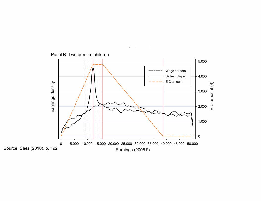
192 AmErICAN ECoNomIC JoUrNAL: ECoNomIC PoLICy AUgUST 2010

systematic clustering around the second kink point of the EITC. Similarly, we cannot discern any gap in the distribution of earnings around the concave kink point where the EITC is completely phased-out. This differential response to the first kink point, versus the other kink points, is surprising in light of the standard model predicting that any convex (concave) kink should produce bunching (gap) in the distribution of earnings.

In Figure 4, we break down the sample of earners into those with nonzero self-employment income versus those zero self-employment income (and hence whose

5,000

4,000

3,000

2,000

1,000

0

5,000

4,000

3,000

2,000

1,000

0

EIC

am

ount

($)

EIC

am

ount

($)

Ear

ning

s de

nsity

0 5,000 10,000 15,000 20,000 25,000 30,000 35,000 40,000 45,000 50,000

Earnings (2008 $)

Wage earners

Self-employed

EIC amount

Panel A. One child

Ear

ning

s de

nsity

0 5,000 10,000 15,000 20,000 25,000 30,000 35,000 40,000 45,000 50,000

Earnings (2008 $)

Panel B. Two or more children

Wage earners

Self-employed

EIC amount

Figure 4. Earnings Density and the EITC: Wage Earners versus Self-Employed

Notes: The figure displays the kernel density of earnings for wage earners (those with no self-employment earnings) and for the self-employed (those with nonzero self employment earnings). Panel A reports the density for tax fil-ers with one dependent child and panel B for tax filers with two or more dependent children. The charts include all years 1995–2004. The bandwidth is $400 in all kernel density estimations. The fraction self-employed in 16.1 per-cent and 20.5 percent in the population depicted on panels A and B (in the data sample, the unweighted fraction self-employed is 32 percent and 40 percent). We display in dotted vertical lines around the first kink point the three bands used for the elasticity estimation with δ = $1,500.


Why not more bunching at kinks?

1) True intensive elasticity of response may be small

2) Randomness in income generation process: Saez (1999)

shows that year-to-year income variation too small to erase

bunching if elasticity is large

3) Frictions: Adjustment costs and institutional constraints

(Chetty, Friedman, Olsen, and Pistaferri QJE’11)

4) Information and salience

44

EITC Behavioral Studies

Strong evidence of response along extensive margin, little ev-idence of response along intensive margin (except for self-employed) ⇒ Possibly due to lack of understanding of theprogram

Qualitative surveys show that:

Low income families know about EITC and understand thatthey get a tax refund if they work

However very few families know whether tax refund ↑ or ↓ withearnings

Such confusion might be good for the government as the EITCinduces work along participation margin without discouragingwork along intensive margin (Liebman-Zeckhauser 2004)

45

Chetty, Friedman, Saez AER’13 EITC heterogeneity

Use US population wide tax return data since 1996 (throughIRS special contract)

1) Substantial heterogeneity in fraction of EITC recipientsbunching (using self-employment) across geographical areas

⇒ Information on EITC varies across areas and grows overtime

2) Places with high self-employment EITC bunching displaywage earnings distribution more concentrated around plateau

3) Omitted variable test: use birth of first child to test causaleff‘EITC on wage earnings

⇒ Evidence of wage earnings response to EITC along intensivemargin

46

0%

2%

4%

6%

8%

Per

cent

of T

ax F

ilers

-$10K $0K $10K $20K $30K

Lowest Bunching Decile Highest Bunching Decile

Total Earnings Relative to First EITC Kink

Earnings Distributions in Lowest and Highest Bunching Deciles

Source: Chetty, Friedman, and Saez NBER'12

4.1 – 42.7% 2.8 – 4.1% 2.1 – 2.8% 1.8 – 2.1% 1.5 – 1.8% 1.2 – 1.5% 1.1 – 1.2% 0.9 – 1.1% 0.7 – 0.9% 0 – 0.7%

Fraction of Tax Filers Who Report SE Income that Maximizes EITC Refund

in 1996


4.1 – 42.7% 2.8 – 4.1% 2.1 – 2.8% 1.8 – 2.1% 1.5 – 1.8% 1.2 – 1.5% 1.1 – 1.2% 0.9 – 1.1% 0.7 – 0.9% 0 – 0.7%


in 1999


4.1 – 42.7% 2.8 – 4.1% 2.1 – 2.8% 1.8 – 2.1% 1.5 – 1.8% 1.2 – 1.5% 1.1 – 1.2% 0.9 – 1.1% 0.7 – 0.9% 0 – 0.7%


in 2002


4.1 – 42.7% 2.8 – 4.1% 2.1 – 2.8% 1.8 – 2.1% 1.5 – 1.8% 1.2 – 1.5% 1.1 – 1.2% 0.9 – 1.1% 0.7 – 0.9% 0 – 0.7%


in 2005


4.1 – 42.7% 2.8 – 4.1% 2.1 – 2.8% 1.8 – 2.1% 1.5 – 1.8% 1.2 – 1.5% 1.1 – 1.2% 0.9 – 1.1% 0.7 – 0.9% 0 – 0.7%


in 2008


0%

0.5%

1%

1.5%

2%

2.5%

3%

3.5%

Per

cent

of W

age-

Ear

ners

$1K

$2K

$3K

$4K

EIT

C A

mou

nt ($

)

$0K

Income Distribution For Single Wage Earners with One Child

W-2 Wage Earnings

Is the EITC having

an effect on this

distribution?

$0 $10K $20K $30K $25K $35K $25K $5K


Lowest Bunching Decile Highest Bunching Decile

W-2 Wage Earnings

Per

cent

of W

age

Ear

ners

EIT

C A

mou

nt ($

)

$0 $10K $20K $30K $25K $35K $25K $5K

Income Distribution For Single Wage Earners with One Child

High vs. Low Bunching Areas

0%

0.5%

1%

1.5%

2%

2.5%

3%

3.5%

$1K

$2K

$3K

$4K

$0K


Earnings Distribution in the Year Before First Child Birth for Wage Earners P

erce

nt o

f Ind

ivid

uals

2%

4%

0%

6%

$0 $30K $40K $10K $20K

Wage Earnings Lowest Sharp Bunching Decile

Middle Sharp Bunching Decile

Highest Sharp Bunching Decile


Earnings Distribution in the Year of First Child Birth for Wage Earners P

erce

nt o

f Ind

ivid

uals

2%

4%

0%

6%

$0 $30K $40K $10K $20K

Wage Earnings Lowest Sharp Bunching Decile

Middle Sharp Bunching Decile

Highest Sharp Bunching Decile


IMPLICATIONS OF ROLE OF INFORMATION

Empirical work:

Information should be a key explanatory variable in estimationof behavioral responses to govt programs

When doing empirical project, always ask the question: didpeople affected understand incentives?

Cannot identify structural parameters of preferences withoutmodeling information and salience

Normative analysis:

Information is a powerful and inexpensive policy tool to affectbehavior

Should be incorporated into optimal policy design problems

48

Value of Administrative data

Key advantages of admin data (in most advanced countries

such as Scandinavia):

1) Size (often full population available)

2) Longitudinal structure (can follow individual across years)

3) Ability to match wide variety of data (tax records, earnings

records, family records, health records, education records)

US is lagging behind in terms of admin data access [hard to

match across agencies]

Private sector also generates valuable big data (Google, Credit

Bureaus, personnel/health data from large companies)

49

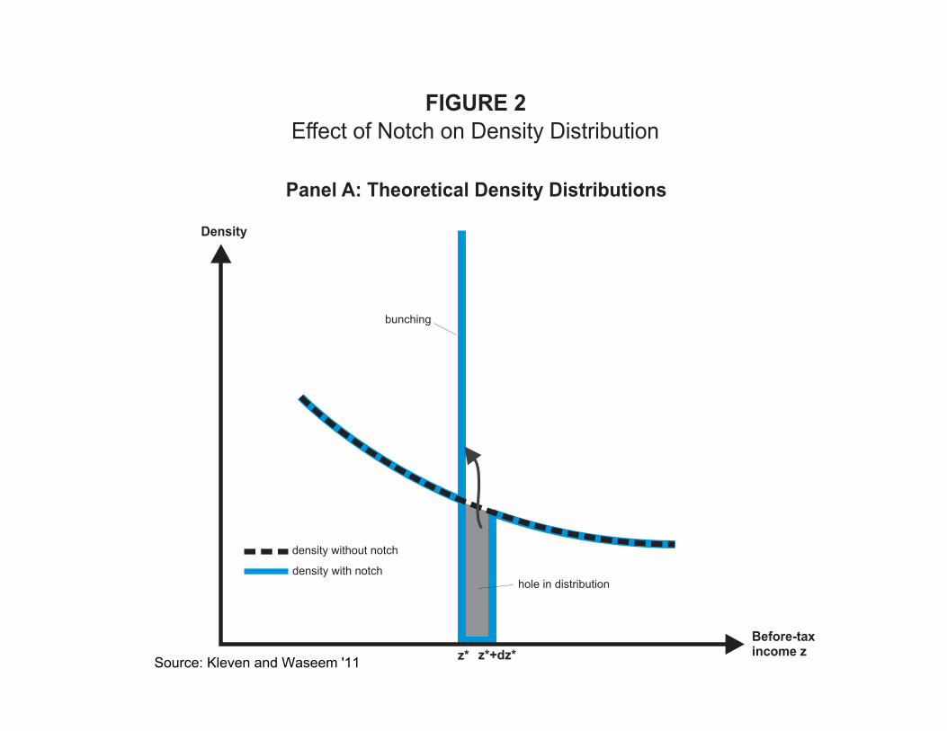
Bunching at Notches

Taxes and transfers sometimes also generate notches (=dis-continuities) in the budget set

Such discontinuities should create bunching (and gaps) in theresulting distributions

Example: Pakistani income tax creates notches because av-

erage tax rate jumps ⇒ Bunching below the notch and gapin density just above the notch

Empirically: Kleven and Waseem QJE’13 find evidence ofbunching (primarily among self-employed) but size of the re-sponse is quantitatively small

Large fraction of taxpayers are unresponsive to notch likelydue to lack of information

50

Notes: thpersonal unincorpRupees (employedto 2006-0earners oshare of self-empconsists a notch,

he figure shoincome tax

orated firms (PKR), and thd applies to t07 and was cor self-emplototal income,loyed individof 21 bracketand the cutof

Person

ows the statuschedules f(blue solid l

he PKR-USDhe full periodchanged by aoyed based o and then tax

duals and firmts (the first 14ff itself belong

nal Income

utory (averagfor wage earine), respect

D exchange ra of this study

a tax reform ion whether inxes total incomms consists 4 of which areg to the tax-fa

FIGURE 3e Tax Sche

ge) tax rate arners (red datively. Taxabate is around

y (2006-08), wn 2008. The ncome from wme accordingof 14 bracke shown in thavored side o

3 edules in P

as a functionashed line) ale income is

d 85 as of Apwhile the schetax system cwages or selg to the assigets, while th

he figure). Eaf the notch.

akistan

n of annual tand self-emp

shown in thpril 2011. Theedule for wagclassifies indivf-employmenned schedulee tax schedch bracket cu

taxable incomployed individhousands of e schedule foge earners apviduals as eitnt constitute te. The tax schdule for wageutoff is assoc

me in the duals and Pakistani r the self-

pplies only ther wage the larger hedule for e earners

ciated with Source: Kleven and Waseem '11

After-taxincome z - T(z)

Before-taxincome z

Individual L

Individual Hslope 1-t

slope 1-t-dt

z* z*+dz*

notch dt·z*

bunching segment

Panel A: Bunching at the Notch

FIGURE 1

After-taxincome z - T(z)

Before-taxincome z

Individual L

Individual Hslope 1-t

slope 1-t-dt

z* z*+dz*

notch dt·z*

bunching segment

B

D

slope 1-t*

Cslope 1-t

Panel B: Comparing the Notch to a Hypothetical Kink

A

Effect of Notch on Taxpayer Behavior

Source: Kleven and Waseem '11

Density

Before-taxincome zz* z*+dz*

density without notch

density with notchhole in distribution

bunching

Density

Before-taxincome zz* z*+δ z*+2δz*-δz*-2δ

h-*

h+*

h0*

H = ·- δ h-* *

H = ·+ δ h+* *

*B = H* - ·hδ 0

FIGURE 2

Effect of Notch on Density Distribution

Panel A: Theoretical Density Distributions

Panel B: Empirical Density Distribution and Bunching Estimation


Notes: thunincorp(shown iincome innumber overtical lijumps by

Self

Panel A: N

Panel C: N

he figure shoorated firms in Figure 3). n even thousof taxpayers ines, and eacy 2.5%-points

Densitf-Employed

Notch at 30

Notch at 50

ows the densin 2006-08 arThe densitie

sands. Each dlocated with

ch notch poins at all the mid

y Distributd Individua

00k

00k

ity distributioround the foues include ondot representhin a 2000 Rnt is itself parddle notches.

FIGURE 5ion around

als and Firm

n of taxable ur middle notcnly “sophisticats the upper b

Rupee range rt of the tax-f.

5 d Middle Noms (Sophis

Pa

Pa

income for mches in the scated filers” debound of a 20below the dofavored side

otches: sticated Fil

anel B: Not

anel D: Not

male self-empchedule applyefined as tho000 Rupee bot. Notch poiof the notch.

lers)

tch at 400k

tch at 600k

ployed individying to those tose who do nbin and thus sints are show. The average

k

k

duals and taxpayers not report shows the wn by red e tax rate


Kleven and Waseem QJE’13 notch analysis

With optimization frictions (lack of information, costs of ad-

justment), a fraction of individuals fail to respond to notch

Kleven-Waseem use empirical density in the theoretical gap

area to measure the fraction of unresponsive individuals

This allows them to back up the frictionless elasticity (i.e. the

elasticity among responsive individuals)

The frictionless elasticity is much higher than the reduced form

elasticity but remains still relatively modest

Additional notch studies: Best and Kleven ’14 on UK housing

purchase tax (stamp duty), Kopczuk-Munroe AEJ’15 on NY-

NJ Mansion tax [also find evidence of bunching responses]

52

Many Recent Bunching Studies

Bunching method applied to many settings with nonlinear bud-gets with convex kink points or notches (Kleven ’16 survey):

• Individual tax (Bastani-Selin ’14 Sweden, Mortenson-Whitten ’16 US)

• Payroll tax (Tazhidinova ’15 on UK)

• Corporate tax (Devereux-Liu-Loretz ’14)

• Health spending (Einav-Finkelstein-Schrimpf ’13 on Medicare Part D)

• Retirement savings (401(k) matches)

• Retirement age (Brown ’13 on California Teachers)

• Housing transactions (Best and Kleven, 2017)

General findings:

(1) clear bunching when information is salient and outcomeeasily manipulable

(2) bunching is almost always small relative to conventionalelasticity estimates

53

Macro Long-Run Evidence

1) Macroeconomists also estimate elasticities by examining

long-term trends/cross-country comparisons

2) Identification more questionable but estimates perhaps more

relevant to long-run policy questions of interest

3) Use aggregate hours data and aggregate measures of taxes

(average tax rates)

4) Highly influential in calibration of macroeconomic models

54

Trend-based Estimates and Macro Evidence

Long-Run: US real wage rates multiplied by about 5 from

1900 to present due to economic growth

Aged 25-54 male hours have fallen 25% and then stabilized

(Ramey and Francis AEJ-macro ’09)

⇒ Uncompensated hours of work elasticity is small (< .1)

However, taxes are rebated as transfers so can still have labor

supply effects if large compensated elasticity/income effects

Alternative plausible story: utility depends on relative con-

sumption ⇒ Earnings $10,000 is low today but would have

been very good in 1900 (reference point labor supply theory)

55

198 AMEricAn EcOnOMic JOUrnAL: MAcrOEcOnOMicS JULy 2009

0

10

20

30

40

50

1900 1920 1940 1960 1980 2000year

0

10

20

30

40

50

1900 1920 1940 1960 1980 2000year

0

10

20

30

40

50

1900 1920 1940 1960 1980 2000year

14−17 18−24

25−54 55−64

651

C. Females

B. Males

A. Both sexes

Figure 2. Average Weekly Hours Worked per Person, by Age Group

Source: Authors’ estimates, based on information from Kendrick (1961, 1973), the census, and the CPS.

Ramey and Francis AEJ'09

Long-run cross-country panel: Prescott 2004

Uses data on hours worked by country in 1970 and 1995 for 7OECD countries [total hours/people age 15-64]

Technique to identify elasticity: calibration of GE model

Rough intuition: posit a labor supply model, e.g.

u(c, l) = c−l1+1/ε

1 + 1/ε

Finds that elasticity of ε = 1.2 best matches time series andcross-sectional patterns

Note that this is analogous to a regression without controlsfor other variables

Results verified in subsequent calibrations by Ohanina-Raffo-Rogerson JME’08 and others using more data

57

Raj Chetty () Labor Supply Harvard, Fall 2009 172 / 227

Reconciling Micro and Macro Estimates

Recent interest in reconciling micro and macro elasticity esti-

mates (see Chetty-Guren-Manoli-Weber ’13)

Three potential explanations

a) Statistical Bias: culture differs in countries with higher tax

rates [Alesina, Glaeser, Sacerdote 2005, Steinhauer 2013 for

Swiss communities by language]

b) Macro-elasticity captures long-term response which could

be larger than short-term response (frictions, etc. Chetty ’12).

c) Other programs: retirement, education affect labor supply

at beginning and end of working life (Blundell-Bozio-Laroque

’11) and child care affecting mothers (Kleven JEP’14)

59

Blundell-Bozio-Laroque ’13

Strong evidence that variation in aggregate hours of work

across countries happens among the young and the old: (a)

schooling-work margin (b) presence of young children (for

women), (c) early retirement

Serious cross-country time series analysis would require to put

together a better tax wedge by age groups which includes all

those additional govt programs [welfare, retirement, child care]

This has been done quite successfully in the case of retirement

by series of books by Gruber and Wise, Retirement around the

world

⇒ Need to develop a more comprehensive international / time

series database of tax wedges by age and family types

60

• There are certain key margins where tax rates impinge on

earnings decisions.

• For many male workers this is at the beginning and at the end

of their working lives. These are the schooling-work margins

and the early retirement margins.

• Indeed much of the difference in male employment across

OECD countries occurs at these points in the life-cycle.

The taxation of income from earnings

Male employment by age – US, FR and UK 2005

0

0.1

0.2

0.3

0.4

0.5

0.6

0.7

0.8

0.9

1

16 18 20 22 24 26 28 30 32 34 36 38 40 42 44 46 48 50 52 54 56 58 60 62 64 66 68 70 72 74 76 78

US

FR

UK

Source Blundell (2009), Mirrlees Review

Male employment by age – US, FR and UK 1975

0

0.1

0.2

0.3

0.4

0.5

0.6

0.7

0.8

0.9

1

16 18 20 22 24 26 28 30 32 34 36 38 40 42 44 46 48 50 52 54 56 58 60 62 64 66 68 70 72 74 76 78

US

FR

UK

Male Hours by age – US, FR and UK 2005

0

200

400

600

800

1000

1200

1400

1600

1800

2000

2200

2400

16 18 20 22 24 26 28 30 32 34 36 38 40 42 44 46 48 50 52 54 56 58 60 62 64 66 68 70 72 74 76 78

US

FR

UK


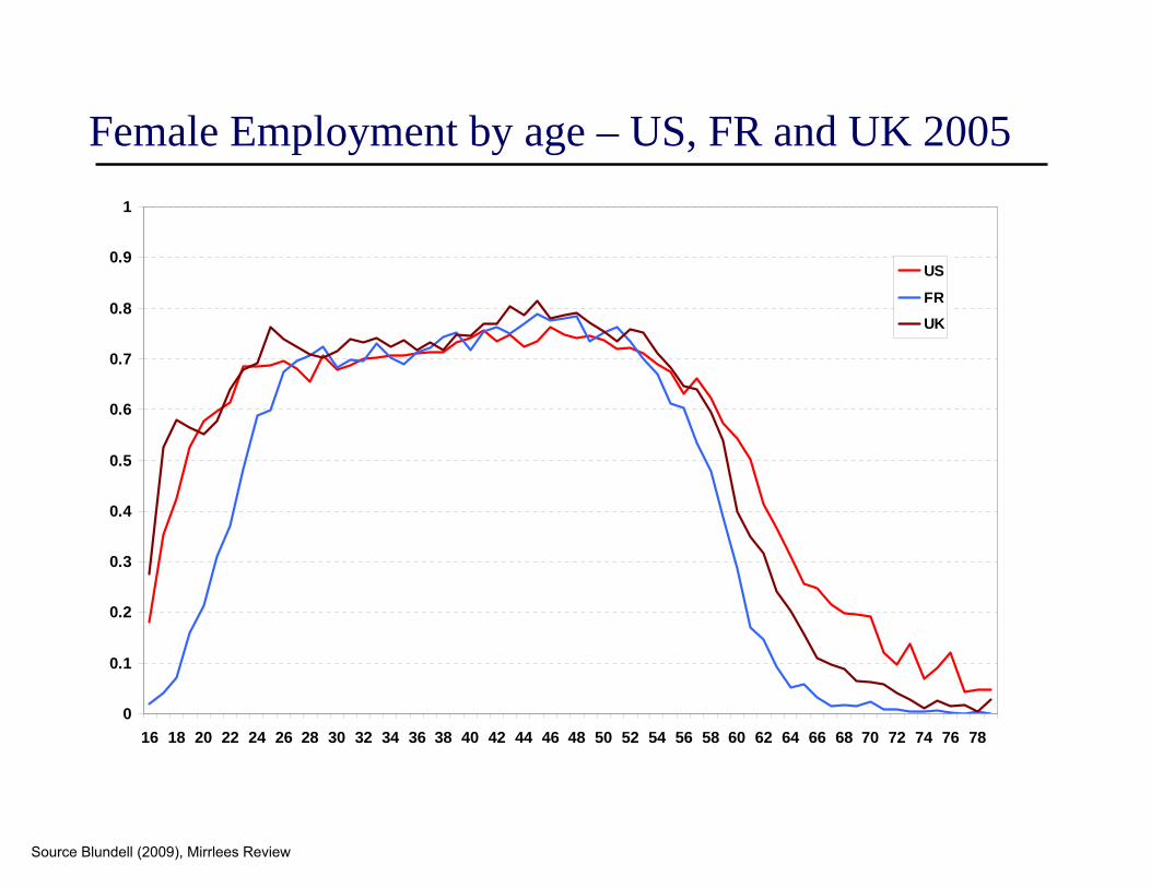
Female Employment by age – US, FR and UK 2005

0

0.1

0.2

0.3

0.4

0.5

0.6

0.7

0.8

0.9

1

16 18 20 22 24 26 28 30 32 34 36 38 40 42 44 46 48 50 52 54 56 58 60 62 64 66 68 70 72 74 76 78

US

FR

UK

Female Hours by age – US, FR and UK 2005

0

200

400

600

800

1000

1200

1400

1600

1800

2000

2200

2400

16 18 20 22 24 26 28 30 32 34 36 38 40 42 44 46 48 50 52 54 56 58 60 62 64 66 68 70 72 74 76 78

US

FR

UK


• For women earnings are influenced by taxes and benefits not

only at these margins but also when there are young children in

the family.

• For women with younger children it is not usually just an

employment decision that is important it is also whether to

work part-time or full-time.

• Often the employment margin is referred to as the extensive

margin of work and the part-time or hours of work decisions

more generally as the intensive margin.

The taxation of income from earnings

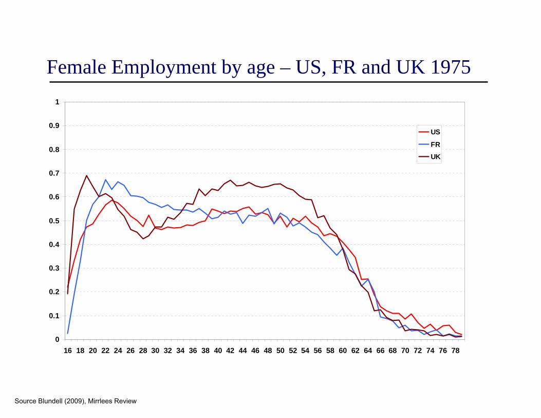
Female Employment by age – US, FR and UK 1975

0

0.1

0.2

0.3

0.4

0.5

0.6

0.7

0.8

0.9

1

16 18 20 22 24 26 28 30 32 34 36 38 40 42 44 46 48 50 52 54 56 58 60 62 64 66 68 70 72 74 76 78

US

FR

UK


Long-term effects: Evidence from the Israeli Kibbutz

Abramitzky ’15 book based on series of academic papers

Kibbutz are egalitarian and socialist communities in Israel,thrived for almost a century within a more capitalist society

1) Social sanctions on shirkers effective in small communitieswith limited privacy

2) Deal with brain drain exit using communal property as abond

3) Deal with adverse selection in entry with screening and trialperiod

4) Perfect sharing in Kibbutz has negative effects on highschool students performance but effect is small in magnitude(concentrated among kids with low education parents)

65

Long-term effects: Evidence from the Israeli Kibbutz

Abramitzky-Lavy ECMA’14 show that high school studentsstudy harder once their kibbutz shifts away from equal sharing

Uses a DD strategy: pre-post reform and comparing reformKibbutz to non-reform Kibbutz. Finds that

1) Students are 3% points more likely to graduate

2) Students are 6% points more likely to achieve a matricula-tion certificate that meets university entrance requirements

3) Students get an average of 3.6 more points in their exams

Effect is driven by students whose parents have low schooling;larger for males; stronger in kibbutz that reformed to greaterdegree

66

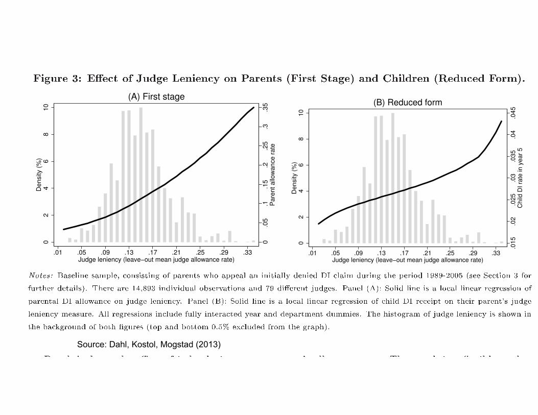
Culture of Welfare across Generations

Conservative concern that welfare promotes a culture of de-pendency: kids growing up in welfare supported families aremore likely to use welfare

Correlation in welfare use across generations is obviously notnecessarily causal

Dahl, Kostol, Mogstad QJE’2014 analyze causal effect ofparental use of Disability Insurance (DI) on children use (asadults) of DI in Norway

Identification uses random assignment of judges to denied DIapplicants who appeal [some judges are severe, some lenient]

Find evidence of causality: parents on DI increases odds ofkids on DI over next 5 years by 6 percentage points

Mechanism seems to be learning about DI availability rather than reducedstigma from using DI [because no effect on other welfare programs use]

67

��

��

��

�� !� �� "�� ##$ ��

� �� %� � �� "�� %$ � ��

��

0.0

5.1

.15

.2.2

5.3

.35

Par

ent a

llow

ance

rat

e

02

46

810

Den

sity

(%

)

.01 .05 .09 .13 .17 .21 .25 .29 .33Judge leniency (leave−out mean judge allowance rate)

(A) First stage

.015

.02

.025

.03

.035

.04

.045

Chi

ld D

I rat

e in

yea

r 5

02

46

810

Den

sity

(%

)

.01 .05 .09 .13 .17 .21 .25 .29 .33Judge leniency (leave−out mean judge allowance rate)

(B) Reduced form

�� ! ��

�� "# $�� %��! ��&�� '��&� �� (� ��)�� *��# +�� ,"- ��

�� *�� # +�� "- �� .� *��

�� # ,�� # $�� *��

�� '��/�� '� � 0�� '� �� #�1 �2�� "#

&�� ' �� (�� )� �� *�"��

� �� +�� ,�� -./� ��

��

�� ' �� )� ��

� � � �� )� �� &�� 0 ��

�� (�� )� �� )� 12 ��

�� )� 12 ��

�� '��"�� -��

�� 3��%� �� / �� 12 +��

� � �� -�� 3 �##�

�� %� � �� /�

�

Source: Dahl, Kostol, Mogstad (2013)

REFERENCES

Abramitzky, Ran The Mystery of the Kibbutz: How Socialism Succeeded,Princeton: Princeton University Press, 2015 (in preparation) (web)

Abramitzky, Ran and Victor Lavy, 2014 “How Responsive is Investment inSchooling to Changes in Redistributive Policies and in Returns?”, Econo-metrica, 82(4), 1241-1272 (web)

Alesina, A., E. Glaeser, and B. Sacerdote “Work and Leisure in the U.S.and Europe: Why So Different?”, NBER Macroeconomics Annual 2005.(web)

Ashenfelter, O. and M. Plant “Non-Parametric Estimates of the LaborSupply Effects of Negative Income Tax Programs”, Journal of Labor Eco-nomics, Vol. 8, 1990, 396-415. (web)

Bastani, Spencer and Hakan Selin, “Bunching and non-bunching at kinkpoints of the Swedish tax schedule,” Journal of Public Economics, 109,2014, 36-49. (web)

Bertrand, M., E. Duflo and S. Mullainhatan “How Much Should we TrustDifferences-in-Differences Estimates?”, Quarterly Journal of Economics,Vol. 119, 2004, 249-275. (web)

69

http://elsa.berkeley.edu/~saez/course/Abramitzky_book_presentation.pdf

http://elsa.berkeley.edu/~saez/course/Abramitzky-Lavy14.pdf

http://www.nber.org/papers/w11278

http://links.jstor.org/stable/pdfplus/2535218.pdf

http://elsa.berkeley.edu/~saez/course/bastani-selin14.pdf


Best, Michael and Henrik Kleven “Housing Market Responses to Transac-tion Taxes: Evidence from Notches and Stimulus in the UK,” Review ofEconomic Studies 2017 forthcoming (web)

Bianchi, M., B. R. Gudmundsson, and G. Zoega. 2001. “Iceland’s Nat-ural Experiment in Supply-Side Economics,” American Economic Review,91(5), 1564-79. (web)

Bitler, M. J. Gelbach and H. Hoynes “What Mean Impacts Miss: Dis-tributional Effects of Welfare Reform Experiments”, American EconomicReview, Vol. 96, 2006, 988-1012. (web)

Bitler, M. and H. Hoynes “The State of the Safety Net in the Post-WelfareReform Era” Brookings Papers on Economic Activity Fall 2010, 71-127(web)

Blau, F. and L. Kahn “Changes in the Labor Supply Behavior of MarriedWomen: 1980-2000”, Journal of Labor Economics, Vol. 25, 2007, 393-438. (web)

Blomquist, S. “Restrictions in labor supply estimation: Is the MaCurdycritique correct?”, Economics Letters, Vol. 47, 1995, 229-235 (web)

Blundell, Richard, Antoine Bozio, and Guy Laroque. 2013. “Extensiveand Intensive Margins of Labour Supply: Work and Working Hours in theUS, UK and France,” Fiscal Studies, 34(1), 1-29 (web)

http://elsa.berkeley.edu/~saez/course/best-kleven_landnotches_may2014.pdf

http://www.jstor.org/stable/pdfplus/2677941.pdf


http://elsa.berkeley.edu/~saez/course/bitler-hoynesBPEA11.pdf

http://www.jstor.org/stable/pdfplus/10.1086/513416.pdf

http://elsa.berkeley.edu/~saez/course/Blomquist_EL(1995).pdf

http://elsa.berkeley.edu/~saez/course/blundell-bozio-laroque11labor.pdf

Blundell, R., A. Duncan and C. Meghir “Estimating Labor Supply Re-sponses Using Tax Reforms”, Econometrica, Vol. 66, 1998, 827-862.(web)

Blundell, R. and T. MaCurdy “Labor supply: a review of alternative ap-proaches”, in the Handbook of Labor Economics, Vol. 3A, O. Ashenfelterand D. Card, eds. Amsterdam: Elsevier Science 1999. (web)

Brown, K. “The Link between Pensions and Retirement Timing: Lessonsfrom California Teachers”, Journal of Public Economics, 98, 2013, 1–14.2007 (web)

Camerer, C., L. Babcock, G. Loewenstein and R. Thaler “Labor Supplyof New York City Cabdrivers: One Day at a Time”, Quarterly Journal ofEconomics, Vol. 112, 1997, 407-441. (web)

Card, David, Raj Chetty, Martin Feldstein, and Emmanuel Saez “Expand-ing Access to Administrative Data for Research in the United States,”White Paper for NSF 10-069 call for papers on ”Future Research in theSocial, Behavioral, and Economic Sciences” September 2010. (web)

Card, D.,R. Chetty, and A. Weber, “Cash-on-Hand and Competing Mod-els of Intertemporal Behavior: New Evidence from the Labor Market”,Quarterly Journal of Economics, Vol. 122, 2007, 1511-1560. (web)


http://elsa.berkeley.edu/~saez/course/Blundell-MaCurdy_Handbook.pdf

http://elsa.berkeley.edu/~saez/course/brown_jpube13.pdf


http://elsa.berkeley.edu/~saez/card-chetty-feldstein-saezNSF10dataaccess.pdf

http://elsa.berkeley.edu/~saez/course/Card,Chetty,Weber_QJE(2007).pdf

Card, David, and Dean R. Hyslop. 2005. “Estimating the Effects of aTime-Limited Earnings Subsidy for Welfare-Leavers” Econometrica, 73(6),1723-70. (web)

Cesarini, David, Erik Lindqvist, Matthew J. Notowidigdo, Robert Ostling.2015 “The Effect of Wealth on Individual and Household Labor Supply:Evidence from Swedish Lotteries”, NBER Working Paper No. 21762.(web)

Chetty, R. “A New Method of Estimating Risk Aversion”, The AmericanEconomic Review, Vol. 96, 2006, 1821-1834. (web)

Chetty, Raj. 2012. “Bounds on Elasticities with Optimization Frictions: ASynthesis of Micro and Macro Evidence on Labor Supply,” Econometrica80(3), 969–1018. (web)

Chetty, R., Adam Guren, Day Manoli, and Andrea Weber. 2013 “DoesIndivisible Labor Explain the Difference between Micro and Macro Elastic-ities? A Meta-Analysis of Extensive Margin Elasticities”, NBER Macroe-conomics Annual, University of Chicago Press, 27(1), 1–56. (web)

Chetty, R., J. Friedman, T. Olsen and L. Pistaferri “Adjustment Costs,Firms Responses, and Micro vs. Macro Labor Supply Elasticities: Evidencefrom Danish Tax Records”, Quarterly Journal of Economics, 126(2), 2011,749-804. (web)


http://www.nber.org/papers/w21762.pdf


http://elsa.berkeley.edu/~saez/course/chettyEMA12.pdf

http://elsa.berkeley.edu/~saez/course/chettyetal2013NBERmacro.pdf

http://elsa.berkeley.edu/~saez/course/chettyetalQJE2011denmark.pdf

Chetty, R., J. Friedman and E. Saez “Using Differences in Knowl-edge Across Neighborhoods to Uncover the Impacts of the EITC onEarnings”, American Economic Review, 2013, 103(7), 2683-2721(web)

Chetty, R. and E. Saez “Teaching the Tax Code: Earnings Responsesto an Experiment with Recipients”, American Economic Journal: AppliedEconomics 5(1), 2013, 1-31. (web)

Crawford, V. and J. Meng “New York City Cabdrivers’ Labor Supply Revis-ited: Reference-Dependence Preferences with Rational-Expectations Tar-gets for Hours and Income”, University of California at San Diego, Eco-nomics Working Paper Series: 2008-03, 2008. (web)

Dahl, Gordon B., Andreas Ravndal Kostol, Magne Mogstad “FamilyWelfare Cultures” Quarterly Journal of Economics, 129(4), 2014,1711-52 (web)

Davis, J. and M. Henrekson, “Tax Effects on Work Activity, Industry Mixand Shadow Economy Size: Evidence from Rich Country Comparisons”,in R. Gomez-Salvador, A. Lamo, B. Petrongolo, M. Ward and E. Wasmereds., Labour Supply and Incentives to Work in Europe, 2005, 44-104.(web)

Devereux, Michael P, Li Liu and Simon Loretz. 2014. ”The Elasticityof Corporate Taxable Income: New Evidence from UK Tax Records.”American Economic Journal: Economic Policy, 6(2): 19-53. (web)

http://eml.berkeley.edu/~saez/chetty-friedman-saezAER13EITC.pdf

http://elsa.berkeley.edu/~saez/chetty-saezAEJ13EITC.pdf

http://elsa.berkeley.edu/~saez/course/Crawford,Meng(2009).pdf

http://elsa.berkeley.edu/~saez/course/dahl-kostol-mogstadQJE14.pdf


http://elsa.berkeley.edu/~saez/devereuxetal13.pdf

Einav, Liran, Amy Finkelstein, Paul Schrimpf “The Data Revolution andEconomic Analysis’, NBER Working Paper 19035, 2013. (web)

Einav, Liran and Jonathan Levin “The Data Revolution and EconomicAnalysis”, NBER Working Paper No. 19035, 2013 (web)

Eissa, N. and H. Hoynes “Taxes and the labor market participation of mar-ried couples: the earned income tax credit”, Journal of Public Economics,Vol. 88, 2004, 1931-1958. (web)

Eissa, N. and J. Liebman “Labor Supply Response to the Earned IncomeTax Credit”, Quarterly Journal of Economics, Vol. 111, 1996, 605-637.(web)

Farber, H. “Is Tomorrow Another Day? The Labor Supply of New YorkCity Cab Drivers”, Journal of Political Economy, Vol. 113, 2005, 46-82.(web)

Farber, H. “Reference-Dependent Preferences and Labor Supply: TheCase of New York City Taxi Drivers”, The American Economic Review,Vol. 98, 2008, 1069-1082. (web)

Fehr, E. and L. Goette “Do Workers Work More if Wages Are High? Evi-dence from a Randomized Field Experiment”, American Economic Review,Vol. 97, 2007, 298-317. (web)



http://elsa.berkeley.edu/~saez/course/Eissa and Hoynes_JPubE(2004).pdf





Friedberg, L. “The Labor Supply Effects of the Social Security EarningsTest”, Review of Economics and Statistics, Vo. 82, 2000, 48-63. (web)

Greenberg, D. and H. Hasley, “Systematic Misreporting and Effects ofIncome Maintenance Experiments on Work Effort: Evidence from theSeattle-Denver Experiment”, Journal of Labor Economics, Vol. 1, 1983,380-407. (web)

Hausman, J. “Stochastic Problems in the Simulation of Labor Supply”,NBER Working Paper No. 0788, 1981. (web)

Hausman, J. “Taxes and Labor Supply”, in A. Auerbach and M. Feldstein,eds, Handbook of Public Finance, Vol I, North Holland 1987. (web)

Heckman, J. “What Has Been Learned About Labor Supply in the PastTwenty Years?”, American Economic Review, Vol. 83, 1993, 116-121.(web)

Heckman, J. and M. Killingsworth “Female Labor Supply: A Survey” Hand-book of Labor Economics, Vol. I, Chapter 2, 1986. (web)

Hotz, J. and K. Scholz “The Earned Income Tax Credit”, NBER WorkingPaper No. 8078, 2001. (web)




http://elsa.berkeley.edu/~saez/course/Hausman_Handbook.pdf


http://elsa.berkeley.edu/~saez/course/Heckman and Killingsworth_Handbook.pdf


Imbens, G.W., D.B. Rubin and B.I. Sacerdote “Estimating the Ef-fect of Unearned Income on Labor Earnings, Savings, and Con-sumption: Evidence from a Survey of Lottery”, American EconomicReview, Vol. 91, 2001, 778-794. (web)

Jones, Damon “Information, Inertia and Public Benefit Participation: Ex-perimental Evidence from the Advance EITC and 401(k) Savings“, AEJ:Applied Economics, Vol. 2, 2010, 147-163. (web)

Keane, Michael “Labor Supply and Taxes: A Survey?”, Journal of Eco-nomic Literature, Vol. 49(4), 2011, 961-1075. (web)

Kleven, Henrik “How Can Scandinavians Tax So Much?”, Journal of Eco-nomic Perspectives 28(4), 77-98, 2014 (web)

Kleven, Henrik “Bunching”, Annual Review of Economics, 8, 2016,435-464. (web)

Kleven, Henrik and Mazhar Waseem, 2013“Using notches to uncover op-timization frictions and structural elasticities: Theory and evidence fromPakistan”, Quarterly Journal of Economics 2013, 669-723. (web)

Kline, Patrick and Melissa Tartari, 2016. ”Bounding the Labor SupplyResponses to a Randomized Welfare Experiment: A Revealed PreferenceApproach,” American Economic Review, 106(4), 972-1014. (web)


http://elsa.berkeley.edu/~saez/course/Jones_AEJ.pdf

http://elsa.berkeley.edu/~saez/course/keaneJEL11laborsupply.pdf

http://pubs.aeaweb.org/doi/pdfplus/10.1257/jep.28.4.77

http://elsa.berkeley.edu/~saez/course/kleven_annualreview.pdf

http://elsa.berkeley.edu/~saez/course/kleven-waseemQJE13.pdf

http://elsa.berkeley.edu/~saez/course/klinetkopartari13.pdf

Kopczuk, Wojciech and David J. Munroe, 2015 “Mansion Tax: The Ef-fect of Transfer Taxes on the Residential Real Estate Market”, AmericanEconomic Journal: Economic Policy, 7(2), 214-57 (web)

Liebman, J. and R. Zeckhauser “Schmeduling”, Harvard University workingpaper, October 2004. (web)

MaCurdy, T. “An Empirical Model of Labor Supply in a Life-Cycle Set-ting”, Journal of Political Economy, Vol. 89, 1981, 1059-1085. (web)

MaCurdy, T. “A Simple Scheme for Estimating an Intertemporal Model ofLabor Supply and Consumption in the Presence of Taxes and Uncertainty”,International Economic Review, Vol. 24, 1983, 265-289. (web)

MaCurdy, T., D. Green and H. Paarsch “Assessing Empirical Approachesfor Analyzing Taxes and Labor Supply” Journal of Human Resources, Vol.25, 1990, 415-490. (web)

Meyer, B. and D. Rosenbaum “Welfare, the Earned Income Tax Credit,and the Labor Supply of Single Mothers”, Quarterly Journal of Economics,Vol. 116, August 2001, 1063-1114. (web)

Meyer, B. and X. Sullivan “The effects of welfare and tax reform: thematerial well-being of single mothers in the 1980s and 1990s”, Journal ofPublic Economics, Vol. 88, 2004, 1387-1420. (web)

http://elsa.berkeley.edu/~saez/course/kopczuk-munroe15.pdf

http://elsa.berkeley.edu/~saez/course/schmeduling-zeckhauser.pdf





http://elsa.berkeley.edu/~saez/course/Meyer and Sullivan_JPubE(2004).pdf

Moffitt, R. “Welfare Programs and Labor Supply”, in A. Auerbach and M.Feldstein, Handbook of Public Economics, Volume 4, Chapter 34, Ams-terdam: North Holland, 2003. (web)

Mortenson, Jacob A. and Andrew Whitten. 2016. “Bunching to MaximizeTax Credits: Evidence from Kinks in the U.S. Tax Schedule”, OTA-JCTworking paper (web)

Mroz, T. “The Sensitivity of An Empirical Model of Married Women’sHours of Work to Economic and Statistical Assumptions”, Econometrica,Vol. 55, 1987, 765-799. (web)

Munnell, A., Lessons from the income maintenance experiments : proceed-ings of a conference held at Melvin Village, New Hampshire, September1986. Boston: Federal Reserve Bank of Boston, 1986. (web)

Nichols, Austin and Jesse Rothstein 2015. “The Earned Income TaxCredit”, forthcoming in Volume on US Transfer Programs edited by R.Moffitt (web)

Oettinger, G. “An Empirical Analysis of the Daily Labor Supply of StadiumVendors”, Journal of Political Economy, Vol. 107, 1999, 360-392. (web)

Ohanian, L., A. Raffo, and R. Rogerson “Long-Term Changes in LaborSupply and Taxes: Evidence from OECD Countries, 1956-2004”, Journalof Monetary Economics, Vol. 55, 2008, 1353-1362. (web)

http://elsa.berkeley.edu/~saez/course/Moffitt_Handbook.pdf

http://elsa.berkeley.edu/~saez/course/mortenson-whitten16bunching.pdf


http://elsa.berkeley.edu/~saez/course/Munnell(1986)book.pdf

http://elsa.berkeley.edu/~saez/course/nichols-rothstein-draft_Nov2014.pdf


http://elsa.berkeley.edu/~saez/course/Ohanianetal(2008).pdf

Pencavel, J. “Labor Supply of Men: A Survey”, Handbook of Labor Eco-nomics, vol. 1, chapter 1, 1986. (web)

Pencavel, J. “A Cohort Analysis of the Association between Work Hoursand Wages among Men”, The Journal of Human Resources, Vol. 37,2002, 251-274. (web)

Prescott, E. “Why Do Americans Work So Much More Than Europeans?”,NBER Working Paper No. 10316, 2004, published in FRB Minneapolis -Quarterly Review, 2004, 28(1), 2-14. (web)

Prescott, E. “Nobel Lecture: The Transformation of Macroeconomic Pol-icy and Research”, Journal of Political Economy, 114, 2006, 203-235.(web)

Ramey, Valerie A. and Neville Francis, 2009. “A Century of Work andLeisure,” American Economic Journal: Macroeconomics, 1(2), 189-224.(web)

Rees, A. “An Overview of the Labor-Supply Results”, The Journal ofHuman Resources, Vol. 9, 1974, 158-180. (web)

Rogerson, R. and J. Wallenius “Micro and Macro Elasticities in a LifeCycle Model with Taxes”, Journal of Economic Theory, Vol. 144, 2009,2277-2292. (web)

http://elsa.berkeley.edu/~saez/course/Pencavel_Handbook.pdf




http://elsa.berkeley.edu/~saez/course/ramey-francisAEJ09laborsupply.pdf


http://elsa.berkeley.edu/~saez/course/Rogerson_JET(2009).pdf

Rothstein, J. ‘Is the EITC as Good as an NIT? Conditional Cash Transfersand Tax Incidence.” American Economic Journal: Economic Policy 2 (1),February 2010, 177-208. (web)

Saez, E. “Do Taxpayers Bunch at Kink Points?”, NBER Working PaperNo. 7366, 1999. (web)

Saez, E. “Do Taxpayers Bunch at Kink Points?”, AEJ: EconomicPolicy, Vol. 2, 2010, 180-212. (web)

Saez, E., J. Slemrod, and S. Giertz “The Elasticity of Taxable Income withRespect to Marginal Tax Rates: A Critical Review”, Journal of EconomicLiterature 50(1), 2012, 3-50. (web)

Steinhauer, Andreas “Identity, Working Moms, and Childlessness: Evidencefrom Switzerland”, Working Paper, 2013.(web)

http://elsa.berkeley.edu/~saez/course/rothsteinAEJ10.pdf


http://elsa.berkeley.edu/~saez/course/Saez_AEJ(2010).pdf

http://elsa.berkeley.edu/~saez/saez-slemrod-giertzJEL12.pdf

http://elsa.berkeley.edu/~saez/course/steinhauer.pdf

230B: Public Economics Labor Supply Responses to …saez/course/Labortaxes/laborsupply/labor...230B:...

Documents

Transcript of 230B: Public Economics Labor Supply Responses to …saez/course/Labortaxes/laborsupply/labor...230B:...