226 A PANEL DATA APPRO) - Unisa
160
FOREIGN DIRECT INVESTMENT INFLOWS AND ECONOMIC GROWTH IN SADC COUNTRIES – A PANEL DATA APPROACH by EDMORE MAHEMBE submitted in accordance with the requirements for the degree of MASTER OF COMMERCE in the subject ECONOMICS at the University of South Africa Supervisor: PROF NICHOLAS M. ODHIAMBO Pretoria August 2014
Transcript of 226 A PANEL DATA APPRO) - Unisa

FOREIGN DIRECT INVESTMENT INFLOWS
AND ECONOMIC GROWTH IN SADC
COUNTRIES – A PANEL DATA APPROACH
by
EDMORE MAHEMBE
submitted in accordance with the requirements for the degree of
MASTER OF COMMERCE
in the subject
ECONOMICS
at the
University of South Africa
Supervisor: PROF NICHOLAS M. ODHIAMBO
Pretoria
August 2014

ii
Foreign Direct Investment Inflows and Economic Growth in
SADC Countries – A Panel Data Approach
By
Edmore Mahembe
Degree: Master of Commerce
Department: Economics
Promoter: Prof N. M. Odhiambo

iii
Student number: 47193573
DECLARATION
I declare that Foreign Direct Investment Inflows and Economic Growth in SADC Countries –
A Panel Data Approach is my own work and that all the sources that I have used or quoted have
been indicated and acknowledged by means of complete references.
................................... ...................................
E. Mahembe (Mr.) Date

iv
DEDICATION
This dissertation is dedicated to my God: the Father, the Son and the Holy Spirit; my parents Mr.
B. H. Mahembe and Mrs. R. Mahembe; my wife Maria Nhlanhla Mahembe; and our children
Rachel Rumbidzai Mahembe and Michael Anesu Mahembe.

v
ACKNOWLEDGEMENTS
I would like to express my sincere gratitude and appreciation to all those who assisted me in
completing this dissertation. So many people contributed in motivating, influencing, guiding,
supporting and encouraging me, but owing to space constraints I will mention a few.
Special appreciation goes to my supervisor, Prof. N. M. Odhiambo for his guidance and support.
His availability for comments, even at very late hours was a big encouragement and inspiration.
I’m grateful to my parents Mr. and Mrs. Mahembe for instilling discipline in me; my wife Maria
for the limitless support and encouragement; our children Rachel Rumbidzai and Michael Anesu
for their patience; and the rest of my family and friends for their love and kindness.
I am forever grateful to my pastors; Pastor Andrew and Pastor Bernadette Mutondoro for building
me up and shepherding me and my family with great love.
My profound appreciation goes to the Almighty God, who is my Rock and Strength. The Lord has
lavished me with His grace and favour.
Notwithstanding the guidance and contribution from the aforementioned individuals, the
responsibility for all the views and any shortcomings is entirely mine.

vi
ABSTRACT
This dissertation examines the causal relationship between inward foreign direct investment (FDI)
and economic growth (GDP) in SADC countries. The study investigates, within a panel data
context, whether causation is short-term, long-term or both; and explores whether the causal
relationship between the two variables differs according to income level. The study covered a
panel of 15 SADC countries over the period 1980-2012. In order to assess whether the causal
relationship between FDI inflows and economic growth is dependent on the level of income, the
study divided the SADC countries into two groups, namely, the low-income and the middle-
income countries. The study used the recently developed panel data analysis methods to examine
this causal relationship. It adopted a three stage approach, which consists of panel unit root, panel
cointegration and Granger causality to examine the dynamic causal relationship between the two
variables. Panel unit root results show that both variables in the two SADC country groups were
integrated of order one. Panel cointegration tests showed that the variables for low-income
country group were not cointegrated, while the variables for the middle-income countries were
cointegrated. Since the low-income country group panels were not cointegrated, Granger-
causality tests were conducted within a VAR framework, while causality tests for the middle-
income country group were conducted within an ECM framework. Panel Granger causality results
for the low-income countries showed no evidence of causality in either direction. However, for
the middle-income countries’ panel, there was evidence of a unidirectional causal flow from GDP
to FDI in both the long- and short- run. The study concludes that the FDI-led growth hypothesis
does not apply to SADC countries. The results imply that the recent high economic growth rates
recorded in the SADC region, especially middle-income countries, have been attracting FDI. In
other words, it is economic growth that drives FDI inflows into the SADC region, and not vice
versa. These findings have profound policy implications for the SADC region at large and
individual countries.
Key Terms: Foreign direct investment, economic growth, SADC, error correction model (ECM),
vector autoregressions (VAR), panel data, Granger causality, unit root, and cointegration.
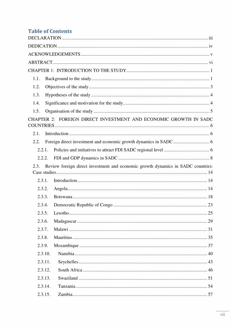
vii
Table of Contents
DECLARATION ............................................................................................................................. iii
DEDICATION ................................................................................................................................. iv
ACKNOWLEDGEMENTS .............................................................................................................. v
ABSTRACT ..................................................................................................................................... vi
CHAPTER 1: INTRODUCTION TO THE STUDY ....................................................................... 1
1.1. Background to the study ..................................................................................................... 1
1.2. Objectives of the study ....................................................................................................... 3
1.3. Hypotheses of the study ..................................................................................................... 4
1.4. Significance and motivation for the study.......................................................................... 4
1.5. Organisation of the study ................................................................................................... 5
CHAPTER 2: FOREIGN DIRECT INVESTMENT AND ECONOMIC GROWTH IN SADC
COUNTRIES .................................................................................................................................... 6
2.1. Introduction ........................................................................................................................ 6
2.2. Foreign direct investment and economic growth dynamics in SADC ............................... 6
2.2.1. Policies and initiatives to attract FDI SADC regional level ....................................... 6
2.2.2. FDI and GDP dynamics in SADC .............................................................................. 8
2.3. Review foreign direct investment and economic growth dynamics in SADC countries:
Case studies ................................................................................................................................. 14
2.3.1. Introduction ............................................................................................................... 14
2.3.2. Angola ....................................................................................................................... 14
2.3.3. Botswana ................................................................................................................... 18
2.3.4. Democratic Republic of Congo ................................................................................ 23
2.3.5. Lesotho ...................................................................................................................... 25
2.3.6. Madagascar ............................................................................................................... 29
2.3.7. Malawi ...................................................................................................................... 31
2.3.8. Mauritius ................................................................................................................... 35
2.3.9. Mozambique ............................................................................................................. 37
2.3.10. Namibia ................................................................................................................. 40
2.3.11. Seychelles .............................................................................................................. 43
2.3.12. South Africa .......................................................................................................... 46
2.3.13. Swaziland .............................................................................................................. 51
2.3.14. Tanzania ................................................................................................................ 54
2.3.15. Zambia ................................................................................................................... 57

viii
2.3.16. Zimbabwe .............................................................................................................. 61
2.4. Conclusion ........................................................................................................................ 65
CHAPTER 3: THEORETICAL AND EMPIRICAL LITERATURE REVIEW ........................... 67
3.1. Introduction ...................................................................................................................... 67
3.2. FDI and economic growth: Theoretical considerations ................................................... 67
3.2.1. Definition of FDI ...................................................................................................... 67
3.2.2. Theoretical relationship between FDI and economic growth ................................... 70
3.2.3. Causal relationship between FDI and economic growth .......................................... 79
3.3. Empirical review on the causality between FDI and GDP............................................... 80
3.3.1. Initial considerations ................................................................................................. 80
3.3.2. Studies which used time series data .......................................................................... 81
3.3.3. Studies which used cross sectional data.................................................................... 86
3.3.4. Studies which used panel data .................................................................................. 87
3.4. Conclusion ........................................................................................................................ 92
CHAPTER 4: PRESENTATION OF THE METHODOLOGY .................................................... 95
4.1. Introduction ...................................................................................................................... 95
4.2. Justification for using panel data ...................................................................................... 95
4.3. Empirical model specification .......................................................................................... 96
4.3.1. Standard Granger causality test ................................................................................ 97
4.3.2. Vector Autoregressions (VAR) ................................................................................. 97
4.3.3. Error correction model (ECM).................................................................................. 99
4.4. Data sources and definitions of variables ....................................................................... 100
4.5. Panel unit roots tests: Review of recent literature .......................................................... 101
4.5.1. Levin, Lin and Chu (LLC) (2002) .......................................................................... 101
4.5.2. IM, Pesaran and Shin (IPS) (2003) ......................................................................... 102
4.5.3. Breitung (2000) test ................................................................................................ 103
4.5.4. Fisher-ADF and Fisher-PP [Madala and Wu (1999) and Choi (2001)] tests ......... 104
4.5.5. Hadri (2000) test ..................................................................................................... 105
4.6. Panel cointegration tests: Review of recent literature .................................................... 107
4.6.1. Residual-Based DF and ADF tests (Kao, 1999) ..................................................... 107
4.6.2. Panel ADF and PP tests (McCoskey and Kao, 2001) ............................................. 108
4.6.3. Pedroni (1999, 2004) panel cointegration tests....................................................... 108
4.6.4. Johansen and Fisher panel cointegration tests (Madala and Wu, 1999). ................ 109

ix
CHAPTER 5: EMPIRICAL ANALYSIS OF THE CAUSAL RELATIONSHIP BETWEEN FDI
AND ECONOMIC GROWTH IN SADC COUNTRIES ............................................................. 111
5.1. Introduction .................................................................................................................... 111
5.2. Descriptive analysis........................................................................................................ 111
5.3. Presentation and interpretation of panel unit roots tests results ..................................... 116
5.4. Panel cointegration test results ....................................................................................... 117
5.5. Presentation and interpretation of panel causality test results........................................ 119
5.5.1. Low income countries ............................................................................................. 119
5.5.2. Middle income countries......................................................................................... 120
CHAPTER 6: CONCLUSION AND POLICY IMPLICATIONS ............................................... 123
6.1. Introduction .................................................................................................................... 123
6.2. Summary of the study .................................................................................................... 123
6.3. Summary and discussion of empirical findings ............................................................. 125
6.4. Policy implications and recommendations ..................................................................... 126
6.5. Limitations of the study and suggestions for further research ....................................... 127
BIBLIOGRAPHY ......................................................................................................................... 128
APPENDICES .............................................................................................................................. 148
List of Tables
Table 1: SADC Comparison with other African Regional Blocs (2011) ......................................... 8
Table 2: Phases of Economic Development Trajectory in Zambia ................................................ 58
Table 3: Summary of Empirical Studies using Time Series Type of Data ..................................... 84
Table 4: Summary of Empirical Studies on Panel Data ................................................................. 90
Table 5: Variables used in this study ............................................................................................ 100
Table 6: Descriptive statistics of variables ................................................................................... 112
Table 7: Panel Unit Root Tests by SADC Country Groups.......................................................... 116
Table 8: Panel Unit Root Tests by SADC Country Groups (First Difference) ............................ 117
Table 9: Pedroni Panel Cointegration Tests for FDI and GDP for SADC countries groups ........ 118
Table 10: Kao (1999) Panel cointegration test by SADC country group ..................................... 119
Table 11: Panel Granger causality tests of FDI and GDP in low income SADC countries ......... 120
Table 12: Panel Granger causality tests results for middle income countries .............................. 121

x
List of Figures
Figure 1: Share of SADC Total GDP, 2011 ..................................................................................... 9
Figure 2: Share of total FDI (1980-2011) ....................................................................................... 10
Figure 3: Total FDI in million US$ (1980-2011) ........................................................................... 11
Figure 4: FDI and GDP Dynamics in the SADC Region ............................................................... 12
Figure 5: FDI into SADC countries by Top 20 Source Countries -Jan 03 - Apr 13 (US$m) ......... 13
Figure 6: FDI into SADC Top 20 Sectors between Jan 03 - Apr 13 (US$m) ................................ 14
Figure 7: Angola GDP and FDI (1980-2012) ................................................................................. 16
Figure 8: FDI Inflows in Angola (USD at current prices and current exchange rates in millions) 17
Figure 9: Botswana GDP and FDI Trends (1980-2011) ................................................................. 21
Figure 10: Levels of FDI in Botswana by Industry (2011) ............................................................. 22
Figure 11: DRC GDP and FDI Trends (1980-2011) ...................................................................... 24
Figure 12: Lesotho GDP and FDI (1980-2011) .............................................................................. 27
Figure 13: GDP and FDI Trends in Madagascar, 1980-2011 ......................................................... 30
Figure 14: GDP and FDI Trends in Malawi, 1980-2011 ................................................................ 34
Figure 15: GDP and FDI Trends in Mauritius (1980-2011) ........................................................... 36
Figure 16: GDP and FDI Trends in Mozambique (1980-2011) ..................................................... 39
Figure 17: GDP and FDI Trends in Namibia (1980-2011) ............................................................. 42
Figure 18: GDP and FDI Trends in Seychelles (1980-2011) ......................................................... 45
Figure 19: Structure of the South African Economy ...................................................................... 48
Figure 20: South Africa GDP and FDI Trends (1980-2011) .......................................................... 49
Figure 21: GDP and FDI Trends in Swaziland (1980-2011) .......................................................... 53
Figure 22: GDP and FDI Trends in Tanzania (1980-2011) ............................................................ 56
Figure 23: GDP and FDI Trends in Zambia (1980-2011) .............................................................. 60
Figure 24: Zimbabwe GDP and FDI Trends (1980-2011).............................................................. 64
Figure 25: FDI Stock in Middle Income Countries 1980-2012 (US Millions)............................. 112
Figure 26: Real GDP in Middle Income Countries 1980-2012 (US Millions) ............................. 113
Figure 27: FDI Stock in Low Income Countries 1980-2012 (US Millions) ................................. 114
Figure 28: Real GDP in Low Income Countries 1980-2012 (US Millions) ................................. 115

1
CHAPTER 1: INTRODUCTION TO THE STUDY
1.1. Background to the study
Both theoretical and empirical literature reveal that foreign direct investment (FDI), which is defined as
international investment by an entity resident in one economy in the business of an enterprise resident in
another economy that is made with the objective of obtaining a lasting interest (IMF, 1993), can contribute
to economic growth. In theory, FDI can boost the host country’s economy via capital accumulation by the
introduction of new goods and foreign technology, and by enhancing a stock of knowledge in the host
country via the transfer of skills (Elboiashi, 2011).
Herzer, Klasen, and Nowak-Lehmann (2008) highlight the fact that FDI plays an important function in host
countries’ economic growth by increasing investible capital and technological spillovers. OECD (2002:5)
further argues that FDI represents a potential source for sustainable growth and development, given its
assumed ability to: (i) Generate technology spillovers; (ii) assist in human capital formation and
development; (iii) help host countries to integrate into the global economy trade; (iv) assist in creating a
more competitive business environment; and (v) enhance the development of enterprise.
According to Dupasquier and Osakwe (2005), FDI complements domestic savings by bestowing foreign
savings. Ndoricimpa (2009:34) further argues that FDI fills the funding gap between local savings and
investment requirements, and can also augment the host country’s balance-of-payment receipts. The United
Nations Conference on Trade and Development (UNCTAD) also argues that FDI is a more stable source of
funding, since it is based on a longer-term view of the recipient country’s growth potential, raw material
accessibility, and access to markets (UNCTAD, 1999).
As a result of these perceived benefits, individual countries and regional blocs across the world have been
actively pursuing policies to attract FDI. Increase in FDI flows has become a global phenomenon. Collier,
Dollar and World Bank (2002) noted that the new wave of financial globalisation started in the early
1980s. Global FDI flows grew from US$50 billion in the early 1980s to US$1.5 trillion in 2011. Africa and
the Southern African Development Community (SADC) region have also witnessed a substantial increase
in FDI inflows. For the SADC1, FDI inflows have grown by almost fifty times in the last three decades;
from a mere US$372 million in 1980 to US$18 billion in 2008. Although FDI inflows to SADC decreased
to US$8 billion in 2010, there are signs of recovery as the inflows grew by 63% to US$13 billion in 2011
(UNCTAD, 2011b and 2012).
1 SADC 15 Member States are Angola, Botswana, Democratic Republic of the Congo (DRC), Lesotho, Madagascar,
Malawi, Mauritius, Mozambique, Namibia, Seychelles, South Africa Swaziland, Tanzania, Zambia, and Zimbabwe.

2
Africa in general and SADC in particular, owing to inadequate resources to finance long-term
development, have been looking at FDI to boost economic growth and reduce poverty in line with the
Millennium Development Goals (MDGs) by 2015. At a continental level, African leaders developed a
programme; the New Partnership for Africa’s Development (NEPAD), which is aimed at achieving an
estimated 7 per cent annual economic growth rate and reducing by half the proportion of Africans living in
poverty by the year 2015 (AU, 2001). To achieve these goals, the AU (2001:37) states that the “the bulk of
the needed resources will have to be obtained from outside the continent,” and therefore the continent sets
as one of its objectives “to promote foreign direct investment and trade” (AU, 2001:46).
At the regional level, SADC as a regional bloc has been actively pursuing policies and strategies aimed at
attracting FDI. SADC developed a Protocol on Trade in 1996 aimed at promoting trade and investment,
and recently crafted the Protocol on Finance and Investment, which is aimed at deepening intra-regional
trade liberalisation, industrialisation and the promotion of foreign investment (SADC, 1996 and 2001).
Both SADC as a region and its member countries have been active over the last three decades in coming up
with policies, strategies and initiatives to boost economic growth and attract FDI. In the 1980s and early
1990s most SADC countries were still coming out of colonialism; hence their policies were mainly focused
on import substitution, socialism and command economies, with strong emphasis on the protection of
infant industries. As a result, FDI inflows were fairly low during the first two decades. FDI into SADC
started to peak in the late 1990s, as governments embarked on privatisation, liberalisation and economic
structural-adjustment programmes. These reforms saw the warming up of countries to MNCs, and the
setting up of investment-promotion agencies. Some of the policies that were implemented by these
countries include: i) The deregulation of the economy; ii) the relaxation of exchange controls; iii) the
adoption of 'market-friendly' policies, such as privatisation and trade liberalisation; iv) the protection of
foreign investments; v) political stability; vi) participation in multilateral and bilateral trade and investment
agreements; and (vii) establishment of special economic zones (SEZs), and related incentives such as tax
holidays.
However, Lund (2010:2) highlighted that during the 1960s and 1970s, FDI was highly criticised as being
the reason for income inequalities between the developing and developed countries. According to the
dependency theory (see Cardoso and Faletto, 1970; Evans, 1979; and Moran, 1978), (i) benefits of FDI are
poorly distributed between MNC and host countries, and MNC ‘siphons off’ economic surplus that could
have been used to finance local development, (ii) MNCs create distortions in the local economy by
crowding out local firms and sometimes changing consumer tastes, and (iii) because of the sheer size,
MNCs can exert pressure on the local governments to pursue policies that line up with their parent
countries at the detriment of host enterprises. Other potential drawbacks to the use of FDI as a source of

3
capital include the deterioration of the balance of payments, as profits are repatriated and negative impacts
are generated on competition in national markets.
On the other hand, recent economic theory suggests that inward FDI to a host country increases the supply
of capital for investment leading to increased domestic investment, employment creation, technological
transfers and a boost in exports leading to overall economic growth. Both the neoclassical (exogenous) and
new endogenous economic growth theories reveal that FDI can contribute to economic growth through
direct and indirect impact. There is a general consensus between the theoretical and empirical literature
that FDI inflows play a critical role in explaining the growth of recipient countries (De Mello, 1997, 1999;
Buckley, Jeremy and Chengqi, 2002; Akinlo, 2004 and Seetanah and Khadaroo, 2007). According to
Nunnenkamp and Spart (2003), developing countries have strongly been recommended by international
organisations and external advisors to rely primarily on FDI as a source of external finance. It is argued
that FDI is superior to other types of capital inflows in stimulating economic growth as it is assumed to be
less volatile. FDI, apart from capital, also brings modern technology and know-how into the host country.
Hansen and Rand (2005) argue that there seems to be a consensus currently, that there is a positive
association between FDI inflows and economic growth, provided that receiving countries have reached a
minimum level of educational, technological and/or infrastructure development. However, even if one
accepts the positive association, there is still the question of causality. The empirical question is, does FDI
cause (long-run) growth and development, or do fast growing economies attract FDI flows as transnational
companies search for new market and profit opportunities? Theoretically, neither of the links can be ruled
out, and this is probably the reason why the causality issue has been the topic of so many recent studies
(Hansen and Rand, 2005).
Generally, there are three causal relationships, namely: (i) FDI causing economic growth, the ‘FDI-led
growth’ nexus; (ii) economic growth attracting FDI, which is normally referred to as ‘growth-driven FDI’
and (iii) bi-directional causality, where FDI and growth influence each other.
1.2. Objectives of the study
The overall objective of this study is to investigate the causal relationship between FDI and economic
growth in the SADC region. The study is aimed at examining the direction of causality between the two
variables in the SADC region for the period 1980-2012.

4
Specific objectives are:
i. To investigate the short-run and long-run causal link between FDI and economic growth in the
SADC region, and
ii. To examine whether the causal relationship between FDI and economic growth varies according to
the income level.
1.3. Hypotheses of the study
In order to achieve the research objectives listed above, the study tests the following hypotheses:
i. FDI inflows Granger cause economic growth in the short run and long run in the SADC region;
ii. The causal relationship between FDI and economic growth in the SADC region is dependent on
income level.
1.4. Significance and motivation for the study
As indicated above, FDI inflows into the SADC region have increased considerably. However, despite the
important role of FDI in economic development, and the increase in FDI inflows into SADC countries in
particular, there is a significant dearth of literature on the causal relationship between FDI and economic
growth and policies and strategies to attract FDI and boost economic growth. Most studies focus on the
impact of FDI on economic growth, but they do not investigate the direction of causality or chronicle the
initiatives and challenges faced by individual countries or regional blocs in attracting multinational
companies (MNCs).
Secondly, since the late 1990s, SADC countries have adopted friendly FDI strategies and policies with the
hope of stimulating economic growth. Most policy makers in this region have been advocating for more
FDIs as one of the strategies to boost national, regional and international economies. However, a search on
the economic literature databases could not reveal specific studies that have been conducted to investigate
the causal relation between FDI and economic growth within the SADC region. Some few studies use time
series to study individual countries.
To the best of my knowledge, this might be the first study to use recent dynamic panel data analysis to
investigate the causal link, and assess whether causality is dependent on income level in the SADC region.
The study is aimed at adding to the literature and policy debate on the role of FDI in economic growth in
the SADC region.

5
1.5. Organisation of the study
This dissertation is composed of six chapters, and they are organised as follows: Section One presents the
introduction, objectives, hypotheses and significance of the study. Chapter Two uses a case study approach
to present the country-based literature review. The chapter describes the policy-development trajectory of
each SADC country; and it explains the FDI and economic growth dynamics. Chapter Two also highlights
major incidents, which might have impacted on each individual country’s economic growth or investments.
Chapter Three reviews the theoretical and empirical literature on the impact and causal relationship
between FDI and economic growth. This chapter also defines FDI in detail. Chapter Four presents the
empirical model specification and estimation technique; which includes latest panel unit roots,
cointegration and Granger causality tests. Chapter Five discusses empirical results. Lastly, Chapter Six
concludes the study by giving an overall summary of the study, policy implications, limitations of the study
and proposed areas for further research.

6
CHAPTER 2: FOREIGN DIRECT INVESTMENT AND ECONOMIC
GROWTH IN SADC COUNTRIES
2.1. Introduction
Global FDI flows have grown from US$50 billion in the early 1980s to US$1.5 trillion by 2011. Africa and
the SADC region have also witnessed a substantial increase in FDI inflows. For SADC, FDI inflows have
grown by almost fifty times in the last three decades; from a mere US$372 million in 1980 to US$17
billion in 2008. Though FDI inflows to SADC decreased to US$7 billion in 2010, there are signs of
recovery as 2011 recorded a 38% increase to US$10 billion.
This chapter presents policies and strategies to attract FDI and boost economic growth in the SADC region.
FDI and economic growth trends are also presented and discussed. Firstly we discuss SADC policies and
initiatives aimed at attracting FDI in the region before detailing each country’s policies and trends. All the
15 SADC countries are discussed separately using a case study approach.
2.2. Foreign direct investment and economic growth dynamics in SADC
2.2.1. Policies and initiatives to attract FDI SADC regional level
The SADC is an inter-governmental organisation headquartered in Gaborone, Botswana. Its goal is to
further socio-economic cooperation and integration as well as political and security cooperation among 15
southern African states. From its inception in 1980 (as SADCC), SADC emphasised its overarching goal of
deepening cooperation and integration as a means of accelerating poverty eradication and attainment of
socio-economic development (SADC, 2001). SADC recognised the importance of FDI by noting that its
member countries “rely on investment from other nations to help achieve their long-term economic goals”
(SADC, 2012)2. The regional blog further emphasised the role of FDI in increasing regional production,
creation of jobs and the development of infrastructure and industry; all of which are necessary for
economic growth (SADC, 2012). Over the years, SADC has created policies, protocols and processes
aimed at encouraging FDI and boosting economic growth. Some of the policies are briefly described
below.
The SADC Treaty (as amended) which is the founding document for SADC, sets out the main objectives of
SADC which are; to achieve development and economic growth, alleviate poverty, enhance the standard
2 http://www.sadc.int/themes/economic-development/investment/foreign-direct-investment/

7
and quality of life of the peoples of Southern Africa and support the socially disadvantaged through
regional integration (SADC, 1992). The SADC Protocol on Trade (SADC, 1996), on the other hand,
envisions;
“the establishment of a Free Trade Area (FTA) in the SADC Region by 2008 and its objectives are
to further liberalise intra-regional trade in goods and services; ensure efficient production;
contribute towards the improvement of the climate for domestic, cross-border and foreign
investment; and enhance economic development, diversification and industrialisation of the
region” (SADC, 2001:24).
Though the Protocol on Trade calls for elimination of import duties, it allows for ‘temporary’ protection of
infant industries within member countries (SADC, 1996). However SADC (2001) argued that the policies
were consistent with the aim of removing impediments to the free movement of capital, labour and goods
and services.
With the aim of boosting and stabilising its regional economy, SADC member countries signed a
Memorandum of Understanding on Macroeconomic Convergence (MOU) in 2002 (SADC, 2002). The
MOU calls for economic convergence on stability-oriented economic policies, which include, restricting
inflation to low and stable levels, maintaining a prudent fiscal stance that eschews large fiscal deficits, and
high debt servicing ratios, and minimising market distortions (SADC, 2002). It is argued that this
convergence is a way of safeguarding the regional economy against undue fluctuations owing to external
influences. It advocates macroeconomic stability, which is expected to promote economic development,
and thus provides a predictable and conducive environment for investment and business (SADC, 2002).
Recently, fourteen SADC countries signed the SADC Finance and Investment Protocol (FIP) in 2006
(SADC, 2006). The FIP is one of the key tools in expediting the SADC integration process, through
creating a conducive environment for investment in the region. The protocol focuses on investment,
finance and macro-economic policy repercussions of regional economic integration and supplements
initiatives to promote intra-regional trade. It further aims to accelerate economic growth, foster sustainable
development and reduce poverty throughout the SADC region. The FIP has two overarching objectives,
which are;
i. To improve the investment climate in each member state and thus catalyse foreign and
intraregional flows; and
ii. To facilitate cooperation, coordination and harmonisation in domestic financial sectors in the
region.

8
2.2.2. FDI and GDP dynamics in SADC
SADC’s economy was estimated at US$464 billion in 2011, which is almost double the size of ECOWAS,
the second largest African regional economic bloc. However, despite SADC being the biggest regional
bloc in Africa, FDI flows were US$12.9 billion in 2011 compared to ECOWAS’s US$17.1 billion. Table 1
below shows a comparison between SADC and other African regional blocs in terms of FDI inflows and
GDP for the year 2011. As shown in the table, FDI inflows in SADC constituted 1.95% of GDP, which is
lower than the all the other regional blocs, except COMESA3. The fasted growing regional bloc in 2011
was ECOWAS (6.5%) followed by EAC (5.2%) while COMESA fell by 7.4%.
Table 1: SADC Comparison with other African Regional Blocs (2011)
Regional
Blocs
FDI inflows FDI inflows GDP (US$) GDP (US$) GDP Growth
in millions % of GDP in millions per capita %
COMESA 9, 945 1.89 318, 962.69 704.95 -7.44
EAC 2, 568 2.97 66, 572.84 465.84 5.21
ECCAS 5,096 2.30 136, 143.52 874.81 4.72
ECOWAS 17,117 4.57 258, 873.05 718.20 6.50
IGAD 4,767 3.02 113, 579.64 520.61 2.00
SADC 12,865 1.95 464, 455.36 1748.51 3.81
Source: Author compilation from UNCTAD (2013a) and WDI Databases.
Figure 1 below dissects the total real GDP of SADC. It shows that of the total US$464 billion in the year
2011, South Africa constituted 64% (which is US$298 billion in real terms). Commenting on the size of
South Africa in relation to other SADC countries, Rathumbu (2008) says that “SADC integration is skewed
in nature in that it is centred on South Africa as a hub for trade, food, labour migration, investment and
capital goods, and the rest of SADC can be likened to the spokes in the wheel” (Rathumbu, 2008:131).
3 Eight of the SADC countries are also in COMESA, such as DRC, Madagascar, Malawi, Mauritius, Seychelles,
Swaziland, Zambia and Zimbabwe.

9
Figure 1: Share of SADC Total GDP, 2011
Source: UNCTAD (2013a) Database
Apart from South Africa, the other three biggest economies are Angola whose economy stood at around
US$60 billion in 2011 followed by Tanzania and Botswana at US$21 billion and US$13 billion
respectively. The smallest economies are Seychelles (US$1.2 billion), Lesotho (US$1.8 billion),
Swaziland (US$3 billion) and Malawi (US$4.2), in ascending order.
Figure 2 shows the share of total FDI flows into SADC by country, from 1980 to 2011. South Africa, the
biggest economy, has attracted the highest amount of FDI inflows totaling US$53 billion between the
period 1980 to 2011. DRC is the second highest recipient, attracting 9% of the total FDI during the study
period, followed by Zambia and Angola receiving 8% apiece.
South Africa
64%
Angola
13%
Tanzania
5%
Botswana
3%
Zambia
2%
DRC
2%
Mozambique
2%
Namibia
2%
Mauritius
2% Zimbabwe
2%
Madagascar
1%
Malawi
1%
Swaziland
1%
Lesotho
0%
Seychelles
0%

10
Figure 2: Share of total FDI (1980-2011)
Source: UNCTAD (2013a) Database
Figure 2 also shows that smaller countries, both in terms of land area or total economic size; tend to attract
lower levels of FDI. For example, Lesotho, Malawi, Swaziland and Seychelles have been receiving lesser
FDI compared to their bigger regional peers.
However, a historical analysis of the FDI flows into SADC by country (Figure 3) shows that though South
Africa is the biggest economy, Mozambique has been attracting the highest amount of FDI inflows in
recent years. The amount of FDI inflows into Mozambique shot up sharply from US$4.4 million in 1980 to
a SADC highest of US$5.2 billion in 2012, which is 28% of the total FDI positive inflows into the region.
South Africa was the second highest recipient, followed by DRC and Tanzania, accounting for 24%, 18%
and 9% respectively. The top five recipients of FDI inflows are mineral and oil producing countries.
However, another mineral producer, Angola has been experiencing net FDI outflows in recent years.
South Africa
41%
DRC
9%Zambia
8%
Angola
7%
Tanzania
7%
Mozambique
6%
Namibia
5%
Botswana
5%
Madagascar
4%
Mauritius
2%
Zimbabwe
2%
Seychelles
1%
Swaziland
1%
Malawi
1%
Lesotho
1%

11
Figure 3: Total FDI in million US$ (1980-2011)
Source: UNCTAD (2013a) Database
Figure 4 below shows the FDI and GDP dynamics in the SADC region. As shown in the figure, FDI
inflows and real GDP growth rates in SADC have been following almost at the same trend. In the 1980s
FDI inflows were very low, averaging at US$342 million or 0.28% of the GDP, and the real GDP growth
rates were variable, growing at an annual average of 2.42%. As FDI started to increase in the 1990s and
2000s, GDP growth rates also picked up significantly, reaching a peak of 7.36% in 2007. Both FDI inflows
and GDP growth fell significantly during the peak of the global economic crisis of 2008-9, and have
rebounded.
AngolaSwazila
nd
Seyche
llesMalawi
Lesoth
o
Botswa
na
Namibi
a
Mauriti
us
Zimbab
we
Madag
ascarZambia
Tanzan
iaDRC
South
Africa
Mozam
bique
1980 37.42 26.45 9.52 9.48 4.4939 111.55 1E-05 1.17 1.6 -0.79 61.75 4.58 109.62 -10.3 4.36
1990 -334.5 28.461 0.2625 23.3 17.08 95.9 29.563 41.04 12.2 22.385 202.78 0.01 -14.46 -78.4 9.2
2000 878.6 105.8 24.327 39.632 32.359 57.166 186.46 276.77 23.2 82.953 121.7 282 71.989 887.34 139.3
2010 -3227 135.63 159.83 97.01 113.66 -6.121 793.04 429.96 165.9 808.15 1729.3 1813.3 2939.3 1228.3 1017.9
2012 -6898 89.647 114 129.49 172.28 292.52 357.49 360.93 399.5 894.66 1066 1706 3312.1 4572.5 5218.1
-8000
-6000
-4000
-2000
0
2000
4000
6000FD
I (U
S$
, M
lns)

12
Figure 4: FDI and GDP Dynamics in the SADC Region Source: UNCTAD (2013a) Database
FDI data from FDI Intelligence (2013)4 show that the top five FDI source countries into SADC are the
United States which injected a total of US$49 billion from 2003 to 2013, United Kingdom (US$34 billion),
India (US$26 billion), Australia (US$21 billion), and South Africa (US$15 billion). The USA contributed
around 19% of the total FDI into SADC while South Africa, a SADC member, contributed 6% over the
same period. Other SADC countries, which are investing in the region, are Mauritius (1.20%), Namibia
(0.32%) and Zimbabwe (0.20%). Overall, more than 80% of the FDI into SADC comes from the Americas,
Europe and Asia. Figure 5 shows the top 20 countries which have been contributing to FDI inflows into
SADC countries from 2003 to 2013.
4 fDi Intelligence is an international FDI tracking company owned by Financial Times Ltd.
-4
-2
0
2
4
6
8
0
2000
4000
6000
8000
10000
12000
14000
16000
18000
20000
GD
P,
FDI
(%)
FDI
(US
$,
Mil
lio
ns)
FDI (US$, mln) GDP growth FDI (% of GDP)

13
Figure 5: FDI into SADC countries by Top 20 Source Countries -Jan 03 - Apr 13 (US$m)
Source: fDi Intelligence (2013)
Figure 6 below shows the top twenty FDI recipient sectors in SADC. FDI into SADC can be described as
resource seeking. The main motive in this type of FDI is the acquisition of particular resources not
available at home (natural resources or raw materials). As shown below, a total of US$183 billion was
invested in the extractive sectors, which is 63% of the total FDI to SADC for the period 2003 to April
2013.
49 249.9
34 213.4
26 035.8
21 483.3
15 142.3
14 865.4
13 974.8
12 136.7
7 580.4
7 209.4
6 603.5
6 061.4
5 669.5
3 222.4
3 119.6
3 104.8
3 104.4
2 951.2
2 885.5
2 389.6
.0 10 000.0 20 000.0 30 000.0 40 000.0 50 000.0 60 000.0
United States
UK
India
Australia
South Africa
Canada
China
France
Japan
Brazil
Germany
Italy
Portugal
Russia
Switzerland
Mauritius
Ireland
UAE
Norway
Finland

14
Figure 6: FDI into SADC Top 20 Sectors between Jan 03 - Apr 13 (US$m)
Source: fDi Intelligence (2013)
The oil and gas sector was the major beneficiary with US$106 billion, which was 41% of the entire FDI
invested in SADC between January 2003 and April 2013. The metals sector received 22% while the
communications sector received 6% and real estate and renewable energy sectors received 4% apiece
during the same period. As indicated above, the recent major recipient of oil and gas investments has been
Mozambique.
2.3. Review foreign direct investment and economic growth dynamics in
SADC countries: Case studies
2.3.1. Introduction
This section presents the country based literature review. It discusses trends of the main socio-economic
indicators, highlights major incidences, which might have impacted on the country’s economic growth or
investments, and projects an outlook per each country.
2.3.2. Angola
Angola is Africa’s second largest oil producer, after Nigeria, with an installed capacity of over 1.9 million
bpd (ADB, 2012b). In 2011, for example, the mining sector, dominated by oil, accounted for about 47% of
the total GDP, while diamonds accounted for about 1% of the GDP. Angola discovered huge oil deposits
105 612.4
57 473.4
16 302.5
11 493.5
10 679.5
6 509.2
6 419.4
6 227.2
5 970.6
3 892.1
3 671.4
3 230.6
3 150.4
2 891.3
2 563.0
1 992.0
1 986.9
1 630.5
1 002.5
706.6
655.3
.0 20 000.0 40 000.0 60 000.0 80 000.0 100 000.0 120 000.0
Coal, Oil and Natural Gas
Metals
Communications
Real Estate
Alternative/Renewable energy
Chemicals
Automotive OEM
Hotels & Tourism
Building & Construction Materials
Food & Tobacco
Minerals
Paper, Printing & Packaging
Financial Services
Transportation
Software & IT services
Wood Products
Beverages
Business Services
Industrial Machinery, Equipment & Tools
Warehousing & Storage
Pharmaceuticals

15
and in 2006 became a member of the Organization of the Petroleum Exporting Countries (OPEC). The
country is currently the largest oil producer in sub-Saharan Africa and the second-largest economy in the
SADC region after South Africa. According to the World Bank rankings, the country graduated from a
lower income country (LIC) to middle income country (MIC)5 in 2004 (Glennie, 2011:4). As indicated in
the GDP trend analysis below, the country is among the three fastest growing economies in the world.
2.3.2.1. Policies to attract FDI and boost economic growth in Angola
According to the African Development Bank (ADB)’s Country Strategy Paper for Angola (ADB, 2011a),
the Angolan government’s broad economic and development strategy is aimed at stimulating and
accelerating economic growth and competitiveness through diversification and poverty reduction. The
country is currently implementing the National Reconstruction Program, which saw capital expenditure
reaching 11.6% of GDP, and budget spending in social areas increase to 31.5% of GDP in 2011 (ADB,
2011a).
The ADB’s African Economic Outlook Report (ADB, 2012:22a) identified Angola as one of several
African countries which are making concerted efforts to further diversify their economies, and it has
adopted programmes to support its manufacturing sector. The ADB (2012a) noted that the government is
excessively dependent on oil revenues, as shown by the fact that oil constituted 97% of all exports, and
accounted for around 80% of fiscal revenues. This makes the country’s economy susceptible to external
shocks. For example Angola’s GDP growth rate fell from a high of 22.6% in 2007 to low of 2.4% in 2009
due to the world economic crisis in 2009, which curbed oil demand and generated a terms of trade shock
(ADB, 2011a). However, the ADB (2011a) praised the country’s “homegrown” macroeconomic stability
plan for bringing inflation down from more than 70 percent to 13 percent; built-up reserves to
US$18billion, contained external debt at around 13 percent of GDP, and allowed the effective pegging of
the kwanza to the dollar.
In an effort to improve its regulatory and legal framework so as to facilitate and protect foreign
investments, the Government of Angola established the National Private Investment Agency (ANIP) in
July 2003. The ANIP is responsible for assisting and facilitating new investment in Angola (ANIP, 2013).
In the same year, the country replaced the 1994 Foreign Investment Law with the Law on Private
Investment (Law 11/03) (FAO, 2011:1). The new law sets out the broad parameters, benefits and
obligations for foreign investors in Angola, and it acknowledges that investment plays a vital role in the
country’s economic development.
5 As of April 2011, the range for LIC was US$995 or less gross national income (GNI) per capita, while that for MIC
ranged from US$996-12,195.

16
In order to attract FDI, the country has amended its investment laws by introducing a new investment
regime applicable to national and foreign investors that invest in developing areas, special economic zones
or free trade zones. The New Private Investment Law, which was gazetted in May 2011, offers investors
several incentives in a wide range of industries, including agriculture, manufacturing, rail, road, port and
airport infrastructure, telecommunications, energy, health, education and tourism (Government of Angola,
2011).
Though it might be too early to assess the impact of the new laws on FDI, the country received positive
and significant FDI inflows consecutively from 1998 to 2004, but is currently experiencing net FDI
outflows. ADB (2011) argues that the new legislation represents a fundamental shift in attracting FDI from
a more open regime to a stricter one. It includes new and more rigid regulation on fiscal incentives,
subsidies and profit repatriation, in particular, for new projects below US$10 million. The new law further
requires that projects above US$10 million threshold be decided directly by the government’s cabinet, and
include new controls on profit repatriation. The ADB (2011a) further concludes that the new legislation is
broadly perceived by the global investment market as restrictive to FDI in the country.
2.3.2.2. GDP and FDI trends in Angola
Angola’s total GDP of US$118.1 billion in 2011 was only second to South Africa. The country is one of
the few with a higher GDP per capita (US$6,000). Figure 7 shows the real GDP and FDI trends for Angola
from 1980 to 2011.
Figure 7: Angola GDP and FDI (1980-2012)
Source: UNCTAD (2013a) Database
As shown on the figure above, Angola’s real GDP growth averaged -0.10% a year between 1980 and 1993.
Ross (2004) notes that the civil war lead to the near total collapse of the economy. He argued that before
-30.00
-20.00
-10.00
0.00
10.00
20.00
30.00
40.00
50.00
GDP growth FDI (% of GDP)

17
the war, Angola’s economy was relatively diversified and enjoyed high growth of almost 8% a year from
1960 to 1974. In 1992 the economy shrank by 5.84% and took a further dip of 23.98% in 1993 before
picking up to 1.34% in 1994. The IMF (2012) also attributed the country’s economic challenges prior to
the peace agreement in 2002 to more than four decades of civil war, which destroyed infrastructure,
destabilised institutions, and brought the economy to a standstill. The IMF (2012) attributes the high
growth rate in the period from 2003-2008 to the oil boom and expansionary fiscal policies in line with the
country’s reconstruction endeavours.
Angola’s annual GDP growth rates averaged nearly 17 percent between 2003 and 2008, positioning the
country repeatedly among the 3 fastest-growing economies in the world. The economy grew by an
estimated 22.6% in 2007, up from 18.6% in 2006. The IMF (2012) notes that the country was negatively
affected by the global financial crisis, which caused oil prices to collapse in 2008-09. Due to the sharp
decline in oil prices the Angolan economy also experienced a sharp contraction in its oil revenue, its main
source of foreign exchange, and a fall in real GDP growth from 22.6% in 2007 to 2.4% in 2009.
However the economy has rebounded. The ADB (2012b) forecasted that the real GDP growth would
improve considerably in 2013, as oil fields came back into operation and new projects began production.
FDI however is still to recover. The figure above shows that the country received its highest proportion of
FDI to GDP in 1998 and 1999 where it was 17.3% and 40% respectively. Since then, the proportion of FDI
to GDP has been declining reaching minus 4.3% in 2005, and currently stands at minus 5.5% in 2011.
Figure 8 illustrates the inward flows of FDI in Angola in US$ terms. It shows that FDI inflow in the
country has been negligible before 1998, averaging at US$193 million per annum.
Figure 8: FDI Inflows in Angola (USD at current prices and current exchange rates in millions)
Source: UNCTAD (2013a) Database
-7000
-6000
-5000
-4000
-3000
-2000
-1000
0
1000
2000
3000
4000
FDI (US$, mln)

18
In gross terms, Angola attracted FDI inflows worth US$10.5 billion in 2011, although in net terms,
divestments and repatriated income left its inflows at -US$5.59 billion (UNCTAD, 2013b:40). The ADB
(2012) in its African Economic Outlook Reports projected that the uncertainty ahead of Angola’s
presidential election might further dampen FDI prospects in 2012, but its thriving oil sector would bring
strong inflows in years to come.
2.3.2.3. Challenges faced by Angola in attracting FDI and boosting economic growth
According to the ADB (2012b), the main challenge faced by Angola’s economy is the excessive
dependency of the country on the oil sector. Since most of the oil sector activities are capital-intensive and
lack strong linkages to the real economy, the sector employs less than 1% of the total labour force. This
constrains economic diversification and prevents the much-needed job creation. Unemployment is
estimated at around 26%.
Though Angola was not included in the 2012-2013 Global Competitive Report, the previous year’s edition
ranked it at 172 out of 183 countries (WEF, 2011). The 2011 Global Competitive Report shows that the
country’s performance in five out of the ten items analysed was worse than that of the previous year, and
its lowest ratings were on “Enforcing Contracts” and “Starting a Business”. This is regardless of the
implementation of reforms such as the creation of a “One-Stop Shop” for streamlining the process of
starting a company, which helped to push up the “Starting a Business” indicator in 2010.
Though Angola is the largest oil producer in SADC and one of the major destinations for FDI, the country
is still reforming its private investment laws in line with international practice. The country faced its largest
divestments and repayments of intra-company loans in 2010-11, which saw its FDI getting into negatives.
The (UNCTAD, 2013b:14) notes that the country’s greenfield investments also declined and its large scale
projects remain concentrated in the extractive sectors.
2.3.3. Botswana
At independence in 1966, Botswana was rated among the poorest states in the world with a per capita GDP
of only US$283. By 2008, the country’s GDP per capita stood at US$13,639, and was estimated to reach
US$14,746 by 2011 (World Bank, 2013a). Between 1966 and 1999, Botswana had the highest rate of
economic growth in the world. According to the World Bank July 2012 rankings, Botswana is classified as
an upper middle-income country. The WEF’s 2012-13 Global Competitive Index (WEF, 2012) categorised
Botswana as a one of the 17 economies, which are currently in transition from a factor driven economy to
an efficiency driven economy6.
6 Other African countries in the same category are Algeria, Egypt, Gabon, and Libya. Mauritius, Namibia, South
Africa and Swaziland have been categorised as efficiency driven economies.

19
2.3.3.1. Policies to attract FDI and boost economic growth in Botswana
Botswana is generally applauded for its pursuit of sound macroeconomic policies, which have enabled it to
use its diamonds wisely. The World Bank (2013a) and The African Development Bank (ADB, 2009a)
credit Botswana’s impressive economy; being the fastest-growing economy in Africa over the past 40
years to sound macroeconomic policies and good governance. The country’s development process has been
guided by the six-year National Development Plans (NDPs), which set the government’s development
strategy. NDPs are approved by parliament and enshrined into law, and it is illegal to implement any public
sector project that does not feature in the current plan, without going back to parliament (Zizhou, 2009:6).
The country is currently on NDP 10 (Government of Botswana, 2007), which has been driven by the
country’s Vision 2016, which sets a broad policy agenda for poverty reduction and macroeconomic
stability. The NDPs and Vision 2016 are aimed at improving the private sector working environment, “so
that there is a shift from government spending to that of enhancing the private sector as the main stimulus
of economic growth” (Government of Botswana, 2007:6).
Between 2005 and 2009, the country’s economic growth slowed considerably due to the erratic
performance of the diamond-mining sector (ADB, 2012a), which is the main driver of the economy. The
country has been pushing policies aimed at diversifying its economy. For example, the recently enacted
new strategy, National Strategy on Economic Diversification Drive (EDD) spanning 2011-16, is aimed at
promoting the private sector to spur economic diversification. Secondly, to promote beneficiation the
country signed an agreement with De Beers to relocate its Diamond Trading Centre (DTC) from London to
Gaborone by 2013 (ADB, 2012a). Under the agreement, all diamonds produced in Botswana will be
processed and marketed from Botswana. According to ADB (2012a), this move will “transform Botswana
into a World Diamond Trading Centre, as diamonds from South Africa, Namibia and Canada will be
aggregated and sold from there”.
The UNCTAD (2003) notes that Botswana has been open to FDI since independence. Even though other
African countries adopted State control and central planning in the 1960s and 1970s, Botswana opted for a
market-based system. Before 2002, the country did not have a foreign investment law; and therefore, it
relied on sectorial laws to implement policy on the entry of FDI into the country. An autonomous private-
sector led Botswana’s Export Development and Investment Agency (BEDIA), which is described as a
‘one-stop-shop’, which assists investors in pre-investment support services including, the purchasing or
leasing of property, the obtaining of work and residence permits, obtaining the necessary licenses, and
other regulatory authorisation, and providing initial start-up grants (BEDIA, 2013).
In an effort to further boost FDI, the government of Botswana developed investment incentives
(Government of Botswana, 2003, 2007 and 2009). These incentives or FDI attractions include a stable
political environment and good governance, a stable exchange rate and macro-economic policies, good

20
labour relations, low rates of tax and of corruption, low crime levels, and trade agreements with several
countries to provide free access to goods produced in Botswana (Government of Botswana, 1997). Some of
the factors that make Botswana attractive to FDI are summarised below:
• World Bank (2011) ranked the country 3rd, after Mauritius (20th) and South Africa (34th ) in terms
of ‘Ease of Doing Business’, and among the top 50 ranked countries in the world in terms of
access to credit, registering property, paying taxes, protecting investors and closing a business.
• ADB (2012a) notes that Botswana’s tax system has been instrumental for increased private sector
investments in the country. The tax rate of 19.5 % on profit is lower than the average rate of 68%
for Sub-Saharan Africa (SSA), and 43% for the OECD countries. Registering a property in
Botswana takes much shorter time (16 days) compared to 68 and 33 days for SSA average and
OEDC respectively.
• ADB (2012a) further pointed out that Botswana liberalised its capital account which allows foreign
investors to repatriate their profits. The Botswana International Financial Services Centre (IFSC)
leads this policy. Through the IFSC, the country proffers several investment incentives to foreign
companies including;
i. A discounted corporate tax rate of 15 % on profit;
ii. Exemption from Withholding Tax on interest, dividends, management fees and royalties
paid to a non-resident; and
iii. Exemption from Value Added Tax and Capital Gains Tax.
Botswana is one of the 17 developing countries (including Mauritius in SADC) whose investment policies
were reviewed by UNCTAD through its Investment Policy Review (IPR) programme. The IPR aims to
provide an independent and objective evaluation of the policy, regulatory and institutional environment for
FDI and to propose customised recommendations to governments to attract and benefit from increased
flows of FDI (UNCTAD, 2012:112).
2.3.3.2. GDP and FDI trends in Botswana
According to Okurut, Olalekan and Mangadi (2011:55), Botswana’s economy underwent a structural
change from an agriculture-based economy before independence to a mining based economy. According to
IMF (2008), in the last decade the mining sector contributed on average 38.5% to GDP, with diamonds
accounting for nearly 94% of the sector’s total exports. Okurut et al. (2011:55) note that Botswana’s
mining sector recently suffered a decline in growth because of a decrease in the demand for diamonds in
industrial economies as well as a fall in the prices of some of the mineral export commodities such as
copper and nickel. The sector suffered a significant decrease in diamond sales since November 2008, and a
3.5% decline in real value added of the mining sector in 2008/2009 (ADB, 2009a).

21
Figure 9 shows the trends of GDP and FDI inflows in Botswana. As shown on the figure below,
Botswana’s GDP grew at an average of 11.37% in the 1980s, 6.55% in the 1990s and 4.02% between 2000
and 2009. The Botswana economy shrank by 4.93% in 2009, possibly due to decrease in demand for
diamonds owing to the global economic recession of 2008-9. The economy has recovered from the knock
on effect of the recession and recorded a 7.19% growth in 2010 and 5.09% in 2011. GDP growth and FDI
inflows in Botswana seem to fluctuate together.
Figure 9: Botswana GDP and FDI Trends (1980-2011)
Source: UNCTAD (2013a) Database
As shown above, the annual FDI inflow in 1980 was U$110 million, but it decreased and hovered around
US$50 million during the period 1981–1985 and around US$70 million in 1986–1990 and 1996–2001. The
country recorded a cumulative decrease of US$311 million during the period 1991–1994. The UNCTAD
(2003:4) attributes the negative flows, especially the 1993 US$287 million loss, to losses posted by a
copper-nickel mine, BCL Ltd., and subsequent changes in its ownership. FDI inflows in Botswana have
been increasing since 2002, reaching a peak of US$968 million in 2009 and then coming down to an
average of US$573 million in 2010-11. FDI inflows as a percentage of GDP have been averaging at 4.5%
between 1980 and 1990, but plunged into the negative between 1991 and 1994. It reached its lowest level
of -7.05% in 1993, but has since recovered to an average of 3.2% from 1995 to 2011.
UNCTAD (2008:9) attributes the increases in FDI post 2001 to the Botswana Government’s Financial
Assistance Policy (FAP) that guaranteed financial assistance to investors (both local and foreign) in
tourism as well as other selected sectors. The government later abandoned the FAP and established the
Citizen Entrepreneurial Development Agency (CEDA), which was alleged to be discriminatory against
foreigners UNCTAD (2008:51).
-10.00
-5.00
0.00
5.00
10.00
15.00
20.00
-400
-200
0
200
400
600
800
1000
1200
GD
P,
FDI
(%)
FDI
(US
$,
Mil
lio
ns)
FDI (US$, mln) GDP FDI (% of GDP)

22
An analysis of the FDI inflows by receiving sector shows that 75% of the FDI goes to the mining, 18% to
finance and 2% apiece to retail and other sectors (see Figure 10).
Figure 10: Levels of FDI in Botswana by Industry (2011)
Source: Bank of Botswana (2012)
The Bank of Botswana’s Annual Report (Bank of Botswana, 2012) shows that Luxembourg is the main
investor in Botswana, accounting for 66% of the FDI in the country in 2011. European countries mainly
invest in mining, while South African companies invest in financial services (BEDIA, 2013).
2.3.3.3. Challenges faced by Botswana in attracting FDI and boosting economic growth
Despite the successes discussed above, the Botswana economy faces several challenges. Firstly, Throup
(2011:2) argues that the country’s prosperity is fragile as the economy is heavily dependent on diamond
mine revenues which account for 55% of government income. Diamond revenues are in turn susceptible to
global fluctuations in prices and demand for gemstones. Secondly, Botswana has one of the world's
highest-known rates of HIV/AIDS infection. The 2012-13 Global Competitive Index (WEF, 2012) notes
that “Botswana’s greatest comparative weakness is the health of the workforce”7, which in turn affects FDI
inflows and economic growth.
Thirdly, the WEF (2011) categorised the country as having a long processing system for granting
construction permits (24 procedures that take about 125 days). This does not compare favorably with that
of some Sub-Saharan African countries, where it takes an average of 17 procedures and 51days.
7 The CIA, however, noted that despite the high HIV/AIDS infection rates, Botswana also has one of Africa's most
progressive and comprehensive programmes for dealing with the disease.
Minin
g
Financ
eTrade Other
Manuf
acturi
ng
Transp
ort
Hospit
ality
Electr
&
water
Constr
uction
Bus.
servic
es
Public
Admin
.
Levels of FDI 13744. 3228.0 417.00 359.00 199.00 193.00 140.00 65.00 65.00 2.00 0.00
0.00
2000.00
4000.00
6000.00
8000.00
10000.00
12000.00
14000.00
16000.00
FDI
(Pu
la,
mll
ion
s)

23
2.3.4. Democratic Republic of Congo
The Democratic Republic of Congo (DRC) is home to one of the world’s largest reserves of untapped
natural resources, including copper, cobalt, diamonds, platinum, gold, wood products, coffee, oil and gas
(Jansson, Burke & Jiang, 2009:24). According to the World Bank (2012a), the DRC is a low-income
country with a Heavily Indebted Poor Countries (HIPC) status. Since 2001, the country has been
recovering from a series of conflicts that broke out in the 1990s. The country’s total GDP was US$17.9
billion in 2012, up from US$11.2 billion in 2009 (World Bank, 2013b).
2.3.4.1. Policies to attract FDI and boost economic growth in DRC
According to the World Bank (2013b), the DRC government has been implementing macro-economic
reforms since 2001 aimed at stabilising the macroeconomic situation and promoting economic growth.
These reforms included liberalisation of petroleum prices and exchange rates and adoption of disciplined
fiscal and monetary policies. As shown in the figure below, these have been successful as proven by the
acceleration of economic growth since 2002 and a reduction in inflation from over 501% in 2001 to
approximately 15% in 2011.
In July 2006, the DRC government adopted the Growth and Poverty Reduction Strategy Paper (GPRSP),
whose guidelines formed the basis of Government’s programme for 2007-2011. The GPRSP was supported
by key international development partners, such as the ADB, the World Bank, and the European Union,
among others (ADB, 2009b:4). Two of the five GPRSP strategic pillars include the promotion of good
governance and peace consolidation, and the consolidation of macroeconomic stabilisation and growth.
In order to attract both domestic and foreign investment, the DRC government initiated legal reforms
aimed at improving the country’s business climate in 2002. This included the drafting of the Investment
Code, which provides for a more liberalised, enabling framework and increased incentives. At the same
time, the National Agency for the Promotion of Investment (ANAPI)8 was established and mandated to
facilitate and regulate both domestic and international investment projects (FAO, 2012:6).
Some of the new laws, which were updated or approved, include the mining code, the agricultural law, the
public finance law, the procurement code, and the promulgation of a new customs code and
implementation of a value-added tax (VAT) in January 2012. The government also established a new
commercial court, with the aim of attracting investment by promising fair and transparent treatment to
private business. The country also created an inter-ministerial committee named the “Steering Committee
for Investment and Business Climate Improvement” to encourage reforms that would improve the business
climate (ADB, 2009b).
8 Agence Nationale pour la Promotion des Investissements.

24
The UNCTAD (2012:80) pointed out that the DRC adopted a law allowing land to be held only by
Congolese citizens or by companies that are majority-owned by Congolese nationals. This is projected to
have a negative impact on FDI in the agricultural sector going forward. In terms of regulatory framework, a
report by COMESA (2012) reports that the DRC government: (i) reduced the cost of a building permit
from 1% of the estimated construction cost to 0.6% and a time limit for issuing building permits, (ii)
reduced the administrative costs of obtaining a construction permit, and (iii) reduced the property transfer
tax by half to 3% of the property value in the 2010/11 financial year.
2.3.4.2. GDP and FDI trends in DRC
A review of economic DRC growth trends shows that the economy shrank by 0.99% per annum during the
period 1970-1980, grew by an average of 2.16% between 1980-1989 before it declined again by 4.86% in
the period 1990-2000. The country’s GDP growth was negative for the greater proportion of the 1989-2001
period; decreasing by a cumulative total of 64%. Since then the country has been growing at an average of
5.63%, reaching a peak of 7.19% in 2010 (see Figure 11).
Figure 11: DRC GDP and FDI Trends (1980-2011)
Source: UNCTAD (2013a) Database
The proportion of FDI inflows to GDP, which averaged -0.04% before the year 2000, started increasing
after the establishment of the transitional government in 2003. It peaked at a high of 22.22% in 2010. Total
FDI inflow into the DRC was very low or negative during the 1980s and 1990s. It started to pick up in
2002 when it reached a new level of US$141 million per annum. From then on it increased sharply to
US$1.3 billion in 2005 before a momentary fall to US$256 million in 2006. But it picked up again in 2006
and 2008 before the financial crisis caused a reduced flow in 2009 at US$951 million from US$1.7 billion
the previous year. The country recorded its highest FDI inflow to date of US$2.9 billion in 2010.
-20.00
-15.00
-10.00
-5.00
0.00
5.00
10.00
15.00
20.00
25.00
-500
0
500
1000
1500
2000
2500
3000
3500
GD
P,
FDI
(%)
FDI
(US
$,
Mil
lio
ns)
FDI (US$, mln) GDP growth FDI (% of GDP)

25
According to ANAPI (2006), the mining sector dominates in terms of FDI receipts, though
telecommunications received a bigger proportion in 2010. The main investing countries in DRC are the
United States, Germany, Belgium, France and South Africa.
2.3.4.3. Challenges faced by DRC in attracting FDI and boosting economic growth
The major challenge faced by the DRC is the building and rehabilitation of infrastructure damaged by the
civil war. According to Foster and Benitez (2011:2), the World Bank projects that the DRC needs
infrastructural spending of around US$5.3 billion per year over the next decade in order to catch up with
the rest of the developing world. Up to 21% of this amount needs to be dedicated to infrastructural
maintenance alone.
The country is yet to build public and private institutions, which could help improve the business-operating
environment. The ADB (2009b) notes that apart from the under-developed infrastructure, the country still
needs to address issues, such as the inadequate contract enforcement, limited access to credit, continued
insecurity in the eastern part of the country, inadequate intellectual property rights protection,
administrative and bureaucratic delay, and the ineffective enforcement of laws and regulations. All these
issues continue to constrain private sector development. The UNCTAD (2012:80) pointed out that the
DRC adopted a law allowing land to be held only by Congolese citizens or by companies that are majority-
owned by Congolese nationals. This is projected to have a negative impact on FDI in the agricultural
sector.
2.3.5. Lesotho
The IMF (2012) estimates that 20% of the Lesotho GDP in 2010 was made up of remittances from South
Africa9. According to the World Bank (2013c), the economy of Lesotho is based on agriculture, livestock,
manufacturing and mining. The country is a regular wheat or maize importer, and is susceptible to food
crises (IMF, 2012). Lesotho is a lower-middle income country (World Bank, 2012a).
2.3.5.1. Policies to attract FDI and boost economic growth in Lesotho
According to the Government of Lesotho’s Ministry of Industry Co-operatives and Marketing
(Government of Lesotho, 2013:5), the country’s macroeconomic policy is circumscribed because of its
membership in the Common Monetary Area (CMA). Under the CMA, currencies are pegged at parity with
the South African Rand. This eliminates monetary-policy autonomy, and it implies that Lesotho’s external
competitiveness would be reflected in movements in the real effective-exchange rate (REER) of the Rand.
Because of this relationship, Lesotho imports its monetary and exchange-rate policy from South Africa
9 According to the IMF (2012:32), the “World Bank estimates that the number of migrants working in South Africa in
2010 from Lesotho amounted to about 30 per cent of its labour force”.

26
(IMF, 2012); this brings with it the benefits of a credible monetary policy and stable interest rates, on the
one hand, but also the disadvantage of significant currency volatility vis-à-vis the rest of the world (IMF,
2012:33).
In its review of the services policy of Lesotho, the UNCTAD (2013c) notes that the country’s national
development goals and overall economic growth strategies have gone through a number of changes and
structural shifts in the last two decades. UNCTAD (2003) advised the Government of Lesotho to provide
sustained support to the country’s developmental initiatives, the country’s ability to stimulate local
investment, and its ability to attract FDI and deepen improved access to export markets.
The key government economic development policies are Vision 2020, National Development Plan, Poverty
Reduction Strategy (which was prepared in partnership with the World Bank) and the Interim Poverty
Reduction and Growth Facility (prepared in partnership with the IMF). Some of the key development and
economic goals outlined in these documents include:
• The development of an aggressive programme of entrepreneurship at all levels of the economy;
• Economic diversification, which is seen as the way to reduce the potential vulnerability of negative
developments in the two main markets, namely South Africa and the United States of America.
• Improving the business environment in order to encourage the development of the private sector
while emphasising investment in high-return public infrastructure such as roads and water supply.
• Improvement of the investment climate.
According to UNCTAD (2003), FDI is generally welcome and is free to enter most sectors of the Lesotho
economy, especially in export manufacturing, which is currently being actively promoted and supported.
However, the country does not have foreign investment laws or foreign ownership restrictions in sectoral
licensing laws, except some licensing restrictions in small-scale mining and ubiquitous trade.
The Lesotho government established the Lesotho National Development Corporation in the late 1960s –
with the aim of initiating, promoting and facilitating investment and development in the country (Malefane,
2007:101). The impact of the new institution was modest in the early years (1960-1988), as the country
recorded an average of US$4 million FDI inflows per year (Malefane, 2007:101). The FDI grew to US$21
million per year in 1988 in response to the IMF stabilisation programme of 1988, and the privatisation of
State-owned enterprises led to further growth in FDI, peaking at US$43 million (5.6% of GDP) in 1994
(Malefane, 2007:101). See the figure below.
As a way of improving its investment climate to attract FDI, the government set up an Inter-Ministerial
Task Team (IMTT) for attracting and maintaining FDI in the country (Government of Lesotho, 2013). The
team comprises both public and private sector involvement in investment-related matters. The IMTT then

27
launched the ‘One Stop Shop’ in 2007 with a mandate to offer “streamlined services, comprising business
licenses, import permits, export visas, and the issuance of residency permits and work permits, in addition
to further improvements to business registration” (Government of Lesotho, 2013).
2.3.5.2. GDP and FDI trends in Lesotho
The Government of Lesotho and IMF (2012) highlighted that the strongest driver of the country’s GDP
growth has been the secondary sector, of which the majority is manufacturing. Manufacturing has
increased more than six-fold from 1982 to 2011. However, the country’s manufacturing sector’s relative
contribution to GDP has been declining in the last six years, from 20.1% in 2004 to 11.4% in 2010. The
World Bank (2013c) attributes this decline to firstly, stagnation in the textile and garments sector, owing to
the global economic crisis and the rapid growth in other sectors, notably mining. Secondly, the country’s
textile manufacturers have been facing viability challenges due to competition from low-cost Asian
producers.
Figure 12 reveals that the GDP growth rate of Lesotho has shown volatility throughout the study period.
The country’s economy grew steadily from a negative growth rate of 2.7% in 1980 to a peak of 9% in
1988. From then on the growth rate has been fluctuating from year to year, averaging at 3.9%.
Figure 12: Lesotho GDP and FDI (1980-2011)
Source: UNCTAD (2013a) Database
As shown above, UNCTAD data indicates that FDI inflows in Lesotho were relatively stable at low levels
throughout most of the 1980s, rising to a peak of US$21million after the IMF stabilisation package of
1988. The following five years’ average FDI flows, though higher than the pre-1988, were lower than the
1988 peak. FDI surged to US$43 million in 1994 owing to privatisation sales and investment in garment
manufacturing (UNCTAD, 2003:3). The remainder of the 1990s and early 2000s saw FDI flows retain
-4.00
-2.00
0.00
2.00
4.00
6.00
8.00
10.00
0
20
40
60
80
100
120
GD
P,
FDI
(%)
FDI
(US
$,
Mil
lio
ns)
FDI (US$, mln) GDP growth FDI (% of GDP)

28
similarly high levels, and it started increasing to higher levels in 2003 and reached the country’s highest of
US$97 million in 2007. A study by Malefane (2007) finds that Lesotho’s investment incentives have been
responsible for the upsurge in FDI, however the country faces stiff competition from South Africa which is
more developed and has better business prospects.
The country’s FDI as a percentage of GDP has been relatively low throughout the entire study period,
averaging at 3% of GDP per annum. FDI inflows have been increasing steadily to up to 6.3% of GDP in
2006, and then started declining up to the present.
Lall (2003) notes that around 95 percent of FDI in Lesotho was going to the manufacturing sector,
especially export activities aimed at OECD markets. Within the manufacturing sector, over 90 percent of
FDI was in garments, whose clothing factories were almost all owned by East Asians led by Taiwanese.
The fDi Intelligence (2013) records that of the US$907 million FDI invested in Lesotho from 2003 to 2013
a total of 4 964 direct jobs were created.
2.3.5.3. Challenges faced by Lesotho in attracting FDI and boosting economic growth
Lesotho is one of the members of the Southern African Customs Union (SACU),10 and a major recipient of
the SACU customs revenue. However, the IMF (2012) points out that the revenues from these sources have
been volatile and decreasing, which has an impact on the country’s fiscus and economic growth. Secondly,
Lesotho has a long-standing one-to-one currency peg to the South African Rand. Because of this
relationship, Lesotho imports monetary and exchange rate policy from South Africa11. This brings the
benefits of a credible monetary policy and stable interest rates, on the one hand, while the disadvantage of
significant currency volatility vis-à-vis the rest of the world on the other hand (IMF, 2012:33). Malefane
(2007) argues that the country’s FDI initiatives face stiff competition from South Africa, which is more
developed and has better business prospects.
The UNCTAD (2003) reviewed Lesotho’s investment policies and concluded that though the country was
largely open to FDI, and treats foreign investors well, its legal framework for investment was poorly
developed and required rationalisation to enhance transparency and consistency. It noted weaknesses in
taxation and business regulation, land regulation, work and residence permits, industrial and trade
licensing, competition policy and foreign exchange control.
10 This includes South Africa, Botswana, Lesotho, Swaziland and Namibia. 11 The IMF (2012) quoted Asonuma and others (forthcoming), who find that the use of shocks to South African
inflation improves the forecasting of inflation for the BLNS countries, especially in regard to food prices.

29
2.3.6. Madagascar
According to the World Bank (2013d), Madagascar was one of the wealthiest African countries in
the1960s, with educated elite, strong institutions, good infrastructure, and a per capita income above that
of the developing countries’ average12. But owing to several years of economic slowdown and persistent
crises, the annual GDP grew by an average of only 0.5% during the period 1970-1990, as compared with a
population growth rate of about 2.8% during the same period. According to the World Bank (2012a),
Madagascar is now a low-income country; and it falls under the IMF’s HIPC status.
2.3.6.1. Policies to attract FDI and boost economic growth in Madagascar
Like other developing countries in the early 1980s, Madagascar pursued macroeconomic structural
adjustment policies as advocated by the IMF. The policies were aimed at economic stabilisation,
liberalisation, and economic growth (Dorosh, 1994). The ILO (2010:30) also notes that “the country’s
macroeconomic policy has been under IMF tutelage off and on for over twenty-five years…without
evident signs of sustained success”.
Madagascar’s current macroeconomic policies and strategies are anchored on the Madagascar Action Plan
(MAP), a five-year development strategy that sets priorities, strategies, goals, and benchmarks for the
period (Government of Madagascar, 2006). The IMF’s Poverty Reduction Growth Facility (PRGF), which
outlines macroeconomic goals, conditions, and benchmarks that are to be followed by monetary policy,
fiscal policy, exchange rate management, and financial regulation also guides the country in its
macroeconomic policy. The MAP identifies eight major development goals called commitments, and some
of the specific targets include:
i. Achieving an economic growth rate of 8-10% by 2012,
ii. Growing the total economy to US$12 billion by 2012, and
iii. Attracting a total of US$500 million in FDI by 2012.
In an effort to attract FDI, the Economic Development Board of Madagascar (EDBM) was established in
2006; and it was tasked to promote and facilitate private investment in the country. EDBM’s other duties
included formulating and coordinating the implementation of the country’s private investment policy and
strategies, and ensuring that the country’s investment laws, regulations, strategies and procedures are
conducive to attracting private investments (Government of Madagascar, 2013). The government further
crafted a new law in 2008 (Law No. 2007-036) aimed at simplifying access to land for foreign investors
(GTZ, 2009).
12 http://www.worldbank.org/en/country/madagascar/overview

30
2.3.6.2. GDP and FDI trends in Madagascar
The economy of Madagascar grew at an average of 0.46% per annum in the 1980s. It started this decade
with a sharp decline of -8.7% and re-bounced to 4% by 1989 (see figure below). The economy recorded
another sharp drop again in 1991 (-6.3%), and another severe drop in 2002 (-12.6%). It seems like the
economy is following a cyclical movement with a fall after almost 10 years. ADB (2012a) attributes the
deep recession in 2002 to the political crisis in 2001 and the fall of -4% in 2009 to the world economic
crisis and the contested presidential elections in 2007. The political crisis persisted in 2011 and continued
to have an impact on the social and economic situation of the country (ADB, 2012a:206). The ILO (2010)
also argues that poor performance of the economy is attributed to adverse external factors, such as
cyclones, and also internal problems, most notably political strife.
Figure 13 shows that FDI inflows in Madagascar were fairly negligible, averaging at US$9 million per
annum in the 1980s and 1990s. FDI started to pick up in 1999 when it grew to US$58 million from US$16
million the previous year. In the early 2000s FDI inflows were averaging at US$86 million per annum. The
later part of the 2000s was characterised by a sharp increase from US$86 million in 2005 to a peak of
US$1.2 billion in 2008 and then a decline to US$907 million in 2011. FDI as a percentage of GDP also
shot up from an average of 0.7% in 1980-2005 to a peak of 12.4% in 2008-2009.
Figure 13: GDP and FDI Trends in Madagascar, 1980-2011 Source: UNCTAD (2013a) Database
The FDI Intelligence (2013) shows that the greater proportion of the FDI in Madagascar has been coming
from France, followed by Mauritius, China, Luxembourg, Switzerland, Bermuda, Canada, the US, India
and Sri Lanka. The UNCTAD’s World Investment Report (UNCTAD, 2010) shows that more than a third
of the outward FDI from Mauritius goes to Africa, mainly Madagascar.
-15.00
-10.00
-5.00
0.00
5.00
10.00
15.00
-200
0
200
400
600
800
1000
1200
1400
GD
P,
FDI
(%)
FDI
(US
$,
Mil
lio
ns)
FDI (US$, mln) GDP growth FDI (% of GDP)

31
fDi Intelligence (2013) also shows that the country has received US$7.8 billion in FDI from 2003 to 2013,
and this investment is projected to have created twelve thousand jobs. The primary sectors receiving
investment include textile and apparel, where Madagascar has seen an increase of Asian investment,
seafood (shrimp), agro-industries and wood products (MIGA, 2006).
2.3.6.3. Challenges faced by Madagascar in attracting FDI and boosting economic growth
As shown in Figure 13 above, Madagascar’s economy experienced a deep recession in 2001-2. The ADB
(2012a) attributes this recession to the 2002 political crisis, and the fall of 4% in 2009 to the world
economic crisis and the contested presidential elections in 2007. The political crisis persisted into 2011;
and it continued to have an impact on the social and economic situation of the country (ADB, 2012a:206).
The ILO (2010) notes that the macroeconomic policy has been under IMF guidance on and off for over 25
years, without any clear signs yet of prolonged success. Although the country allows full ownership of
land, and most of its economic sectors are open to 100% foreign ownership, without any restrictions on
payments or transfers, FDI inflows and economic growth continue to be hampered by adverse weather
conditions (such as cyclones) and persistent political crises (ADB, 2012a and ILO, 2010).
2.3.7. Malawi
Malawi is a low-income country; and it falls under the IMF’s HIPCs. The country’s total GDP was about
US$5.62 billion in 2011; and its GDP per capita was US$365 in the same year, up from US$305 in 2008.
According to the World Bank (2013e), the agriculture sector is the country’s major source and significant
driver of growth through regional exports and import substitution. This sector is estimated to have
contributed 28% of the nation’s GDP in 2011 compared with the service sector’s 33%. The manufacturing
and mining sectors are relatively small, contributing 10% and 2% of GDP, respectively. The country's
export trade is dominated by tobacco, tea, cotton, coffee, and sugar.
2.3.7.1. Policies to attract FDI and boost economic growth in Malawi
Chirwa and Zakeyo (2003) categorised the macroeconomic policy actions of the Government of Malawi
during the period 1964 to 2004 under the following three broad phases:
i. Pre-Reform Period (1964-1980): The government was actively involved in economic activities
through the country (Malawi Development Corporation (MDC) and ADMARC investments). The
macroeconomic policy was aimed at economic stability: low and stable inflation, low and stable
interest rates. The exchange rate was fixed.
ii. Reform Period (1981-1994): The main economic policies were focused on liberalisation,
restructuring and privatisation. They opened to FDI through privatisation of state-owned
enterprises, liberalisation of entry into manufacturing in 1991, signing of bilateral trade agreement
with South Africa in 1991 and reductions in tariffs leading to a maximum of 75 percent in 1994.

32
iii. Post-Reform Period (1995-2003): This period is characterised by policy refinements. The
emphasis during this period was on growth with very little emphasis on the distributive nature of
such growth. Notable policy actions include, among others:
a. Continued implementation of the 1996 National Privatisation Programme until 2001, when
it was discontinued due to lack of tangible results.
b. The strengthening of regional integration and trade openness within regional blocs.
c. Introduction of the Export Processing Zones (EPZ) schemes in 1995.
Chirwa and Zakeyo (2003) further argue that despite several economic reforms which the country
implemented (as listed above), the economic performance did not meaningfully improve. Figure 14 shows
the GDP and FDI trends for Malawi.
Currently, the Malawi Vision 2020, the Malawi Poverty Reduction Strategy (MPRS), and the Malawi
Growth and Development Strategy (MDGS) drive Malawi’s macroeconomic policy framework. The
Vision 2020 is a policy framework that sets out a long-term development perspective for the country; and it
postulates that by 2020, Malawi should be a “technologically driven middle-income economy”
(Government of Malawi, 2003).
The MPRS, which was launched in 2002, translates long-term vision into medium-term focused action
plans. The MPRS is the overarching medium-term strategy of the government for reducing poverty in the
country (Government of Malawi and IMF, 2012). Lastly, the MGDS II, which is now in its second edition
after the MGDS I (2006-2011), designed an over-arching operational medium-term strategy for the
country. This was aimed at helping the country meet its Millennium Development Goals (MDGs) through
eradicating extreme poverty and hunger, economic growth and developing global partnership for
continuous development, among others.
In response to the deterioration in economic conditions characterised by the fall in GDP growth from more
than 15% in 2005 to around 5% in 2011, the government launched an 18 month Economic Recovery Plan
(ERP) that focuses on a few priorities that are “pro-growth, represent quick wins, and are highly effective.”
The ERP provides for support of commercial agriculture, tourism, energy, mining and information
technology and communications (ITC) as sectors that can help turn around, transform and diversify the
economy (World Bank, 2013e).
Malawi also undertook a number of reforms, including the simplification of the trade regime, and ensuring
macroeconomic and political stability in a bid to attract FDI. Some of the specific initiatives include: The
establishment of the Malawi Investment Promotion Agency (MIPA) in 1991; the repeal of the Forfeiture
Act in 1992; embracing the market economy system in 1994; signing dual-taxation treaties with Denmark,

33
the Netherlands, France, South Africa, the United Kingdom, Norway, Sweden and Switzerland; joining the
International Convention for the Settlement of Investment Disputes (ICSID), and also membership of the
Multilateral Investment Guarantee Agency (MIGA), among others. The results of these reforms are briefly
discussed in the analysis of GDP and FDI trends below.
2.3.7.2. GDP and FDI trends in Malawi
In spite of the several macroeconomic reforms and restructuring that have been implemented in Malawi (as
described above), the efforts have not been matched with improvements in the economy as shown in the
figure below. Real GDP growth has been erratic, with higher average growth rates in the 1970s, but
declining to -10.8% in 1981 and then averaging at 2.12% in the 1980s, 2.99% in the 1990s and 4.82% in
the 2000s. The World Bank (2003) attributes the economic slumps in the late 1990s and early 2000s to the
high risk environment characterised by high inflation, volatile exchange rate, some market failures, weak
and unreliable public services; thus leading to a shift into production of low value subsistence crops by
farm households, scaling down manufacturing activities and increased investments in low risk assets such
as Treasury Bills.
Magalasi (2009) attributes the fall in real GDP growth in the years 1998, 2000, and 2001 to adverse
weather conditions (droughts). The Government of Malawi (2012) praised its MGDS policy framework, as
it noted that prior to MGDS (2002- 2005), GDP growth rate averaged 3.5% against the target of 5.2%, but
during the implementation of MGDS I (2006 - 2011), real GDP grew by a rate of 7.5% compared to a
target of 6%.
As shown on the Figure 14, before the liberalisation of Malawi’s economy in 1994, the country’s annual
FDI inflow was very erratic and averaged at US$4.7 million per year between 1980 and 1993, and its
proportion of GDP was a mere 0.28% average per year over the same period. From 1999 to 2011, the
country received an average of US$64 million per year totaling US$829 million, and the average FDI
proportion to GDP increased to 2%.

34
Figure 14: GDP and FDI Trends in Malawi, 1980-2011 Source: UNCTAD (2013a) Database
According to the Malawi Investment and Promotion Agency (MIPA, 2008), the major sources of FDI
inflows into Malawi are South Africa, China, France, India, United Kingdom, Taiwan, United States of
America, Germany, Italy, Kenya, Lebanon, Libya, United Arab Emirates and Zimbabwe, in their order of
size. UNCTAD (2012) statistics indicate that the greatest proportion of the country’s FDI goes into
agriculture, manufacturing, services, tourism and mining sectors. fDi Intelligence (2013) also shows that of
the US$2 billion worth of FDI to Malawi between 2003 and 2013, a total of 3, 402 direct jobs were
created.
2.3.7.3. Challenges faced by Malawi in attracting FDI and boosting economic growth
In spite of the several macroeconomic reforms and restructurings that have been implemented in Malawi
(as described above), the efforts have not been matched with improvements in economic growth, as shown
in Figure 14. The World Bank (2013e) attributes the economic slumps in the late 1990s and early 2000s
to the high-risk environment characterised by high inflation, a volatile exchange rate, some market failures,
weak and unreliable public services; thus leading to a shift into the production of low-value subsistence
crops by farm households, scaling down manufacturing activities, and increased investments in low-risk
assets, such as Treasury Bills.
Magalasi (2009) argues that the country’s heavy dependence on raw agricultural products for exports has
made the country susceptible to fluctuations in international commodity prices, over which the country has
no control; and has for a long time tied aggregate real GDP growth to variations in weather conditions.
Chirwa (2005:9), on the other hand argues that the main problem in Malawi, like other developing
countries implementing economic reforms, has been the sequencing of reforms. Chirwa (2005) notes that
-15.00
-10.00
-5.00
0.00
5.00
10.00
15.00
20.00
-40
-20
0
20
40
60
80
100
120
GD
P,
FDI
(%)
FDI
(US
$,
Mil
lio
ns)
FDI (US$, mln) GDP growth FDI (% of GDP)

35
the implementation of reforms in Malawi has been very poor and characterised by policy reversals. The
policy reversals had an impact on both GDP growth and FDI inflows.
The Government of Malawi (2004:1) attributes the country’s poor FDI performance prior to 2004 to poor
macroeconomic environment. A study conducted by Magalasi (2009) finds that both macroeconomic
instability and legal environment uncertainty affect FDI flows in Malawi. The study found a negative
correlation between FDI inflow and macroeconomic instability, and also between FDI inflow and legal
environment uncertainty.
2.3.8. Mauritius
Mauritius had an estimated GDP of US$10,809 million in 2011 and the World Bank (2012a) classified it as
an upper middle income country with its gross national income (GNI) per capita at US$8,230. Madhoo and
Nath (2004) show that the country accelerated its economic growth through the policy of developing the
export-oriented manufacturing sector after 1982; constantly reforming its sugar industry and progressively
diversifying into tourism and offshore services.
2.3.8.1. Policies to attract FDI and boost economic growth in Mauritius
In a study explaining the economic growth performance of Mauritius, Madhoo and Nath (2004)
categorised the economic development trajectory of the country into phases briefly described below:
i. Import Substitution Strategy and Structural Transformation (1960-1977): The period was
characterised by slow growth or economic stagnation, with average real growth rate of 0.7%. The
government adopted a new industrial policy in 1963, which had a number of fiscal benefits for
import substitution manufacturers. The economy underwent a transition period from dependence
on traditional agricultural into the manufacturing sector. The government gave a greater role to the
private sector and foreign investors in the development of the economy through the establishment
of the Mauritius Export Processing Zone (MEPZ). The result was almost a total collapse of the
economy.
ii. Economic Structural Adjustment Programme (ESAP) (1978-83): The Mauritian government
responded to the worsening economic situation by adopting the IMF recommended ESAP in 1979.
The main policy measures put into operation were fiscal stabilisation, exchange rate deregulation,
liberalisation of labour markets and trade liberalisation. The unfavourable economic situation was
overturned.
iii. FDI-Export-Led Growth (1984-88): Government polies were focused on the expansion of export-
led industries. The number of EPZ enterprises rocketed to 591, FDI increased and the economy
expanded.

36
iv. Diversification and Consolidation (1989-2002): The Mauritian economy was transformed from a
mono-crop (sugar) economy to a diversified one consisting of the manufacturing and services
sectors. The Stock Exchange of Mauritius (SEM) was opened and through the EPZ, the free port
was established in 1992 as a part of the country’s strategy to develop as a regional trade centre.
In its review of the investment policy in Mauritius, the UNCTAD (2001) notes that FDI has played a small
but essential role in the country. The report credits the government for enacting the EPZ Act (the first in
Africa), which helped attract Asian investors to locate textile and garment manufacturing operations in
Mauritius and accrued benefit from the preferential access to the European and United States markets.
2.3.8.2. GDP and FDI trends in Mauritius
As shown in Figure 15, the economy of Mauritius came from a negative real GDP growth of -10% in 1980
to a healthy 5.9% in the following year. Zafar (2011) in a report submitted to the World Bank (2013f)
attributes the high growth rate in the 1980s to the macroeconomic reforms which had been implemented
earlier in response to prolonged balance of payments and fiscal challenges. The country recorded positive
real GDP growth for the past two decades (from 1981 to 2011); growth at an average of 5% per annum.
Figure 15: GDP and FDI Trends in Mauritius (1980-2011)
Source: UNCTAD (2013a) Database
FDI inflows into Mauritius were not significant in quantitative terms in the early 1980s. It averaged US$10
million in the 1980s before increasing to an annual average of US$28 in the 1990s. FDI spiked to US$277
million in 2000 before dropping to –US$26 million in 2001 and then started increasing to a new high of
almost half a billion in 2010.
-15.00
-10.00
-5.00
0.00
5.00
10.00
15.00
-100
0
100
200
300
400
500
GD
P,
FDI
(%)
FDI
(US
$,
Mil
lio
ns)
FDI (US$, mln) GDP growth FDI (% of GDP)

37
Mauritius is also the second highest source of FDI in SADC after South Africa. Tayal and Tiwari (2012)
report that Mauritius was the top country for FDI flows into India; largely driven by tax haven status
experienced by Mauritian based companies. The UNCTAD (2012) further reports that Mauritius’s
conclusion of a double-taxation treaty with India and has attracted foreign firms – many owned by non-
resident Indians – that establish holding firms to invest in India.
The ADB (2012a) attributes the huge FDI increase in 2010 to a ‘once-off investment in health care and
financial services’. The report further lists that FDI inflows into Mauritius in 2011 were mainly from
France (20%) and the UK (19%) and that these flows were largely in construction (28%), hotels and
restaurants (12%) and real estate, renting and business activities (38.5%).
2.3.8.3. Challenges faced by Mauritius in attracting FDI and boosting economic growth
UNCTAD (2001a:16) notes that though Mauritius welcomes FDI, its processes to the entry of foreign
investors can be selective and are not always clear. It further argues that though legal authority for the
screening of proposed FDI appears to rest in the Non-citizens (Property Restriction) Act, the Act itself
“does not set out the conditions under which applications for approval are appraised nor indicate priority or
reserved sectors or give guidance on what conditions may be placed on approved investments”. However,
in 2000 the Board of Investment was established to facilitate both domestic and foreign investment and
also to enhance the efficacy of the country’s investment policy.
2.3.9. Mozambique
The World Bank (2013g) describes the economic transition from post-conflict to one of Africa’s “frontier
economies” as ‘impressive’. In recent years, the country’s economic growth has been spurred on by
political stability, firm macroeconomic management, structural reforms and reconstruction, and a huge
influx of FDI in the expanding energy and natural resources sectors (World Bank, 2013g). The ADB
(2012a:2) remarks “the year 2011 may well be remembered as a turning point in Mozambique’s economy”.
The country made the first overseas export of coal; a sure sign of the birth of Mozambique as a world
exporter of minerals.
2.3.9.1. Policies to attract FDI and boost economic growth in Mozambique
Cunguara (2011:1) argues that Mozambique has undergone significant macroeconomic structural changes
in the last 50 years. These were partly influenced by wars as follows: (i) Three decades of war: the 1964-74
liberation war, the 1976-80 Rhodesia war, and the 1981-92 destabilisation war (Hanlon, 2010); (ii) the
implementation of the structural adjustment programme (SAP) in the mid-1980s, which started the
transition from a socialist to a free-market economy; (iii) the peace agreement signed in 1992, which once
again allowed the movement of people between rural and urban areas and encouraged development; and
(iv) the implementation of the poverty-reduction strategy papers (commonly referred to as The Action Plan

38
for Reducing Poverty – PARPA), which continued the structural transformations. But overall, poverty
reduction has always been the government’s principal goal.
The PARPA is one of the country’s key strategies; and it has guided economic policy since the year 2000.
Several of its objectives have been incorporated into the central government’s five-year plans (UNCTAD,
2012:5). PARPA I (2000-2005) focused on three pillars: governance, human capital and economic
development. The second plan, PARPA II (2006-2009) sets out to improve the business climate, in order to
encourage domestic and foreign investment as one of its top priorities; especially the removal of
“administrative barriers to investment, and to creating a more flexible and competitive labour market”. The
2010-2014 five-year plan acknowledges the increasingly important role of private investment in the
economic development of the country and reaffirms the government’s previous policy initiatives of
attracting both domestic and foreign investors (UNCTAD, 2012:15).
The Mozambique Investment Promotion Centre (CPI) is the overarching board which manages investments
in the country. However, since 2007, the registration and authorisation of investments in special economic
zones (SEZs), and in the industrial free zones (IFZs), have been managed by the Special Economic Zones
Office (GAZEDA). The CPI and GAZEDA act as evaluators and prepare proposals for approval by the
competent authorities; which could be provincial governors, director generals, minister of planning and
development, or the council of ministers, depending on the nature and size of the investment (UNCTAD,
2012:37).
2.3.9.2. GDP and FDI trends in Mozambique
UNCTAD (2012) argues that the Government’s structural reforms, which the new government embarked
on soon after the multi-party elections in 1994, managed to establish an open market-orientation in the
country. This has led to two decades of strong growth and lifted GDP per capita from US$138 in 1992 to
US$428 in 2009. As shown below, the country has been experiencing uninterrupted growth since the end
of the civil war. It registered one of the highest GDP growth rates of any African country, averaging 7%
per annum in 1993-1999, followed by average growth rate of 7.44% in 2000-2011. This is in sharp contrast
to 0.02% average real GDP growth in the 1980s and 0.22% in the first three years of the 1990s.
The ADB (2012a) remarks “the year 2011 may well be remembered as a turning point in Mozambique’s
economy”. The country made the first overseas export of coal marking the birth of Mozambique as a world
exporter of minerals. This will go a long way in boosting the country’s growth and attractiveness to natural
resources seeking FDI. The report further attributes the GDP real growth rate of 7.2% in 2011 to the boost
in coal production from the first mega coal mining projects and the robust performance in the financial
services, transport, communications, and construction sectors.

39
Figure 16 shows that during the war period (prior to 1992), FDI inflows into Mozambique were
insignificant, averaging at US$6 million per month during the period 1980-1992. FDI inflows increased
soon after multi-party elections, and averaged at US$32 million during 1991-1995 before growing more
than fivefold to US$179 million per annum in 1996–2000. The pace tapered off in the early 2000s before a
massive increase from US$427 million in 2007 to a staggering US$2.1 billion in 2011, a 390% growth in
less than five years. The percentage of FDI to GDP grew from an average of 5% in 2000-2005 to 8.1% in
the period 2006-2011, peaking at 16% in the year 2011.
Figure 16: GDP and FDI Trends in Mozambique (1980-2011) Source: UNCTAD (2013a) Database
UNCTAD (2012) attributes this impressive increase in FDI inflows to large-scale investments in the
industrial sector and extractive industries known as mega-projects. The peak 1998-99 is attributed to the
construction of the Mozal I (a $500 million aluminum smelter mega-project); the Mozal II and Sasol
projects led to the increase in 2001-03 while the 2007-11 boom is ascribed to the mega mining projects.
The major recipients of FDI are mining around 43% of the total FDI in 2001-2009, manufacturing 28%,
and to a lesser extent infrastructure and construction sectors. Furthermore, UNCTAD (2012) statistics
indicate that Brazil, South Africa and Mauritius account for the bulk of FDI flows to Mozambique, with
shares of 29%, 21% and 17% of total inflows in 2004-2009, respectively. Recent data from fDi Intelligence
(2013) estimates that Mozambique received a total of US$40 billion worth of FDI between 2003 and 2013,
and this investment created more than 38 thousand direct jobs.
2.3.9.3. Challenges faced by Mozambique in attracting FDI and boosting economic growth
One of the major challenges being faced by the Government of Mozambique is the extremely high level of
poverty (World Bank, 2013g). The ADB (2012a) argues that regardless of impressive economic growth
-15.00
-10.00
-5.00
0.00
5.00
10.00
15.00
20.00
-500
0
500
1000
1500
2000
2500
GD
P,
FDI
(%)
FDI
(US
$,
Mil
lio
ns)
FDI (US$, mln) GDP growth FDI (% of GDP)

40
generated by mega-projects, and the additional competitiveness provided by infrastructural development,
the impact on poverty reduction has been minimal. UNCTAD (2012) recommends inclusive and broad-
based growth strategies for the country. These strategies should include diversification, as one of the
pillars; and it should continue to encourage private investment in the economy. In order to improve on the
regulatory framework, sectoral policies and investment-promotion institutions such as UNCTAD (2012)
further advise the Government of Mozambique to:
• Refocus its FDI attraction beyond mega-projects for economic growth and diversification;
• Support investment in areas, where opportunities best match developmental needs;
• Maximise the development impact of investments in mega-projects, mining and PPPs; and
• Improve the effectiveness of investment promotions.
2.3.10. Namibia
Namibia is an upper-middle income country that has experienced significant successes since it gained
independence from South Africa in 1990. These emanate from sound economic management and good
governance (World Bank, 2013h). Its GDP per capita (current prices) increased from US$1 661 in 1990 to
US$5 383 in 2011. The country’s economy is strongly connected to that of South Africa through trade,
investment, and common monetary policies. The Namibian dollar is pegged to the South African rand,
making economic trends (including inflation) to closely follow those in South Africa.
2.3.10.1. Policies to attract FDI and boost economic growth in Namibia
The country’s economic policies and strategic goals are driven by the Namibian Vision 2030, which states
that by the year 2030, Namibia should become a “prosperous and industrialised” nation (Government of
Namibia, 2004:15). Industrialisation is to be achieved through growing the manufacturing sector; and this
is to be achieved through the diversification of the export base into the exporting of processed goods (as
compared to raw materials), as well as through the import substitution of manufactured goods (Rosendahl,
2010:18). Below is a brief discussion of some of the major policies and strategies that have been enacted,
in order to boost economic growth and to attract FDI into Namibia.
The Namibian White Paper on Industrial Development, which was adopted by the government in 1992,
had increased value-addition in manufacturing as its main objective (Government of Namibia, 1998:2)13.
The White Paper called for increased productivity; import substitution; increased diversification through
increased economic growth and inter-industrial linkages; employment generation, especially for
disadvantaged groups; and the improved geographical distribution of industries (Government of Namibia,
1998:2).
13 The original version of the White Paper is not available at the Ministry, so the study could only access a review of
the White Paper.

41
The country’s major macro-economic policies follow a five-year planning cycle, according to the
government National Development Plans (NDPs). The first NDP (NDP1) was adopted in 1995
(Government of Namibia, 2004:15). It focused on boosting and sustaining economic growth, creating
employment, reducing inequalities in income distribution, and reducing poverty. The NDP1 was succeeded
by the NDP2 in 2001, which continued with the NDP1 goals, but with the special goal of increasing the
share of manufacturing in the economy.
The NDP2 set the goal of growing the share of employment in the manufacturing sector from 6.4% in 2000
to 20% in 2006 (Government of the Republic of Namibia, 2012). The NDP3, which came into being in
2008, emphasised the importance of improving growth rates against worsening unemployment and
underemployment. It projected a GDP growth rate of 5% per annum; however the actual rate was only 3%.
The Government of Namibia (2012) attributed the below-par performance of the economy over the NDP3
period to “the global financial and economic crisis, which led to a global recession in 2009”. The current
and Fourth National Development Plan (NDP4) has three major goals: faster and more sustainable
economic growth, the creation of employment opportunities, and enhanced income equality (Government
of Namibia, 2012).
Successive NDPs have acknowledged the importance of FDI in the economy of Namibia. NDP3 admitted
that FDI had played a significant part in augmenting investments in the country (Government of Namibia,
2008). NDP4 states that the Government has been pursuing macro-economic stability, including fiscal
discipline in order to create an attractive environment for domestic and FDI that would create the much-
needed growth and employment opportunities (Government of Namibia, 2012).
Some specific initiatives aimed at attracting FDI are briefly described herein. Firstly, the Government of
Namibia promulgated the Foreign Investment Act in 1990, which established the Namibian Investment
Centre (NIC). The NIC is responsible for the promotion and facilitation of foreign investment in the
country. Secondly, the government established an Export Processing Zone (EPZ) through the Export
Processing Zone Act of 1995. Through the two Acts, and other supporting initiatives, the government has
ushered in a general open-door policy on FDI, which is characterised by a non-discriminatory treatment of
foreign investors, and the promotion of the manufacturing sector, in line with its Vision 2030 (Rosendahl,
2010:22).
Furthermore, the country offers a broad range-of-incentives regime, especially for firms in the
manufacturing sector: both domestic and foreign. These incentives also include substantial tax, and non-tax
incentives for registered manufacturers, exporters of manufactured goods and for the EPZ enterprises
(Rosendahl, 2010:22).

42
2.3.10.2. GDP and FDI trends in Namibia
In its analysis of the Namibian economy, the World Bank (2013h) highlighted that the structure of
production and trade has stayed essentially the same over the past two decades, with the services
accounting for 55–60% of total GDP since 1990. Mining, agriculture, and recently construction are the
major sectors of the Namibian economy.
As illustrated by the real GDP growth trends in Figure 17, the country suffered recessions in the years
1983-84, when the economy shrank by a cumulative 4.15%, 1993 (-1.7%) and 2009 (-0.7%). The 1980s
were characterised by decreases in investment, especially in the mining sector which was the dominant
economy. Odada and Godana (2002) found that the fall in overall GDP was due to a fall in mining
activity, when several tin mining areas were closed due to ‘uneconomic yield’. Mining output fell at a rate
of 5% annually during the first half of the decade, and investment in the sector ground to a halt (Odada and
Godana, 2002:6).
The economy grew overall by an average of 2.48% in the 1980s, 3.62% in the 1990s and 4.45% in the
2000s. Recently, economic growth slowed down to 4.38% in 2011 from 5.37% in 2010, following a
contraction of 0.7% in 2009. The ADB (2012d) attributes this slow down to the modest performance in
mining and agricultural activities, which were in turn affected by severe flooding in the north of the
country and industrial action, as well as weak demand for mineral products arising from the weaker global
economy.
Figure 17: GDP and FDI Trends in Namibia (1980-2011) Source: UNCTAD (2013a) Database
There is little information on FDI before 1985. When the collection of data started in 1995, FDI was
US$16 million, and it fell thereafter until it started picking up again in 1990. FDI inflows were relatively
-4.00
-2.00
0.00
2.00
4.00
6.00
8.00
10.00
12.00
14.00
16.00
-100
0
100
200
300
400
500
600
700
800
900
1000G
DP
, FD
I (%
)
FDI
(US
$,
Mil
lio
ns)
FDI (US$, mln) GDP growth FDI (% of GDP)
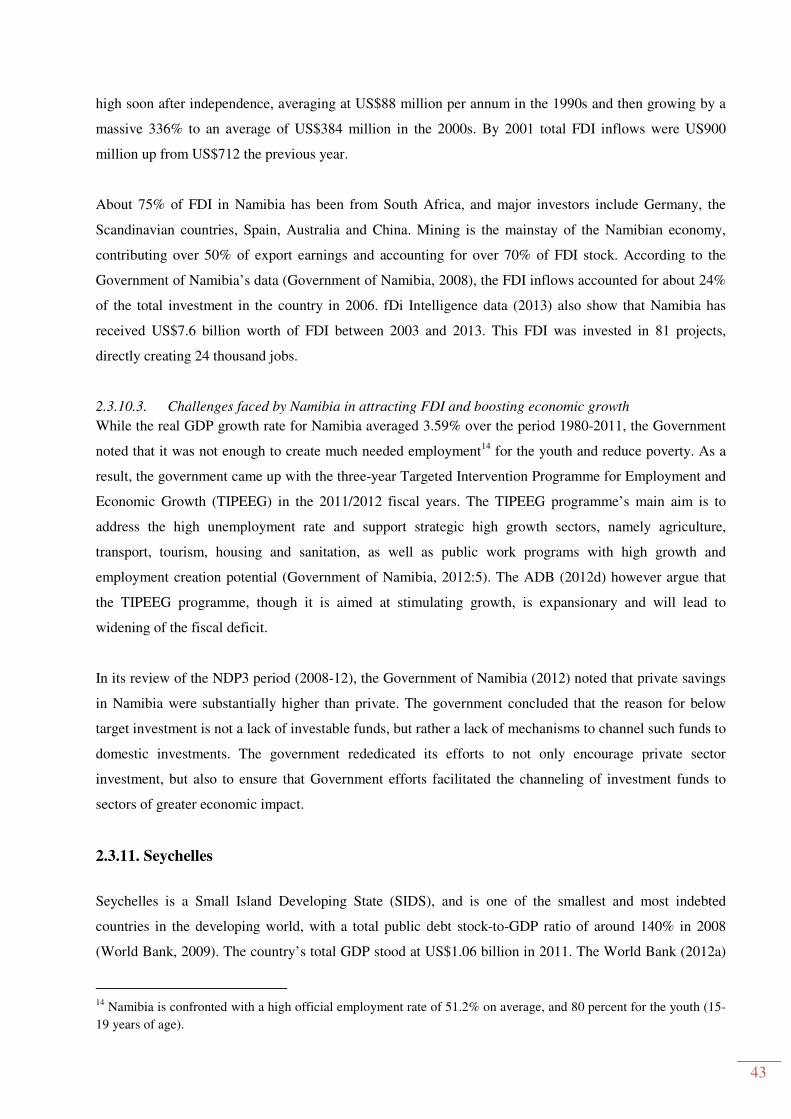
43
high soon after independence, averaging at US$88 million per annum in the 1990s and then growing by a
massive 336% to an average of US$384 million in the 2000s. By 2001 total FDI inflows were US900
million up from US$712 the previous year.
About 75% of FDI in Namibia has been from South Africa, and major investors include Germany, the
Scandinavian countries, Spain, Australia and China. Mining is the mainstay of the Namibian economy,
contributing over 50% of export earnings and accounting for over 70% of FDI stock. According to the
Government of Namibia’s data (Government of Namibia, 2008), the FDI inflows accounted for about 24%
of the total investment in the country in 2006. fDi Intelligence data (2013) also show that Namibia has
received US$7.6 billion worth of FDI between 2003 and 2013. This FDI was invested in 81 projects,
directly creating 24 thousand jobs.
2.3.10.3. Challenges faced by Namibia in attracting FDI and boosting economic growth
While the real GDP growth rate for Namibia averaged 3.59% over the period 1980-2011, the Government
noted that it was not enough to create much needed employment14 for the youth and reduce poverty. As a
result, the government came up with the three-year Targeted Intervention Programme for Employment and
Economic Growth (TIPEEG) in the 2011/2012 fiscal years. The TIPEEG programme’s main aim is to
address the high unemployment rate and support strategic high growth sectors, namely agriculture,
transport, tourism, housing and sanitation, as well as public work programs with high growth and
employment creation potential (Government of Namibia, 2012:5). The ADB (2012d) however argue that
the TIPEEG programme, though it is aimed at stimulating growth, is expansionary and will lead to
widening of the fiscal deficit.
In its review of the NDP3 period (2008-12), the Government of Namibia (2012) noted that private savings
in Namibia were substantially higher than private. The government concluded that the reason for below
target investment is not a lack of investable funds, but rather a lack of mechanisms to channel such funds to
domestic investments. The government rededicated its efforts to not only encourage private sector
investment, but also to ensure that Government efforts facilitated the channeling of investment funds to
sectors of greater economic impact.
2.3.11. Seychelles
Seychelles is a Small Island Developing State (SIDS), and is one of the smallest and most indebted
countries in the developing world, with a total public debt stock-to-GDP ratio of around 140% in 2008
(World Bank, 2009). The country’s total GDP stood at US$1.06 billion in 2011. The World Bank (2012a)
14 Namibia is confronted with a high official employment rate of 51.2% on average, and 80 percent for the youth (15-
19 years of age).

44
classified Seychelles as an upper-middle class country; its GDP per capita rose by more than four times –
from a mere US$2,288 in 1980 to US$12,321 in 2011. As a SIDS, the country’s economy faces constraints
characteristic of a small island state, such as lack of economic diversification, susceptibility to external
shocks, distance from markets, and risks of environmental degradation, and weather-related disasters
(World Bank, 2013i).
2.3.11.1. Policies to attract FDI and boost economic growth in Seychelles
The Government of Seychelles currently has an ambitious plan to double its GDP by the year 2017. This
objective is articulated in a development plan; Seychelles Strategy 2017-Creating our nation’s wealth
together (Government of Seychelles, 2007). The ADB (2011b) noted that before the country’s current
reform programme, the economy used to be managed under the state-led development strategy that
modeled on self-sufficiency and direct intervention in manufacturing, distribution, trade and other
economic activities through state owned enterprises (SOEs). These earlier policies were characterised by
persistent expansionary fiscal and monetary policies and incompatible trade and exchange rate policies,
which led to severe macroeconomic imbalances. In fact, the economy became so unstable that it failed to
honour its foreign debt obligations by 2008 (ADB, 2011b).
As part of the reform process, the Government has also been implementing Macro-Economic Reform
Programmes (MERPs). The first MERP was adopted in 2002 and was intended to assist in re-structuring
the country’s economy, and exploring ways to promote growth and raising the standard of living of the
citizenry. The first MERP also recognised the significance of the private sector in growing the economy
and creating employment for the youth. Through the MERP of 2002, the Government privatised many of
its assets (Government of Seychelles, 2010).
The second MERP started to be implemented in 2008. This was initiated with the support of major
development partners (including the ADB, WB, IMF and the European Union). The reforms undertaken
since 2008 include exchange rate and monetary policy deregulation, tax reform, elimination of subsidies,
and enactment of legislation such as the Public Debt Management Act. ADB (2011b) applauds these
reforms and attributes them to a major economic turnaround. By September 2011, Seychelles’ total public
debt ratio to GDP declined to 84% from 128% in 2008.
UNCTAD (2010) argues that SIDSs are by nature attractive destinations for FDI in tourism, as well as eco-
tourism. Seychelles has been taking advantage of its SIDS status by pursuing niche strategy, highlighting
tourism services with a combination of quality and exclusivity based on their small size – an offering not
always available in mass-market package destinations. Apart from attracting tourism related FDI, the
country has also marketed the Exclusive Economic Zone (EEZ) with the aim of directing FDI to offshore
oil exploration and other sectors in the bid to diversify the economy.

45
2.3.11.2. GDP and FDI trends in Seychelles
As shown in Figure 18, the country entered the 1980s in a recession, with the lowest real GDP growth of -
6.64% in 1981. The country however managed to bounce back and grew by 8% and 10% in 1984 and 1985
respectively. The economy slowed down in the late 1980s and early 1990s before peaking to a historic high
of 15% in 1997. The economy has been struggling in the 2000s, recording negative growth rates in half of
the ten years. The growth rate in 2011 was 5.11% down from 9.55% in the previous year.
Figure 18: GDP and FDI Trends in Seychelles (1980-2011)
Source: UNCTAD (2013a) Database
As illustrated above, FDI has been one of the major drivers of the Seychelles’ economy. The ADB (2012a)
argued that FDI has only been second to tourism in terms of driving the growth of the economy. Although
in values terms, FDI inflows are lower than other SADC countries, its ratio to GDP is higher, averaging
5% in the 1980s and 1990s and then more than doubled to average at 12% during the 2000s. In 2006 the
total FDI to GDP rose to a massive 23.4% before decreasing sharply to 1.4% in 2011. The country
recorded its highest level of FDI inflows in 2007, peaking at US$239 million before decreasing to US$143
million currently. The ADB (2012a) attributes increase in FDI in the later 2000s to the investments in the
completion of several high-end hotels, largely financed by foreign investors, and the construction of a
residential project in Ile Perseverance in 2009.
The Central Bank of Seychelles (2012) estimated that FDI inflows in 2012 amounted to US$117 million, a
reduction of US$28 million (20%) compared to 2011. The majority of these investments are directed
towards the tourism industry. The Central Bank also attributes the fall in FDI to completion of tourism or
hotel related projects. Major investing countries in the tourism sector are the United Kingdom, South
Africa, Belgium and India.
-10.00
-5.00
0.00
5.00
10.00
15.00
20.00
25.00
0
50
100
150
200
250
300
GD
P,
FDI
(%)
FDI
(US
$,
Mil
lio
ns)
FDI (US$, mln) GDP growth FDI (% of GDP)

46
fDi Intelligence data (2013) also showed that the Seychelles received US$2.2 billion worth of FDI between
2003 and 2013. This FDI was invested in 16 projects, directly creating 4,553 jobs.
2.3.11.3. Challenges faced by Seychelles in attracting FDI and boosting economic growth
As highlighted above, the country’s growth prospects had been hampered by expansionary economic
policies, which led to a debt overhang. This is however being addressed through the Government’s
partnership with development financial institutions such as ADB, WB and IMF. The Central Bank of
Seychelles (2012) attributes the reduction in FDI inflows over the years to the country’s vulnerability to
external shocks, uncertainties in developed economies and less available land area15 for investments. Both
ADB (2012a) and Central Bank of Seychelles (2012) make projections that FDI inflows will decelerate
from 2011 and in the near future, due to the completion of the large construction projects.
2.3.12. South Africa
South Africa’s total GDP was estimated at US$408 billion by the World Bank (2013j). The World Bank
(2013c) commends the democratic government16 for its persistent record of macro-economic shrewdness,
sound budgetary policies, and an ability to tap into a helpful global environment, which has enabled the
country’s GDP to grow at a steady pace for almost two decades up to the global financial crisis of 2008-
2009 (World Bank, 2013j). The country is currently ranked as an upper-middle income economy with GDP
per capita of US$8,070, up from US$3,547 in 1994 when the new democratic government was sworn in.
2.3.12.1. Policies to attract FDI and boost economic growth in South Africa
Soon after the ushering in of the democratic elections in 1994, the new government came up with the
Reconstruction and Development Programme (RDP), a socio economic development programme
advocating for greater equity as the basis for long-term development and growth (Government of South
Africa, 2011). The RDP encompassed interventions aimed at stimulating the economy such as checks on
fiscal spending, reduction of government borrowing, tax reduction, trade liberalisation, but with special
focus on social service extension to historically disadvantaged individuals, and roll-out of infrastructure
programmes (UN, 2011:6).
A macroeconomic policy framework called the Growth, Employment and Redistribution (GEAR) in the
year 1996 replaced the RDP. GEAR was aimed at achieving sustained annual real GDP growth of 6% or
more by the year 2000 while creating 400,000 new jobs each year (UN, 2011:6). This was supposed to be
achieved through (i) macroeconomic stabilisation and (ii) trade and financial liberalisation as a panacea to
fostering economic growth, increase employment and reducing poverty (Ncube, Shimeles and Verdier-
Chouchane, 2012:9). However UN (2011:7) argues that GEAR brought mixed outcomes. On one hand it is
15 As noted above, Seychelles is a Small Island Developing State (SIDS), and therefore has a very small land area. 16 This democratic government came into power through the first multiracial elections in 1994.

47
acclaimed for bringing in sound financial discipline and macroeconomic stability, while on the other is
blamed for failing to increase formal employment and more evenly distributed wealth (Gelb, 2003), not
meeting the GDP growth targets and failure to attract FDI as has been anticipated. Because of these
shortcomings, the government came up with a new macroeconomic policy in 2006; the Accelerated and
Shared Growth Initiative for South Africa (AsgiSA). As the name suggests, the AsgiSA was meant to help
the country in accelerating its growth and to ensure rising living standards for the majority (Government
of South Africa, 2006).
The current New Growth Path (NGP) and National Development Plan (NDP) replaced AsgiSA. The NGP
identifies various structural impediments to faster growth and makes recommendations on promoting
economic growth with employment creation. The NGP aims to create 5 million jobs by 2020 by identifying
sectors that present employment growth opportunities (referred to as ‘job drivers’) and grow the economy
at a rate of between 4% and 7% a year (Government of South Africa, 2010). The NDP on the other hand
encompasses NGP as it is a longer-term strategy up to 203017. The two policy documents tend to be
complementary as they both advocate for faster economic growth and increased employment creation
through mostly government interventions in the following ways: infrastructure investment, microeconomic
reforms that lower the costs of business, competitive and equitable wage structures, and the effective
unblocking of constraints to investment in certain sectors of the economy (Government of South Africa,
2011).
Though South Africa does not have a specific investment policy nor any specific incentives targeted at FDI
(Gelb and Black, 2004), the country has been using both its macro and micro economic policies and
strategies to attract foreign investment. Since 1996 the country has been restructuring its economy allowing
for more private sector participation, which includes the privatisation of state owned enterprises (SOEs)
Furthermore, recent policies like GEAR emphasised economic growth as a tool to stimulate FDI inflows,
while NGP sights FDI as one of the most important sources for funding the country’s developmental
initiatives, especially the green economy (Government of South Africa, 2010).
2.3.12.2. GDP and FDI trends in South Africa
The structure of the South Africa’s economy has been shifting from the primary (and resource dependent)
and secondary based economy to a tertiary and knowledge based economy. During the early 1980s, the
biggest sector in gross value added at basic was manufacturing followed by community, social and
personal services. The finance sector was the fourth largest sector in 1980 but has grown tremendously to
be the biggest sector by output in 2012; a 240% growth. The real output of agriculture, forestry and fishing
has been decreasing over the years, while the tertiary sector has been driving economic growth. See 2013
structure of South African economy in Figure 19.
17 Its full name is the National Development Plan: Vision 2030.

48
Figure 19: Structure of the South African Economy
Source: South Africa Reserve Bank (2013)
A closer analysis of the South African FDI levels and percentage of FDI to GDP over the 1980-2011
period shows that the new government inherited an economy which had very low FDI (averaging at less
than 0.05% of GDP per annum) and a shrinking economy (which had just decreased by a cumulative
3.47% during the 1990-1992). This was mainly because of the domestic unrest and sanctions imposed on
the apartheid government (Asafa-Adjei, 2007:100).
Smit and du Plessis (2006) attribute the low growth rates during the ten-year period from 1984 to 1993 to
the trade and financial sanctions and domestic political opposition to the then apartheid government. From
1994 to the global financial crisis in 2008, South Africa’s GDP had been growing an average of 3.6% per
annum. The economy took a knock in 2009 but quickly bounced back to 2.84% in 2009, 3.12% in 2011
and is estimated to have eased 2.5% in 2012 (Statistics South Africa, 2013).
As can be seen in Figure 20, South Africa suffered a net capital outflow in 1985, one year before
imposition of economic sanctions. Annual FDI inflows to South Africa averaged at 0.03 percent of GDP
from 1980 up to the democratic elections in 1994. Thereafter, FDI started to gradually increase, peaking at
5.7% of GDP in 2001, and averaging at 1.5% in the post-apartheid period.
Finance &
Insurance
21%
Community
18%
Manufacturing
15%
Government
13%
Wholesal
e &
Retail
12%
Transport
9%
Agriculture
5%
Construction
3%
Mining
2%
Electricity
2%
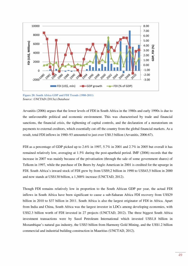
49
Figure 20: South Africa GDP and FDI Trends (1980-2011) Source: UNCTAD (2013a) Database
Arvanitis (2006) argues that the lower levels of FDI in South Africa in the 1980s and early 1990s is due to
the unfavourable political and economic environment. This was characterised by trade and financial
sanctions, the financial crisis, the tightening of capital controls, and the declaration of a moratorium on
payments to external creditors, which essentially cut off the country from the global financial markets. As a
result, total FDI inflows in 1980–93 amounted to just over U$0.3 billion (Arvanitis, 2006:67).
FDI as a percentage of GDP picked up to 2.6% in 1997, 5.7% in 2001 and 2.7% in 2005 but overall it has
remained relatively low, averaging at 1.5% during the post-apartheid period. IMF (2006) records that the
increase in 2007 was mainly because of the privatisation (through the sale of some government shares) of
Telkom in 1997, while the purchase of De Beers by Anglo American in 2001 is credited for the upsurge in
FDI. South Africa’s inward stock of FDI grew by from US$9,2 billion in 1990 to US$43,5 billion in 2000
and now stands at US$130 billion, a 1,300% increase (UNCTAD, 2012).
Though FDI remains relatively low in proportion to the South African GDP per year, the actual FDI
inflows in South Africa have been significant to cause a sub-Saharan Africa FDI recovery from US$29
billion in 2010 to $37 billion in 2011. South Africa is also the largest originator of FDI in Africa. Apart
from India and China, South Africa was the largest investor in LDCs among developing economies, with
US$2.3 billion worth of FDI invested in 27 projects (UNCTAD, 2012). The three biggest South Africa
investment transactions were by Sasol Petroleum International which invested US$1,8 billion in
Mozambique’s natural gas industry, the US$3 billion from Harmony Gold Mining, and the US$1.2 billion
commercial and industrial building construction in Mauritius (UNCTAD, 2012).
-3.00
-2.00
-1.00
0.00
1.00
2.00
3.00
4.00
5.00
6.00
7.00
8.00
-2000
0
2000
4000
6000
8000
10000
GD
P,
FDI
(%)
FDI
(US
$,
Mil
lio
ns)
FDI (US$, mln) GDP growth FDI (% of GDP)

50
Historically, the major sources of South African FDI are the United Kingdom, USA, Germany,
Netherlands and other European countries (Arvanitis, 2005:68), but there is a current shift to the BRICS18
countries. South Africa joined a bloc of emerging countries, BRICS, in December 2010. According to
UNCTAD (2013b), BRICS have emerged as major recipients of FDI and important outward investors, as
shown below:
• FDI inflows to BRICS more than tripled to an estimated US$263 billion in 2012 over the past
decade. Consequently, their share in world FDI flows rose to 20% in 2012, up from only 6% in
2000.
• BRICS’ outward FDI has risen from US$7 billion in 2000 to US$126 billion in 2012, or 9% of
world flows, from only 1% in 2000.
• In 2011 India invested US$194 million in South Africa’s automotive and ferrochrome
manufacturing plants through the Tata Group.
• One-fifth of the outward FDI stock of South Africa was located in the “BRIC” in 2011, mainly in
China. This outward FDI is mainly concentrated in mining, infrastructure and construction, and
finance and business services sectors.
• By 2011, four of the BRICS countries; South Africa, China, India and Russia – had risen to rank
among the top investing countries in Africa on FDI stock and flows.
As a member of BRICS, South Africa is expected to benefit from the formation of the BRICS bank, which
is anticipated to inject financial resources into infrastructure development.19 This comes against the
background of South Africa’s FDI inflows rising from US$1.23 billion in 2010 to US$5.81 billion in 2011,
where it is the second largest destination of FDI in Africa20. According to UNTAD (2012), South Africa
ranks 14th out of 21 countries rated by international companies (TNCs) as top prospective investment
destinations for 2012-2014. South Africa is seen as a highly competitive FDI destination in terms of natural
resources and infrastructure relative to its peers (Government of South Africa, 2013:198).
2.3.12.3. Challenges faced by South Africa in attracting FDI and boosting economic growth
As part of preparatory work for the National Development Plan: Vision for 2030, the South African
Government produced a Diagnostic Report which identified nine challenges to the socio economic
development of the country. The economic challenges identified include; skills shortage and lower quality
of education; poorly located, underdeveloped and insufficient infrastructure to foster higher growth; lack of
diversification where the economy is too resource dependent; and widespread corruption (Government of
18 BRICS (Brazil, Russia, India, China, South Africa) 19 According to outcomes of the Fifth BRICS Summit, the BRICS Leaders agreed to the establishment of a New
Development Bank and indicated that the initial capital contribution to the bank should be substantial and sufficient
for the bank to be effective in financing infrastructure. Available at: http://www.brics5.co.za/ (Accessed 21 May
2013) 20 SA is currently led in FDI inflows by Nigeria which received US$8.92 billion in 2011.

51
South Africa, 2011). Nevertheless, the country was ranked 52nd in in the world in The Global
Competitiveness Report (2012-13), making it the highest ranked country in SADC and 3rd among BRICs
economies. However the same report recommends that South Africa needs to work on the following to
improve its competitiveness: labor market inefficiency, skills shortage, poor security (which leads to a high
crime rate), high business costs and health of the workforce21.
2.3.13. Swaziland
The Kingdom of Swaziland (thereafter Swaziland) is a geographically small landlocked country with a
small open economy heavily reliant on export-based agricultural commodities and industries, especially
sugar exports and tourism and with more than 80% of its imports originating from South Africa
(Basdevant, Baba and Mircheva, 2011). Consequently, the country’s economic growth and development
are affected by climatic conditions, global economic developments and commodity prices, as well as
investments and aid flows. The country is classified as a medium-development country by the United
Nations (UN) and as a lower middle-income country by the World Bank (2012a).
2.3.13.1. Policies to attract FDI and boost economic growth in Swaziland
From its independence in 1968, the country’s socio economic development polies, strategies and goals
were set in successive five-year national development plans (NDPs) and in successive three-year rolling
development plans. However, in 1988, Government decided to embark on an improved and more
comprehensive planning system, and formulated the National Development Strategy (NDS). The NDS is a
national macroeconomic development policy, which set out a 25-year development framework from 1997
to 2022. The NDS states its vision as "By the Year 2022, the Kingdom of Swaziland will be in the top 10%
of the medium human development group of countries founded on sustainable economic development,
social justice and political stability" (Government of Swaziland, 1999).
Swaziland’s NDPs, on the other hand, are annual 3 year rolling plans, which depict policies, programmes
and projects per prioritised economic sector in terms of current and expected contribution to the economy.
Special priority is given to the “Millennium Projects”, which are aimed at accelerating investment in
infrastructure and tourism in order to create employment and reduce poverty (Government of Swaziland
and European Commission, 2002).
The country also has Economic and Social Reform Agenda (ESRA), which is a monitoring tool that
imposes pressure on ministries to perform efficiently and to accelerate implementation of programmes.
ESRAs are designed in phases, just like NDPs and are aimed at increasing the speed of economic growth,
and improving social services and administrative governance. Strategies to accelerate economic growth
21 Which has been affected by HIV and AIDS.

52
included promotion of large-scale investment, development of the small, medium and micro enterprise
sector and the development of a vibrant tourism sector (Government of Swaziland and European
Commission, 2002).
Other policies include the Millennium Action Programme (MAP), Smart Programme for Economic
Development (SPEED), Government's Programme of Action 2008-2013, Small and Medium Enterprises
Policy of 2005, Privatisation Policy, 2004 and the Decentralisation Policy, 2006.
The agency that is responsible for initiating, coordinating and facilitating the implementation of
government policies and strategies on investment is the Swaziland Investment Promotion Authority
(SIPA). SIPA was created through an Act of Parliament in 1998 (SIPA, 2012), and the same Act sets out
general principles in regard to investor treatment and deals with protection of investment and settlement of
investment disputes.
In the Swaziland Investment Policy of 2009, the government “notes the importance of political stability to
inflows of foreign direct and portfolio investment as well as locally-generated investment” (USAID,
2009:15). The goals of the investment policy, among other things are to: (i) increase levels of investment,
which will increase economic growth, (ii) increased employment opportunities, (iii) encourage higher
levels of productivity in the economy, (iv) export development, (v) increase levels of management skills,
(vi) promotion of new technology and (vii) encouraging the growth of small enterprises.
The policy allows all types of private investment (except that which contravenes the Swazi legislation) and
offers incentives to domestic investors with a minimum of US$50,000 and foreign investors with
US$100,000 minimum investment.
2.3.13.2. GDP and FDI trends in Swaziland
The country experienced rapid economic growth during the 1980s, averaging at 6.88% per annum and
peaking at 14.63% in 1987. The Government of Swaziland and European Commission (2002) attributed
this growth to an increase in foreign investment. Foreign investment, during this period was mainly driven
by dis-investment from South Africa (owing to sanctions and apartheid related challenges) and the
country’s perceived investor benefits such as access to larger southern African markets; preferential access
to Europe and North America; availability of sugar and timber at competitive prices; a fairly stable
economy and a country supportive of the private sector. However the GDP growth rates decreased to an
average of 3.66% in the 1990s, and worsened to 2.29% in the 2000s. In 2011, the country recorded one of
the lowest growth rates in SADC (0.25%), and the ADB (2012a) attributes the decline to contraction in the
manufacturing sector. It notes that the textile sub-sector was struck by the global economic crisis of 2009,
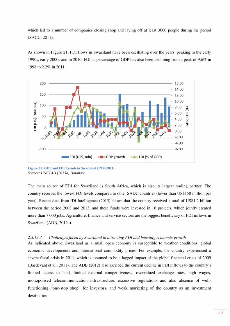
53
which led to a number of companies closing shop and laying off at least 3000 people during the period
(SACU, 2011).
As shown in Figure 21, FDI flows in Swaziland have been oscillating over the years, peaking in the early
1990s, early 2000s and in 2010. FDI as percentage of GDP has also been declining from a peak of 9.6% in
1998 to 2.2% in 2011.
Figure 21: GDP and FDI Trends in Swaziland (1980-2011)
Source: UNCTAD (2013a) Database
The main source of FDI for Swaziland is South Africa, which is also its largest trading partner. The
country receives the lowest FDI levels compared to other SADC countries (lower than US$150 million per
year). Recent data from fDi Intelligence (2013) shows that the country received a total of US$1.2 billion
between the period 2003 and 2013, and these funds were invested in 16 projects, which jointly created
more than 7 000 jobs. Agriculture, finance and service sectors are the biggest beneficiary of FDI inflows in
Swaziland (ADB, 2012a).
2.3.13.3. Challenges faced by Swaziland in attracting FDI and boosting economic growth
As indicated above, Swaziland as a small open economy is susceptible to weather conditions, global
economic developments and international commodity prices. For example, the country experienced a
severe fiscal crisis in 2011, which is assumed to be a lagged impact of the global financial crisis of 2009
(Basdevant et al., 2011). The ADB (2012) also ascribed the current decline in FDI inflows to the country’s
limited access to land, limited external competitiveness, overvalued exchange rates, high wages,
monopolised telecommunication infrastructure, excessive regulations and also absence of well-
functioning “one-stop shop” for investors, and weak marketing of the country as an investment
destination.
-6.00
-4.00
-2.00
0.00
2.00
4.00
6.00
8.00
10.00
12.00
14.00
16.00
-100
-50
0
50
100
150
200
GD
P,
FDI
(%)
FDI
(US
$,
Mil
lio
ns)
FDI (US$, mln) GDP growth FDI (% of GDP)

54
2.3.14. Tanzania
The United Republic of Tanzania (here referred to as Tanzania) is classified as a low- income country with
a total GDP (at current prices) of US$23.87 billion by 2011. Its GDP per capita was US$532 in 2011, up
from US$308 in 2000, and only US$172 in 1990. Tanzania was among the first countries to benefit by
reaching the HIPC completion point on November 27, 2001. According to the World Bank (2013k), the
country’s economy is agro-based, with agriculture contributing more than 40% to GDP. The sector also
employs 80% of the working population, and accounts for 64% of all exports. The country is regarded as
one of Africa’s ‘success stories’, with GDP growth averaging 3.5% in the 1990s and around 7% in the
2000s.
2.3.14.1. Policies to attract FDI and boost economic growth in Tanzania
Tanzania’s macroeconomic history is chronicled in Nord, et al. (2009) and Robinson, Gaertner and
Papageoriou (2011). The country transited from socialism’s command economy soon after independence in
the 1960s to market-oriented developing economy since the 1980s. The three phases of Tanzania’s
economic transformation are summarised below:
i. Ujamaa Socialism and Economic Decline (1967–1985): The economy was characterised by state
control and ownership and command system, where state owned enterprises drove the economy.
This resulted in economic decline, shortage of goods, high inflation, and decrease in exports
among other economic ills.
ii. Liberalisation and Partial Reforms (1986–1995): This was the first phase of recovery and reform.
It included the gradually liberalisation of the economy as envisioned under the Economic Recovery
Programme (ERP) of 1986. Under the ERP, a market economic system was introduced through
prices adjustments, deregulation of exchange rates, and removal of controls on economic activities
by way of privatisation. However, the economy did not grow nor stabilise as envisaged.
iii. Macroeconomic Stabilisation and Structural Reforms (1996–): Further reforms included unifying
the exchange rate, liberalisation of the financial sector, trade reforms and development of a market-
oriented regulatory framework. This resulted in higher economic growth rates (see graph below)
and stabilisation of the economy.
The country recently adopted a development framework, and long-term social and economic development
goals based on a National Vision 2025 and Zanzibar Vision 2020 (Government of Tanzania, 2003). Its
short to medium term development framework includes the National Poverty Eradication Strategy (NPES),
which guides the country’s development and poverty strategies; the National Strategy for Growth and
55
Reduction of Poverty (NSGRP)22; and the Zanzibar adopted a Strategy for Growth and Reduction of
Poverty (ZSGRP)23.
According to the Bank of Tanzania (2012), the current policies, both monetary and fiscal, are aimed at
sustaining macroeconomic stability. Nord et al. (2009) highlight that Tanzania, during its second
economic-reform phase, began to implement measures to attract FDI. The country enacted an Investment
Promotion Policy in 1990; and it reviewed this in 1996 in an effort to broaden its improvement in the
investment climate of the country (UNCTAD, 2002a). Some of the earlier institutional and regulatory
reforms included the establishment of the Zanzibar Investment Promotion Agency (ZIPA) in 1986, and the
ensuing formation of the Free Economic Zones (FEZs), and the national Investment Promotion Centre
(IPC). These are all aimed at the facilitation and management of both domestic investment and FDI.
Some incentives and initiatives under this regime include the lowering and rationalisation of tariff rates,
and the liberalisation of foreign direct investments. The Government of Tanzania also adopted a National
Trade Policy in 2003, which advocated the further removal of regulatory and administrative constraints to
FDI inflows in the short term, and the expediting of reforms of the legal and regulatory framework, as well
as allowing self-regulation by the private sector, as part of long- term measures to create an enabling
business environment, and to increase FDI flows (UNCTAD, 2002a).
2.3.14.2. GDP and FDI trends in Tanzania
As briefly discussed above, Tanzania is regarded of one of Africa’s ‘success stories’, owing to its almost
three decades of positive economic growth. The country entered the 1980s in a recession, recording a
2.38% real GDP growth in 1983 but bounced to 3.38% in the following year (see Figure 22). The country’s
GDP growth averaging 2.36% in the 1980s, increased to 4.37%, and buoyed to 6.74% in the 2000s. It
dipped to 6.04% in 2009 from an impressive 7.38% the previous year, and thereafter it averaged at 6.83%
for the next two years. It is important to note that soon after the reforms of 1996 the growth picked to
average at more than 6% per annum.
22 or MKUKUTA in Swahili. 23 Referred to as MKUZA.

56
Figure 22: GDP and FDI Trends in Tanzania (1980-2011)
Source: UNCTAD (2013a) Database
FDI inflows also benefited from the economic reforms. Before 1996 the level of FDI per annum averaged a
paltry US$8.8 million. The increase started to be noticeable soon after the adoption of the Investment
Promotion Policy in 1992, and its review in 1996-97 coincided with even more inflows. In the late 1990s,
FDI inflows stabilised at around US$150 million and then grew to an average of US$355 million in the
early 2000s before a sharp acceleration to an average of US$824 million in the late 2000s. By 2011 total
FDI inflows stood at US$1.1 billion, which is more than 20 times higher than the pre-1995 reform period.
As a percentage of GDP, FDI grew from an average of 0.15% pre-reforms to a peak of 6.5% in 2005 before
decreasing to an average of 4.21%. According to Nord, et al. (2009), the country has been successful
compared to its peers in sub-Saharan Africa in attracting foreign investments.
The biggest beneficiary of FDI inflows is the mining sector, and recently in oil and gas explorations, and
major infrastructural electric power projects (UNCTAD, 2012). Other sectors such as the traditional
agriculture sector, tourism and manufacturing have also been receiving FDI. fDi Intelligence (2013) data
shows that the country received a total of US$15 billion worth of FDI in the period 2003 to 2013 and this
amount was invested in 159 projects, creating more than 31 thousand jobs.
2.3.14.3. Challenges faced by Tanzania in attracting FDI and boosting economic growth
The World Bank (2013k) noted that although the country’s economy has been high and relatively stable
over the past decades, its sources of growth are confined to a few sectors, and the growth was turning out
to be increasingly reliant on government spending, instead of on private investment. The World Bank
(2013e) further projected that the country could become a major producer of natural gas in a decade, which
could be a major attraction for FDI. However, the bank cautioned that an increase in FDI would only be
-4.00
-2.00
0.00
2.00
4.00
6.00
8.00
10.00
-200
0
200
400
600
800
1000
1200
1400
GD
P,
FDI
(%)
FDI
(US
$,
Mil
lio
ns)
FDI (US$, mln) GDP growth FDI (% of GDP)

57
possible if the country invested in its infrastructure and energy, and also undertook structural reforms,
especially aimed at improving the overall business environment.
In its Tanzania Policy Review Report, UNCTAD (2002a:1) recommended that Tanzania should replace its
1997 Investment Act – given the current environments, both inside and outside the country. The report also
suggested reviews of the country’s commercial and contract laws, labour laws, competition law, and the
updating of policies in sectors, such as fishing, mining and tourism.
2.3.15. Zambia
Zambia’s total real GDP stood at US$10.5 billion in 2011; and it is estimated to have grown to US$11.2
billion in 2012. The country’s economy has had over a decade of rapid growth, averaging at 4.75% per
annum between 1996 and 2011. The World Bank classified Zambia as a lower-middle income country in
July 2011 (World Bank 2013l), exactly seven years after reaching its HIPC completion point in 2005 (IMF,
2005). The country’s GDP per capita fell from US$673 in 1980 to US$319 in 2000; but it has since
rebounded to reach US$1,425 in 2011.
2.3.15.1. Policies to attract FDI and boost economic growth in Zambia
Thurlow and Wobst (2004) argue that Zambia’s economic development history has been shaped by the
expansion and eventual decline of the mining sector (especially copper) and the resultant economic
structural adjustment, which began in 1991. These economic development phases are summarised in Table
2 below, as chronicled by Saasa (1996); Thurlow and Wobst (2004); and the Government of Zambia
(2004).

58
Table 2: Phases of Economic Development Trajectory in Zambia
Economic policy Period Policy Actions and Result
Pre-policy reforms 1964-1983 − Centrally planned and protectionism, with heavy state control in the
ownership and management of economic activities.
− Economic policies were focused on import substitution, protection of
domestic industry from external competition and government directives on
investments, through industrial licensing,
− The economy was heavily dependent on copper and the proceeds of which
were used to subsidise agricultural produce
− As a result, the economy deteriorated, mainly as a result of the oil price
shock, the falling copper prices in the 1970s, and inadequate economic-
management responses.
Economic Structural
Adjustment
Programme
1983-87 − Deregulation and privatisation of the economy.
− However, the partial removal of exchange controls led to a substantial
depreciation of the local currency (kwacha), and an increase in inflation.
This led to food riots in 1986, threatened mining revenues, and
undermined political support.
Policy reversal 1987-89 − Fearing a loss in political power, the government abandoned the recently
introduced market-based reforms and reverted back to a command-style
economy, which included exchange rate controls, fixing of interest rates,
price controls on designated products.
− This led to shortages in the market, and the government responded by
introducing food coupons to lessen the burden of subsidies and to ration
the commodities.
Liberalisation 1990-91 − Reintroduction of economic liberalisation through relaxing exchange and
trade controls, privatisation and public sector reform.
− This was, however, accompanied by fiscal and monetary policy
contraction.
− This did not work, and then government lost the elections.
Economic reforms 1991- − Economic restructuring programme under the direction and support of the
International Financial Institutions (IFIs) and bilateral donors.
− The policies included macro-economic stabilisation, public sector reform,
external liberalisation, market-based agricultural reforms, and the
privatisation of state assets.
− The result was a new growth path, which includes sustained decrease in
inflation (to less than 10% currently), growth in the economy averaging at
more than 5% in the 2000s, and FDI averaging more than 7% of GDP per
annum in the same period.
Source: Own illustration from Saasa (1996), Thurlow and Wobst (2004) and Government of Zambia
(2004)

59
From 1991 to date, Zambia has been producing policies and strategies aimed at boosting economic growth
and attracting FDI. These include the National Action Plan; the Public Investment Programmes of 2000-
2002 and 2001-2003; the Zambia Poverty Reduction Strategy Paper 2002-2004; the Five-year Institutional
Strategic Plans; the Sectoral Investment Programmes; and the three-year rolling Medium-Term
Expenditure Framework (MTEF) (Mwanawina, 2007).
In a bid to stimulate both domestic and foreign investment, the Government of Zambia adopted an
Investment Code in 1994. The code was amended and incorporated into the Zambian Development Agency
Act of 2006, which gave birth to the Zambia Development Agency (ZDA). The mandate of ZDA is to
address the private sector development needs of the country (UNCTAD, 2011a). In 2004, the Government
launched the Private Sector Development-Reform Programme (PSDRP), aimed at improving the
investment climate, reducing the cost of doing business and stimulating rapid and sustained private sector-
led economic growth (OECD, 2011). The country also set up special economic zones, through the support
of the Chinese, to incentivise both foreign and domestic investors (Alves, 2012).
Zambia has also been undertaking reforms that are aimed at making it easier for enterprises to do business.
These efforts have resulted in Zambia’s improved ranking on the World Bank‘s Doing-Business Index,
moving from 90 in 2009 to 76 in 2010 out of 183 economies. Additionally, Zambia has attained a
sovereign credit rating of “B+ with a stable outlook” by Fitch Ratings in March 2011. Furthermore,
Zambia is seen as one of the most open economies to foreign equity ownership (OECD, 2011).
2.3.15.2. GDP and FDI trends in Zambia
During the period under review (1980-2011), the economy of Zambia passed through a turbulent period in
the late 1980s to early 1990s (see Figure 23). Real GDP fell by a massive 8.6% while FDI as a percentage
of GDP fell to a paltry 1.2% in 1994 and inflation peaked at above 180% per annum in 1993. However the
economic reforms started bearing fruit in the late 1990s. Zambia has grown faster than most of its peers24
and its growth has been broad-based, led by agriculture, manufacturing, services, and mining (World Bank,
2012b:3). The economy fell from an average annual real growth rate of 1.44% in the 1980s to 0.37% in the
1990s before taking off to 5.21% in the 2000s. It has now gone for over a decade, recording positive
growth from 1999. By 2011 grew by 6.6%, down from 7.11% the previous year as shown in the figure
below. The World Bank (2013L) attributes the recent buoyant growth to a mixture of shrewd macro-
economic management, market liberalisation and privatisation, investments in the copper industry (which
is the mainstay of the economy) and related infrastructure, and steep increase in copper prices.
24 Both mineral-producing and non-mineral-producing Southern African countries.

60
Figure 23: GDP and FDI Trends in Zambia (1980-2011) Source: UNCTAD (2013a) Database
As illustrated on the figure above, FDI inflows into Zambia follow the reform trajectory of the country.
The pre-reform period (before 1983) had very little inflows, and recorded a US$38 million net outflow in
1982. The fluctuations in FDI inflows in the late 1980s and the greater part of 1990s can be attributed to
the ‘stop-go’ implementation of the SAP by the Zambian Government (Saasa, 1996). Data from the
UNCTAD’s 2012 World Investment Report shows that FDI inflows into Zambia rose from approximately
US$164.9 million in 2003 to US$1.73 billion in 2010 and US$2 billion in 2011. FDI inflows continue to be
directed mainly at the mining sector, with manufacturing, communications, and financial institutions also
contributing to recent FDI growth. World Bank (2012b) forecasts that FDI inflows in Zambia will
continue, mainly towards copper mining, whose international prices are estimated to rebound from
US$7,900 per metric ton in 2012 to US$8,500 in 2013 before declining back to US$8,000 in 2014. The
short to medium term projects in the mining sector include the expansion of existing mines; Kansanshi,
Lumwana, and Konkola and the construction of new mines such as the First Quantum Trident mine and
smelter project (World Bank, 2012b:7).
While the mining sector remains the main attraction for the bulk of domestic and foreign investment, the
services sector, especially banking and tourism, and agriculture, have also attracted significant volumes of
FDI. fDi Intelligence (2003) shows that Zambia received a total of US$14.6 billion worth of FDI between
2003 and 2013, and this amount was invested in 137 projects resulting in 47 696 new jobs.
2.3.15.3. Challenges faced by Zambia in attracting FDI and boosting economic growth
In its Economic Brief on Zambia, the World Bank (2012b) acknowledges that medium-term prospects for
the country’s economic growth continue to be strong, but cautioned against significant challenges
stemming from global uncertainties, as Zambia’s economy is heavily dependent on copper exports and fuel
-10.00
-5.00
0.00
5.00
10.00
15.00
-500
0
500
1000
1500
2000
2500
GD
P,
FDI
(%)
FDI
(US
$,
Mil
lio
ns)
FDI (US$, mln) GDP growth FDI (% of GDP)

61
imports. The Government of Zambia (2004) highlighted the following as some of the main challenges
faced by the Zambian economy: the lack of proper co-ordination of fiscal and monetary policy, leading to
persistent fiscal deficits; underdeveloped and segmented financial markets, which limit the country’s
ability to attract more FDI; and low savings and investments.
In its Zambian Investment Policy Review report, the OECD (2011) lauded Zambia for its efforts and
successes in improving the business and investment environment over the past years, but noted the lack of
“a complete and coherent investment policy”. The study also highlighted that ZDA’s current mandate was
too broad, considering its capacity, thus limiting its ability to promote and facilitate investment in a
focused manner. Other recommendations include the development of a predictable and fair tax system, and
the easing of bureaucratic and costly processing in obtaining incentives for investment.
2.3.16. Zimbabwe
The World Bank (2013m) estimated the country’s nominal GDP at US$10.8 billion in 2012 up from
US$9.9 billion in the previous year. The Word Bank data also shows that Zimbabwe’s GDP per capita
(current prices), which has been decreasing since its independence in 1980, has now started to increase. In
1980, Zimbabwe’s GDP per capita was US$916; but it fell to US$840 in 1990, and then further to US$535
in 2000; but it has now started to increase since the formation of the Government of National Unity (GNU)
in 2009; and it stood at US$723 by 2011. Zimbabwe is currently classified as a low-income country by the
World Bank (2012a). It is currently the only SADC country, which uses the United States of America
dollar as its official currency, after the introduction of a multicurrency regime25 into the economy in 2009
(Government of Zimbabwe, 2009).
2.3.16.1. Policies to attract FDI and boost economic growth in Zimbabwe
Like many SADC countries described above; the previous colonial regime, the liberation struggle,
socialism and the economic structural adjustment programme as advocated by the Bretton Woods
institutions, shape Zimbabwe’s macroeconomic policy history. These macroeconomic policy phases are
summarised below.
i. Import-substituting industrialisation and economic diversification (1965-1980): The settler regime
unilaterally declared its independence from British government in 1965. This led to international
isolation as the United Nations instituted sanctions in 1968. In response to the sanctions, the then
Rhodesian Government introduced import-substituting industrialisation and economic
diversification policies. As a result, the country’s GDP grew at an annual rate of above 7%
25 Apart from the US dollar, other currencies in circulation in Zimbabwe are the South African Rand and the
Botswana Pula.

62
between 1965 and 1974, but later the escalating war of liberation which led to independence in
1980, interrupted economic activity (Davies and Rattsø, 2000).
ii. Inward-looking policy (1980-1990): The new government adopted a socialist based economic
policy approach, whose goal was the usage of state intervention to redirect development for the
equitable benefit of the citizenry (Green and Khadani, 1986). The overall policy goal was ‘growth
and equity’ (Government of Zimbabwe, 1981). The import control policy from the sanctions era
was continued (Davies and Rattsø, 2000); government administratively allocated foreign exchange
to companies for both working capital and investment purposes. According to Gwenhamo
(2009:3), the government adopted a highly controlled and inward looking economy characterised
by market interventions and investment controls.
iii. Economic Structural Adjustment Programmes (ESAP)-1991-2000: under the guidance of the
Bretton Woods institutions, the Government of Zimbabwe adopted the ESAP policy in 1991. The
policy programme’s key focus area was economic and trade liberalisation (Davies & Rattsø, 2000),
which would in turn lead to increase in economic growth and surge of domestic and foreign
investment (Ndlela, 2011). Prescribed policy measures entailed reducing government expenditure,
commercialising and privatising some state owned enterprises, removal of market controls and
subsidies, and general economic liberalisation (Government of Zimbabwe, 1991). However, ESAP
did not yield much result on the economy as anticipated; an annual GDP growth rate of less than
1% was recorded (Government of Zimbabwe, 1996). This led the Government to embark on a new
policy, Zimbabwe Programme for Economic and Social Transformation (ZIMPREST), which was
taking on the experiences from the limitations and shortcomings of ESAP, and sought to re-
establish macro-economic stability, poverty alleviation as well as facilitating public and private
savings and investment (Zhou and Zvoushe, 2012).
iv. Economic crisis (2000-2008): The Government introduced economic empowerment and land
reform policies. Some of the programmes during this period include the Millennium Economic
Recovery Programme (MERP), which was launched in 2001, the National Economic Revival
Programme (NERP) of 2003, and the Macroeconomic Policy Framework (2005–2006) which was
aimed at rejuvenating the economy and building a sustained economic growth path. Despite all
these efforts, the period is characterised by socio-politico-economic meltdown whose peak year
was 2008 (Cousins, 2003). Some of the efforts were negated by the Government’s fast track land
reform programme, which led to the disruption of the agriculture sector (once the backbone of the
economy). This led an unmatched hyperinflationary environment, with the rate of 7 982% in
September 2007 (Government of Zimbabwe, 2009:3). There was also an acute shortage of basic
commodities which included maize meal (staple food), drugs, fuel, electricity and foreign currency
(Zhou and Zvoushe, 2012).
v. Economic recovery and stabilisation (2009-2012): Soon after the formation of the GNU in 2009,
the Government quickly introduced macroeconomic policies aimed at recovery and stability. It

63
adopted the Short Term Emergency Recovery Programme (STERP I & II), whose major
achievement was ‘macro-economic stability’ (Government of Zimbabwe, 2011) and further
launched the Medium Term Plan (MTP 2011-2015) whose main goal is to goal is “to transform the
economy, reduce poverty, create jobs, maintain macroeconomic stability and restore the
economy’s capacity to produce goods and services competitively” (Government of Zimbabwe,
2011:1).
The FDI and investment policies for Zimbabwe followed the same macroeconomic policies described
above. For example, at independence in 1980, the new Zimbabwean government adopted a highly
regulated and inward looking economy and continued with amply interventionist economic policies taken
over from the colonial government. Appraisals and approvals of foreign investment proposals involved an
overly long process, as the firms were obliged to get authorisation from the Foreign Investment Centre for
the development of any new enterprises in the country. As a result of these bureaucratic administrative
processes, FDI was very low in the 1980s (Gwenhamo, 2009).
The 1990s reforms, which included ESAP and ZIMPREST, were aimed at liberalising the economy and
attracting FDI. As part of this reform, the country established the Zimbabwe Investment Center (ZIC), a
‘one stop shop’ for investment approvals; offered enticements such as tariff and tax exemptions export
processing zones incentives in the form of tax holidays and customs free trade (Gwenhamo, 2009). This
was all part of the Government’s policy of structural adjustments, privatisation and liberalisation of the
economy.
In a bid to revive the economy and attract FDI after the economic crisis, the Government crafted many
policies, which include the Industrial Development Policy (IDP), and The National Trade Policy (NTP).
The NTP notes the reduction in the administration and processing of applications for investment licences
from 49 working days to 5 due to the establishment of ZIC and declares the openness of Zimbabwe to FDI.
It further highlights that the country is open to FDI directed into strategic sectors that include green-field
investment, export-oriented investments, promotion of Public-Private Partnerships (PPPs) and the services
sector, while barring foreign investments in retail merchandising (Government of Zimbabwe, 2011). The
country also adopted the Indigenisation and Economic Empowerment in 2007, which advocated for the
indigenisation of up to 51% of all foreign-owned businesses (UNCTAD, 2011b).
2.3.16.2. GDP and FDI trends in Zimbabwe
Figure 24 shows Zimbabwe’s GDP and FDI trends. The country’s GDP grew at an average of 1.42%% per
annum during the period 1970-1980, 3.32% during 1980-1989, 1.44% in 1990-2000 and -2.84% from 2000
to 2010. However, this per decade analysis masks the effects of the three drought-affected years (1992,
1993, and 1995), where real GDP growth averaged 2.6% and a low of -7% in 1992. The country was also

64
to endure a decade of negative growth between 1998 and 2008, during which the country experienced
hyperinflation where it required 24.7 hours only for prices to double (Hanke and Kwok, 2009:356). The
World Bank (2013m) estimated the cumulative decade long decline at 45% GDP contraction.
The economy of Zimbabwe quickly responded from the formation of the GNU in 2009 and the new
Government’s policies as GDP came from minus 4.74% 2008 to an impressive 7.21% in 2009. It further
increased to 9% in 2010 before slowing down to 6% in 2011.
Figure 24: Zimbabwe GDP and FDI Trends (1980-2011) Source: UNCTAD (2013a) Database
FDI inflows were very low in the 1980s, averaging at US$8 million per annum, constituting an average of
0.09% of GDP. FDI inflows increased substantially in the 1990s, due to the economic adjustment
programmes, which were in favour of economic liberalisation and attraction of foreign investors. The
country received its highest FDI inflows in a single year in 1998 when US$444 million was recorded.
Makola (2003) attributes this surge in investment to the then privatisation and liberalisation wave in the
economy, which attracted foreign capital mostly from South Africa, into various sectors of the economy.
During the Zimbabwean economic crisis of 2000-2008, FDI was US$37 million per year. However, the
establishment of the GNU (which brought some political stability and economic stability) saw the increase
of FDI net inflows of nearly eightfold in four years to US$387 million in 2011, up from just US$51.6
million in 2008. The major attraction for FDI in Zimbabwe has been mining, manufacturing, financial
services and banking. For example, UNCTAD (2012:69) recorded that the country received a US$4 billion
investment from the Essar Group (from India). This amount contributed to the bulk of the rise in
Zimbabwe’s greenfield investments from US$0.8 billion in 2010 to US$5.8 billion in 2011, making
Zimbabwe the biggest recipient among African LLDCs.
-10.00
-5.00
0.00
5.00
10.00
15.00
0
50
100
150
200
250
300
350
400
450
500
GD
P,
FDI
(%)
FDI
(US
$,
Mil
lio
ns)
FDI (US$, mln) GDP growth FDI (% of GDP)

65
Apart from India and China, South Africa and some European countries have been leading the foreign
investment in Zimbabwe in recent years. Data from fDi Intelligence (2013) shows that the country received
a total of US$13 billion during the period 2003 to 2013 and this amount was invested in 64 projects,
creating 24 418 direct jobs.
2.3.16.3. Challenges faced by Zimbabwe in attracting FDI and boosting economic growth
Although the country has shown signs of recovery since the formation of the GNU in 2009, the World
Bank (2013m) noted that the economy is still fragile, owing to political uncertainties, debt distress,
downside risks in agriculture, low domestic liquidity and high real-interest rates, high wages, the
dilapidated infrastructure, and an unreliable power supply (World Bank, 2013m). The IMF (2013)
recommends that the country should consider indigenisation and empowerment policies that provide
transparent rules, and offer due regard to property rights, which would help in building investor confidence
and in attracting the much-needed FDI.
2.4. Conclusion
Both SADC as a region and its member countries have been active over the last three decades in coming up
with policies, strategies and initiatives to boost economic growth and attract FDI. The major findings of
this chapter are that in the 1980s and early 1990s, most SADC countries were still coming out of
colonialism; and hence their policies were mainly focused on import substitution, socialism and command
economies, with strong emphasis on the protection of infant industries. In particular, the governments of
some of these countries were very active in the market through State-owned enterprises (SOEs), especially
in ‘strategic sectors’, such as telecommunication, agriculture and mining. Most of these policies had a
somewhat negative effect on FDI inflows. As a result, FDI inflows were fairly low during the first two
decades.
However, during the 1990s and the early 2000s, some of these countries developed strategies and policies
that were aimed at attracting FDI inflows. Some governments started embarking on privatisation,
liberalisation and economic structural-adjustment programmes. They also established government-funded
agencies, whose sole mandate was to attract and promote investment. These reforms saw the warming up
of countries to MNCs. Some of the policies that were implemented by these countries include: i) the
deregulation of the economy; ii) the relaxation of exchange controls; iii) the adoption of 'market-friendly'
policies, such as privatisation and trade liberalisation; iv) the protection of foreign investments; v) political
stability; and vi) participation in multilateral and bilateral trade and investment agreements.
Consequently, FDI inflows into some of these countries started picking up from the 1990s. In particular,
countries that pursued the privatisation of SOEs, such as Botswana, South Africa, Zambia, Angola,

66
Mozambique and Tanzania have attracted substantial amounts of FDI inflows during the last two decades;
and have seen their economies grow at a faster rate.
Moreover, in recent years, some of these countries have introduced special economic zones that offer
further incentives to investors in ‘strategic industries’, such as manufacturing, tourism and oil exploration.
However, overall, the FDI inflows into SADC countries can be described as resource seeking26, as the
greatest proportion of the funds are invested in the extractive sectors.
These policies and strategies adopted by SADC and its member countries in the last 3 decades had a
significant impact as FDI flowed into SADC. FDI inflows grew by almost fifty times, from US$372
million in 1980 to US$17 billion in 2008.
The main source countries for SADC destined FDI are the United States of America, United Kingdom,
India, Australia, and South Africa. Other SADC countries, which are investing in the region, are Mauritius,
Namibia and Zimbabwe. Overall, more than 80% of the FDI into SADC comes from the Americas, Europe
and Asia.
Notwithstanding a remarkable increase in FDI inflows in recent years in these countries, there are still a
number of challenges facing some of these countries. These include, inter alia, civil wars, social unrest and
political strife, which ravaged some of these economies during the 1990s and the early 2000s.
26 See definition section on the FDI in the next Chapter.

67
CHAPTER 3: THEORETICAL AND EMPIRICAL LITERATURE REVIEW
3.1. Introduction
This chapter reviews the theoretical link between FDI and economic growth and discusses previous studies
of the causal relationship between the two variables. The focus of the section is to document the
methodologies; sources and nature of data, findings and conclusions arrived at by other researchers. This
information will help, not only in the design of the model, but interpretation and comparisons of results
from this study.
The chapter is subdivided into two broad sections: a theoretical and empirical literature review. The
theoretical section investigates the economic link between FDI and economic growth. It starts by defining
FDI before exploring the channels through which FDI affects economic growth. The second section
presents seminal literature on the causal link between the two variables. The studies are organised in terms
of the type of data and methodology used; namely time series, cross-section and panel data respectively.
3.2. FDI and economic growth: Theoretical considerations
3.2.1. Definition of FDI
Krugman and Obstfeld (2008:163) defined FDI as “international capital flows in which a firm in one
country creates or expands a subsidiary in another” country. This involves the transfer of financial and
other resources and the gaining of control of another company in a host country. De Mello (1999:135)
defined FDI broadly as a type of “international inter-firm cooperation that involves significant equity stake
and effective management decision power in, or ownership control of, foreign enterprises”. This broad
definition encompasses the ability of FDI to transfer both tangible and intangible assets, which includes
flow of capital, research and development (R&D), management skills, production know-how (or expertise)
and better technology into the host country (De Mello, 1997; 1999; Balasubramanyam, Salisu and
Sapsford, 1999; Carbaugh, 2008).
The IMF and UNCTAD give the accounting and policy definition of FDI, which is used in the
measurement and statistical databases. IMF (2003) defines FDI as “international investment by an entity
resident in one economy in an enterprise resident in another economy that is made with the objective of
obtaining a lasting interest”. However the working definition, which is used by governments to compile
balance of payments (BOPs) statistics, is that in the IMF’s Balance of Payments Manual (IMF, 1993:86):
“Direct investment is the category of international investment that reflects the objective of obtaining a
lasting interest by a resident entity in one economy in an enterprise resident in another
68
economy...(it)...comprises not only the initial transaction...but also all subsequent transactions between
the...affiliated enterprises”. This definition divides FDI into equity capital, reinvested earnings, and other
capital associated with intercompany debt transactions. FDI is distinguished from portfolio investment by
the “influence that gives the (direct) investor an effective voice in management”27. Thus, FDI is narrowly
defined as “an investment made to acquire lasting interest in enterprises operating outside of the economy
of the investor" (IMF, 1993), and broadly as a flow of capital, expertise, and technology into the host
country. According to UNCTAD (2009:35), FDI is defined as an investment involving a long-term
relationship and reflecting a lasting interest and control by a resident entity in one economy (foreign direct
investor or parent enterprise) in an enterprise resident in an economy other than that of the foreign direct
investor (FDI enterprise or affiliate enterprise or foreign affiliate).
Krugman and Obstfeld (2008) argue that multinational corporations (MNC)28 or transnational companies
(TNCs)29 are the main vehicle for FDI. The foreign entity or group of associated entities that makes the
investment is referred to as the "direct investor". The unincorporated or incorporated enterprise, which can
be a branch or subsidiary in which direct investment is made is termed the "direct investment enterprise".
The forms of investment by the direct investor which are classified as FDI are equity capital, the
reinvestment of earnings and the provision of long-term and short-term intra-company loans (between
parent and affiliate enterprises).
Furthermore, investments of MNCs can be of several types depending on the purposes of investment or the
method of entry in the host country. There are four main motives which influence investment decisions by
MNCs; market-seeking, efficiency-seeking, resource-seeking and created/ strategic-asset seeking. The first
three are generally referred to as “asset-exploiting strategies” and the forth is “asset-augmenting strategy”.
The asset-exploiting FDIs are briefly described below, based on the definitions from Brouthers, Gao and
McNicol (2008) and Kavita and Sudhakara (2011):
i. Market-seeking FDI involves investing in a host country market in order to directly serve that
market with local production and distribution rather than through exporting. This type of FDI is
influenced by factors such as market size, market growth, and structure of domestic market among
others. The main goal of the investing MNC is to enter the local markets of the host countries.
ii. Resource-seeking FDI involves investing in a host country market in order to achieve cost-
minimisation motives by obtaining resources which are either too costly to obtain or inaccessible
27 Investors acquire ‘control’ if they obtain 10% or more of the voting stock of the direct investment enterprise. It is
difficult to define ‘control’, so countries differ in regard to the minimum percentage of equity ownership that they
count as ‘direct’ as opposed to ‘portfolio’ investment. (Caves, 1996:1). 28 A multinational corporation (MNC) is a firm that owns and controls production facilities or other income-
generating assets in at least two countries. 29 Literature uses MNCs and TNCs interchangeably, and the terms will be used as such in this report.

69
in the home country. The investing MNC’s intention is to have access to cheap raw material and
other resources such as skilled or cheap labour and infrastructure.
iii. Efficiency-seeking FDI is concerned about investing in foreign operations to create the most cost-
effective and competitive global production networks. The goal of the investor is the reduction in
the cost of production. Factors which influence this type of FDI are competitiveness, economies of
scale, specialisation and low cost of production.
iv. Strategic or created-asset seeking FDI involves investing in foreign countries to acquire the assets
of foreign companies to promote long-term strategic objectives. Strategic asset seeking FDI aims
at advancing company’s global or regional strategy into foreign networks of created assets like
technology, organisational abilities and markets (Faeth, 2009).
The asset-seeking or asset-augmenting strategy, on the other hand, is a situation whereby in order to
improve their competitiveness, firms exploit their limited competitive advantages to acquire created assets
such as technology, brands, distribution networks, R&D expertise and facilities, and managerial
competences that may not be available in the home economy (UNCTAD, 2006).
UNCTAD (2000) further distinguishes FDI according to modes of entry in the host country. It gives two
broad categories; the first involves FDI being used in new investment in physical capital, while the second
involves acquiring the existing assets or merging with an existing local firm. The former is called
“Greenfield FDI” and the latter is “Mergers and Acquisitions” (M&As). The main difference between
cross-border M&As and greenfield FDI is that the former involve a change of assets from domestic to
foreign hands and the later involve the partial or full takeover or the merging of capital, assets and
liabilities of existing enterprises in a country by TNCs from other countries. M&As generally involve the
purchase of existing assets and companies. The target company that is being sold and acquired is affected
by a change in ownership of the company, but there is no immediate augmentation or reduction in the
amount of capital invested in the target enterprise at the time of the acquisition (Ndoricimpa, 2009).
According to UNCTAD (2006), greenfield FDI refers to investment projects that entail the establishment
of new production facilities such as offices, buildings, plants and factories, as well as the movement of
intangible capital (mainly in services). This type of FDI, unlike M&A, involves capital movements that
affect the accounting books of both the direct investor of the home country and the enterprise receiving the
investment in the host country.
Lastly, FDI is measured as either a flow or stock variable. As a flow, FDI is the amount of investment
made in a year and as a stock, it is the total investment accumulated at the end of a year. In empirical
literature most studies use inflow, net FDI, inflow as a percentage of GDP and sometimes stock. This study
uses FDI inflows both as a flow and percentage of GDP.

70
3.2.2. Theoretical relationship between FDI and economic growth
Theoretical and empirical literature offer contradictory predictions on effects of FDI on the host country’s
economy. Using both the neoclassical (or exogenous) growth models and the new endogenous growth
models, scholars have examined the relationship between FDI and growth in four broad ways: (i)
determinants of growth, where FDI is put as one of the explanatory variables; (i) determinants, where GDP
is one of the explanatory variables; (iii) channels through which FDI affects growth; and (iv) the causal
relation between the two variables. Seminal studies which attempt to investigate all the four fields of study
include research by Balasubramanyam et al. (1996, 1999); Borensztein, Gregorio and Lee (1998); De
Mello (1997, 1999); Hansen and Rand (2006) and Al Nasser (2010) among others.
The first three research areas listed above broadly examine the role, or channel through which FDI affects
economic growth or vice versa. A big body of literature supports the view that FDI has a significant
positive impact on growth. These studies show that FDI has a positive effect on the economic growth and
welfare of the host country through the benefits it brings. These include increased investible financial
resources, new innovation and technology, new managerial skills, skills development, creation of job
opportunities, and sometimes improvement in the working conditions of employees and development of
the industrial sector in the host country and global exposure and restructuring for domestic firms. FDI is
also associated with positive spill-overs or externalities which boost the economies of host countries (De
Mello, 1997, 1999 and Chowdhury & Mavrotas, 2006)30.
However, there are other theoretical studies such as Body and Smith (1992), Aitken and Harrison (1999),
Carkovic and Levine (2003), Alfaro (2003), and Alfaro, Chanda, Kalemi-Oczan and Sayek, (2004). The
Carkovic and Levine study, which covered 72 countries over the period 1960-1995, found that the
exogenous element of FDI does not have a positive effect on growth, and found no evidence to support the
assertion that FDI on its own can influence host country economic growth. Furthermore, Alfaro (2003)
used cross-country data for the period 1981-1999 and concluded that FDI has an ambiguous effect on
economic growth.
A review of several theoretical studies sheds some light on the contradictory relationship between FDI and
economic growth. Liu (2008) explained that the level and rate of effects of spillovers or externalities can
go in opposite directions. As explained below, there are several channels through which FDI affects
economic growth. According to OECD (2002), UNCTAD (1999), Moura and Forte (2010) and other
studies sighted below, the impact of FDI on host county economic growth can either be positive or
negative, as discussed below.
30 See also UNCTAD (1999), OECD (2002), Kavita and Sudhakara (2011) and Moura and Forte (2010).

71
3.2.2.1. Channels through which FDI impacts on economic growth
3.2.2.1.1. Transfer of new technologies and know-how
According to De Mello (1999:134), the FDI has the potential to encourage the “incorporation of new inputs
and foreign technologies in the production function of the recipient economy”. Borensztein et al. (1998)
state that FDI is an essential channel for the transfer of technology, and that it contributes comparatively
more to economic growth than domestic investment. The OECD (2002) further states that technology
transfers could be the most important channel through which MNCs presence may create positive
externalities in the economy of the host country, especially developing countries. This is based on the
assumption that MNCs are mainly from the developed countries and that they invest hugely in R&D and
innovation, which can generate substantial technological spillovers in the economy of the host country.
Studies by Borensztein et al. (1998) and Ford, Rork, and Elmslie (2008) reveal that MNCs are responsible
for nearly all the global expenditure on R&D and are the major sources of technology diffusion owing to
their presence in different countries of the world.
Infusion of FDI technology into the economy can happen through four main channels, namely: “vertical
linkages with suppliers or purchasers in the host countries; horizontal linkages with competing or
complementary companies in the same industry; migration of skilled labour; and the internationalisation of
R&D” (OECD, 2002:13). Using a panel of Chinese manufacturing firms, Liu (2008:176) showed that
backward linkages are the most significant channel through which spillovers occur.
The impact of this technological transfer can be positive and / or negative. The positives can be in the form
of reduction of R&D costs of local firms which helps them to become more competitive (Berthélemy and
Démurger, 2000); increase in productivity by local firms (Moura and Forte, 2010); increase in demand for
local products as the MNCs purchase raw materials and intermediate products (Moura and Forte, 2010);
and the linkages with local research institutions, for example universities and other higher institutions of
learning (Kottaridi, 2005).
Sen (1998) argued that FDI can be the source of negative technological spillovers by MNCs, as they
transfer inappropriate know-how with the intention of holding on to technological advantage of local firms.
Thirlwall (1999:400) criticized FDI and stated that it can bring inappropriate technology, which can
impede the development of the host country capital-goods industry. Furthermore, by adapting to MNCs
technology, local firms might become dependent on MNCs, which can retard long-term development
(Vissak and Roolaht, 2005). Thirlwall (1999) and Todaro (1985) further argue that FDI can stifle local
entrepreneurship.

72
3.2.2.1.2. Formation of the human resources
De Mello (1999:134) states that FDI not only enhances economic growth through capital accumulation, but
also through knowledge transfers. The study argues that the FDI enhances the existing stock of knowledge
in the host country through training, bringing in of skilled personnel from abroad and introduction of new
management techniques and modern business management. This human resource development can occur
through formal training (De Mello, 1999) or informal training, through observation (Moura and Forte,
2010). OECD (2002) states that MNCs are credited for enhancing skills development through training,
highlighting and demonstrating the need to have a qualified and skilled work force in host countries.
Other positive externalities are generated when the entrance of MNCs leads to a general increase in wages
in the host country. Domestic firms may respond positively by improving their production processes, and
become more efficient (Jordaan, 2012). According to Lipsey and Sjoholm (2004), local firms can also
benefit if a worker changes employment from an MNC to join a domestic firm. This worker brings skills
and knowledge, which the domestic firm might have taken years to acquire (Gershenberg, 1987).
On the negative side, it is argued that the coming in of new technology by MNCs can lead to job losses and
consequently increases in unemployment (OECD, 2002). Some host governments might take advantage of
MNCs training and use the resources for other priorities to the detriment of local firms (Ford et al., 2008).
OECD (2002) further argues that MNCs focus on their own in-house skills and technical knowledge for
their own competencies, not for the development of local firms. Furthermore, the newly trained workers
become marketable internationally and might leave the country, leading to a brain drain in the host county
(Vissak and Roolaht, 2005). Borensztein et al. (1998) found that FDI can only contribute to economic
growth once the host country attains a specific level of human capital development. Li and Liu (2005)
show that FDI affects economic growth both directly and indirectly through the human capital channel.
3.2.2.1.3. Integration into the global economy
Mencinger (2003) shows that there is a positive relationship between the increase in FDI and the speed of
integration of the host country into the global market. Thirlwall (1999:400) noted that the greater
proportion of FDI is invested into the tradable goods sector of the host countries, which improves their
export performance and brings in much needed foreign exchange. OECD (2002) argues that host countries,
in their bid to produce higher value-added products and boost exports, can tap into networks of MNCs.
Over and above the already established networks, MNCs have expertise in advertising, promotion and
development of international lobby groups (Moura and Forte, 2010).
UNCTAD (2002b) finds that MNCs can help enhance and sustain the export competitiveness of the host
country. This can be done through diversification of the export basket, maintaining higher rates of export
growth over time, improving the technological and skill content of export activity (through beneficiation

73
and value-addition), and enlarging the capacity of local firms to be able to compete globally. The same
report stressed that for this to happen; the local government should develop coherent and consistent policy
and strategies that ensure the attraction of export-oriented MNCs.
According to Aitken, Hanson and Harrison (1997), the entrance of FDI through MNCs can help local firms
in terms of reduction in foreign markets’ entry costs. This is possible through opportunities available for
the local firms to imitate the export processes of MNCs and access to MNCs’ distribution networks,
delivery infrastructure, and international marketing knowledge (Clark, Highfill, Jonas De Oliveira
Campino and Rehman, 2011:4).
The other benefits to local firms and the host economy are through local firms becoming suppliers or
subcontractors to MNCs (Moura and Forte, 2010; Jordaan, 2012) and the introduction of local firms to
international trade associations and the ability to sell their goods through a well-established MNC brand
(Zhang, 2001a). There are also further benefits accruing to the local firms from increase in exports and
global integration in the form of increase in productivity, improvement in capacity utilisation and access to
economies of scale (Makki and
Somwaru, 2004).
However, FDI induced global integration can have negative consequences for the host country’s economy
such as an increase in net imports (Mencinger, 2003) leading to current account deficits. Vissak and
Roolaht (2005) argue that FDI can be the conduit in spreading global economic challenges to the now open
host country economies.
3.2.2.1.4. Increased competition in the host country
Moura and Forte (2010) state that the entry of FDI into the local economy creates competition. The MNCs
bring in new capital and production methods which tend to lower the cost of capital and the general cost of
production. Pessoa (2007), OECD (2002) and Jordaan (2012) argue that local firms will react to this new
competition by improving productivity, improved performance, reducing prices and moving to a more
efficient resource allocation mechanism. This increase in competition might cause local firms to increase in
R&D spending and improvement in quality of products, as the local firms position themselves to become
MNCs suppliers or sub-contractors (Moura and Forte, 2010). Clark et al. (2011:3) argued that “competition
will force domestic firms to use resources more efficiently and adopt advanced productive technologies,
leading to productivity gains”.
On the other hand, the increase in competition as a result of the entry of MNCs may lead to closure of local
firms, which may have the unintended consequence of creation of monopolies or oligopolies dominated by
foreign owned companies (Ram and Zhang, 2002). OECD (2002) notes that the entry of MNCs may

74
increase the levels of concentration in host-country markets, which can actually reduce the level of
competition. This leads to an anti-competitive environment. MNCs can also outcompete local firms in the
local labour market and attract skilled workers through better pay and career prospects (Sylwester, 2005).
The other negative association between MNCs and domestic firms is where MNCs take away part of the
market share from the local firms. As explained by Jordaan (2012:43), “this market stealing can lower the
level of productivity or efficiency of the domestic firms, if their production process is subject to scale
economies”. Clark et al. (2011:3) also echoed the same point and argued that if reduced market share
leads to reduction in capacity utilisation or use of smaller production facilities, then local businesses will
be forced to operate on a less efficient scale.
Instead of limiting the flow of FDI as a way of guarding against anticompetitive behavior and protection of
local firms, OECD (2002) advises the host governments to expand markets through opening up to foreign
trade and tightening of domestic competition policies and regulations.
3.2.2.1.5. Firms development and restructuring
OECD (2002) points out that the entry of FDI through MNCs affects the enterprise development of direct
(targeted) firms and unrelated firms. The targeted firms are those who are acquired by the MNCs. They
benefit through improved efficiency as they become members of a bigger entity with proven governance
and management practices (OECD, 2002). Other firms in the host country can also benefit from the new
MNCs through demonstration and imitation effects (Jordaan, 2012), and other spillovers similar to those
that lead to technological and human capital spillovers, as discussed above. According to Clark et al.
(2011), domestic firms will be forced to adapt, and even those who are reluctant will be compelled if they
see technology being successfully used by MNCs.
According to Hansen and Rand (2006), MNCs can be a source of change in the host country’s economic
landscape. They argue that MNCs’ superior know-how helps them enter into industries with prohibitive
entry barriers, in terms of domestic firms. Thus, the coming in of MNCs can help the country break
existing monopolies, which will transform the economic structure of the host country. Zhang (2001b) notes
the changes to the Chinese business environment due to the influence of MNCs as privatisation has taken
place of previously public owned enterprises, change of economic policy from command to more open
market economy, and adoption of policies and procedures to improve of the ease of doing business.
3.2.2.1.6. Difficulty in implementation economic policies
Todaro (1985:439) argues that MNCs may use their economic power to sway government policies in the
directions unfavourable to the host country’s development. UNCTAD (1999:155) clearly articulated the
divergence in motives between the MNCs and the host government. It states “governments seek to spur
development within a national context…TNCs seek to enhance their competitiveness in an international

75
context”31. OECD (2002) concurs, and states that some MNCs are huge in size such that their decisions
(such as downsizing) can impact the socio-economic status of a significant portion of the country’s
economy. This downsizing, for example can be announced when the host country’s government is pushing
policies on economic expansion and job creation, causing friction between MNCs and host governments.
Other challenges to the economic policies of host countries include; significant inflows of funds at a time
when the country is practicing contractionary32 policies (Sen, 1998), decrease in the local authorities’
autonomy and sovereignty (Duttaray, Dutt, and Mukhopadhyay, 2008), and influence in the political
decisions of the host country governments (Zhang, 2001b).
3.2.2.1.7. Increase in capital for investment
De Mello (1999) argues that FDI can be regarded as a stimulus for domestic investment. MNCs, because of
their wide networks and global market exposure, have greater access to both international and host country
finance. Thirlwall (1999:400) further argues that this can be a catalyst for domestic investment especially
in the same or related sector of the economy. MNCs are credited for quickly responding to investment
opportunities and incentives as compared to local firms (Caves, 1996:159). Furthermore, MNCs can also
undertake bigger projects, which domestic firms might not have the capacity to take upon, or projects
deemed too risky for local firms (UNCTAD, 1999). According to Dupasquier and Osakwe (2005), FDI
complements domestic savings by bestowing foreign savings. Ndoricimpa (2009:34) further argues that
FDI fills the funding gap between local savings and investment requirements and can also augment the host
country’s balance-of-payment receipts. UNCTAD (1999) argues that FDI is a more stable source of
funding as it is based on a longer-term view of the recipient country’s growth potential, raw material
accessibility and access to markets among other factors.
Though FDI can contribute to economic growth directly by increasing aggregate investment in the host
country, there is a potential problem of ‘crowding in and/or crowding out’ of domestic investment.
Empirical studies have been conducted testing whether FDI and domestic investment are complements or
substitutes. Borensztein et al. (1998) investigated the impact of FDI on domestic investment for developing
countries over the period 1970-1989 and found that FDI stimulates total investment. Thus the result
suggests that FDI crowds in domestic investment. Eragha (2011) conducted a study on the linkages
between FDI and domestic investment in the Economic Community of West African States (ECOWAS)
countries and found that FDI inflow substitutes domestic investment.
Crowding out is a situation where MNCs outcompete local firms in the local financial markets. A second
drawback is that massive investments by MNCs through injection of new capital from abroad and retained
31 UNCTAD (1999:155). Please note that the abbreviation TNCs and MNCs are used interchangeably in this study. 32 See the subsection below, on Increase in Capital Formation.

76
earnings can act against host government contractionary fiscal and monetary policies (UNCTAD, 1999).
Thirdly, there is a possibility of deterioration of the host country balance of payments as MNCs repatriate
profits (Ndoricimpa, 2009). Lastly, (UNCTAD, 1999:161) states that FDI seems to be a costly source of
foreign finance compare to other sources, as the rates of profit of MNCs usually surpass the rate of interest
on government and other types of loans. Ram and Zhang (2002) demonstrated that in the long-run
repatriated profits are greater than the positive impact of the original investment.
In summary, FDI is defined as a composite package which includes physical capital, production
techniques, managerial skills, products and services, marketing expertise, advertising and business
organisational processes (Thirlwall, 1999 and Zhang, 2001b). It was argued in this section that the entrance
of FDI has important growth effects on host economies. FDI can lead to direct or indirect creation of jobs,
increase in exports, improvement in level of technology and ultimately causing the economy to grow
(Jordaan, 2012:42).
FDI can be treated as a production resource and modeled in the production process on the host country as
discussed in the following sub-section.
3.2.2.2. Modelling the relationship between FDI and economic growth
As pointed out in the definitions of FDI above, it is an input of production just like domestic investment
and labour. However, because of its multifaceted theoretical linkages with economic growth, economists
have come up with various estimation techniques which try to estimate the impact of FDI on growth and
channels of impact. This includes the inclusion of FDI in the estimation of host country’s economic growth
models, normally referred to as growth empirics.
FDI can impact economic growth directly or indirectly through the channels discussed in the above
subsection. There is also a possibility of growth impacting FDI, which is referred to in literature as feed-
back or reverse impact. According to Ozturk (2007:81), the neoclassical model or exogenous growth model
and the endogenous growth models provide a framework for analysing the theoretical and empirical FDI-
growth relationship. Growth theory helps unpack the factors that cause economic growth within an
economy by providing models, mechanisms, explanations and a predictive framework (Elboiashi, 2011).
The direct impact of FDI on economic growth is best explained by the neoclassical growth model, while
the indirect impact is explained through the new endogenous growth models. The following two
subsections explain the basic frameworks through which FDI can be developed into a country’s growth
model. Both methods provide a theoretical framework for FDI to be regarded as a catalyst for economic
growth and development (Todaro, 1985).

77
3.2.2.2.1. Linkages between FDI and growth in the exogenous growth model
The exogenous growth theory, usually referred to as the neo-classical growth model or Solow-Swan
growth model, was pioneered by Solow (1956 and 1957). The theory assumes that economic growth is
generated through accumulation of exogenous factors of production such as the stock of capital and labour.
Empirical studies on economic growth using the exogenous model normally employ the aggregate
production function as developed by Cobb and Douglas (1928). The relationship between economic growth
(output) and investment (both domestic and foreign) in this theoretical framework is illustrated by the
following equations.
� = ��∝���∝ [1]
Equation 1 is normally referred to as the Cobb Douglas production function, or the aggregate production
function. It shows the relationship between the aggregate output (Y), capital input (K), labour input
(L), and (A) is the rate of technological progress, which changes over time33.
The capital accumulation equation (below) shows the relationship between investment in tangible assets
(I), and capital stock (K) as shown below:
∆� = � − ��� [2]
Where ∆ represents a discrete change, α is depreciation, and � is the gross investment. Capital
accumulation is assumed to be determined endogenously by profit maximising firms, the saving rate and
the rate of capital depreciation. Other neoclassical assumptions include competitive factor markets and
constant returns to scale. Decomposing the Cobb Douglas production function and inputting Equation 2
into 1 leads to Equation 3.
∆��� = ��∆��� + ��∆��� + ∆��� [3]
Where �� is capital’s share of national output, �� is labour’s share of output, and the constant returns to
scale assumption imply �� + �� = 1. The technology term, A, is assumed to be exogenous to the model.
Equation 2 and 3 show the direct relationship between investment in tangible assets (K) and economic
growth (Y). It is shown that through this framework, capital accumulation contributes directly to economic
growth in proportion to capital’s share (��) of national output. Furthermore, growth of the economy
33 Following Hicks (1932), a technological innovation is neutral if the ratio of marginal product of capital to marginal
product of labour is unchanged for a given capital to labour ratio. That is, Y = A*f(K,L)

78
depends on the augmentation of labour force (L) and technological progress (A). According to this theory,
FDI increases the capital stock in the host country, and this will in turn affect economic growth. De Jager
(2004) explains that if FDI brings new technology which leads to increased labour and capital productivity,
this will lead further to more consistent returns of investment, and labour will grow exogenously. Barro
and Sala-I-Martin (1995)34 prove that there is a positive relationship between capital accumulation, and
Herzer, et al. (2008) establish that FDI stimulates economic growth through augmenting domestic
investment.
The exogenous growth model, though simple for both theoretical and applied economic analysis, faced
some criticisms. Firstly, the assumption that capital accumulation is subject to diminishing returns means
that it explains short run economic growth, without explaining long-run growth and technological progress
(Elboiashi, 2011). Barro and Sala-I-Martin (1995), however argue that the theory does include a time trend
to represent technical advancement in the long-run rate of economic growth. Secondly, the theory does not
adequately explicate economic growth and the transmission of technology, knowledge and the information
that FDI brings into the host country (Ho, Kauffman and Liang, 2007). Lastly, the theory is criticised on its
definition of the term capital accumulation. It considers investment to be purely in tangible assets (Solow,
1957); however, Mankiw (1995:308) argues that capital should be broadly interpreted and include a
multiplicity of forms, taking into account commitment of current assets in the anticipation of future
earnings. UNCTAD (1999) notes that FDI comprises a bundle of assets, which include capital, technology,
market access, skills and management techniques and environment (consisting of clean technologies and
modern environmental management systems).
Through the exogenous or neo-classical growth model, it has been shown that FDI can impact economic
growth directly through capital accumulation and the inclusion of new inputs and foreign technologies in
the production function of the host country. As discussed above, the neo-classical growth model shows that
FDI promotes economic growth by increasing the amount and/or efficiency of investment in the host
country.
3.2.2.2.2. Linkages between FDI and growth in endogenous growth model
Unlike neoclassical growth models which assume technological progress to be exogenous, the new growth
models (commonly referred to as endogenous growth theory) postulate that economic growth is driven by
two main factors: stock of human capital and technological changes (Romer, 1986, 1990 and 1994; Lucas,
1988). Nair-Reichert and Weinhold (2001:154) argue that the new endogenous growth models take into
account long-run growth as a function of technological progress, and hence offer a framework in which
34 Quoted from Elboiashi (2011).

79
FDI can perpetually increase the rate of economic growth in the host country via technology transfer,
diffusion, and spill-over effects.
The simplified endogenous growth model, according to Romer (1994) is shown below:
�� = ����∗����, ��� [4]
Where � represents firm-specific variables, �� capital, �� labour and K refers to the aggregate capital
stock.
Though both the exogenous and endogenous growth theories argue that capital accumulation (or capital
formation) is an important determinant of economic growth, they differ in their treatment of technological
progress. The former treats technological progress as exogenous to the model while the latter argues that
technological progress is improved endogenously by an increase in knowledge and innovation (Borensztein
et al., 1998; de Mello, 1999; Elboiashi, 2011 and Al Nasser, 2010). FDI by MNCs is assumed to bring
research and development (R&D), human capital accumulation which creates positive or negative
externalities (growth spillovers) which will affect the host country’s firms and the economy (Barro and
Sala-I-Martin, 1995). These growth or FDI spillovers are assumed to arise from tangible capital, human
capital, or R&D development expenditures.
The two growth theories and the FDI-economic growth illustration above reveal that FDI can contribute to
economic growth through direct impact and indirect impact. In theory FDI can boost the host country’s
economy via capital accumulation, introducing new goods and foreign technology (according to the
exogenous growth theory view) and enhancing a stock of knowledge in the host country by skills transfer,
as per endogenous growth theory (Elboiashi, 2011). Herzer et al. (2008) highlight that FDI plays an
important function in host country economic growth by increasing investable capital and technological
spillovers. OECD (2002:5) further elucidates that FDI represents a potential source for sustainable growth
and development, given its assumed ability to; (i) generate technology spillovers, (ii) assist in human
capital formation and development, (iii) help the host to integrate into the global economy trade
integration, (iv) assist creation of a more competitive business environment and enhance enterprise
development.
3.2.3. Causal relationship between FDI and economic growth
The above discussion is centered on the relationship and impact of FDI on economic growth or vice versa.
It is focused on the theoretical explanations on how and why FDI or economic growth affects each other.
The exogenous growth theory is used to explain the capital formation theory, which states that FDI is
capital and that its increase will lead to an increase in capital stock available in the host country which will

80
in turn lead to growth rate of output. The new endogenous growth theories however can be used to explain
the impact of FDI on host country economy through the technological spillovers theory (Juma, 2012).
Within this framework, FDI is treated as a diffuser of technology or know-how, which has both direct and
indirect effects on economic growth (Borensztein et al., 1998).
However there is a growing research area, which investigates both the theoretical and empirical causal
relationship between FDI and growth. There are three causal relationships, namely: (i) FDI causing
economic growth, the ‘FDI-led growth’ nexus; (ii) economic growth attracting FDI, which is normally
referred to as ‘growth-driven FDI’ and (iii) bi-directional causality, where FDI and growth influence each
other (Chowdhury and Mavrotas, 2003; Choe, 2003; Al Nasser, 2010). The FDI-led growth nexus is
explained in greater detail above, which argues that the flow of FDI has potential to be growth enhancing
in the host country.
Theoretically, the growth-driven FDI argument states that countries experiencing higher levels of growth
also offer higher returns to investment and more profit prospects for MNCs. Thus, all things being equal,
MNCs will invest in those high growth countries in search of higher returns; bolstering the argument that
faster economic growth attracts higher FDI (Juma, 2012). A study by Hansen and Rand (2006) shows that
rapid economic growth attracts more FDI inflows by MNCs, especially market-seeking FDI. The bi-
directional or two-way causality occurs when there is feedback between the two variables (Choe, 2003).
Moudatsou (2001:2) clearly explained two way causal links between the two variables as:
“The feedback hypothesis between two variables takes place, when the lines of causation
frequently are going both from supposed causes to growth and from growth to the supposed
causes”35.
Empirical studies on the causal relationship between FDI and economic growth are discussed in the next
section.
3.3. Empirical review on the causality between FDI and GDP
3.3.1. Initial considerations
The analysis of the relationship and link between FDI and economic growth has been the subject of many
empirical studies. Some researchers have sought to ascertain the causal relationship between the two
variables while others have only tried to study the impact of FDI on economic growth or vice versa (Lo,
Lin, Chi and Joseph, 2013). This section presents a review of previous studies on causality. The
presentation is divided into time series, cross sectional and panel data studies.
35 As quoted by Elboiashi (2011:48).

81
3.3.2. Studies which used time series data
Zhang (2001a) investigated the causal direction of FDI and economic growth of 11 economies in East Asia
and Latin America using the ECM and Granger causality tests. The results were mixed, both in the short
and long term. The study found evidence of unidirectional and bi-directional causal relationships
depending on country.
Chakraborty and Basu (2002) explored a two-way causal relationship between FDI and economic growth
for India using a structural cointegration model with a vector error correction mechanism (VECM). The
study used annual data for the period 1974-1996. The study results show strong evidence of GDP Granger
causing FDI, and no significant evidence of reverse causality.
A study by Dritsaki, Dritsaki and Adamopoulos (2004) employed the vector autoregressive model (VAR),
which included the error correction model (ECM) framework for testing Granger causality between FDI,
trade, and economic growth in Greece. The study used the data set for the period 1960-2002, and found a
unidirectional causality from FDI to GDP and from FDI to exports. Feridun and Sissoko (2011) also used
the VAR methodology to examine the Granger causal relationship between FDI and economic growth in
Singapore for the period 1976-2002. Causality was also found to be unidirectional from FDI to economic
growth.
Chowdhury and Mavrotas (2005) used the Toda and Yamamoto (1995) methodology to assess the causal
relationship between FDI and economic growth for three developing countries, namely Chile, Malaysia
and Thailand. The methodology involved the testing for causality, to time-series data covering the period
1969-2000. The study finds uni-directional causality from GDP to FDI in Chile, and bi-directional
causality between GDP and FDI in the case of Malaysia and Thailand. The paper concludes that the causal
relationship between FDI and GDI is characterised by a considerable degree of heterogeneity, and therefore
recommends the need for more individual country studies (Chowdhury and Mavrotas, 2005:8). Duttaray et
al. (2008) used the same methodology to examine causality between the same variables for 66 developing
countries. The later study found that (i) FDI affect growth in 29 countries and reverse causality to FDI
from growth was present in 30 of 66 countries.
Tang, Selvanathan and Selvanathan (2005) used a multivariate VAR system with the error correction
model (ECM) to test for causal relationships between FDI, domestic investment and economic growth in
China for the period 1978-2003. The results showed that causality was unidirectional, from FDI to GDP.
Another important finding was that FDI has a complementary relationship with domestic investment,
which means developing countries’ MNCs should be encouraged to invest in “high-risk or resource
industries where domestic investment is limited” (Tang et al., 2005:1307).

82
Zhao and Du (2007), on the other hand, used the VAR approach developed by Toda and Phillips (1993) to
examine the causality between FDI and economic growth in China for the period 1985-2003. The variables
used are GDP, realised FDI flows trade (sum of exports and imports). The results reveal that the two-way
causality between FDI and growth in China is not very significant (Zhao and Du, 2007:68). The study
further showed that China’s economic growth attracts FDI inflows, which collaborates the hypothesis that
FDI in China is market-seeking. On the other hand, Tang, et al. (2008) employed a multivariate VAR
system with ECM to investigate the causal link between FDI, domestic investment (DI) and economic
growth in China for the period 1988-2003. The later study found single-directional causality from FDI to
domestic investment and to GDP.
Using the Toda-Yamamoto (1995) Granger no-causality test, Magnus and Fosu (2008) performed a
bivariate causality analysis between FDI inflows and economic growth in Ghana for the period 1970-2002.
The authors divided the study period into pre- and post- Structural Adjustment Programme (SAP) periods;
which are 1970-1983 and 1984-2002 respectively. The study found no causality between FDI and growth
for the total sample period and the pre-SAP period, but there was evidence of FDI Granger causing GDP
growth during the post-SAP period.
A study by Elboiashi, Noorbakhsh, Paloni and Azemar (2009) investigated the causal relationship between
FDI, domestic investment (DI) and GDP in Egypt, Morocco and Tunisia using time series VEC and
Granger causality test. The study covered the period 1970-2006, and concluded that (i) there is bi-
directional causality between FDI and GDP in Tunisia, (ii) causality runs from FDI to GDP in Egypt, and
(iii) from GDP to FDI in Morocco. The authors concluded that FDI is growth enhancing and higher
economic growth causes higher FDI inflows (Elboiashi et al., 2009:22).
A recent study for the BRICS countries (Brazil, Russia, India, China and South Africa), testing the causal
nexus between FDI inflows and growth was conducted by Sridharan, Vijayakumar and Chandra (2009).
The variables used were the Industrial Production Index (IPI) as a proxy for economic growth and FDI
inflows. The study used quarterly data sets from 1996 to 2007 for Brazil, 1994 to 2007 for Russia, 1992 to
2007 for India, 1999 to 2007 for China and 1990 to 2007 for South Africa. The methodology used Granger
causality under the VECM framework and the results shows that growth leads to FDI bi-directionally for
Brazil, Russia and South Africa and FDI leads growth uni-directionally for India and China respectively.
Jayachandran and Seilan (2010) used cointegration analysis to investigate the possibility of long-run
relation and Granger causality to test the causal relationship between trade, FDI and economic growth in
India over the period 1970-2007. The results for the causality tests showed that (i) FDI Granger causes
exports, (ii) no causal relationship from GDP to exports, and (iii) no causality relationship from GDP to
FDI.

83
Majagaiya and Gu (2010) used the ordinary least squares (OLS) method and performed a Granger causality
test for Nepal. The study was aimed at finding out the linkage between FDI and GDP growth rate for the
period 1980-2006. Empirical results showed that the direction of causality runs from FDI to GDP.
Shaari, Hong and Shukeri (2012) used the vector error correction model (VECM) to analyse the short run
relationship of FDI and economic growth in Malaysia. They performed a Granger causality test using the
annual data from 1971 to 2010. The study found evidence of bi-directional causality between the two
variables. The authors also concluded that a 1% permanent increase in the level of FDI causes the level of
Malaysian GDP to increase by 49.135% (Shaari et al., 2012:100).
Ragimana (2012) investigated the direction of causality between FDI and GDP in the Solomon Islands
using time series data for the period 1970 to 2010. She used the VECM and Granger causality approach,
and found evidence that GDP does not cause FDI in the short-run but there was long run bi-directional
causality. Asheghian (2011) used the 33-year annual time series data to test the Granger causality between
FDI and GDP in Canada, and found no evidence of causality either way.
Abaidoo (2012) examined the dynamic trivariate causal relationship between economic growth, savings
and FDI for Sub-Saharan Africa. The study employed the error correction modeling (ECM) approach on
aggregate data spanning the period 1977 to 2010. The study found (i) a uni-directional causal relationship
running from FDI and savings to GDP growth; and (ii) a uni-directional joint causal relationship stemming
from GDP growth and savings to growth in FDI inflow. A recent study by Acaravci and Ozturk (2012)
used the error-correction based Granger causality test to examine the long-run and short-run causal
relationship among FDI, export and GDP for ten transition European countries36. The variables used were
GDP at constant prices, exports at constant prices and ratio of FDI to GDP. The study used quarterly data
from 1994 to 2008. Causality results showed evidence of both a long-run and short-run causal relationship
between FDI, export and economic growth in four out of ten countries considered. The study concluded
that “the country’s capacity to progress on economic growth will depend on its policies to promote FDI”
(Acaravci and Ozturk, 2012:64).
Mohamed, Singh and Liew (2013) used the VECM to investigate the short-run and long-run causal
relationship between FDI, domestic investment and economic growth in Malaysia for the period 1970-
2008. The empirical results found no causal relationship between FDI and economic growth in both the
short and long-run. On the other hand, domestic investment was found to have a bilateral causal
relationship with GDP. Given that this study was conducted on the background of the concerted efforts by
36 The ten transition European countries are Bulgaria, Czech Republic, Estonia, Hungary, Latvia, Lithuania, Poland,
Romania, Slovak Republic and Slovenia.
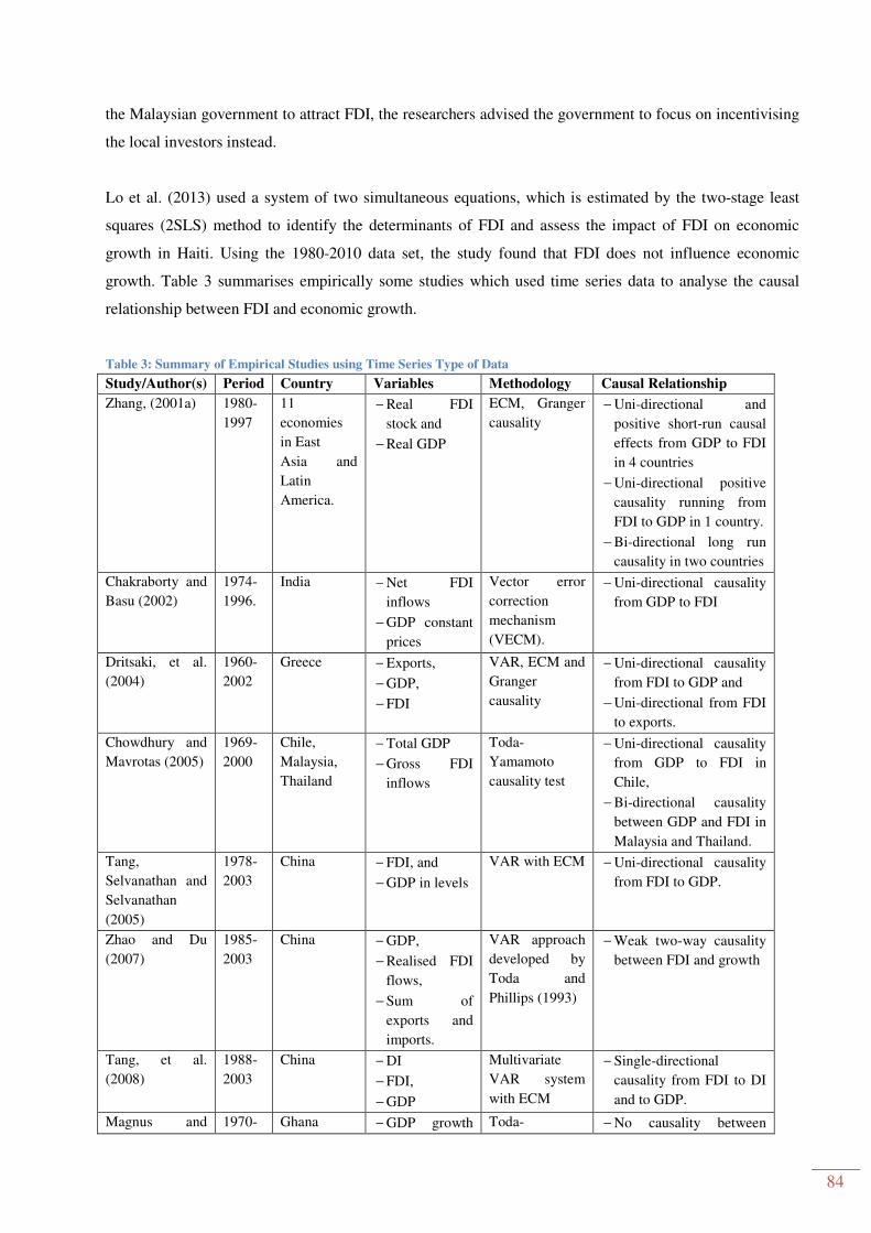
84
the Malaysian government to attract FDI, the researchers advised the government to focus on incentivising
the local investors instead.
Lo et al. (2013) used a system of two simultaneous equations, which is estimated by the two-stage least
squares (2SLS) method to identify the determinants of FDI and assess the impact of FDI on economic
growth in Haiti. Using the 1980-2010 data set, the study found that FDI does not influence economic
growth. Table 3 summarises empirically some studies which used time series data to analyse the causal
relationship between FDI and economic growth.
Table 3: Summary of Empirical Studies using Time Series Type of Data
Study/Author(s) Period Country Variables Methodology Causal Relationship
Zhang, (2001a) 1980-
1997
11
economies
in East
Asia and
Latin
America.
− Real FDI
stock and
− Real GDP
ECM, Granger
causality
− Uni-directional and
positive short-run causal
effects from GDP to FDI
in 4 countries
− Uni-directional positive
causality running from
FDI to GDP in 1 country.
− Bi-directional long run
causality in two countries
Chakraborty and
Basu (2002)
1974-
1996.
India − Net FDI
inflows
− GDP constant
prices
Vector error
correction
mechanism
(VECM).
− Uni-directional causality
from GDP to FDI
Dritsaki, et al.
(2004)
1960-
2002
Greece − Exports,
− GDP,
− FDI
VAR, ECM and
Granger
causality
− Uni-directional causality
from FDI to GDP and
− Uni-directional from FDI
to exports.
Chowdhury and
Mavrotas (2005)
1969-
2000
Chile,
Malaysia,
Thailand
− Total GDP
− Gross FDI
inflows
Toda-
Yamamoto
causality test
− Uni-directional causality
from GDP to FDI in
Chile,
− Bi-directional causality
between GDP and FDI in
Malaysia and Thailand.
Tang,
Selvanathan and
Selvanathan
(2005)
1978-
2003
China − FDI, and
− GDP in levels
VAR with ECM − Uni-directional causality
from FDI to GDP.
Zhao and Du
(2007)
1985-
2003
China − GDP,
− Realised FDI
flows,
− Sum of
exports and
imports.
VAR approach
developed by
Toda and
Phillips (1993)
− Weak two-way causality
between FDI and growth
Tang, et al.
(2008)
1988-
2003
China − DI
− FDI,
− GDP
Multivariate
VAR system
with ECM
− Single-directional
causality from FDI to DI
and to GDP.
Magnus and 1970- Ghana − GDP growth Toda- − No causality between

85
Study/Author(s) Period Country Variables Methodology Causal Relationship
Fosu (2008) 2002 rate
− FDI as a % of
GDP
Yamamoto
Granger no-
causality test
FDI and growth for the
total sample period and
the pre-SAP period,
− FDI Granger causes GDP
growth during the post-
SAP period.
Elboiashi, et al.
(2009)
1970-
2006
Egypt,
Morocco
and Tunisia
− Real GDP at
constant
prices
− % of FDI to
GDP
− GFCF
VEC,
Granger
causality
− Bi-directional causality
between FDI and GDP in
Tunisia,
− Uni-directional causality
from FDI to GDP in
Egypt, and
− Uni-directional causality
from GDP to FDI in
Morocco.
Jayachandran
and Seilan
(2010)
1970-
2007
India − Exports
− FDI and
− Real GDP
Cointegration
analysis and
Granger
causality test
− FDI Granger causes
exports,
− No causal relationship
from GDP to exports,
− No causal relationship
from GDP to FDI.
Majagaiya and
Gu(2010)
1980-
2006
Nepal − FDI,
− GDP growth
rate
OLS and
Granger
causality
Uni-directional from FDI to
GDP
Asheghian
(2011)
1976 -
2008
Canada − FDI
− GDP, TFP
Granger
causality in
time series
No causality
Feridun and
Sissoko(2011)
1976-
2002
Singapore − FDI
− GDP per
capita
VAR and
Granger
causality
Uni-directional from FDI to
economic growth.
Shaari, et al.
(2012)
1971-
2010
Malaysia − Real GDP and
− FDI in levels
VECM and
Granger
causality
Bi-directional causality
Ragimana
(2012)
1970-
2010
Solomon
Islands
− FDI, Exports,
and
− GDP per
capita
VECM and
Granger
causality
Long run bi-directional
causality between FDI and
GDP
Acaravci and
Ozturk (2012).
1994-
2008
10 transition
European
countries
− GDP at
constant
prices,
− Exports at
constant
prices and
− Ratio of FDI
to GDP
ECM, Granger
causality
Short and long-run causal
relation among the 3
variables in 4/10 countries
Lo, et al. (2013) 1980-
2010
Haiti − FDI as a % of
GDP
− Growth rate of
real GDP
Simultaneous
equations and
2SLS
No significant impact
Mohamed, et al. 1970- Malaysia − Real FDI VECM No causal relationship

86
Study/Author(s) Period Country Variables Methodology Causal Relationship
(2013). 2008. inflows
− Growth rate of
real per capita
GDP
between FDI and GDP in
both the short and long-run.
Source: Own compilation
3.3.3. Studies which used cross sectional data
Balasubramanyam, et al. (1996) estimated the growth-FDI link from a cross-section data for forty-six
developing countries over the period 1970-1985, using the OLS method. Their analysis showed a positive
impact of FDI on growth, but uniquely in countries that adopted an export promoting strategy. The study
stressed the importance of economic conditions and environment of the domestic country in enabling FDI
to have the greatest positive impact on GDP.
Hermes and Lensink (2003) conducted a cross-sectional study covering 67 countries for the period 1970-
1995. All the variables in the study were averaged. Their main objective was to demonstrate that a more
developed financial system enhances the positive relationship between FDI and economic growth. The
study found that of the 37 (out of 67) countries with a sufficiently developed financial system, FDI causes
economic growth. The paper concluded that a more developed financial system in the host country is an
important precondition for FDI to have a positive impact on economic growth (Hermes and Lensink,
2003:158).
In a similar study to Hermes and Lensink (2003), Alfaro, et al. (2004) studied the linkages between FDI,
financial markets and economic growth in a 71 country cross-sectional period from 1975-1995. The study
found that FDI alone plays an ambiguous role in contributing to economic growth, but with well-developed
financial markets, FDI Granger causes economic growth. The study recommended that countries should
not just focus on policies to attract FDI, but this should be done in conjunction with improvement of local
conditions, especially development of financial markets.
Sylwester (2005) conducted a study aimed at investigating how FDI affect GDP within a cross section of
less developed countries (LDCs) between 1970 and 1989. Though the study did not test for causality
directly, it inferred that owing to the strong positive association between FDI and economic growth, there
exists a possibility of causality from FDI to growth. The study also found that FDI not only promotes
economic growth but it doesn’t lead to unequal distribution of income.
Olofsdotter (1998) used the standard OLS method on cross-sectional data of fifty developing and
developed countries for the period 1980-1990. The study found that economic growth rate is affected by
87
the stock of FDI. It further concluded that FDI would have greater positive impact to growth in host
countries with strong institutional capacity.
3.3.4. Studies which used panel data
A study by Bronsztein, et al. (1998) is one of the initial papers to investigate how FDI can contribute to
economic growth. The study used a panel of sixty-nine developing countries for the period 1970-1989 and
employed seemingly unrelated regression (SUR) methods. The study found that FDI contributed positively
to economic growth. The study further found that FDI affects growth through technology diffusion, and it
emphasised that the host country’s labour force must have a certain level of education and competency for
the country to fully benefit from the technology and skills endowed in FDI (Bronsztein, et al., 1998:115).
However, Khawar (2005), in a study, which covered a cross section of countries over two decades, found
that FDI had a substantial and positive relationship with real income per capita, irrespective of any human
capital requirements of the host country.
In contrast, De Mello (1999) found evidence of a weak link between FDI and growth. His paper is based
on a sample of thirty-two OECD and non-OCED countries, from which seventeen were non-OECD
countries. The study used both time series and panel data for the period 1970-1990. The study further
concludes that the impact of FDI on growth depends on the complementarity and substitution between FDI
and domestic investment.
Nair-Reichert and Weinhold (2001), in a bid to allow for heterogeneity within countries, applied the mixed
fixed and random (MFR) coefficient approach in investigating the causal relationship between FDI and
economic growth. The study used panels of 24 developing countries from 1971 to 1995. The authors found
that on average there is a causal relationship from FDI to economic growth. As initially hypothesized, the
paper also found evidence that causal relationships across countries are ‘fairly heterogeneous’.
A study by Choe (2003) used the panel VAR model proposed by Holtz-Eakin, Newey and Rosen (1988),
normally referred to as HNR to test the causal relationship between FDI, DI and economic growth in 80
countries over the period 1971 to 1995. The study found that causality between FDI and economic growth
is bi-directional, with more compelling evidence of growth causing FDI than from FDI to growth.
Mencinger (2003) also tested the direction of causality between FDI and growth using a panel of 8
countries for the period 1994-2001, and found evidence of unidirectional causality from FDI to economic
growth.
Basu, Chakraborty, and Reagle (2003) used a panel vector error correction model (VECM) to explore the
two-way link between FDI and economic growth for a panel of 23 developing countries. The study covered

88
the period 1978 to 1996, and used the annual series for net FDI inflows and GDP as proxies for FDI and
economic growth respectively. The study found that short-run Granger causality was bidirectional and
long-run causality mainly runs from growth to FDI.
Another paper by Hansen and Rand (2006) analysed the Granger causal relationships between FDI and
GDP in a sample of 31 developing countries covering 31 years (1970-2000). The study employed bivariate
vector autoregressive (VAR) models for the log of GDP and the FDI ratio, and for the log of GDP and FDI
as a percentage of gross capital formation (Hansen and Rand, 2006:25). The authors find evidence of bi-
directional causality between the FDI-to-GDP ratio and the level of GDP, and conclude that FDI causes
growth in the long run.
Turkcan and Yetkiner (2008) tested the endogenous relationship between FDI growth and economic
growth using a panel dataset for 23 OECD countries for the period 1975-2004. The methodology used was
a two-equation simultaneous equation system with the generalised methods of moments (GMM). The study
found evidence of bi-directional relationship between FDI and economic growth, though “economic
growth stimulates growth rate of FDI inflows more strongly than that the growth rate of FDI stimulates
economic growth” (Turkcan and Yetkiner, 2008:12).
Liu, Shu and Sinclair (2009) used panel multivariate causality tests in VECM framework to test the causal
links between FDI, economic growth and trade in nine Asian countries over the period 1970-2002. The
results show evidence of a bi-directional causal relationship between trade, FDI, and GDP for the majority
of the countries in the sample. The study recommended that the Asian countries develop policies and
strategies aimed at promoting FDI, trade and economic growth concurrently. In the same year, Batten and
Vo (2009) used panel data modeling to investigate the link between FDI and GDP in 79 countries. The
later study found that FDI causes or positively impacts GDP, but the impact is stronger among countries
that have FDI. FDI also has a stronger positive impact on economies which have higher levels of
educational achievement, open trade, developed stock market, lower population growth rates and lower
levels of country risk (Batten and Vo, 2009:1638).
Ndoricimpa (2009) examined the interrelationship between FDI, exports and economic growth in 16
COMESA37 countries for the period 1983-2007. The main objective of the study was to test the “FDI-led
exports”, “Export-led growth” and “FDI-led growth” hypotheses in the COMESA region. The study tested
Granger causality was applied in heterogeneous panels using the Homogeneous Non-Causality and
Homogeneous Causality hypotheses as proposed by Hurlin and Venet (2001, 2003) and Hurlin (2004,
37 The 16 COMESA countries include Burundi, Comoros, DRC, Egypt, Ethiopia, Kenya, Libya, Madagascar, Malawi,
Mauritius, Seychelles, Sudan, Swaziland, Uganda, Zambia and Zimbabwe. Seven of them are SADC member
countries.

89
2007, 2008) and the Pooled Mean Group (PMG) estimation for Heterogeneous Causality tests. Some of the
findings of the Ndoricimpa (2009:87) study are that:
• Causality was unidirectional in 18.75% of the COMESA countries, running from FDI to Exports;
• Causality was unidirectional in 25.0% of the COMESA countries, running from Exports to FDI;
• Feedback causality in 50% of the COMESA countries; and
• No causality in 6.25% of the COMESA countries;
Lee and Chang (2009) used recent panel cointegration and panel error correction models (VECM) to test
for directions of causality among FDI, financial development, and economic growth. The empirical
analysis was applied on annual data of a set of 37 countries for the period 1970-2002. The proxies used for
the main variables were FDI net inflow as a percentage of GDP and real GDP in constant prices for FDI
and economic growth respectively. The study tested for both short run and long run causality. In relation to
FDI and economic growth, the study found evidence of a weak short-run causal relationship and strong
long-run bi-directional causality. The study also proved that an improvement in the domestic financial
system is important in channeling the positive externalities embodied in FDI inflows into economic growth
(Lee and Chang, 2009:268).
Esso (2010) examined the relationship between FDI and economic growth for ten Sub-Saharan African
countries. The study used the Pesaran, Shin and Smith (2001) approach to cointegration and the Toda and
Yamamoto (1995) non-causality test for the period 1970-2007. The causality results were that (i) FDI
Granger causes economic growth in three countries, (ii) economic growth Granger causes FDI in two
countries, and in the other countries there was no long-run relationship between the two variables.
Lund (2010) used the VECM framework to investigate the causal relationship between FDI and economic
growth using a data set of 128 countries for the period 1980-2003. Apart from direction of causality, the
study also investigated whether causality varies with income level of host country. The study sub-divided
the countries into low income, low middle, upper middle and high income. For all income groups, long-run
causality was found to be uni-directional; running from GDP to FDI. High-income countries showed
evidence of bi-directional causality in the short run, while for low and upper middle-income countries no
causality was found. The study found overwhelming evidence of GDP Granger causing FDI across all
income groups.
A study by Moudatsou and Kyrkilis (2011) investigates the causal-order between inward FDI and
economic growth for two different Economic Associations: European Union (EU) and Association of
South Eastern Asian Nations (ASEAN). The variables used are GDP per capita as a proxy for economic
growth and FDI as a percentage of gross fixed capital formation (GFCF) as proxy for FDI. The study used
panel data for the period 1970-2003 and employed the ECM estimation techniques. The overall conclusion

90
is that economic growth causes FDI in both developed and developing countries, and that there is weak bi-
directional relationship between the two variables across all countries.
Kotrajaras, Tubtimtong, and Wiboonchutikula (2011) used the standard panel Granger causality to examine
the relationship between FDI and economic growth in 15 East Asian countries. The data covered the period
1990-2009. The results showed that causation in most high and middle income countries ran from FDI to
economic growth, and FDI did not have significant effect on economic growth in low-income countries.
The study concluded that middle and high income countries generally have suitable economic conditions
that allow for the absorption of FDI, while low income economies are not able to absorb the spillovers or
technology being diffused by MNC from developed countries. Agrawal (2013) used the panel VEC
Granger causality test for FDI and GDP in BRICS countries over the period 1989-2012, and found
evidence of bi-directional causality between the two variables.
Mehraral, Haghnejad, Jalal Dehnavi and Mejbodi (2014) investigated the causal relationship among
economic growth, exports, and FDI inflows for 57 developing countries over the period of 1980 to 2008.
The study used per capita GDP in constant prices, and exports of goods and services as percent of GDP,
and per capita FDI inflow as proxies for the variables. After testing for integration and cointegration, the
researchers tested for Granger causality using the panel-based dynamic VECM in a multivariate
framework. The study results show that (i) exports and FDI Granger causes GDP in the short-run; (ii)
exports and FDI Granger cause GDP, and also exports and GDP Granger cause FDI in the long-run; and
(iii) GDP and FDI do not Granger cause exports in either the short run or the long run. The researches
recommended that countries should simultaneously implement outward-oriented strategies and policies of
attracting FDI and grow their economies as FDI and GDP have feedback effect.
Table 4 gives a summary of some empirical studies which used panel data to analyse the causal
relationship between FDI and economic growth.
Table 4: Summary of Empirical Studies on Panel Data
Study/Author(s) Period Countries Variables Methodology Causal Relationship
De Mello (1999) 1970-
1990.
32 OECD
and non-
OCED
countries
− Net FDI flows
− Per capita GDP
− Total factor
productivity
Both time series
and panel data
− Weak link between
FDI and growth
Nair-Reichert
and Weinhold
(2001).
1971-
1995
24
developing
countries
− FDI as a % of
GDP
− DI as a % of
GDP
− GDP in levels
Mixed fixed and
random (MFR)
panel causality
test
− Causal relationship
from FDI to economic
growth.
Choe (2003) 1971-
1995
80
countries
− growth rate of per
capita GDP
− FDI as a % of
Panel VAR
model proposed
by Holtz-Eakin,
− Causality between
FDI and economic
growth is bi-

91
Study/Author(s) Period Countries Variables Methodology Causal Relationship
GDP
− GDI as a % of
GDP
et al. (1988).
The HNR
method.
directional, with more
compelling evidence
of growth causing
FDI than from FDI to
growth.
Mencinger(2003) 1994-
2001
8 countries − FDI as a % of
GDP
− GDP growth
− Uni-directional
causality from FDI to
economic growth.
Basu, et al.
(2003)
1978-
1996
23
developing
countries.
− FDI inflows and
− GDP
Panel
cointegration
framework
− Short-run Granger
causality was bi-
directional, and
− Long-run causality
mainly runs from
growth to FDI.
Hansen and
Rand (2006)
1970-
2000
31
developing
countries
− FDI-to-GDP ratio
− FDI-to-GCF
− level of GDP
Heterogeneous
panel under a
VAR model
− Bi-directional
causality between
FDI/GDP and level of
GDP.
Turkcan and
Yetkiner (2008)
1975-
2004
23 OECD
countries
− FDI per capita
growth rates
− growth rates of
export per
− Growth rates of
per capita GDP
A simultaneous
equation
System, using
GMM
− Bi-directional
relationship between
FDI and economic
growth.
Sridharan, et al.,
(2009)
Different
periods
per
country
BRICS
(Brazil,
Russia,
India,
China, and
South
Africa)
− Industrial
Production Index
(IPI)
− FDI
VECM and
Granger
causality
− Growth leads FDI bi-
directionally for
Brazil, Russia and
South Africa and
− FDI leads Growth
uni-directionally for
India and China.
Lee and Chang,
(2009)
1970 -
2002
37
countries
− FDI as a % of
GDP
− Real GDP
− Domestic credit
as a % of GDP
− Liquid liabilities
as a % of GDP
Panel
cointegration
and panel error
correction
models (VECM)
− Weak uni-directional
causality from GDP
to FDI and FD in the
short run
− Strong bi-directional
causality between
GDP, FDI, and FD in
the long run.
Liu, et al. (2009) 1970-
2002.
9 Asian
countries
− Real FDI
− Real GDP
− Value of exports
& imports
Panel
multivariate
causality tests in
VECM
framework
− Bi-directional causal
relationship between
trade, FDI, and GDP
for majority of the
countries in the
sample.
Esso (2010) 1970-
2007.
10 Sub-
Saharan
African
countries.
− Real GDP per
capita
− FDI as a % of
GDP
The Pesaran, et
al. (2001)
approach to
cointegration
and the Toda
and Yamamoto
− FDI Granger causes
economic growth in
three countries,
− economic growth
Granger causes FDI
in two countries, and

92
Study/Author(s) Period Countries Variables Methodology Causal Relationship
(1995) − No long-run
relationship between
the two variables in
the other countries.
Lund (2010) 1980-
2003.
128
countries
− Real FDI stock
− Real GDP.
Panel VECM − GDP Granger causing
FDI across all income
groups in long-run.
− Bi-directional short-
run causality for high
income countries.
Kotrajaras, et al.
(2011)
1990-
2009.
15 East
Asian
countries.
− Panel Granger
causality test
− Causation ran from
FDI to economic
growth in most high
and middle income,
− FDI did not have
significant effect on
economic growth in
low-income countries.
Moudatsou and
Kyrkilis (2011)
EU and
ASEAN
countries.
− FDI as a % of
GFCF
− GDP per capita
Panel ECM
estimation
techniques.
− Economic growth
causes FDI in both
developed and
developing countries,
and
− Weak bi-directional
relationship between
the two variables
across all countries.
Abaidoo (2012) 1977-
2010
Sub-
Sahara
Africa
− FDI as a % of
GDP
− Real GDP growth
rate
− Savings as a % of
GDP
ECM and
trivariate
causality
methodology
− bi-directional
causality
Mehraral, et al.
(2014)
1980 -
2008.
57
developing
countries
− per capita GDP
− exports as % of
GDP
− per capita FDI
Panel vector
error correction
model (VECM)
− FDI Granger causes
GDP in the short-run;
− Bi-directional
causality between
FDI and GDP in the
long-run
Source: Own compilation
3.4. Conclusion
This chapter discussed the theoretical link between FDI and economic growth, and presented empirical
literature on the causal relationship between the two variables. The theoretical section started by defining
FDI before exploring the channels through which FDI affects economic growth. It was found that FDI is an
investment made to acquire lasting interest in enterprises operating outside of the economy of the investor

93
(IMF, 1993). FDI is mainly brought from an investing country by MNCs, and its motives are broad,
ranging from market seeking, resource seeking, and efficiency seeking or asset-seeking.
The theoretical exploration demonstrated that FDI is a key contributor to the economic growth of the host
country. Through exogenous and endogenous growth analysis, it was noted that FDI contributes directly
and indirectly to economic growth and that the host country’s growth may attract more FDI. It was also
observed that FDI affects economic growth through several channels, which De Mello (1997) broadly
categories into two: (i) FDI can encourage the adoption of new technologies in the production process
through technological spillovers, and (ii) FDI may stimulate knowledge transfers, both in terms of labour
training and skill acquisition and by introducing alternative management practices and better organisational
arrangements; commonly referred to as spillovers.
The impact of FDI on economic growth can be positive or negative depending on the channel or impact
mechanism. Studies by de Mello (1997 and 1999), UNCTAD (1999), OECD (2002) and Moura and Forte
(2010) emphasised that the impact of FDI on the host country’s economic growth is dependent on the
economic and technological conditions in the host country itself. These conditional factors include level of
human capital, the trading system, the degree of openness of its economy, investment policies and
legislation and political stability (Hansen and Rand, 2006; Chowdhury and Mavrotas, 2003 and Moura and
Forte, 2010).
The empirical literature review, on the other hand, discussed previous studies on the causal relationship
and link between FDI and GDP. Studies, which investigated the growth-driven FDI, FDI-led growth and
feedback or bi-directional causality, were reviewed. Most of the studies proved that high economic growth
rates were correlated with high investment rates. However results on causality are still mixed and
inconclusive. The majority of the studies showed evidence of unidirectional causality from FDI to
economic growth, while some found bi-directional causality. There are several explanations offered in
literature on the ambiguity of the results (Moura and Forte, 2010), and some of reasons include:
• Use of different variables (UNCTAD, 1999). For example some studies use stock of FDI, some
levels of FDI inflows while some use FDI as a percentage of GDP.
• Errors in estimation method (Nair-Reichert and Weinhold, 2001). As shown in the tables above, a
variety of methods ranging from simultaneous equations, OLS, different researchers employed
VAR, VECM and panel cointegration analysis.
• Lack of analysis of the host country’s domestic conditions. An analysis of literature by Moura and
Forte (2010:19) concluded that host country conditions such as levels of development, size,
political structure, and culture may have an effect on the impact and effect of FDI on the host
country’s economy.

94
In conclusion, the literature review has shown that FDI can positively impact the economy of the host
country through increasing capital and bringing in technology diffusion. However, its impact is dependent
on host country conditions such as the level of technology diffusion, and it emphasizes that the host
country’s level of education and competency should be high. Also important are economic, political, social
and cultural conditions. Thus, the host country government can play a leading role in both attracting FDI
and managing it to achieve the country’s developmental goals.
Lastly, a review of empirical literature reveals that researchers use different proxies for economic growth
and FDI. For economic growth the common proxies are per capita GDP, annual GDP growth rate, total
GDP and sometimes-total factor productivity. For FDI, most researchers use FDI as a % of GDP, FDI as a
% of GFCF and FDI stock. Seminal papers such as de Mello (1999) and Moudatsou and Kyrkilis (2011)
used GDP per capita as a proxy for economic growth while the majority of the papers for example Nair-
Reichert and Weinhold (2001), Choe (2003), Hansen and Rand (2006) and Esso (2010) used FDI as a % of
GDP as a proxy for foreign direct investment. However, because net FDI inflows in some SADC countries
are negative, this study used FDI stock and real GDP as proxies for the two variables, respectively (Zhang,
2001a).

95
CHAPTER 4: PRESENTATION OF THE METHODOLOGY
4.1. Introduction
This chapter presents the methodology and the model specifications of the study. The chapter is divided
into six subsections, namely: brief justification of the use of panel data methods on this study; empirical
model specification, which discusses in detail the two models used in this research; a presentation of the
recent panel unit root and cointegration tests.
4.2. Justification for using panel data
According to Baltagi (2008:1), panel data “refers to the pooling together of observations on a cross-section
of households, countries, firms, etc. over several time periods”. The letter ‘N’ represents the individuals in
the panel while the letter ‘T’ represents the time period. This study uses a macro panel of 15 SADC
countries for the period 1985 to 2012. As pointed out by Baltagi (2008), analysis of macro panel data is
normally faced with issues such as stationarity, unit roots, cointegration, and sometimes cross-country
dependence.
Hasio (2003), Gujarati (2004), and Baltagi (2008) offered advantages and benefits of using panel data over
time-series analysis, as briefly described below:
i. Panel data gives more informative data, more variability, less collinearity among the variables,
more degrees of freedom and more efficiency as compared to time-series or cross-sectional data
(Baltagi, 2008:7),
ii. Panel data provides control for individual heterogeneity. It is possible to control for individual
specific characteristics like colonial history, political regimes, geographical features, etc. and time-
invariant variables (Baltagi, 2008:6),
iii. Panel data is better suited for the study of dynamic adjustment (Baltagi, 2008:7),
iv. It is better able to identify and measure effects that are not detectable in pure cross-section or time-
series data in panel data (Baltagi, 2008:8),
v. Allows for the construction and testing of more complicated behavioral models (Baltagi, 2008:8),
such as economies of scale and technological change (Gujarati, 2004:639), and
vi. Because of more observations, panel data can reduce bias that might result from aggregation of
individuals into broad groups (Gujarati, 2004:639).
vii. Macro panel data eliminates the problem of non-standard distributions, which is typical of unit
roots tests in time series analysis (Baltagi, 2008).
96
Erdil and Yetkiner (2006) further argue that panel data provides a large number of observations, adds to the
degrees of freedom, lessens collinearity among explanatory variables and improves the efficiency of
Granger causality tests. Before we test for panel Granger causality, we first test for unit root in order to
determine the series’ order of integration and secondly perform cointegration tests to establish whether
there is any stable long-run relationship between FDI and economic growth. The unit roots and
cointegration tests are described in the next two sections respectively.
4.3. Empirical model specification
This study seeks to examine the direction of causality between FDI and economic growth in SADC
countries. Empirical literature shows that Granger (1969) causality is the most effective methodology in
investigating the interaction or causal relationships between variables. To investigate causality between the
two variables, a Granger (1969) causality test methodology is proposed. The Granger (1969) causality test
assumes that the information relevant to the predication of variable X and Y is contained solely in the time
series data on these variables. It argues that since the future cannot predict the past or a cause cannot
precede its effect, then variable X is said to Granger-cause variable Y if the current value of Y is
conditional on the past values of X. In regression of Y and other variables (including its own past or lagged
values), if we include past or lagged values of X and it notably improves the prediction of Y, then it is
suggested that X Granger causes Y. Similarly, Y can Granger cause X, by the same definition. In causality,
there are four possibilities, namely:
i. Unidirectional causality from X to Y,
ii. Unidirectional causality from Y to X,
iii. Feedback or bidirectional causality, and
iv. Independence.
In our case, we aim to determine whether FDI Granger causes growth (which tests the FDI-led growth
hypothesis); economic growth attracts FDI (which tests the growth-driven FDI hypothesis) or the
possibility of the two variables influencing each other through the feedback effect.
In this sub-section, we discuss different forms of model specifications depending on the statistical
properties of the variables, in terms of stationary and cointegration. We start by putting forward the
standard Granger causality test framework.

97
4.3.1. Standard Granger causality test
A simple bi-variate panel Granger (1969) causality test involves the estimation of the two equations below
(Equation 5 and 6). This test is an extension of time series analysis (see Al Nasser, 2010; Fowowe, 2011;
and Zhang, Wang and Zhu, 2012 for more details).
���� = � +∑ � � !� ���� +∑ " � !� #�$� +%� [5]
#�$� =�� +∑ �� � !� #�$� +∑ �" � !� ���� +%" [6]
Where GDP is economic growth and FDI is foreign direct investment. � and �� are intercepts for
Equation 5 and 6 respectively, so are the two white noise error terms %� and %" . The null hypotheses to be
tested are shown below (see Al Nasser, 2010).
i. ∑ " � !� = 0, which implies that GDP does not Granger cause FDI; and
ii. ∑ �" � !� = 0, which implies that FDI does not Granger cause GDP.
The above two hypotheses can be tested using the F-test (Fowowe, 2011:223). However, the specifications
in Equations 5 and 6 change if the two variables are non-stationary. Fowowe (2011) suggests that after
testing for unit roots, the causality tests can proceed in either of the two ways: (i) if variables are integrated
of the same order [I(1)] and are co-integrated, then the error correction model (ECM) as proposed by
Granger (1988b) is used; (ii) if the variables are not co-integrated, Granger causality can still proceed by
vector autoregressions (VARs). Please see Toda and Phillips (1993), Hurlin and Venet (2001, 2008) and
Fowowe (2011:223-224).
4.3.2. Vector Autoregressions (VAR)
Dumitrescu and Hurlin (2012) argue that heterogeneity in panel data models is from two sources. The first
is the presence of distinctively different intercepts or presence of individual effects between individuals in
the panel. This heterogeneity is normally addressed through the estimation of panel fixed effects models
(Baltagi, 2008). The second source of heterogeneity is causal variation across cross-sections, also referred
to as heterogeneity of parameters or coefficients (�� in Equation 7 below). The second heterogeneity was
overlooked in conventional panel causality models such as Hsiao (1986, 2003) among others, and has been
the subject of recent investigations by Nair-Reichart and Weinhold (2001), Hurlin and Venet (2001),

98
Hurlin (2004, 2008), and Dumitrescu and Hurlin (2012). As discussed herein, the Dumitrescu and Hurlin
(2012) test takes into account both dimensions of heterogeneity.
The test allows for heterogeneous panel data with fixed, as opposed to time-varying coefficients. Assuming
a bivariate set-up, the test is based on the following linear model:
(�, = � + )*����+
�!�(�,�� +)�����
+
�!�,�,�� +%�, [7]
Dumitrescu and Hurlin (2012) propose a simple test of the HNC hypothesis under the null of “there is no
causal relationship for any units of the panel” against an alternative of “there is a causal relationship from ,
to ( for a subcategory of individuals in the panel”. This approach takes into account both the heterogeneity
of the regression model and that of the causal relationship, as stated below.
-.: �� = 0 ∀� = 1,…2, and
-3: �� = 0 ∀� = 1,…2�
-3: �� ≠ 0 ∀� = 2� + 1, 2� + 2,…2
Where �� = ������, ���"�, …���+�)´, 2� is unknown but it’s less than 2. If 2� = 2 it means there is no
causality in any of the panels, but if 2� = 0 there is evidence of causality in all the individuals in the
sample. Acceptance of the null hypothesis (HNC) means variable , does not Granger cause variable ( for
all the individuals of the panel. Rejection of the null of HNC where 2� = 0 means that , Granger causes
( for all the individuals of the panel, and thus we have an homogeneous causality result. However if the
null is rejected and 2� > 0 , it means the causality relationship is heterogeneous. This third case implies
that the regression model and the causality relations are distinct from one unit in the panel to another.
The only condition for the Dumitrescu and Hurlin (2012) is that variables should be stationary. However
several studies, such as Zhang (2001a), Moudatsou and Kyrkilis (2011), Fowowe (2011), Emirmahmutoglu
and Kose (2011) and Cao and Jariyapan (2012) have argued that if the variables are co-integrated then
Granger non-causality tests should be conducted using the error correction model (ECM) as proposed by
Granger (1988b).
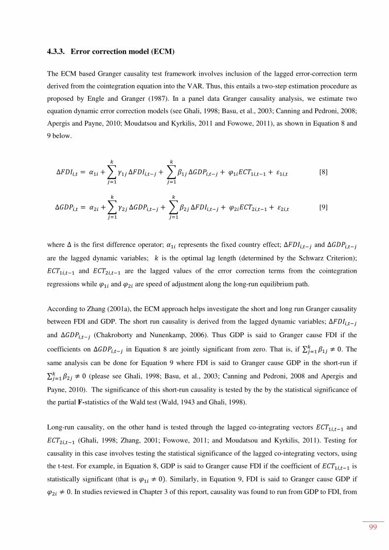
99
4.3.3. Error correction model (ECM)
The ECM based Granger causality test framework involves inclusion of the lagged error-correction term
derived from the cointegration equation into the VAR. Thus, this entails a two-step estimation procedure as
proposed by Engle and Granger (1987). In a panel data Granger causality analysis, we estimate two
equation dynamic error correction models (see Ghali, 1998; Basu, et al., 2003; Canning and Pedroni, 2008;
Apergis and Payne, 2010; Moudatsou and Kyrkilis, 2011 and Fowowe, 2011), as shown in Equation 8 and
9 below.
∆����, = �� +)*� �
!�∆����,� +)��
�
!�∆#�$�,� +7��89:��,�� +%��, [8]
∆#�$�, = "� +)*" �
!�∆#�$�,� +)�"
�
!�∆����,� +7"�89:"�,�� +%"�, [9]
where ∆ is the first difference operator; �� represents the fixed country effect; ∆����,� and ∆#�$�,� are the lagged dynamic variables; ; is the optimal lag length (determined by the Schwarz Criterion);
89:��,�� and 89:"�,�� are the lagged values of the error correction terms from the cointegration
regressions while 7�� and 7"� are speed of adjustment along the long-run equilibrium path.
According to Zhang (2001a), the ECM approach helps investigate the short and long run Granger causality
between FDI and GDP. The short run causality is derived from the lagged dynamic variables; ∆����,�
and ∆#�$�,� (Chakroborty and Nunenkamp, 2006). Thus GDP is said to Granger cause FDI if the
coefficients on ∆#�$�,� in Equation 8 are jointly significant from zero. That is, if ∑ �� � !� ≠ 0. The
same analysis can be done for Equation 9 where FDI is said to Granger cause GDP in the short-run if
∑ �" � !� ≠ 0 (please see Ghali, 1998; Basu, et al., 2003; Canning and Pedroni, 2008 and Apergis and
Payne, 2010). The significance of this short-run causality is tested by the by the statistical significance of
the partial F-statistics of the Wald test (Wald, 1943 and Ghali, 1998).
Long-run causality, on the other hand is tested through the lagged co-integrating vectors 89:��,�� and
89:"�,�� (Ghali, 1998; Zhang, 2001; Fowowe, 2011; and Moudatsou and Kyrkilis, 2011). Testing for
causality in this case involves testing the statistical significance of the lagged co-integrating vectors, using
the t-test. For example, in Equation 8, GDP is said to Granger cause FDI if the coefficient of 89:��,�� is
statistically significant (that is 7�� ≠ 0�. Similarly, in Equation 9, FDI is said to Granger cause GDP if
7"� ≠ 0. In studies reviewed in Chapter 3 of this report, causality was found to run from GDP to FDI, from

100
FDI to GDP, in both directions or in neither direction for both short-run and long-run. This is in line with
the causality theory.
Thus, before running Granger causality tests based on specifications in Equations 8 and 9 above, it is
important to test for unit roots and cointegration. Section 4.5 and 4.6 below gives a summary of tests of
panel unit roots and cointegration respectively, based on recent literature.
4.4. Data sources and definitions of variables
In order to investigate the causal relationship between FDI and economic growth, we used panel data
analysis framework. The sample covers 15 SADC countries from 1980-2012. The sample period is
determined mainly by the availability of data, but it also coincides with the massive reforms by the SADC
countries aimed at attracting FDI (see Chapter 2 of this study). During this period, SADC as a regional bloc
and individual countries explicitly pursued policies aimed at attracting FDI such as economic liberalisation,
privatisation, instituting government funded agencies to attract investment, establishment of special
economic zones and offering of incentives and tax holidays to foreign investors.
A review of empirical literature (see Chapter 3 of this study) reveals that researchers use different proxies
for economic growth and foreign direct investment. For economic growth the common proxies are per
capita GDP, annual GDP growth rate, total GDP and sometimes total factor productivity. For foreign direct
investment on the other hand, most researchers use FDI inflows as a % of GDP, FDI as a % of GFCF and
FDI stock. Seminal papers such as Zhang (2001a) and Lund (2011) used FDI stock as a proxy for foreign
direct investment and real GDP as a proxy for economic growth. This study uses the same proxies as
shown in Table 5.
Table 5: Variables used in this study
Number Acronym Variable Description Source
1 FDI FDI Stock: US Dollars at current prices and current exchange rates in millions.
World Investment Report (WIR) and United Nations on Trade and Development (UNCTAD) database (www.unctadstat.unctad.org).
2 GDP Real GDP: US Dollars at constant prices (2005) and constant exchange rates (2005) in millions.
United Nations on Trade and Development (UNCTAD) database (www.unctadstat.unctad.org).

101
4.5. Panel unit roots tests: Review of recent literature
Broadly, there are two groups of panel unit root tests. The first assumes a common unit root process, that
is, it assumes homogenous autoregressive coefficients between the cross-sections. These include the tests
developed by Hadri (2000); Breitung (2000); and Levin, Lin and Chu (LLC, 2002). The other group
assumes individual unit roots, with the assumption that the first order autoregressive parameter varies with
cross-sections. This second group includes the Im, Pesaran and Shin (IPS, 2003); Madala and Wu (MW,
1999) and Choi (2001). All the other tests test the null hypothesis of non-stationarity (or unit root) except
Hadri (2000) which tests the null hypothesis of stationarity.
4.5.1. Levin, Lin and Chu (LLC) (2002)
The LLC test allows for possible correlation and heteroskedasticity, though still assuming continued
independence across cross-sections. The null hypothesis under the LLC is that each individual time series
contains a unit root against the alternative that each time series is stationary, stated as:
-.: Each individual time series contains a unit root
-3: Each time series is stationary
LLC suggests a 3-step testing procedure as follows which involves running a separate augmented Dickey-
Fuller regression for each cross-section (Equation 10); estimating the long-run to short-run standard
deviations and computing panel test statistics (Equation 11). Please see Levin, et al. (2002), Baltagi
(2008:276) and Greene (2012:1011).
∆(�, = <� (�,�� +)=�>?�
>!�∆(�,�> +∝@� A@ +%�,, forE = 1,2,3. [10]
where dmt denotes the vector of deterministic variables, <� is the lag-order which is permitted to
vary across cross-sections and is determined by choosing a <@GH and then use a t-statistic of =�>;
εi,t is assumed to be independently distributed across i and t, i = 1,..., N, t = 1,..., T. The normalised
bias and the pseudo t-ratio that corresponds with the pooled OLS estimation of δ in (Equation 10),
once they have been properly normalised, converge to a standard Normal limit distribution as N
→ ∞, T → ∞ in a way that .
0/ →TN

102
The LLC adjusted t-statistic is:
IJ∗ = K–MNOPQMRSTURV �KV�WXNO∗
YXNO∗ ~2�0,1� [11]
As T and N turns to infinity, IJ∗approaches a normal distribution. Using a one tail test, we reject the null
hypothesis if test statistic is smaller than the critical value (-1.645) or if p< 0.05.
According to Baltagi (2008:277), the LLC test has its limitations, which include its dependence upon the
independence assumption across cross-sections. This makes the test inapplicable in the presence of cross-
sectional correlation. Secondly, the assumption that all cross-sections are non-stationary is limiting.
4.5.2. IM, Pesaran and Shin (IPS) (2003)
The Im, et al. (2003) (IPS) test allows for the heterogeneous coefficient of (�,�� (see Equation 10) and
proposes an alternative testing procedure to the one for LLC. The IPS testing procedure is based on the
averaging of individual augmented Dickey-Fuller (ADF) unit root test statistics. The IPS allows for
concurrent stationary and non-stationary data series, works on balanced panels and uses a likelihood-
testing framework (Ndoricimpa, 2009). The IPS is the same as the LLC model (Equation 10) in that it runs
separate ADFs for each cross-section (that is for each �).
The null hypothesis is that each series in the panel contains a unit root and the alternative hypothesis allows
for some (but not all) of the individual series to have unit roots. The null and alternative hypothesis under
the IPS is stated as follows:
-.: Each series in the panel contains a unit root (<� = 0∀�) -3: Some (but not all) of the individual series have unit roots (<� < 0for at least one �).
As stated above, the IPS t-bar statistic is defined as the average of the individual ADF statistics as shown in
Equation 12 below (Baltagi, 2008:279).
I̅ = �^ ∑ IJ_�̂!� [12]
Where IJ_ is are individual t-statistics for testing -.: <� = 0. The IPS assumes that IJ_ are independent and
identically distributed (iid) and have finite mean and variance.

103
A standardised final test statistic under the IPS is as follows (as in Baltagi, 2008:279):
I`?a =b�cGd =√2�I̅ − 12∑ 8�̂!� [I�g <� = 0]i �j1�∑ klm�̂!� [I�g <�i = 0]
[13]
Where 8[I�g <�i = 0] and klm[I�g <�i = 0] are means and variances respectively. These IPS means and
variances are computed based on Monte Carlo simulated moments or experiments, based on different lag
orders (n�), different values of T and the deterministic structure of the ADF test performed (according to
the Table in Im, et al., 2003:66).
The IPS test assumes that : → ∞ followed by 2 → ∞ sequentially, and I`?a ⇒ 2�0,1�. In a left or lower
tail test, we reject the null hypothesis if the test statistic is smaller than the critical value (-1.645), or if
p< 0.05.
Two main advantages of the IPS over the LLC are that it has better smaller sample properties and is more
intuitive in its construction (Baltagi, 2008:279). The disadvantage is that if we reject the null hypothesis,
the IPS test does not provide guidance on the size of the standard deviation (r� or the identity of the
specific individuals in the panel whose null hypothesis has been rejected. Furthermore, special care has to
be exercised in the interpretation of the results, as rejection of the null hypothesis does not necessarily
mean that the unit root null is rejected for all individuals (�), but only for some members of the group
(which is 2� < 2) (Ndoricimpa, 2009).
4.5.3. Breitung (2000) test
Both the LLC and IPS require that 2 → ∞ and 2 :i → 0 , that is 2 should be small enough relative to :.
However, simulations results show that both IPS and LLC have size distortions when 2 is small or when 2
gets large relative to : (Baltagi, 2008:280; Im et al., 2003; and Breitung, 2000).
The null and alternative hypothesis under the Breitung test are the same as that of LLC. The null
hypothesis requires that < be homogenous across �.
-.: Each individual time series contains a unit root
-3: Each time series is stationary

104
Breitung (2000) found that LLC and IPS suffer from loss of power if individual-specific trends are
included; this is due to bias correction that also removes the mean and the sequence of local alternatives
(Baltagi, 2008:280). Baltagi (2008) further notes that the LLC and IPS tests are sensitive to specification of
deterministic terms. As a result, Breitung (2000) suggests a test that does not employ a bias correction, and
with significantly higher power.
Just like the LLC, the Breitung test also follows a 3-step testing procedure. But instead of ∆(� , ∆(�,�>
(see Equation 10 above) is used in obtaining residuals. The calculated residuals are transformed using a
forward orthogonalisation transformation before being recalculated using a pooled regression (Baltagi,
2008:280).
The resultant t-statistic for -.: <� = 0 has in the limit, a standard normal distribution [ 2�0,1�]. There are
no kernel computations required (Baltagi, 2008:280). Furthermore, as 2, : → ∞, the Breitung test statistic
(Is̅g) ⇒ 2�0,1�. In a one tail test, we reject the null hypothesis if the test statistic is smaller than the
critical value (-1.645) or if p< 0.05.
4.5.4. Fisher-ADF and Fisher-PP [Madala and Wu (1999) and Choi (2001)] tests
These two tests, like the Breitung test, focus on the shortcomings of the LLC and IPS. Madala and Wu
(1999) and Choi (2001) suggest a non-parametric Fisher-type test based on a combination of the p-values
of the test-statistics for a unit root in each cross-sectional unit (Ndoricimpa, 2009:63). Some of the
characteristics of the Fisher-ADF and Fisher-PP and comparisons with the LLC and IPS are listed below
(Baltagi, 2008:281):
• The IPS assumes that : is constant for all �, while the Fisher-ADF test does not require a balanced
panel.
• While the IPS and LLC are fundamentally based on the ADF test, the Fisher-ADF and Fisher-PP
can accommodate different unit root tests. Besides, the Phillips-Perron (PP) tests (Philips and
Perron, 1988) can also be used on individual cross-sections.
• The Fisher-ADF and Fisher-PP can accommodate heterogeneity across cross-sections, that is,
different <�s.
• The Fisher-ADF and Fisher-PP assume very limited possible dependence across individuals (�). • The Fisher-ADF and Fisher-PP can be adapted for less restrictive assumptions about cross-
correlations (bootstrap techniques).
• The test however requires Monte Carlo simulations based on p-values.
The null and alternative hypotheses are defined similar to IPS, thus:

105
-.: Each series in the panel contains a unit root (<� = 0∀�) -3: Some (but not all) of the individual series have unit roots (<� < 0for at least one �).
Madala and Wu (1999) proposed a Fisher (1932) based test that combines information on the unit root test
p-values38. The proposed Fisher-type test, as explained in Baltagi (2008) and Greene (2012:1011) is as
follows:
$ =−2∑ ln n��̂!� ~v"^" [14]
With n� as the n-value for the unit root test performed on the cross-section �. This Madala and Wu (1999)
test has the advantage that it is an exact test; that is it doesn’t depend on the asymptotics for distribution,
like other tests. Secondly, given n-values, the test is straight forward. However, finding the n-values may
be difficult and might require simulation post testing (Baltagi, 2008:281).
As :� → ∞ for finite 2, the Madala and Wu (1999) test statistic (I?̅) ⇒v"^" , therefore we reject the null
hypothesis of non-stationarity if $ > $wd��wG�xG�yzor if p< 0.05.
In addition, Choi (2001) demonstrates that:
{ = �√^∑ Φ���n��̂!� � ~2�0,1� [15]
Where �� is the inverse of the standard normal cumulative distribution function. Both the asymptotic v"^"
and the normal [2�0,1�] distribution statistics of the Fisher-ADF and Fisher-PP individual unit roots are
reported in E-views.
4.5.5. Hadri (2000) test
The Hadri (2000) test is a residual based Lagrange multiplier (LM) test. Unlike the other five tests
discussed above, the Hadri test evaluates the null hypothesis of stationarity.
-.: No unit roots in any of the series in the panel.
-3: All series contain unit roots.
38 In general, the Fisher (1932) test is constructed around repeated observations on p-values.

106
The Hadri test is based on the residual from the individual ordinary least squares (OLS) regressions of (� on a constant or on a constant and a trend. For example, if we include both the constant and a trend, the
estimates are derived from:
(� =m� +��I + %� [16]
where m� =m�,�� +}� is a random walk, and
%� ~��2�0, r~"�, and }� ~��2�0, ry"�.
Using back-substitution (putting the random walk in Equation 16 and re-writing) will result in (Baltagi,
2008):
(� =m�� +��I +∑ }�� +�!� %� = m�� +��I + k� [17]
The stationarity hypothesis may therefore be written as
-.: ry" = 0, in which case %� =k� -3: ry" ≠ 0.
According to Baltagi (2008), Greene (2012) and Smith (2000), the LM statistic under the assumption of
homoscedasticity across cross-sections is given by:
��� = �^ �∑ �gU�̂!� ∑ ��"g!� �/r�~" [18]
Where �� =∑ %�̂��!� is the partial (cumulative) sum of OLS residuals, r�~" is a consistent estimator of r~"
under the null, with a potential candidate r�~" = �^g ∑ ∑ %�̂"g!��̂!� .
Hadri (2000) also suggests an alternative LM test that allows for heteroskedasticity across � say r~�" , as
follows (also outlined in Smith, 2000 and Baltagi, 2008):
��" = �^ �∑ � �gU�̂!� ∑ ��"g!� �/r�~")) [19]
The test statistic is then given by:
{ = √^�>����� ⇒ N (0,1) [20]

107
With � = 1 6i and � = 1 45i if the model only includes a constant and � = 1 15i and � = 11 6300i if the
model includes a constant and a trend. E-views computes both statistics (��� and ��"). We reject the null
hypothesis if p< 0.05 or magnitude of the test statistic is greater than 1.96, and conclude that the panel is
non-stationary.
4.6. Panel cointegration tests: Review of recent literature
According to Baltagi (2008), panel cointegration models are normally used to study long-run
macroeconomic relationships. The notion of cointegration therefore suggests the existence of a long-run
relationship between economic variables. If the variables are said to be co-integrated, it means that they
move together over time so that short-term disturbances are corrected in the long-run (Ndoricimpa, 2009).
Cointegration is most often associated with economic theories that imply equilibrium relationships between
time series variables. Variables must usually be integrated of the same order [I (d)] to form a co-integrating
relationship.
Reminiscent of the panel unit root tests described in the above section, panel cointegration tests have been
developed over the past few years with the motive of coming up with more powerful tests to those once
used in time series analysis. Broadly, the panel cointegration tests are two groups: those which are residual
based and the likelihood-based tests. Of the residual tests, first group assumes a null hypothesis of ‘no
cointegration’ while the other assumes ‘cointegration’. The tests which are used in this study are briefly
described below.
4.6.1. Residual-Based DF and ADF tests (Kao, 1999)
As the name suggests, Kao (1999) developed a residual-based panel cointegration test. The test is based on
a homogenous panel, and assumes a common co-integrating vector. The test includes the derivation of
Dickey-Fuller (DF) tests ( Dickey & Fuller, 1979;1981) and an augmented Dickey-Fuller (ADF); residual
error correction coefficient (<) and t-statistics. A detailed discussion is in Smith (2000), Baltagi (2008) and
Greene (2012).
In the null hypothesis, the residuals are non-stationary (that is, there is no cointegration). In the alternative
hypothesis, the residuals are stationary (that is, there is a co-integrating relationship among the variables).
-.: No cointegration (< = 1� -3: Cointegration.

108
Kao (1999) proposes four different DF-type of statistics as well as one ADF-type statistic. The first two
DF-types of statistics test for cointegration based on the strong exogeneity of the regressors and errors,
while the second set test cointegration with endogenous relationship between regressors and errors. Both
the DF-type and ADF-type statistics follow an asymptotic distribution which converges to a standard
normal distribution [N�0,1�] by sequential limit theory.
4.6.2. Panel ADF and PP tests (McCoskey and Kao, 2001)
The MacCoskey and Kao (2001) panel ADF and PP tests, unlike the Kao (1999) discussed above, are
based on heterogeneous panel data models. That is, they allow each individual cross section to have its
own co-integrating vector. They assume the null hypothesis of ‘no cointegration’.
-.: No cointegration
-3: Cointegration.
The testing process involves constructing ‘in style’ as in the IPS test for unit root. The calculations are
based on the average of individual cointegration test statistics and then normalised with appropriate mean
and variance for standard normal limiting distribution [as per the MacCoskey and Kao (1997:31) table].
The MacCoskey and Kao (2001) proposed moments (mean and variance) allow for intercept but no time
trend. These moments are based on Monte Carlo simulations with 50 000 replications. The final test
statistic is based on a one-tail test (lower tail of the distribution), and is calculated as follows (see Baltagi,
2008):
Test Statistic = √^�̅����@zG��
�� or √^�??�����@zG��
�� [21]
We obtain the average ADF or average PP from normal unit root testing procedures in Eviews, then adjust
with simulated values for mean and standard deviation in the MacCoskey and Kao (1997:31) table. We
then compare with standard normal critical values (one-sided test). If the test statistic is lower than the
critical value (-1.645) we reject the null hypothesis of a unit root and conclude that the residuals are
stationary and the variables in the long-run relationship are co-integrated.
4.6.3. Pedroni (1999, 2004) panel cointegration tests
Pedroni (1999, 2004) proposes a set of seven tests for the null hypothesis of ‘cointegration’ in a panel data
model that allows for significant heterogeneity. The Pedroni tests can be divided into two broad categories;
the first group falls under residual-based LM tests, which involves taking an average of the test statistics

109
for cointegration in the time series within cross-sections. This group of tests is termed “within
dimensions”, and it includes the panel-v, panel-rho(r), panel non-parametric (pp) and panel parametric
(ADF) statistics. These tests are similar to the single equation ADF-test.
The second group is referred to a “between dimensions”. This group includes group-rho, group-pp, and
group-ADF statistics. The test statistics involve the averaging in pieces such that the limiting distributions
are based on limits of piecewise numerator and denominator terms (Baltagi, 2008:295), and this is
equivalent to the IPS (2003) group mean panel unit root tests. Overall, the Pedroni (2004) test is actually a
panel extension of the Engle Granger (1987) two-step method of testing for cointegration, and relies on
ADF and PP principles.
-.: No cointegration (-.:<� = 1, ∀�) -3: Cointegration (-3:<� < 1, ∀�)
The null hypothesis tested is whether <� is unity (<� = 1�. All the seven test statistics are normally
distributed. The statistics can be compared to appropriate critical values in the standardised normal
distribution tables (Gujarati, 2004). If the calculated test statistics are greater that the critical values (or p-
value is smaller than ∝), then the null hypothesis of no cointegration is rejected, meaning that that a long-
run relationship between the two variables exists. However, of the seven tests panel-v is an exception in
that it rejects the null of cointegration when it has a large positive value (the others reject the null of no
cointegration when the calculated test statistic is large and negative). According to Pedroni (2004), rho and
pp tests tend to under-reject the null of no cointegration in case of smaller samples.
Furthermore, rejection of the null hypothesis under the Pedroni (1999, 2004) tests imply that “enough of
the individual cross-sections have statistics ‘far away’ from the means predicted by the theory were they to
be generated by the null” (Baltagi, 2008:296). Under the alternative hypothesis, panel-v statistics diverges
to positive infinity. Thus, panel-v is a one sided test where large positive values reject the null of no
cointegration. For each of the other six test statistics, these diverge to negative infinity under the alternative
hypothesis, and consequently the left tail of the normal distribution is used to reject the null hypothesis.
Thus, for any of these latter tests, large negative values imply that the null of no cointegration is rejected
(Pedroni, 2004:668).
4.6.4. Johansen and Fisher panel cointegration tests (Madala and Wu, 1999).
Madala and Wu (1999) developed a Johansen-type panel cointegration test. The Madala and Wu (1999)
test uses the Fisher (1932) result that is why it is sometimes referred to as the Johansen-Fisher test. The
testing approach combines tests from individual cross-sections to obtain at test statistic for the full panel.

110
The Madala and Wu (1999) test results are based on p-values for Johansen's cointegration trace test and
maximum eigenvalue test (Baltagi, 2008:297).
The tests evaluates null hypotheses of ‘no cointegration’ at different levels (r = i), which can be stated as
‘no cointegration’, ‘at most one cointegration relationship’, ‘at most 2 cointegration relationships’, etc.
In summary, this chapter presented a review of recent literature on panel data analysis involving non-
stationary data. It discusses several recent panel unit root and cointegration tests. The chapter then argues
that depending with the results of the panel unit roots and cointegration tests, two possible Granger
causality estimation techniques could be applied; the VAR or the ECM methodology. One possible VAR is
the one proposed by Dumitrescu and Hurlin (2012). This test requires that the variables be stationary, and
it takes into account both the heterogeneity of the causal relation and the heterogeneity of the regression
model used to test for Granger causality within a panel framework. If the variables are found to be non-
stationary and co-integrated, causality will be tested using the ECM framework (Granger, 1986 and 1988b;
Urbain, 1992; Ghali, 1998; and Pesaran, et al., 1999).

111
CHAPTER 5: EMPIRICAL ANALYSIS OF THE CAUSAL RELATIONSHIP
BETWEEN FDI AND ECONOMIC GROWTH IN SADC COUNTRIES
5.1. Introduction
This chapter presents the empirical analysis and results of the study. The chapter is structured according to
the estimation procedures followed. Panel unit roots are conducted first to test for stationarity and order of
integration of the variables. The study used IPS (2003) and PP-Fisher PP-Fisher panel unit root tests. Panel
cointegration tests were then performed on the two variables using the Pedroni (1999 and 2004) and Kao
(1999) panel cointegration tests.
In order to assess whether the causal relationship between FDI inflows and economic growth is dependent
on the level of income, the study divided the SADC countries into two groups, namely, the low-income39
and the middle-income40 countries. The classification was done in accordance with the World Bank (2012)
rankings. The two SADC low-income and middle-income groups have six and nine countries respectively.
The panel unit root, cointegration and Granger causality tests are presented according to the two income
country groups.
5.2. Descriptive analysis
Table 6 shows the descriptive statistics for the data in terms of mean, median, minimum, maximum and
standard deviation of the variables. From Table 6, the annual stock of FDI in SADC had a mean value of
US$896.48 million over the study period (1985-2012). The minimum annual FDI stock was US$0.112
million while the maximum was US$21 331.81 million. The standard deviation is 2 445.34. This implies
that the increase in FDI stock in the SADC region was varied across the sampled countries. This is
expected given individual uniqueness of the SADC countries as discussed in Chapter Two of this study.
With regard to real GDP, the values in Table 6 show that mean value for the entire sample was
US$20 518.80 million. During the same period, one of the countries had the lowest GDP of US$472.54
million (which is the smallest economy) and maximum of US$305 billion41. From Table 6, it can be
concluded that there is a large variation in FDI stock and GDP levels among SADC countries.
39 SADC low-income countries: Democratic Republic of Congo (DRC), Madagascar, Malawi, Mozambique, Tanzania
and Zimbabwe. 40 SADC middle-income countries: Angola, Botswana, Lesotho, Mauritius, Namibia, Seychelles, South Africa,
Swaziland and Zambia. 41 By 2012 the smallest SADC country was Seychelles while the biggest was South Africa.

112
Table 6: Descriptive statistics of variables
Variables FDI GDP Mean 896.4763 20518.80 Median 226.707 5591.173 Maximum 21331.810 305544.80 Minimum 0.112 472.541 Standard Deviation 2445.342 53329.56 Observations 420 420
Source: Own calculations from UNCTAD (2013a) Databases
As shown in the Figures 25, 26, 27 and 28 below, there has been a general increase in stock of FDI into all
SADC countries, except in Angola and Botswana, which have experienced sharp declines in recent years
(see Chapter 2 for detailed country by country discussions). The total GDP of individual SADC countries
has also been increasing over the study period, though the DRC and Zimbabwe reported sharp declines in
the last ten years.
The first two graphs below show the values of FDI stock and real GDP by country for the SADC middle-
income countries. The next set shows the same graphs for the low-income countries.
Figure 25: FDI Stock in Middle Income Countries 1980-2012 (US Millions)42
Source: Own calculations from UNCTAD (2013a) Databases
42 Key: FDI=FDI stock, ANG=Angola, BOT=Botswana, LES=Lesotho, MAU=Mauritius, NAM=Namibia,
RSA=Republic of South Africa, SEY=Seychelles, SWA=Swaziland, and ZAM=Zambia.
0
4,000
8,000
12,000
16,000
1980 1985 1990 1995 2000 2005 2010
FDI_ANG
400
800
1,200
1,600
2,000
1980 1985 1990 1995 2000 2005 2010
FDI_BOT
0
200
400
600
800
1,000
1980 1985 1990 1995 2000 2005 2010
FDI_LES
0
1,000
2,000
3,000
1980 1985 1990 1995 2000 2005 2010
FDI_MAU
0
1,000
2,000
3,000
4,000
5,000
6,000
1980 1985 1990 1995 2000 2005 2010
FDI_NAM
0
40,000
80,000
120,000
160,000
1980 1985 1990 1995 2000 2005 2010
FDI_RSA
0
500
1,000
1,500
2,000
1980 1985 1990 1995 2000 2005 2010
FDI_SEY
0
200
400
600
800
1,000
1980 1985 1990 1995 2000 2005 2010
FDI_SWA
0
2,000
4,000
6,000
8,000
10,000
12,000
14,000
1980 1985 1990 1995 2000 2005 2010
FDI_ZAM

113
Figure 26: Real GDP in Middle Income Countries 1980-2012 (US Millions)43
Source: Own calculations from UNCTAD (2013a) Databases
43 Key: GDP=Real GDP, ANG=Angola, BOT=Botswana, LES=Lesotho, MAU=Mauritius, NAM=Namibia,
RSA=Republic of South Africa, SEY=Seychelles, SWA=Swaziland, and ZAM=Zambia.
10,000
20,000
30,000
40,000
50,000
60,000
70,000
1980 1985 1990 1995 2000 2005 2010
GDP_ANG
0
4,000
8,000
12,000
16,000
1980 1985 1990 1995 2000 2005 2010
GDP_BOT
400
800
1,200
1,600
2,000
1980 1985 1990 1995 2000 2005 2010
GDP_LES
0
2,000
4,000
6,000
8,000
10,000
1980 1985 1990 1995 2000 2005 2010
GDP_MAU
2,000
4,000
6,000
8,000
10,000
1980 1985 1990 1995 2000 2005 2010
GDP_NAM
120,000
160,000
200,000
240,000
280,000
320,000
1980 1985 1990 1995 2000 2005 2010
GDP_RSA
200
400
600
800
1,000
1,200
1,400
1980 1985 1990 1995 2000 2005 2010
GDP_SEY
800
1,200
1,600
2,000
2,400
2,800
3,200
1980 1985 1990 1995 2000 2005 2010
GDP_SWA
4,000
6,000
8,000
10,000
12,000
1980 1985 1990 1995 2000 2005 2010
GDP_ZAM
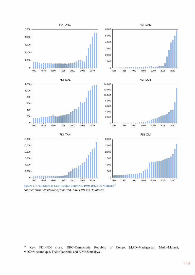
114
Figure 27: FDI Stock in Low Income Countries 1980-2012 (US Millions)44
Source: Own calculations from UNCTAD (2013a) Databases
44 Key: FDI=FDI stock, DRC=Democratic Republic of Congo, MAD=Madagascar, MAL=Malawi,
MOZ=Mozambique, TAN=Tanzania and ZIM=Zimbabwe.
0
1,000
2,000
3,000
4,000
5,000
1980 1985 1990 1995 2000 2005 2010
FDI_DRC
0
1,000
2,000
3,000
4,000
5,000
6,000
1980 1985 1990 1995 2000 2005 2010
FDI_MAD
0
200
400
600
800
1,000
1,200
1980 1985 1990 1995 2000 2005 2010
FDI_MAL
0
2,000
4,000
6,000
8,000
10,000
12,000
14,000
1980 1985 1990 1995 2000 2005 2010
FDI_MOZ
0
2,000
4,000
6,000
8,000
10,000
12,000
1980 1985 1990 1995 2000 2005 2010
FDI_TAN
0
500
1,000
1,500
2,000
2,500
3,000
1980 1985 1990 1995 2000 2005 2010
FDI_ZIM

115
Figure 28: Real GDP in Low Income Countries 1980-2012 (US Millions)45 Source: Own calculations from UNCTAD (2013a) Databases
In the empirical analysis, both variables are used in the logarithmic form, and the causality investigations
are conducted using log-differences (Ghali, 1988; Hurlin and Venet, 2008).
45 Key: GDP=Real GDP, DRC=Democratic Republic of Congo, MAD=Madagascar, MAL=Malawi,
MOZ=Mozambique, TAN=Tanzania and ZIM=Zimbabwe.
5,000
6,000
7,000
8,000
9,000
10,000
11,000
12,000
1980 1985 1990 1995 2000 2005 2010
GDP_DRC
3,000
3,500
4,000
4,500
5,000
5,500
6,000
6,500
1980 1985 1990 1995 2000 2005 2010
GDP_MAD
1,000
2,000
3,000
4,000
5,000
1980 1985 1990 1995 2000 2005 2010
GDP_MAL
0
2,000
4,000
6,000
8,000
10,000
12,000
1980 1985 1990 1995 2000 2005 2010
GDP_MOZ
4,000
8,000
12,000
16,000
20,000
24,000
1980 1985 1990 1995 2000 2005 2010
GDP_TAN
4,000
5,000
6,000
7,000
8,000
9,000
1980 1985 1990 1995 2000 2005 2010
GDP_ZIM
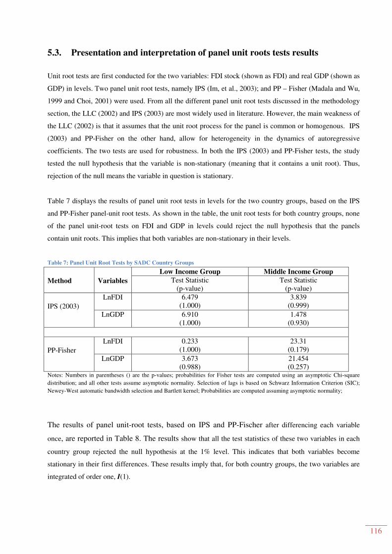
116
5.3. Presentation and interpretation of panel unit roots tests results
Unit root tests are first conducted for the two variables: FDI stock (shown as FDI) and real GDP (shown as
GDP) in levels. Two panel unit root tests, namely IPS (Im, et al., 2003); and PP – Fisher (Madala and Wu,
1999 and Choi, 2001) were used. From all the different panel unit root tests discussed in the methodology
section, the LLC (2002) and IPS (2003) are most widely used in literature. However, the main weakness of
the LLC (2002) is that it assumes that the unit root process for the panel is common or homogenous. IPS
(2003) and PP-Fisher on the other hand, allow for heterogeneity in the dynamics of autoregressive
coefficients. The two tests are used for robustness. In both the IPS (2003) and PP-Fisher tests, the study
tested the null hypothesis that the variable is non-stationary (meaning that it contains a unit root). Thus,
rejection of the null means the variable in question is stationary.
Table 7 displays the results of panel unit root tests in levels for the two country groups, based on the IPS
and PP-Fisher panel-unit root tests. As shown in the table, the unit root tests for both country groups, none
of the panel unit-root tests on FDI and GDP in levels could reject the null hypothesis that the panels
contain unit roots. This implies that both variables are non-stationary in their levels.
Table 7: Panel Unit Root Tests by SADC Country Groups
Method
Variables
Low Income Group Middle Income Group Test Statistic
(p-value) Test Statistic
(p-value) IPS (2003)
LnFDI 6.479 (1.000)
3.839 (0.999)
LnGDP 6.910 (1.000)
1.478 (0.930)
PP-Fisher
LnFDI 0.233 (1.000)
23.31 (0.179)
LnGDP 3.673 (0.988)
21.454 (0.257)
Notes: Numbers in parentheses () are the p-values; probabilities for Fisher tests are computed using an asymptotic Chi-square
distribution; and all other tests assume asymptotic normality. Selection of lags is based on Schwarz Information Criterion (SIC);
Newey-West automatic bandwidth selection and Bartlett kernel; Probabilities are computed assuming asymptotic normality;
The results of panel unit-root tests, based on IPS and PP-Fischer after differencing each variable
once, are reported in Table 8. The results show that all the test statistics of these two variables in each
country group rejected the null hypothesis at the 1% level. This indicates that both variables become
stationary in their first differences. These results imply that, for both country groups, the two variables are
integrated of order one, I(1).

117
Table 8: Panel Unit Root Tests by SADC Country Groups (First Difference)
Method
Variables
Low Income Group Middle Income Group Test Statistic
(p-value) Test Statistic
(p-value) IPS (2003)
∆LnFDI -8.355*** (0.000)
-10.69*** (0.000)
∆LnGDP -6.719*** (0.000)
-6.884*** (0.000)
PP-Fisher
∆LnFDI 83.915*** (0.000)
167.44*** (0.000)
∆LnGDP 80.087*** (0.000)
119.239*** (0.000)
Notes: Numbers in parentheses () are the p-values; probabilities for Fisher tests are computed using an asymptotic Chi-square
distribution; and all other tests assume asymptotic normality. Selection of lags is based on Schwarz Information Criterion (SIC);
Newey-West automatic bandwidth selection and Bartlett kernel; Probabilities are computed assuming asymptotic normality; ***
Rejects the null at the 1% level.
Based on the panel unit-root results, we proceed to test for cointegration between the two variables, for the
two country groups.
5.4. Panel cointegration test results
Panel cointegration tests investigate the presence of a long-run relationship between the two variables. This
is a test of whether there is a long-run relationship (Ghali, 1998; Basu, et al., 2003 and Lund, 2010:30).
Cointegration tests were conducted using the Pedroni (1999 and 2004) and Kao (1999) tests. The Pedroni
(1999 and 2004) tests heterogeneous panels. Pedroni’s cointegration tests amount to seven in total; and
they can be grouped into two: the ‘panel statistics’ or ‘within dimension’, which are equivalent to the unit-
root statistic against homogenous alternatives (Breitung and Pesaran, 2008); and the ‘group mean statistics’
or ‘between dimension’, which involve the averaging of the individually estimated AR coefficients for
each country, individually. All the seven Pedroni tests test the null hypothesis of no cointegration. The
Pedroni (1999 and 2004) statistics are one-sided tests with a critical value of -1.64. This means that a test
statistic of less than -1.64 (k < -1.64) implies rejection of the null for all other tests except the v-statistic.
For the panel-v, the critical value is 1.64. Thus a test statistic greater than 1.64 (k > 1.64) suggests rejection
of the null hypothesis of no cointegration. Lund (2010) also noted that when there is a conflict in the
results, the panel ADF and group ADF should be used. Table 9 shows the Pedroni panel and group results
for both low-income and middle-income groups.

118
Table 9: Pedroni Panel Cointegration Tests for FDI and GDP for SADC countries groups
Method
Low Income Group Middle Income Group Test Statistic
(p-value) Test Statistic
(p-value) Within Dimension / Panel Statistic
Panel v-Statistic (+) -0.709 (0.761)
1.681** (0.046)
Panel rho-Statistic 1.584 (0.943)
-1.769** (0.038)
Panel PP-Statistic 2.020 (0.978)
-2.386*** (0.009)
Panel ADF-Statistic 1.442 (0.925)
-2.362*** (0.009)
Between Dimensions / Group Mean Statistic
Group rho-Statistic 1.523 (0.936)
-0.851 (0.197)
Group PP-Statistic 2.045 (0.98)
-2.242** (0.013)
Group ADF-Statistic 1.770 (0.962)
-2.085** (0.019)
Notes: All statistics are from Pedroni’s procedure (1999) where the adjusted values can be compared to the N(0,1) distribution. The
Pedroni (2004) statistics are one-sided tests with a critical value of -1.64 (k < -1.64 implies rejection of the null), except the v-
statistic that has a critical value of 1.64 (k > 1.64 suggests rejection of the null). Numbers in parentheses () are the p-values;
Selection of lags is based on Schwarz Information Criterion (SIC); Newey-West automatic bandwidth selection and Bartlett kernel;
Probabilities are computed assuming asymptotic normality; *** Rejects the null at the 1% level; ** Rejects the null at the 5%
level; * Rejects the null at the 1% level. �+� the first test is a right-tail test while the other tests are left-tail tests; for consistence
we used un-weighted test statistics.
For the low-income country group, none of the four within-dimension panel-cointegration tests reject the
null hypothesis that there is no cointegration between FDI and GDP. Furthermore, none of the three group
tests could reject the null hypothesis. Overall, the seven Pedroni (1999 and 2004) tests show evidence of no
cointegration between the two variables for the low-income country group. The Kao (1999) panel
cointegration test was also conducted, for robustness; and it did not reject the null hypothesis of no
cointegration (See Table 10) for the low-income country group. Thus, both the Pedroni and Kao
cointegration tests fail to support the existence of any long-run relationship between FDI and economic
growth in low-income SADC countries.
This result was not expected, given that both theory and the empirical literature support the existence of a
long-run relationship between these two variables. Most seminal studies found evidence of the existence of
a long-run relationship between the FDI and economic growth (Ghali, 1998; Zhang, 2001; Lund, 2010 and
Fowowe, 2011). In some studies cointegration was found in certain countries (see Urbain, 1992; Zhang,
2001a and Moudatsou and Kyrkilis, 2011).
On the other hand, the four within-dimension panel cointegration tests for the middle-income country
group rejects the null hypothesis that there is no cointegration between the FDI and the GDP at a minimum
of 5% level of significance. Only one of the group tests could not reject the null hypothesis (See Table 9).
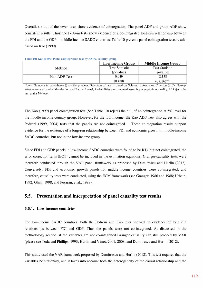
119
Overall, six out of the seven tests show evidence of cointegration. The panel ADF and group ADF show
consistent results. Thus, the Pedroni tests show evidence of a co-integrated long-run relationship between
the FDI and the GDP in middle-income SADC countries. Table 10 presents panel cointegration tests results
based on Kao (1999).
Table 10: Kao (1999) Panel cointegration test by SADC country group
Method
Low Income Group Middle Income Group Test Statistic
(p-value) Test Statistic
(p-value) Kao ADF Test 0.049
(0.480) -2.138
(0.016)** Notes: Numbers in parentheses () are the p-values; Selection of lags is based on Schwarz Information Criterion (SIC); Newey-
West automatic bandwidth selection and Bartlett kernel; Probabilities are computed assuming asymptotic normality; ** Rejects the
null at the 5% level.
The Kao (1999) panel cointegration test (See Table 10) rejects the null of no cointegration at 5% level for
the middle income country group. However, for the low income, the Kao ADF Test also agrees with the
Pedroni (1999, 2004) tests that the panels are not cointegrated. These cointegration results support
evidence for the existence of a long-run relationship between FDI and economic growth in middle-income
SADC countries, but not in the low-income group.
Since FDI and GDP panels in low-income SADC countries were found to be I(1), but not cointegrated, the
error correction term (ECT) cannot be included in the estimation equations. Granger-causality tests were
therefore conducted through the VAR panel framework as proposed by Dumitrescu and Hurlin (2012).
Conversely, FDI and economic growth panels for middle-income countries were co-integrated; and
therefore, causality tests were conducted, using the ECM framework (see Granger, 1986 and 1988; Urbain,
1992; Ghali, 1998; and Pesaran, et al., 1999).
5.5. Presentation and interpretation of panel causality test results
5.5.1. Low income countries
For low-income SADC countries, both the Pedroni and Kao tests showed no evidence of long run
relationships between FDI and GDP. Thus the panels were not co-integrated. As discussed in the
methodology section, if the variables are not co-integrated Granger causality can still proceed by VAR
(please see Toda and Phillips, 1993; Hurlin and Venet, 2001, 2008, and Dumitrescu and Hurlin, 2012).
This study used the VAR framework proposed by Dumitrescu and Hurlin (2012). This test requires that the
variables be stationary, and it takes into account both the heterogeneity of the causal relationship and the
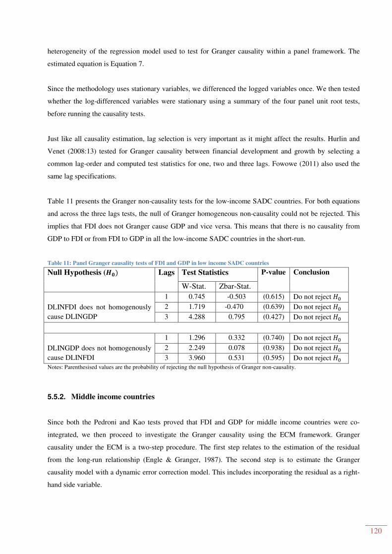
120
heterogeneity of the regression model used to test for Granger causality within a panel framework. The
estimated equation is Equation 7.
Since the methodology uses stationary variables, we differenced the logged variables once. We then tested
whether the log-differenced variables were stationary using a summary of the four panel unit root tests,
before running the causality tests.
Just like all causality estimation, lag selection is very important as it might affect the results. Hurlin and
Venet (2008:13) tested for Granger causality between financial development and growth by selecting a
common lag-order and computed test statistics for one, two and three lags. Fowowe (2011) also used the
same lag specifications.
Table 11 presents the Granger non-causality tests for the low-income SADC countries. For both equations
and across the three lags tests, the null of Granger homogeneous non-causality could not be rejected. This
implies that FDI does not Granger cause GDP and vice versa. This means that there is no causality from
GDP to FDI or from FDI to GDP in all the low-income SADC countries in the short-run.
Table 11: Panel Granger causality tests of FDI and GDP in low income SADC countries
Null Hypothesis (��� Lags Test Statistics P-value Conclusion
W-Stat. Zbar-Stat.
DLINFDI does not homogenously
cause DLINGDP
1 0.745 -0.503 (0.615) Do not reject -�
2 1.719 -0.470 (0.639) Do not reject -�
3 4.288 0.795 (0.427) Do not reject -�
DLINGDP does not homogenously
cause DLINFDI
1 1.296 0.332 (0.740) Do not reject -�
2 2.249 0.078 (0.938) Do not reject -�
3 3.960 0.531 (0.595) Do not reject -� Notes: Parenthesised values are the probability of rejecting the null hypothesis of Granger non-causality.
5.5.2. Middle income countries
Since both the Pedroni and Kao tests proved that FDI and GDP for middle income countries were co-
integrated, we then proceed to investigate the Granger causality using the ECM framework. Granger
causality under the ECM is a two-step procedure. The first step relates to the estimation of the residual
from the long-run relationship (Engle & Granger, 1987). The second step is to estimate the Granger
causality model with a dynamic error correction model. This includes incorporating the residual as a right-
hand side variable.

121
The panel Granger causality model with dynamic error correction was estimated in the form of the two co-
integrated equations (Equation 8 and 9). The ECM approach helps investigate the short and long run
Granger causality between FDI and GDP. In summary, the analysis and interpretation of causality results
under the ECM framework is as follows:
• Long-run causality is tested based on the statistical significance of the coefficient of the error
correction terms (7�� and 7"�) in Equation 8 and 9 respectively. Separate t-tests on the
coefficients of each of the error terms are applied.
• Short-run causality is tested on the coefficients of one of the explanatory variables. A Wald (1943)
F-test statistic is applied, which is a test of the joint significance of the other variable(s) in a
regression that includes lags of the dependent variable.
The estimated results of Equation 8 and 9 are presented in Table 12 below46. The results of Equation 8 are
in the row where ∆������ is the dependant variable while Equation 9 is the next row.
Table 12: Panel Granger causality tests results for middle income countries
Dependent
Variable
Source of causation (independent variable)
Short-run Long-run
∆��2��� ∆��2#�$ 89:
∆������ - 3.155*
(0.077)
-0.060
[-3.889] ***
∆��� �¡ [0.013]
(0.910)
- -0.00055
[-0.250]
Notes: Short Run- Figures denote F-statistic values and p-values in brackets (). For the long-run coefficient of the ECT are
reported, the square brackets [] are t-statistics. . Significance at the 1% and 10% is denoted by *** and * respectively.
With respect to Equation 8 (the FDI equation), the corresponding F-statistic for the GDP variable is
statistically significant at 10%. This implies that economic growth Granger causes FDI in the transitory
period (the short-run). As expected, the coefficient of the error correction term (ECT) on the FDI equation
is negative and statistically significant at 5% level. This implies that GDP Granger causes FDI in the long-
run.
The result on the GDP equation on the other hand shows that the corresponding F-statistic for the FDI
variable is statistically insignificant. This means that FDI does not Granger cause GDP in the short-run. For
the long-run causality, the coefficient of ECT is negative (as expected) but insignificant, thus implying that
FDI does not Granger cause GDP in both the short- and long-run. Overall, causality for the SADC middle
income countries is uni-directional, running from GDP to FDI.
46 The ECMs were run with different lags from 2 to 9 to see if the results were sensitive to changes but nothing
qualitative changed. Lag 5 was chosen as it had a high Adjusted R-squared and results are consistent with economic
literature.
122
On the direction of causality, Moudatsou and Kyrkilis (2011) used a similar methodology for the EU and
ASEAN economic associations and found evidence of growth causing FDI in EU and two-way causality in
ASEAN. Another study by Lund (2010) separated the country groups into low, middle and high income
and found that (i) in low-income countries there was no short run causal relationship, while causality was
uni-directional from GDP to FDI in in the long-run; (ii) in middle-income countries, causality was uni-
directional from GDP to FDI in both periods; (iii) high-income countries showed evidence of bi-
directional causality in the short-run and uni-directional causality from GDP to FDI, and (iv) no evidence
of bi-directional in the long-run. Thus the direction of causality for lower to middle income countries
(including African countries) is mainly from growth to FDI.

123
CHAPTER 6: CONCLUSION AND POLICY IMPLICATIONS
6.1. Introduction
This chapter summaries and concludes the study. It also offers policy implications based on the main
results of the study. The main sections of this chapter as are follows: Section 6.2, which summarises the
entire study; Section 6.3 briefly discusses empirical findings of the study; Section 6.4 presents policy
implications and recommendations while Section 6.5 highlights limitations of the study and suggests areas
for further research.
6.2. Summary of the study
The main objective of this study was to examine the causal relationship between FDI inflows and
economic growth in SADC countries. The study also investigated whether Granger causality was
dependent on the country’s level of income. In order to meet these two broad objectives, the study
investigated the dynamics of FDI and GDP in SADC countries over the period 1980-2012; explored both
theoretical and empirical research on the causal relationship between FDI and economic growth; and used
the recently developed panel-data analysis methods to examine this causal relationship. This section offers
a summary of the main findings per chapter, except empirical findings which are discussed separately in
Section 6.3.
The study noted that global FDI inflows have grown from US$50 billion in the early 1980s to US$1.5
trillion by 2011, although they fell by 18 per cent to $1.35 trillion in 2012. Africa and the SADC have also
witnessed substantial increases in FDI inflows. For SADC, FDI inflows have grown by almost fifty times
the original investment in the last three decades; from a mere US$372 million in 1980 to US$17 billion in
2008. Although FDI inflows to SADC decreased to US$7 billion in 2010, there are signs of recovery, as
2011 recorded a 38% increase to US$10 billion.
In Chapter 2, the case study approach was employed to analyse the policies and strategies used by
individual countries to attract FDI and boost economic growth. The findings of this study show that in the
1980s and early 1990s most SADC countries were still coming out of colonialism; and hence their policies
were mainly focused on import substitution, socialism and command economies, with strong emphasis on
the protection of infant industries. In particular, the governments of some of these countries were very
active in the market through State-owned enterprises (SOEs), especially in ‘strategic sectors’, such as
telecommunication, agriculture and mining. Most of these policies had a somewhat negative effect on FDI
inflows which were thus fairly low during the first two decades. FDI into SADC started peaking in the late
1990s, as governments embarked on privatisation, liberalisation and economic structural-adjustment

124
programmes. These reforms saw the warming up of countries to MNCs, and the setting up of investment-
promotion agencies. Some of the policies that were implemented by these countries include: i) The
deregulation of the economy; ii) the relaxation of exchange controls; iii) the adoption of 'market-friendly'
policies, such as privatisation and trade liberalisation; iv) the protection of foreign investments; v) political
stability; and vi) participation in multilateral and bilateral trade and investment agreements. In recent years,
some of these countries introduced special economic zones that offer further incentives to investors in
‘strategic industries’ such as manufacturing, tourism and oil exploration. It is also worth noting that
countries, such as South Africa, Zambia etc., that pursued the privatisation of State-owned enterprises,
recorded a significant increase in FDI inflows and economic growth.
Notwithstanding a remarkable increase in FDI inflows in recent years in these countries, there were still a
number of challenges faced by some of these countries which include, inter alia, civil wars, social unrest
and political strife which ravaged some of these economies during the 1990s and the early 2000s. Some of
the constraints currently facing FDI inflows into these SADC countries include political instability
(including civil wars), policy uncertainty, poor infrastructure, and difficulties in doing business.
Chapter 3 surveyed theoretical and empirical literature on the effect and causal relationship between FDI
and economic growth. The theoretical investigation showed that FDI is a key contributor to the economic
growth of the host country. Through both exogenous and endogenous growth analysis, it was noted that
FDI contributes directly and indirectly to economic growth, and that host country’s growth may attract
more FDI. It was also observed that FDI affects economic growth through two broad channels: (i) FDI can
encourage the adoption of new technologies in the production process through technological spillovers, and
(ii) FDI may stimulate knowledge transfers, both in terms of labour training and skill acquisition and by
introducing alternative management practices and better organisational arrangements; commonly referred
to as spillovers. It was also further noted that (i) the impact of FDI on economic growth can be positive or
negative, depending on channel or impact mechanism, and (ii) the impact of FDI on host country economic
growth is dependent on the economic and technological conditions in the host country itself, such as level
of human capital, the trading system, the degree of openness of the economy, investment policies and
legislation and political stability. A review of empirical literature showed that a causal relationship and link
between FDI and GDP could be in the form of growth-driven FDI (GDP causing FDI), FDI-led growth
(FDI causing GDP) and/or feedback (bi-directional causality).
Most of the studies proved that high economic growth rates were correlated with high investment rates, but
the results on causality were mixed and inconclusive. The majority of the studies showed evidence of
unidirectional causality from FDI to economic growth, while some found bi-directional causality.

125
Chapter 4 presents the recently developed panel data analysis methods, which include panel unit root tests,
panel cointegration tests and panel Granger causality tests. The chapter discussed two main methods of
performing Granger causality tests (i) the VAR model, which is applicable for stationary data where there
is no cointegration and (ii) the ECM for co-integrated variables. An argument is made that if the variables
are not co-integrated, Granger causality can still be tested using a VAR model and if co-integrated, an
ECM framework is used.
Empirical results are summarised below.
6.3. Summary and discussion of empirical findings
The empirical analysis involved examining the causal relationship between inward FDI and economic
growth and investigating whether causation was short-term, long-term or both. The study also explored
whether the causal relationship between the two variables varied according to income level. Furthermore,
the study also tested for (i) hypothesis of growth-driven FDI, (ii) hypothesis of FDI-led growth and (iii)
hypothesis of feedback; using SADC countries as a case study. The study used real GDP as a proxy for
economic growth and FDI stock as a proxy for FDI for the period 1980-2012.
The main findings of the study are summarised below:
i. Panel unit root (integration) tests showed that both variables were integrated of order one, I(1) for
both low and middle income SADC country groups.
ii. Panel cointegration was confirmed in middle-income countries, but not in the low-income
countries.
iii. Granger causality tests were then conducted using two different methodologies. For the low
income country group, a VAR proposed by Dumitrescu and Hurlin (2012) was employed, while an
ECM based Granger causality model was used for the middle income group.
iv. Granger causality tests results for the low-income countries’ panel show that there was no evidence
of causality in either direction – either in the short run, or in the long run.
v. For the middle-income countries’ panel, Granger causality tests results showed that there was a
unidirectional causal flow from GDP to FDI in both the long run and short run.
The results of this study support the Growth-led FDI hypothesis, but not the FDI-led growth hypothesis. In
other words, it is economic growth that drives FDI inflows into the SADC region, and not vice versa.
These results imply that the recent high economic growth rates that have been recorded in some of the
SADC countries, especially the middle-income countries, have led to a massive inflow of foreign direct
investment into this region. The cointegration tests confirm the long run relationship between FDI and
economic growth, and Granger causality tests showed that GDP causes FDI in middle income SADC

126
countries. This is in line with the new growth theories which suggest that GDP can attract FDI, especially
those MNCs which are markets and profits seeking. Economic growth can potentially release resources for
new infrastructure, improvement in human capital and also act as an increase in aggregate demand, which
attracts FDI. On the other hand, FDI in turn leads to an increase in GDP through increase in capital, new
technology, improvement in skills and other positive spillovers. This might lead to a positive feedback
between FDI and economic growth.
6.4. Policy implications and recommendations
The growth-driven FDI hypothesis was confirmed, especially in middle-income SADC countries. There
was causation in the short run for both middle and low income countries. This result comes against the
background that SADC as an institution, and individual countries have been very active in pursuing
policies and strategies in attracting FDI. Most policy makers have been advocating for more FDIs as one of
the strategies to boost national, regional and international economies.
The result of this study confirms an age-old debate that FDI into African countries has not resulted in
growth, mainly because investors have always repatriated their monies back. Secondly, the direct benefit of
FDI has been tax revenue, which does not seem to benefit the economy owing to corruption and economic
mismanagement.
Though it is recommended that SADC countries continue to deepen and intensify policies aimed at
attracting FDI and stimulating economic growth, it is imperative that policy makers give attention to other
growth enhancing factors over and above the attraction of FDI. Lund (2010:49) remarked that “blindly
reducing restrictions on FDI will most likely not result in long-run growth”. To promote economic growth,
SADC countries might consider stimulating domestic investment in infrastructure, education, technology
and exports, as they may be better alternatives. Several studies have shown that only after the host country
has reached a certain level of development will FDI positively affect economic growth.
Furthermore, theories on MNCs reveal broadly that location of FDI is determined by the anticipated
profitability on specific projects, ease with which foreign affiliates’ operations could be amalgamated into
the MNC’s global policies, and the overall quality of the host country’s enabling environment. To attract
FDI and benefit fully from its positive spillovers; host country policy makers could work on promoting
political and economic stability, building of institutional frameworks; crafting of a regulatory environment
favorable to inward FDI, including foreign investment incentive schemes; build and upgrade infrastructure,
technology and human skills.

127
SADC as a region should continue to pursue regional integration initiatives through removal of cross-
border trade and investment barriers between countries. This would attract more market-seeking FDI and
in turn boost economic growth. Since the study found that it is a countries’ growth which attracts FDI
inflows, then the SADC countries are urged to pay increased attention to policies and strategies focused on
the overall role and the quality of growth as a vital determinant of FDI.
6.5. Limitations of the study and suggestions for further research
The Granger causality analysis employed in this study only investigates the direction of causality and
whether each variable can be used to explain another, but does not directly test for the mechanisms through
which FDI leads to economic growth and economic growth leads to FDI. A more complete analysis, which
seeks to explain the channels through which FDI impacts growth is suggested for future studies.
Methodology applied in this study is a bivariate framework, which is likely to suffer from the omission of
variable bias (see Loizides and Vamvoukas, 2005; and Odhiambo, 2008 and 2011). Future studies may
include a third variable such as domestic savings, exports, or financial development in a trivariate or
multivariate panel causality model.
It is also suggested that future research be conducted at sector level and on a country by country basis. As
indicated in the review of literature, the effect of FDI on growth is heterogeneous across country and
sector. Sector level analysis will help policy makers draft effective industrial policies, which can guide
allocation of incentives.
The study did not show results by levels of individual countries’ development. Future studies may also
consider subdividing SADC countries into middle and lower income countries and then test for causality
separately.

128
BIBLIOGRAPHY
Abaidoo, R. 2012. Economic growth, regional savings and FDI in Sub-Saharan Africa: Trivariate causality
and error correction modeling approach. International Journal of Economics and Finance; Vol. 4, No. 11.
Acaravci, A. & Ozturk,I. 2012. Foreign direct investment, export and economic growth: Empirical
evidence from new EU countries. Romanian Journal of Economic Forecasting, 2: 52-67.
ADB (African Development Bank). 2009a. Botswana country strategy paper 2009 – 2013. Tunis-
Belvedère: African Development Bank.
ADB. 2009b. Regional economic development in Bas Congo in the context of decentralization in the
Democratic Republic of Congo (DRC). Available at:
http://www.afdb.org/fileadmin/uploads/afdb/Documents/Project-and-
Operations/DRC_Etude%20decentralisation_english__01.pdf (accessed on June 4, 2013).
ADB. 2011a. Angola country strategy paper 2011 – 2015. Tunis-Belvedère: African Development Bank.
ADB. 2011b. Seychelles country strategy paper 2011-2015. Tunis-Belvedère: African Development Bank.
ADB. 2012a. African economic outlook 2012. 2nd Quarter 2011, Issue No.1. Tunis-Belvedère: African
Development Bank.
ADB. 2012b. Angola 2012-Africa economic outlook. AfDB, OECD, UNDP, UNECA. Available at:
www.africaneconomicoutlook.org/en (accessed on June 04, 2013).
Agrawal, G. 2013. Foreign direct investment & economic growth in BRICS economies: A panel data
analysis. Paper presented at the 23rd International Business Research Conference 18 - 20 November, 2013,
Marriott Hotel, Melbourne, Australia.
Aitken, B.J. & Harrison, A. 1999. Do domestic firms benefit from direct foreign investment? Evidence
from Venezuela. American Economic Review 89:605–618.
Akinlo, A.E. 2004. Foreign direct investment and growth in Nigeria: An empirical investigation. Journal of
Policy Modelling, 26: 627-639.
Al Nasser, O.M. 2010. How does foreign direct investment affect economic growth? The role of local
conditions. Latin American Business Review, 11: 111-139.
Alfaro, L. 2003. Foreign direct investment and growth: Does the sector matter? Harvard Business School,
Working Paper. Available at:
http://gwww.grips.ac.jp/teacher/oono/hp/docu01/paper14.pdf (Accessed on 25/10/2013).
Alfaro, L., Chanda, A., Kalemli-Ozcan, S. & Sayek, S. 2003. FDI and economic growth: The role of local
financial markets. Available at: http://econweb.umd.edu/~kalemli/jiefinal.pdf (Accessed on
25/10/2013).

129
Alfaro, L., Chanda, A., Kalemli-Ozcan, S. & Sayek, S. 2004. FDI and economic growth: The role of local
financial Markets. Journal of International Economics, 64(1): 89-112.
Alves, A. C. 2012. Chinese economic and trade co-operation zones in Africa: Facing the challenges. Policy
Briefing 51. South African Institute of International Affairs (SAIIA).
ANIP (National Private Investment Agency). 2013. Available at: http://www.anip.co.ao/ (accessed on June
4, 2013).
ANAPI (National Agency for Investment Promotion). 2006. Reasons to Invest in DRC. Available at:
http://www.anapi.org/spip.php?page=article_en&id_article=302 (accessed on June 4, 2013).
Apergis, N. & Payne, J.E. 2010. Energy consumption and growth in South America: Evidence from a panel
error correction model. Energy Economics 32: 1421–1426.
Arvanitis, A. 2005. Foreign direct investment in South Africa: why has it been so low? Post-apartheid
South Africa: first ten years. Washington, DC: International Monetary Fund (IMF).
Asafa-Adjei, A. 2007. Foreign direct investments and its importance to the economy of South Africa.
Masters dissertation, University of South Africa. Pretoria.
Asheghian, P. 2011. Economic growth determinants and foreign direct investment causality in Canada.
International Journal of Business and Social Science, Vol. 2 No. 11.
AU (African Union). 2001. The New Partnership for Africa’s Development (NEPAD). Abuja: African
Union.
Balasubramanyam, V.N., Salisu, M. & Sapsford, D. 1996. Foreign direct investment and growth in EP and
IS countries. The Economic Journal, 106: 92-105.
Balasubramanyam, V.N., Salisu, M. & Sapsford, D. 1999. Foreign direct investment as an engine of
growth. The Journal of International Trade and Economic Development, 8(1): 92-105.
Baltagi, B. H. 2008. Econometric analysis of panel data. Fourth Edition. West Sussex: John Wely and
Sons, Ltd.
Bank of Botswana. 2012. Annual Report 2012. Gaborone: Bank of Botswana.
Bank of Tanzania. 2012. Monetary Policy Statement. Dar es Salaam: Bank of Tanzania.
Barro, R. and Sala-I-Martin, X. 1995. Economic Growth. Cambridge, MA: McGraw-Hill.
Basdevant, O., Baba, C. & Mircheva, B. 2011. Macroeconomic vulnerabilities stemming from the global
economic crisis: The case of Swaziland. Washington, D.C.: International Monetary Fund (IMF).
Basu, P., Chakraborty, C. & Reagle, D. 2003. Liberalisation, FDI, and growth in developing countries: A
panel cointegration approach. Economic Inquiry 41 (3): 510-516.

130
Batten, J.A. & Vo, X.V. 2009. An analysis of the relationship between foreign direct investment and
economic growth. Applied Economics, 41:1621–1641.
BEDIA (Botswana Export Development and Investment Authority). 2013. Botswana Export Development
and Investment Authority. Available at: http://www.bedia.co.bw/. (Accessed on July 10, 2013).
Berthélemy, J.C. & Démurger, S. 2000. Foreign direct investment and economic growth: Theory and
application to China. Review of Development Economics, 4 (2): 140 – 155.
Borensztein, E., Gregorio, J. & Lee, J.W. 1998. How does foreign direct investment affect economic
growth? Journal of International Economics, 45: 115-135.
Boyd, J. H., & Smith, B. D. 1992. Intermediation and the equilibrium allocation of investment capital:
Implications for economic development. Journal of Monetary Economics, 30(3): 409-32.
Breitung, J. 2000. The local power of some unit root tests for panel data. Advances in Econometrics
15:161-177.
Breitung, J. & Pesaran, M. H. 2008. Unit root and cointegration in panels, in the econometrics of panel
data: Fundamentals and recent developments in theory and practice, third edition, edited by L. Mátyás &
P. Sevestre. Berlin Heidelberg: Springer-Verlag.
Brouthers, L.E., Gao,Y. & Mcnicol, J.P. 2008. Research notes and commentaries corruption and market
attractiveness influences on different types of FDI. Strategic Management Journal, Vol.29, pp.673-680.
Buckley, J.P., Jeremy, C., & Chengqi, W. 2002. The impact of inward FDI on the performance of China’s
manufacturing firms. Journal of International Business Studies, 33(4): 637-655.
Canning, D. & Pedroni, P. Infrastructure, long-run economic growth and causality tests for co-integrated
panels. The Manchester School 76 (5): 504–527.
Cao, X. & Jariyapan, P. 2012. Foreign direct investment, human capital and economic growth of People’s
Republic of China using panel data approach. CMU, Journal of Economics.
Carbaugh, R. J. 2008. International economics. 11th Edition. , New Delhi: Thomson South-Western.
Cardoso, F. H. & Faletto, E. 1970. Dependency & development in Latin America. Berkeley, CA:
University of California Press.
Carkovic, M. & Levine, R. 2003. Does foreign direct investment accelerate economic growth? University
of Minnesota, Working Paper. Available at:
http://siteresources.worldbank.org/INTFR/Resources/fdi.pdf (Accessed on October 25, 2013).
Caves, R.E. 1996. Multinational enterprise and economic analysis. Cambridge: Cambridge University
Press.
Central Bank of Seychelles. 2012. Annual Report 2012. Victoria: Central Bank of Seychelles.

131
Chakraborty, C. & Basu, P. 2002. Foreign direct investment and growth in India: A cointegration
approach. Applied Economics, 34, 1061-1073.
Chakrabotry, C. & Nunenkamp, P. 2006. Economic reforms, foreign direct investment
and its economic effects in India. Working Paper No. 1272, Kiel Institute for the World Economy.
Chirwa, E. W. & Zakeyo, C. 2003. Impact of economic and trade policy reforms on food security in
Malawi. Report submitted to the Food and Agriculture Organisation (FAO) and the African Economic
Research Consortium (AERC).
Chirwa, E. W. 2005. Macroeconomic policies and poverty reduction in Malawi: Can we infer from panel
data? Report submitted to Global Development Network (GDN), Washington, DC.
Choe, J. I. 2003. Do foreign direct investment and gross domestic investment promote economic growth?
Review of Development Economics, 7 (1): 44–57.
Choi, I. 2001. Unit root tests for panel data. Journal of International Money and Finance 20: 249–272.
Chowdhury, A. & Mavrotas, G. 2003. FDI and growth: What causes what?, WIDER Conference on
“Sharing global prosperity”, WIDER, Helsínquia, Setembro 1 to 18.
Chowdhury, A. & Mavrotas, G. 2005. FDI and growth: A causal relationship. United Nations University.
World Institute for Development Economic Research, Research Paper No. 2005/25.
Chowdhury, A. & Mavrotas, G. 2006. FDI and growth: What causes what? United Nations University, The
World Economy.
Clark, D.P., Highfill, J., Jonas de Oliveira Campino, J.O., and Rehman, S.S. 2011. FDI, technology
spillovers, growth, and income inequality: A selective survey. Global Economy Journal, 11 (2):1-42.
Cobb C. W. and Douglas P. H. 1928. A theory of production. The American Economic Review, Vol.
XVIII.
Collier, P., Dollar, D. & World Bank. 2002. The new wave of globalisation and its economic effects. In
Globalisation, growth, and poverty: building an inclusive world economy. A World Bank policy research
report. Washnington D.C.: World Bank.
COMESA (Common Market for Eastern and Southern Africa). 2012. Regional integration and foreign
direct investment in COMESA. COMESA Investment Report 2012. Lusaka: COMESA.
Cousins, B. 2003. The Zimbabwean crisis in its wider context: the politics of land, democracy and
development in southern Africa, in Hammar, A, Raftopoulos, B and S. Jansen (eds), Zimbabwe’s
unfinished business: rethinking land, state and nation in the context of crisis, Harare: Weaver Press, 2003,
pp: 263 – 316.
Crotty, J., Epsten, G. & Kelly, P. 1998. Multinational corporations in the neo-liberal regime, in
Globalisation and progressive economic policy, edited by D. Baker, G. Epstein, R. Pollin. Cambridge:
Cambridge UP.

132
Cunguara, B. 2011. Assessing strategies to reduce poverty in rural Mozambique. PhD thesis, Department
of Economics and Social Sciences, University of Natural Resources and Life Sciences. Vienna.
Davies, R. & Rattsø, J. 2000. Zimbabwe: Economic adjustment, income distribution and trade
liberalisation. Working Paper No. 21. Center for Economic Policy Analysis, New School University. New
York.
De Jager, J. L. W. 2004. Exogenous and Endogenous Growth, University of Pretoria ETD.
De Mello, L.R. 1997. Foreign direct investment in developing countries: a selective survey. Journal of
Development Studies, 34(1):1–34.
De Mello, L.R. 1999. Foreign direct investment – led growth: evidence from time series and panel data.
Oxford Economic Papers, 51: 133 – 151.
Dickey, D.A. and Fuller, W.A. 1979. Distributions of the estimators for autoregressive time series with a
unit root, Journal of the American Statistical Association 74: 427-31.
Dickey, D.A. and Fuller, W.A. 1981. Likelihood ratio statistics for autoregressive time series with a unit
root. Econometrica 49:1057-72.
Dorosh, P. 1994. Macroeconomic adjustment and the poor in Madagascar: A CGE analysis. Working
Paper, CFNPP Publications Department. Cornell University. New York.
Dumitrescu, E. and Hurlin, C. 2012. Testing for granger non-causality in heterogeneous panels. Economic
Modelling 29: 450–1460.
Dupasquier, C. & Osakwe, P.N. 2005. Foreign direct investment in Africa: Performance, challenges and
responsibilities, Journal of Asian Economics, Elsevier, 17(2), 241-260.
Duttaray, M., Dutt, A. & Mukhopadhyay, K. 2008. Foreign direct investment and economic growth in less
developed countries: An empirical study of causality and mechanisms. Applied Economics, 40: 1927 –
1939.
Dritsaki, M., Dritsaki, C. and Adamopoulos, A. 2004. A causal relationship between trade, foreign direct
investment and economic growth in Greece. American Journal of Applied Sciences 1 (3) 230-235.
Elboiashi, H. A. 2011. The effect of FDI and other foreign capital inflows on growth and investment in
developing economies. PhD thesis, Department of Economics, University of Glasgow.
Elboiashi, H. A., Noorbakhsh, F., Paloni, A. & Azemar, C. 2009. The causal relationship between foreign
direct investment, domestic investment and economic growth in North African non-oil producing
countries: Empirical evidence from cointegration analysis. Advances in Management, Vol. 2 (11): 19-25.
Emirmahmutoglu, F. & Kose, N. 2011. Testing for Granger causality in heterogeneous mixed panels.
Economic Modelling 28:870-876.

133
Engle, R. F. & Granger C. W. J. 1987. Cointegration and error correction: Representation, estimation, and
testing. Econometrica 55(2): 251-276.
Eragha, P.B. 2011. The dynamic linkages between foreign direct investment and domestic investment in
ECOWAS countries: A panel cointegration analysis. Paper Presented at the 2011 Conference of the Centre
for the Study of African Economies, Oxford University, Oxford, UK between 20th-22nd March.
Erdil, E. and Yetkiner, I. H. 2006. A panel data approach for income-health causality, Working Papers
FNU-47, Research unit Sustainability and Global Change, Hamburg University.
Esso, L. J. 2010. Long-run relationship and causality between foreign direct investment and growth:
evidence from ten African countries. International Journal of Economics and Finance Vol. 2, No. 2; pp:
168-177.
Evans, P. 1979. Dependent development: The alliance of multinational, state, and local capital in Brazil.
Princeton: Princeton UP.
Faeth, I. 2009. Determinants of foreign direct investment – A tale of nine theoretical models. Journal of
Economic Surveys, 23(1): 165-196. Available at: http://dx.doi.org/10.1111/j.1467-6419.2008.00560.x
(Accessed on July 11, 2013).
fDi Intelligence. 2013. fDi Intelligence Website. Available at: http://www.fdiintelligence.com/ (accessed
June 20, 2013).
Feridun, M. and Sissoko, Y. 2011. Impact of FDI on economic development: A causality analysis for
Singapore, 1976 – 2002. International Journal of Economic Sciences and Applied Research 4 (1): 7-17.
FAO (Food and Agriculture Organisation of the United Nations). 2011. Foreign agricultural investment
country profile: Angola. Viale delle Terme di Caracalla, 00153. Rome: United Nations.
FAO. 2012. Foreign agricultural investment country profile: DRC. Rome: United Nations.
Ford, T., Rork, J. and Elmslie, B. 2008. Foreign direct investment, economic growth, and the
human capital threshold: Evidence from US states. Review of International Economics, 16 (1): 96
– 113.
Foster, V. & Benitez, D. A. 2011. The Democratic Republic of Congo’s infrastructure: A continental
perspective. Policy Research Working Paper No. 5602. Washington D.C.: The World Bank.
Fowowe, B. 2011. The finance-growth nexus in Sub-Saharan Africa: Panel cointegration and causality
tests. Journal of International Economics 23:220-239.
Fisher, R. A. 1932. Statistical methods for research workers, Oliver & Boyd, Edinburgh, 4th Edition.
Gelb, S. 2003. Inequality in South Africa: Nature, causes and responses, DFID Policy Initiative on
Addressing Inequality in Middle-income Countries. Johannesburg: The EDGE Institute. Available at:
http://www.southafrica.info (accessed on July 04, 2013).

134
Gelb, S. & Black, A. 2004. Foreign direct investment in South Africa in Estrin, S., & Meyer, K. E. (Eds),
Investment strategies in emerging markets, London Business School Centre for New and Emerging
Markets (CNEM), Cheltenham: Edward Elgar Press.
Gershenberg, I. 1987. The training and spreading of managerial know-how: A comparative analysis of
multinationals and other firms in Kenya. World Development 15 (7): 931-939.
Ghali, K. H. 1998. Public investment and private capital formation in a vector error-correction model of
growth. Applied Economics, 30: 837–844.
Glennie, J. 2011. The role of aid to middle-income countries: a contribution to evolving EU development
policy. Working Paper 331, Overseas Development Institute. London.
Government of Angola. 2011. New Private Investment Law (LAW No. 20/11). Luanda: Republic Angola
Government Gazette. Available at:
http://www.eisourcebook.org/cms/Angolan%20Basic%20Law%20for%20Private%20Investment.pdf
(accessed on June 04, 2013).
Government of Botswana. Ministry of Finance and Development Planning (MFDP). 1997. National
Development Plan 8 (1997/08-2002/03). Gaborone: Government printer.
Government of Botswana. Ministry of Finance and Development Planning (MFDP). 2003. National
Development Plan 9 (2003/04-2008/09). Gaborone: Government printer.
Government of Botswana. Ministry of Finance and Development Planning (MFDP). 2007. Macroeconomic
outline and policy framework for NDP 10. Gaborone: Government printer.
Government of Botswana. Ministry of Finance and Development Planning (MFDP). 2009. 2009 Budget
Speech. Turning challenges into opportunities-building on achievement of NDP 9. Gaborone: Government
printer.
Government of Lesotho. 2013. Private sector competitiveness and economic diversification project.
Available at: http://www.psc.org.ls/news/STRATEGIC_PLAN_ONE_STOP_SHOP.php (accessed on July
04, 2013).
Government of Lesotho and International Monetary Fund (IMF). 2012. National strategic development
plan 2012/13 – 2016/17: Growth and development strategic framework. IMF Country Report No. 12/102.
Washington, D.C: International Monetary Fund (IMF).
Government of Madagascar. 2006. Madagascar Action Plan 2007-2012: A bold and exciting plan for rapid
development. Antananarivo: Government of Madagascar.
Government of Madagascar. 2013. Madagascar: Investing and doing business in the Great Island, land of
opportunities. Cape Town: Consulate General of Madagascar. Available at:
http://www.madagascarconsulate.org.za/indexeng.html (accessible on June 4, 2013).
Government of Malawi. 2003. Malawi Vision 2020. Lilongwe: Government of Malawi: Available at:
http://www.sdnp.org.mw/malawi/vision-2020 (accessible on June 4, 2013).

135
Government of Malawi. 2004. Malawi Economic Growth Strategy (MEGS). Lilongwe: Government of
Malawi.
Government of Malawi. 2012. Malawi Economic Recovery Plan (MERP). Lilongwe: Government of
Malawi.
Government of Malawi and International Monetary Fund (IMF). (2012). Malawi Growth and Development
Strategy II 2011-2016. (IMF Country Report No. 12/222). Washington, D.C.: International Monetary
Fund.
Government of Namibia. 1998. Review of the 1992 white paper on industrial development. Windhoek:
Ministry of Trade and Industry (MTI).
Government of Namibia. 2004. Namibia vision 2030: policy framework for long-term national
development. Windhoek: Government of Namibia.
Government of Namibia. 2008. Third national development plan (NDP3) 2007/2008-2011/12. Windhoek:
Government of Namibia.
Government of Namibia. 2012. Namibia’s fourth national development plan (NDP4)2012/13 to 2016/17:
“changing gear towards vision 2030”. Windhoek: Government of Namibia.
Government of South Africa. The Presidency of South Africa. 2006. Accelerated and shared growth
initiative: A summary. Pretoria: The Presidency of South Africa.
Government of South Africa. The Presidency of South Africa. 2010. Framework of the new economic
growth path. Pretoria: The Presidency of South Africa. Available at:
http://www.info.gov.za/view/DownloadFileAction?id=135748 (accessed on July 24, 2013).
Government of South Africa. 2011. National development plan: Vision for 2030. Pretoria: National
Planning Commission.
Government of South Africa. 2013. South Africa: A trade, investment and tourism promotion guide-
2012/13 [Brochure, Issue 3]. Pretoria: QQP Publishers.
Government of Swaziland. 1999. National development strategy – vision 2022: Key macro and sectoral
strategies. Mbabane: Government of Swaziland.
Government of Swaziland and European Commission. 2002. Country strategy paper and national
indicative programme for the period 2001 – 2007. Mbabane: Government of Swaziland.
Government of Seychelles. 2007. Strategy 2017: Creating our nation’s wealth together. Victoria:
Government of Seychelles.
Government of Seychelles. Ministry of Education, Employment and Human Resources Employment
Department. 2010. Decent work country programme 2011 – 2015. Victoria: Ministry of Education,
Employment and Human Resources Employment Department.
136
Government of Tanzania. Ministry of Industry and Trade. 2003. National Trade Policy. Dar es Salaam:
Ministry of Industry and Trade.
Government of Zambia. Ministry of Finance and National Planning. 2004. Financial sector development
plan for Zambia 2004-2009. Lusaka: Ministry of Finance and National Planning.
Government of Zimbabwe. 1981. Growth with equity: An economic policy statement. Harare: Government
of Zimbabwe.
Government of Zimbabwe. 1991. Zimbabwe: A framework for economic reform 1991-95. Harare:
Government publication.
Government of Zimbabwe. 1996. Zimbabwe: Programme for economic and social transformation
(ZIMPREST), 1996- 2000. Harare: Jongwe Printers.
Government of Zimbabwe. 2009. Statement on the 2009 Budget. Harare: Ministry of Finance.
Government of Zimbabwe. 2011. Zimbabwe Medium Term Plan (2011-2015). Harare: Ministry of
Economic Planning and Investment Promotion.
Granger, C.W.J. 1969. Investigating causal relations by econometric models and cross-spectral
Methods. Econometrica 37 (3): 424–438.
Granger, C.W. J. 1986. Developments in the study of co-integrated economic variables. Oxford Bulletin of
Economics and Statistics, 48(3): 213-28.
Granger, C.W.J. 1988b. Some recent development in a concept of causality. Journal of Econometrics,
Elsevier, 39(1-2): 199-211.
Green, R. H. & Kadhani, X. 1986. Zimbabwe: Transition to economic crises 1981-1983: Retrospect and
prospect. World Development, 14 (8), 1059 -1083.
Greene W. H. 2012. Econometric analysis. Seventh edition, Harlow Essex: Pearson Education, Prentice
Hall.
GTZ (Deutsche Gesellschaft für Technische Zusammenarbeit). 2009. Foreign direct investment in land in
Madagascar. Report prepared on behalf of the Federal Ministry for Economic Cooperation and
Development. Eschborn: GTZ.
Gujarati, D. 2004. Basic Econometrics, Fourth Edition. The McGraw-Hill Companies.
Gwenhamo, F. 2009. Foreign direct investment in Zimbabwe: The role of institutional factors. Economics
Research Southern Africa (ERSA), Working Paper No. 144. Available at:
http://www.econrsa.org/system/files/publications/working_papers/wp144.pdf (accessible on June 4, 2013).
Hadri, K. 2000. Testing for stationarity in heterogeneous panel data. Econometrics Journal 3:148-161.

137
Hanke, H.S and Kwok, A.K.F. 2009. On the measurement of Zimbabwe’s hyperinflation. Cato Journal,
29(2):353-364.
Hanlon, J. (2010). Mozambique: the war ended 17 years ago, but we are still poor. Conflict, Security &
Development, 10(1), 77-102.
Hansen, H. and Rand, J. 2006. On the causal links between FDI and growth in developing countries. The
World Economy, Volume 29(1): 21–41.
Hermes, N. & Lensink, R. 2003. Foreign direct investment, financial development and economic growth.
Journal of Development Studies, 40(1):142-163.
Herzer, D., Klasen, S. and Nowak-Lehmann D. F. 2008. In search of FDI-led growth in developing
countries: the way forward. Economic Modelling 25(5): 793-810.
Hicks, J.R. 1932. Marginal productivity and the principle of variation. Economica 12: 79-88.
Ho, S., Kauffman, R. and Liang, T. 2007. A growth theory perspective on B2C e-commerce growth in
Europe: An exploratory study. Electronic Commerce Research and Applications 6: 237-259.
Holtz-Eakin, D., Newey, W. and Rosen, H.S. 1998. Estimating vector autoregressions with panel data.
Econometrica 56:1371–95.
Hsiao, C. 1986. Analysis of Panel Data. Cambridge: Cambridge University Press
Hsiao, C. 1989. Modelling Ontario regional electricity system demand using a mixed fixed and random
coefficients approach. Regional Science and Urban Economics, 19: 565-87.
Hsiao, C. 2003. Analysis of panel data, Second Edition. New York: Cambridge University Press.
Hurlin, C. 2004. Testing granger causality in heterogeneous panel data models with fixed coefficients, DR
LEO 2004-05, Econometric Theory, en révision.
Hurlin, C. 2007. Testing for granger non-causality in heterogeneous panels. Available at:
http://www.univ-orleans.fr/deg/masters/ESA/CH/Causality_2007.pdf (Accessed 09 September
2013).
Hurlin, C. 2008. Testing for granger non-causality in heterogeneous panels, Working Papers halshs-
00224434_v1, HAL.
Hurlin, C. and Venet, B. 2001. Granger causality tests in panel data models with fixed coefficients,
Working Paper Eurisco 2001-09, Université Paris Dauphine.
Hurlin, C. and Venet, B. 2003. Granger causality tests in panel data models with fixed coefficients.
Mimeograph, Universitie Paris I.
Hurlin, C. & Venet, B. 2008. Testing for Granger non causality in heterogeneous panel. Document de
Recherche LEO.
138
ILO (International Labour Organisation). 2010. Employment, poverty and economic development in
Madagascar: A macroeconomic framework. Employment Working Paper No. 58. Geneva: International
Labour Organisation.
Im, K.S., Pesaran, M.H. and Shin, Y. 2003. Testing for unit roots in heterogeneous panels. Journal of
Econometrics 115:53-74.
IMF (International Monetary Fund). 1993. Balance of payments manual. 5th ed. Washington, D.C.:
International Monetary Fund.
IMF. 2005. Zambia: Enhanced initiative for heavily indebted poor countries-completion point document.
IMF Country Report No. 05/137. Washington, D.C.: International Monetary Fund.
IMF. 2012. Regional economic outlook: Sub-Saharan Africa- Maintaining growth in an uncertain world.
Country Report No. 08/57. Washington, D.C.: International Monetary Fund.
IMF. 2013. Zimbabwe staff-monitored program. IMF Country Report No. 13/193. Washington, D.C.:
International Monetary Fund.
Jansson, J., Burke, C. & Jiang, W. 2009. Chinese companies in the extractive industries of Gabon & the
DRC: Perceptions of transparency. A research undertaking by the Centre for Chinese Studies, prepared for
the Extractive Industries Transparency Initiative (EITI) & Revenue Watch Institute (RWI). Cape Town:
Centre for Chinese Studies, University of Stellenbosch.
Jayachandran, G. and Seilan, A. 2010. A causal relationship between trade, foreign direct investment and
economic growth for India. International Research Journal of Finance and Economics, ISSN 1450-2887
Issue 42; pp: 75-88.
Jordaan, J. A. 2012. Empirical estimation of FDI spillovers: A critical survey, in Econometrics: New
research, edited by S. A. Mendez and A. M. Vega. New York: Nova Science Publishers, Inc.
Juma, M.A. 2012. The effect of foreign direct investment on growth in Sub-Saharan Africa. BA Honors
dissertation, Amherst College, Massachusetts, USA.
Kao, C. 1999. Spurious regression and residual-based tests for cointegration in panel data. Journal of
Econometrics 90 (1999):1-44.
Kavita, W & Sudhakara, R. 2011. Foreign direct investment into developing Asian countries: the role of
market seeking, resource seeking and efficiency seeking factors. International Journal of Business and
Management, 6(11):219-226.
Khawar, M. 2005. Foreign direct investment and economic growth: A cross-country analysis. Global
Economy Journal Vol. 5, No. 1, Article 8.
Kottaridi, C. 2005. The core-periphery pattern of FDI – led growth and production structure in the EU.
Applied Economics, 37: 99 – 113.

139
Kotrajaras, P., Tubtimtong, B. & Wiboonchutikula, P. 2011. Does FDI enhance economic growth? New
evidence from East Asia. ASEAN Economic Bulletin 28(20): 183–202.
Krugman, P & Obstfeld, M. 2008. International economics: Theory and policy. 8th edition. Addison
Wesley.
Lall, S. 2003. FDI, AGOA and manufactured exports from a land-locked, least developed African
economy: Lesotho. QEH Working Paper Series – QEHWPS109. Oxford: University of Oxford.
Lee, C. and Chang, C. 2009. FDI, financial development, and economic growth: International evidence.
Journal of Applied Economics. 12(2):249-271.
Levin, A., Lin, C. F. and Chu, C. S. J. 2002. Unit root tests in panel data: Asymptotic and finite-sample
properties. Journal of Econometrics 108:1–24.
Li, X and Liu, X. 2005. Foreign direct investment and economic growth: an increasingly endogenous
relationship. Word Development 33 (3): 393-407.
Liu, X., Shu, C. & Sinclair, P. 2009. Trade, foreign direct investment and economic growth in Asian
economies. Applied Economics, 41:1603–1612.
Lipsey, R.E. and Sjoholm, F. 2004. FDI and wage spillovers in Indonesia manufacturing. Review of World
Economics 140(2):287-310.
Liu, Z. 2008. Foreign direct investment and technology spillovers: Theory and evidence. Journal of
Development Economics 85: 176–193.
Lo, C., Lin, Y., Chi, T. and Joseph, D. J. 2013. Foreign direct investment inflows in Haiti: its determinants
and impact on economic growth. Business Management Dynamics 2 (9):36-50.
Loizides, J. and Vamvoukas, G. 2005. Government expenditure and economic growth: Evidence from tri-
variate causality testing. Journal of Applied Economics 8, 125-152
Lucas, R. 1988. On the mechanics of economic development. Journal of Monetary Economics, 22: 3-
42.
Lund, M.T. 2010. Foreign direct investment: Catalyst of economic growth? PhD thesis, University of Utah,
Salt Lake City.
Madala, G. S. and Wu, S. 1999. A comparative study of unit root tests with panel data and a new simple
test. Oxford Bulletin of Economics and Statistics, Special Issue, 631–652.
Madhoo, Y. N. and Nath, S. 2004. Explaining African economic growth performance: the case of
Mauritius. Draft Interim Report on Mauritius Case Study for the African Economic Research Consortium
Project “Explaining African Economic Growth Performance”. Nairobi: African Economic Research
Consortium.

140
Magalasi, C. 2009. The political economy of foreign direct investment in Malawi. Master of Business Law
Dissertation, Bucerius Law School and Otto Beisheim School of Management.
Magnus, F. J. and Fosu, O. E. 2008. Bivariate causality analysis between FDI inflows and economic
growth in Ghana. International Research Journal of Finance and Economics, 15:104-112.
Makki, S. and Somwaru, A. 2004. Impact of foreign direct investment and trade on economic growth:
evidence from developing countries. American Journal of Agricultural Economics, 86 (3): 795 – 801.
Majagaiya, K. P. and Gu, Q. 2010. A time series analysis of foreign direct investment and economic
growth: a case study of Nepal. International Journal of Business and Management, 5(2):144-148.
Malefane, M.R. 2007. Determinants of foreign direct investment in Lesotho: Evidence from cointegration
and error correction modelling. South African Journal of Economic and Management Sciences, 10(1), 99-
106.
Mankiw, N. G. 1995. The growth of nations. Brookings Papers on Economic Activity 1:275–326.
MacCoskey, S & Kao, C. 2001. A Monte Carlo comparison of tests for cointegration in panel data. Center
for Policy Research. Available at: http://web.syr.edu/`cdkao (accessible March 20, 2013).
Mehraral, M., Haghnejad, A., Jalal Dehnavi, J. & Meybodi, F.J. 2014. Dynamic causal relationships among
GDP, exports, and foreign direct investment (FDI) in the developing countries. International Letters of
Social and Humanistic Sciences, 3 (2014) 1-19.
MIGA (Multilateral Investment Guarantee Agency). 2006. Benchmarking FDI competitiveness:
Madagascar. Washington, DC: World Bank Group.
MIPA (Malawi Investment Promotion Agency). 2008. Trade and Investors. Lilongwe: MIPA.
Mencinger, J. 2003. Does Foreign Direct Investment Always Enhance Economic Growth?, Kilkos, 56 (4):
491 – 508.
Mohamed, M.R., Singh, K.S.J. & Liew, C. 2013. Impact of foreign direct investment & domestic
investment on economic growth of Malaysia. Malaysian Journal of Economic Studies 50(1):21-35.
Moran, T. 1978. Multinational corporations and dependency: A dialogue for dependentistas and non‐dependentistas. International Organization, 32:79‐100.
Moudatsou, A. 2001. Foreign direct investment and economic growth: Evidence from 14 European Union
Countries. Available at: http://www.iefs.org.uk/Papers/Moudatsou.pdf (accessed on May 03, 2013).
Moudatsou, A. & Kyrkilis, D. 2011. FDI and economic growth: Causality for the EU and ASEAN. Journal
of Economic Integration 26(3): 554-577.
Moura, R. and Forte, R. 2010. The effects of foreign direct investment on the host country economic
growth - theory and empirical evidence. FEP WORKING Papers, Research Work in Progress; No.
390, Faculdade de Economia, Universidade do Porto.

141
Mwanawina, I. 2007. Deepening integration in SADC: Zambia’s economic policies in line with SADC
targets. Regional Integration in Southern Africa Vol. 7. A study conducted for the Friedrich Ebert
Foundation. Gaborone: Friedrich Ebert Foundation.
Nair-Reichert, U. and Weinhold, D. 2001. Causality tests for cross-country panels: A look at FDI and
economic growth in Less Developed Countries. Oxford Bulletin of Economics and Statistics 63:153–171.
Ndlela, T. (2011). Evolution of Zimbabwe's economic tragedy: A chronological review of macroeconomic
policies and transition to the economic crisis. MPRA Paper No. 32703. Available at: http://mpra.ub.uni-
muenchen.de/32703/ (accessible on June 20, 2013).
Ncube, M., Shimeles, A. & Verdier-Chouchane, A. 2012. South Africa’s quest for inclusive development.
Working Paper No. 150. Tunis-Belvedère: African Development Bank Group.
Ndoricimpa, A. 2009. Foreign direct investments, exports and economic growth in COMESA countries: A
heterogeneous panel causality approach. Masters Dissertation, Master of Arts in Economics, Makerere
University.
Nord, R., Sobolev, Y., Dunn, D., Haldenberg, A., Hobdari, N., Maziad, S. & Ruudet, S. 2009. Tanzania-
the story of an African transition. Washington, D.C.: International Monetary Fund.
Nunnenkamp, P. & Spatz, J. 2003. Foreign direct investment and economic growth in developing
countries: How relevant are host-country and industry characteristics?. Kieler Arbeitspapiere, 1176, Institut
für Weltwirtschaft, Kiel, 45 pp.
OECD. 2002. Foreign direct investment for development: Maximising benefits, minimising costs. Paris:
OECD.
OECD. 2011. OECD investment policy review of Zambia: Advancing investment policy reform.
Preliminary Draft, Paris: OECD. Available at: http://www.oecd.org/daf/inv/investment-policy/zambia-
investmentpolicyreview-oecd (accessed on July 20, 2013).
Odada, J. E., and Godana, T. 2002. Sources of growth in Africa: A case study of Namibia. Working Paper,
Faculty of Economics and Management Science, University of Namibia. Available at:
http://www.gpean.org/aaps/Namibia-OdadaFR.pdf (accessed on June 20, 2013).
Odhiambo, N. M. 2008. Financial depth, savings and economic growth in Kenya: A dynamic causal
relationship. Economic Modelling 25 (4): 704-713.
Odhiambo, N. M. 2011. Financial deepening, capital inflows and economic growth nexus in Tanzania: A
multivariate model. Journal of Social Sciences 28 (1): 65-71.
Okurut, F.N., Olalekan, Y. & Mangadi, K. 2011. Credit rationing and SME development in Botswana:
Implications for economic diversification. African Journals Online. Available at:
http://www.ajol.info/index.php/boje/article/view/72978 (accessed accessed on June 11, 2013).
Olofsdotter, K. 1998. Foreign direct investment, country capabilities and economic growth.

142
Weltwirtschaftliches Archiv, 134(3):534-547.
Ozturk, I. 2007. Foreign direct investment - growth nexus: a review of the recent literature, International
Journal of Applied Econometrics and Quantitative Studies, 4 (2).
Pedroni, P. 1999. Critical values for cointegration tests in heterogeneous panels with multiple regressors.
Oxford Bulletin of Economics and Statistics, 61: 653–678.
Pedroni, P. 2004. Panel cointegration: Asymptotic and finite sample properties of pooled time series tests
with an application to the PPP hypothesis. Econometric Theory, 20: 597–625.
Pesaran, M. H., Shin, Y. & Smith, R. J. 2001. Bounds testing approaches to the analysis of level
relationships. Journal of Applied Econometrics, 16:289-326.
Pesaran, H.M., Shin, Y. & Smith, R.P. 1999. Pooled mean group estimation of dynamic heterogeneous
panels. Journal of the American Statistical Association 94: 621–634.
Pessoa, A. 2007. FDI and host country productivity: a review, FEP Working Papers No.
251, Porto: Faculdade de Economia, Universidade do Porto.
Phillips, P. C. B. & Perron, P. 1988. Testing for a unit root in time series regression. Biometrika 75: 335–
346.
Ragimana, E. V. 2012. Foreign direct investment and economic growth in small island economies: the case
for Solomon Islands. Masters of Arts in Economics Thesis presented to Massey University, Palmerston
North, New Zealand.
Ram, R. and Zhang, K. 2002. Foreign direct investment and economic growth: evidence from cross-
country data for the 1990s. Economic Development and Cultural Change, 51 (1): 205–215.
Rathumbu, I. M. (2008). Regional Economic Integration and Economic Development in Southern Africa.
Masters dissertation, Masters of Arts in Economics, University of South Africa.
Robinson, O.D., Gaertner, M. & Papageoriou, C. 2011. Tanzania: Growth acceleration and increased
public spending with macroeconomic stability. In Chuhan-Pole, P., & M. Angwafo. (Eds). Yes Africa Can:
Success stories from a dynamic continent, (pp. 21-50). Available at:
http://issuu.com/world.bank.publications/docs/9780821387450 (accessible on June 20, 2013).
Romer, P. M. 1986. Increasing returns and long run growth. Journal of Political Economy, 94:1002-1037.
Romer, P.M. 1990. Endogenous technological change. Journal of Political Economy, 98, S71- S102.
Romer, P. M. 1994. The origin of endogenous growth. Journal of Economic Perspectives, 8(1): 3- 22.
Rosendahl, C. 2010. Industrial policy in Namibia. Discussion Paper, Industrial policy in low- and lower-
middle income countries, submitted to Bundesministerium für wirtschaftliche Zusammenarbeit und
Entwicklung (BMZ) and Deutsche Gesellschaft für Technische Zusammenarbeit (GTZ). Bonn: GTZ.
143
SACU (Southern African Customs Union. 2011. Implementing a common agenda toward regional
Integration in Africa. Available at: http://www.sacu.int/ (accessed accessed on June 11, 2013).
Saasa, O.S. 1996. Policy reforms and structural adjustment in Zambia: The case of agriculture and trade.
Technical Paper No. 35. Washington, D.C.: Sustainable Development Publication Series, Bureau for
Africa.
SADC. 1992. Declaration and treaty of the Southern African Development Community (SADC). Kinshasa:
SADC.
SADC. 1996. Protocol on trade. Gaborone: SADC.
SADC. 2001. Regional indicative strategic development plan (RISDP). Gaborone: SADC.
SADC. 2002. Memorandum of understanding on macroeconomic convergence. Pretoria: SADC.
SADC. 2006. SADC protocol on finance and investment. Maseru: SADC.
SADC. 2012. Foreign direct investment. SADC website. Available at:
http://www.sadc.int/themes/economic-development/investment/foreign-direct-investment/ (accessed on
June 11, 2013).
Seetanah, B & Khadaroo, A.J. 2007. Foreign direct investment and growth: New evidence from Sub-
Saharan African countries. Available at: http://www.csae.ox.ac.uk/conferences/2007-EDiA-
LaWBiDC/papers/169-Seetanah.pdf (accessed on June 11, 2013).
Sen, H. 1998. Different arguments for and against the role and impact of foreign direct investment on the
development potentials of developing countries: an overview. Journal of Economics and Administrative
Sciences, 13 (1): 181 – 190.
Shaari, M. S. B., Hong, T. H. and Shukeri, S. N. 2012. Foreign direct investment and economic growth:
evidence from Malaysia. International Business Research, 5(10).
SIPA (Swaziland Investment Promotion Authority). 2012. Available at:
http://www.sipa.org.sz/index.php (accessible on July 24, 2013).
Smit, B. & du Plessis, S. 2006. Economic growth in South Africa since 1994. Stellenbosch Economic
Working Papers: 1 / 2006. Cape Town: University of Stellenbosch.
Smith, R. 2000. Estimation and inference with non-stationary panel time series data. Manuscript,
Department of Economics, Birkbeck College.
Solow, R. 1956. A contribution to the theory of economic growth. Quarterly Journal of Economics, 70: 65-
94.
Solow, R. 1957. Technical change and the aggregate production function. The Review of Economics and
Statistics 39(3): 312-320.
144
Sridharan, P., Vijayakumar, N. and Chandra, S. R. K. 2009. Causal relationship between foreign direct
investment and growth: evidence from BRICS countries. International Business Research, 2(4):198-203.
Statistics South Africa. 2013. Gross domestic product (GDP) data. Available at:
http://www.statssa.gov.za/keyindicators/gdp.asp (accessed on June 11, 2013).
Sylwester, K. 2005. Foreign direct investment, growth and income inequality in less developed countries.
International Review of Applied Economics, 19 (3): 289 – 300.
Tang, S., Selvanathan, E.A & Selvanathan, S. 2005. Foreign direct investment, domestic investment and
economic growth in China: A time series analysis. The World Economy 1292-1309.
Tang, S., Selvanathan, E.A. & Selvanathan, S. 2008. Foreign direct investment, domestic investment, and
economic growth in China. United Nations University. World Institute for Development Economic
Research, Research Paper No. 2008/19.
Thirlwall, A. P. 1999. Growth and development. Sixth Edition. London: Macmillan Press Ltd.
Tiwari, M & Tayal, T. 2012. Foreign direct investment in financial sector in India. European Journal of
Business and Management, 4 (18).
Throup, D. W. 2011. Botswana: Assessing risks and stability. A Report of the CSIS Africa Program.
Washington, D.C.: Center for Strategic and International Studies (CSIS).
Thurlow J. & Wobst, P. 2004. The road to pro-poor growth in Zambia: Past lessons and future challenges.
Paper prepared in the context of the OPPG Programme. IFPRI Mimeo.
Toda, H.Y. and Phillips, P.C.B. 1993. Vector auto regressions and causality. Journal of Econometrics 61:
1367–93.
Toda, H.Y. and Yamamoto, T. 1995. Statistical inference in vector autoregressions with possibly integrated
processes. Journal of Econometrics, 66:225-250.
Todaro, M. P. 1985. Economic development in the third world. 3rd edition. New York & London:
Longman.
Turkcan, B. & Yetkiner, I.H. 2008. Endogenous determination of FDI growth and economic growth:
The OECD case. Working Paper no: 08 / 07, Ismir University of Economics. TURKEY.
UN (United Nations). 2011. Assessing development strategies to achieve the MDGs in the Republic of
South Africa. Study commissioned under the project: "Realising the Millennium Development Goals
through socially inclusive macroeconomic policies". United Nations Department for Social and Economic
Affairs. Available at:
http://www.un.org/en/development/desa/policy/capacity_building.html (accessible on July 24, 2013).
UNCTAD (United Nations Conference on Trade and Development). 1999. World investment report:
foreign direct investment and the challenge of development. New York and Geneva: United Nations.

145
UNCTAD. 2000. Cross-border mergers and acquisitions and development. World Investment Report
2000. New York and Geneva: United Nations.
UNCTAD. 2001a. Investment policy review: Mauritius. New York and Geneva: United Nations.
UNCTAD. 2001b. World investment report 2000: cross-border mergers and acquisitions and
development. New York and Geneva: United Nations.
UNCTAD. 2002a. Investment policy review: Tanzania. New York and Geneva: United Nations.
UNCTAD. 2002b. World investment report 2002: transnational corporations and export competitiveness.
New York and Geneva: United Nations.
UNCTAD. 2003. Investment policy review: Lesotho. UNCTAD/ITE/IPC/2003/4. New York and Geneva:
United Nations.
UNCTAD. 2006. FDI from developing and transition economies: implications for development. World Investment Report 2006. Available at: http://unctad.org/en/Docs/wir2006ch4_en.pdf (Accessed on 10 July 2013). UNCTAD. 2008. FDI and tourism: The development dimension- East and Southern Africa. New York and
Geneva: United Nations.
UNCTAD. 2010. World investment report 2010: investing in a low-carbon economy. New York and
Geneva: United Nations.
UNCTAD. 2011a. An investment guide to Zambia: Opportunities and conditions. New York and Geneva:
United Nations.
UNCTAD. 2011b. World investment report 2011: non-equity modes of international production and
development. New York and Geneva: United Nations.
UNCTAD. 2012. World investment report 2012: towards a new generation of investment policies. New
York and Geneva: United Nations.
UNCTAD. 2013a. Database. Available at:
http://unctadstat.unctad.org/ReportFolders/reportFolders.aspx (accessed November 28, 2013).
UNCTAD. 2013b. World investment report- global value chains: investment and trade for development.
New York and Geneva: United Nations.
UNCTAD. 2013c. Services policy review: Lesotho. Special Edition, Global Investment Trends Monitor.
New York and Geneva: United Nations.
Urbain, J. P. 1992. On weak exogeneity in error correction models. Oxford Bulletin of Economics and
Statistics, 54: 187–208.
USAID. 2009. Technical report- Swaziland investment policy. Gaborone: USAID/Southern Africa.

146
Vissak, T. and Roolaht, T. 2005. The negative impact of foreign direct investment on the Estonian
economy. Problems of Economic Transition, 48 (2): 43 – 66.
Wald, A. 1943. Tests of statistical hypotheses concerning several parameters when the number of
observations is large. Transactions of the American Mathematical Society 54:426-482.
WEF (World Economic Forum). 2011. The global competitiveness report 2011–2012. Geneva: World
Economic Forum (WEF).
WEF. 2012. The global competitiveness report 2012–2013. Geneva: World Economic Forum (WEF).
World Bank. 2009. International bank for reconstruction and development interim strategy note for the
republic of Seychelles. Available at: http://www-wds.worldbank.org. (accessed on June 24, 2013).
World Bank. 2012a. World Bank list of economies (July 2012). Washington, DC.: The International Bank
for Reconstruction and Development/The World Bank.
World Bank. 2012b. Zambia economic brief: Recent economic developments and the state of basic human
opportunities for children. Washington, DC.: The International Bank for Reconstruction and
Development/the World Bank.
World Bank. 2013a. Botswana overview. Available at:
http://www.worldbank.org/en/country/lesotho/overview (accessible on April 22, 2013).
World Bank. 2013b. Democratic Republic of Congo overview. Available at:
http://www.worldbank.org/en/country/drc/overview (accessible on May 21, 2013).
World Bank. 2013c. Lesotho overview. Available at:
http://www.worldbank.org/en/country/botswana/overview (accessible on April 22, 2013).
World Bank. 2013d. Madagascar overview. Available at:
http://www.worldbank.org/en/country/zambia/overview (accessible on May 21, 2013).
World Bank. 2013e. Malawi overview. Available at:
http://www.worldbank.org/en/country/malawi/overview (accessible on May 21, 2013).
World Bank. 2013f. Mauritius Overview. Available at:
http://www.worldbank.org/en/country/mauritius/overview (accessed on April 22, 2013).
World Bank. 2013g. Mozambique overview. Available at:
http://www.worldbank.org/en/country/mozambique/overview (accessible on May 21, 2013).
World Bank. 2013h. Namibia Overview. Available at:
http://www.worldbank.org/en/country/namibia/overview (accessed on June 20, 2013).
World Bank. 2013i. Seychelles Overview. Available at:
http://www.worldbank.org/en/country/seychelles/overview (accessed on April 22, 2013).

147
World Bank. 2013j. South Africa overview. Available at:
http://www.worldbank.org/en/country/southafrica/overview (accessible on April 22, 2013).
World Bank. 2013k. Tanzania overview. Available at:
http://www.worldbank.org/en/country/tanzania/overview (accessible on May 22, 2013).
World Bank. 2013l. Zambia overview. Available at:
http://www.worldbank.org/en/country/madagascar/overview (accessible on May 02, 2013).
World Bank. 2013m. Zimbabwe overview. Available at:
http://www.worldbank.org/en/country/zimbabwe/overview (accessible on June 30, 2013).
Zafar, A. 2011. Mauritius: An economic success story. The paper is part of the Africa Success Stories
project, a World Bank research initiative being carried out by the Office of the Chief Economist, Africa
Region. Washington, DC: World Bank.
Zhang, K. 2001a. Does foreign direct investment promote economic growth? Evidence from East Asia and
Latina America. Contemporary Economic Policy, 19 (2): 175 – 185.
Zhang, K. 2001b. How does foreign direct investment affect economic growth in China? Economics of
Transition, 9 (3): 679 – 693.
Zhang, J., Wang, J. & Zhu, A. 2012. The relationship between real estate investment and economic growth
in China: A threshold effect. Annals of Regional Science 48: 123-134.
Zhao, C & Du, J. 2007. Causality between FDI and economic growth in China. The Chinese Economy, 40
(6): 68-82.
Zizhou, F. 2009. Linkages between trade and industrial policies in Botswana. Pretoria: Trade and Industrial
Policy Strategies (TIPS).
Zhou, G. & Zvoushe, H. 2012. Public policy making in Zimbabwe: A three decade perspective.
International Journal of Humanities and Social Science, 2 (8), [Special Issue – April 2012]. Available at:
http://www.ijhssnet.com/journals/Vol_2_No_8_Special_Issue_April_2012/26.pdf (accessible on June 30,
2013).

148
APPENDICES
APPENDIX A: Country List
COUNTRY LIST
LOW INCOME COUNTRY MIDDLE INCOME COUNTRY
ACRONYMN COUNTRY ACRONYMN COUNTRY
DRC Democratic Republic of the Congo ANG Angola
MAD Madagascar BOT Botswana
MAL Malawi LES Lesotho
MOZ Mozambique MAU Mauritius
TAN Tanzania NAM Namibia
ZIM Zimbabwe RSA Republic of South Africa
SWA Swaziland
SEY Seychelles
ZAM Zambia
APPENDIX B: Variable List
VARIABLE LIST
NUMBER ACRONYMN VARIABLE DESCRIPTION SOURCE
1 FDI FDI Stock: US Dollars at current prices and current exchange rates in millions.
World Investment Report (WIR) and United Nations on Trade and Development (UNCTAD) database (www.unctadstat.unctad.org ).
2 GDP Real GDP: US Dollars at constant prices (2005) and constant exchange rates (2005) in millions
United Nations on Trade and Development (UNCTAD) database (www.unctadstat.unctad.org ).

149
APPENDIX C: Graphical Presentation of Variables Graphical Presentation of Variable FDI by Cross-section (Country) 47
Source: Own processing of UNCTAD Data (2012)
47 Key: ANG=Angola, BOT=Botswana, LES=Lesotho, MAU=Mauritius, NAM=Namibia, RSA=Republic of South
Africa, SEY=Seychelles, SWA=Swaziland, ZAM=Zambia, DRC=Democratic Republic of Congo,
MAD=Madagascar, MAL=Malawi, MOZ=Mozambique, TAN=Tanzania and ZIM=Zimbabwe.
0
200
400
600
800
1,000
1985 1990 1995 2000 2005 2010
1 - FDI_ANG
400
600
800
1,000
1,200
1985 1990 1995 2000 2005 2010
1 - FDI_BOT
10
20
30
40
50
60
70
1985 1990 1995 2000 2005 2010
1 - FDI_DRC
0
100
200
300
400
1985 1990 1995 2000 2005 2010
1 - FDI_LES
0
40
80
120
160
200
240
280
1985 1990 1995 2000 2005 2010
1 - FDI_MAD
0
20
40
60
80
1985 1990 1995 2000 2005 2010
1 - FDI_MAL
0
500
1,000
1,500
2,000
2,500
1985 1990 1995 2000 2005 2010
1 - FDI_MAU
0
100
200
300
400
500
600
1985 1990 1995 2000 2005 2010
1 - FDI_MOZ
0
500
1,000
1,500
2,000
2,500
1985 1990 1995 2000 2005 2010
1 - FDI_NAM
0
5,000
10,000
15,000
20,000
25,000
1985 1990 1995 2000 2005 2010
1 - FDI_SEY
0
1,000
2,000
3,000
4,000
1985 1990 1995 2000 2005 2010
1 - FDI_RSA
0
200
400
600
800
1,000
1985 1990 1995 2000 2005 2010
1 - FDI_SWA
0
50
100
150
200
250
1985 1990 1995 2000 2005 2010
1 - FDI_TAN
200
400
600
800
1,000
1985 1990 1995 2000 2005 2010
1 - FDI_ZAM
0
50
100
150
200
250
1985 1990 1995 2000 2005 2010
1 - FDI_ZIM

150
Graphical Presentation of Variable GDP by Cross-section
Source: Own processing of UNCTAD Data (2012)
10,000
20,000
30,000
40,000
50,000
60,000
70,000
1985 1990 1995 2000 2005 2010
1 - GDP_ANG
2,000
4,000
6,000
8,000
10,000
12,000
14,000
1985 1990 1995 2000 2005 2010
1 - GDP_BOT
4,000
6,000
8,000
10,000
12,000
1985 1990 1995 2000 2005 2010
1 - GDP_DRC
400
800
1,200
1,600
2,000
1985 1990 1995 2000 2005 2010
1 - GDP_LES
3,000
3,500
4,000
4,500
5,000
5,500
6,000
6,500
1985 1990 1995 2000 2005 2010
1 - GDP_MAD
1,500
2,000
2,500
3,000
3,500
4,000
4,500
1985 1990 1995 2000 2005 2010
1 - GDP_MAL
2,000
4,000
6,000
8,000
10,000
1985 1990 1995 2000 2005 2010
1 - GDP_MAU
0
2,000
4,000
6,000
8,000
10,000
12,000
1985 1990 1995 2000 2005 2010
1 - GDP_MOZ
2,000
4,000
6,000
8,000
10,000
1985 1990 1995 2000 2005 2010
1 - GDP_NAM
400
600
800
1,000
1,200
1,400
1985 1990 1995 2000 2005 2010
1 - GDP_SEY
120,000
160,000
200,000
240,000
280,000
320,000
1985 1990 1995 2000 2005 2010
1 - GDP_RSA
1,000
1,500
2,000
2,500
3,000
3,500
1985 1990 1995 2000 2005 2010
1 - GDP_SWA
5,000
10,000
15,000
20,000
25,000
1985 1990 1995 2000 2005 2010
1 - GDP_TAN
4,000
6,000
8,000
10,000
12,000
1985 1990 1995 2000 2005 2010
1 - GDP_ZAM
5,000
6,000
7,000
8,000
9,000
1985 1990 1995 2000 2005 2010
1 - GDP_ZIM