21 2jesa Strauss Dobson

AbstractThis paper reports on the investigation of the simu-lation accuracy of a second order Stirling cycle sim-ulation tool as developed by Urieli (2001) andimprovements thereof against the known perform-ance of the GPU-3 Stirling engine. The objective ofthis investigation is to establish a simulation tool toperform preliminary engine design and optimisa-tion.The second order formulation under investiga-

tion simulates the engine based on the ideal adia-batic cycle, and parasitic losses are only accountedfor afterwards. This approach differs from thirdorder formulations that simulate the engine in acoupled manner incorporating non-idealities duringcyclic simulation. While the second order approachis less accurate, it holds the advantage that thedegradation of the ideal performance due to thevarious losses is more clearly defined and offersinsight into improving engine performance. It istherefore particularly suitable for preliminary designof engines.Two methods to calculate the performance and

efficiency of the data obtained from the ideal adia-batic cycle and the parasitic losses were applied,namely the method used by Urieli and a proposedalternative method. These two methods differessentially in how the regenerator and pumpinglosses are accounted for.The overall accuracy of the simulations, espe-

cially using the proposed alternative method to cal-culate the different operational variables, proved tobe satisfactory. Although significant inaccuraciesoccurred for some of the operational variables, thesimulated trends in general followed the measure-ments and it is concluded that this second orderStirling cycle simulation tool using the proposedalternative method to calculate the different opera-

tional variables is suitable for preliminary enginedesign and optimisation.Keywords: Stirling engines, Second order simula-tion

1. IntroductionStirling engine technology has been around fornearly two hundred years, and while these engineshave obvious advantages compared to internalcombustion engines, they have only recently startedto appear as commercialised units. Too date, only ahandful of manufacturers have started to produce,or are in the process of commercialising enginesbased on the Stirling cycle.

Many difficulties encountered in the past that areeither unique or critical to the functioning of Stirlingengines have contributed to its slow development.These include, amongst others, adequate and uni-form heat transfer at high temperature to the work-ing gas, lubrication of the pistons, seals and sealing,and regenerator contamination. Critical to theestablishment of the Stirling engine, some of thesedifficulties could not be resolved at the time, whilegiant strides were made with the internal combus-tion engine to become the engine of the future(Hargreaves, 1991).

During the past few decades, as technology andmaterials improved, these difficulties were largelyresolved and today Stirling engines are preferred incertain niche applications due to a few uniqueadvantages, including low noise operation, long-term operational capabilities and efficiency. Theseadvantages make the Stirling engine a strong con-tender for the conversion of heat energy to electri-cal energy using various heat sources, including fos-sil and renewable fuels, solar heat and waste heat.

Journal of Energy in Southern Africa • Vol 21 No 2 • May 2010 17

Evaluation of a second order simulation for Sterling engine design and optimisation

Johannes M StraussDepartment of Electrical and Electronic Engineering, Faculty of Engineering, University of Stellenbosch

Robert T Dobson Department of Mechanical and Megatronic Engineering Faculty of Engineering, University of Stellenbosch

In this regard, research on the per cycle simulationof the thermodynamic and gas dynamic behaviourof Stirling engines has helped to improve ourunderstanding of these processes and helped withoptimization of engines.

Stirling cycle analysis has been approached in avariety of ways. With the focus here being cyclicthermodynamic and gas dynamic behaviour, onesuch approach (broadly known as nodal or finite-cell analysis) strives to obtain numerical solutions tothe various thermodynamic variables, e.g. tempera-ture and pressure, as a function of location and timethroughout the engine. This method falls within therange of methods commonly referred to in Stirlingcycle analysis as second order or third order simu-lation, depending on the complexity with which thesimulation is approached (Organ, 1992).

Nodal analysis or finite-cell analysis entails thesubdivision of the flow passages, i.e. the heatexchangers and regenerator, into a number of cellsand the subsequent formulation of the engineeringform of the conservation equations for these cells interms of finite differences. The variable volumes ofthe expansion and compression spaces aredescribed by an adiabatic model. The momentumand energy equations may be simplified by omittingsome of the terms. An energy balance for the wallsof the flow passages may or may not be part of theformulation. This analysis is attractive in that suffi-cient detail is generated to form a picture of gaspressures, mass flow, gas and metal temperaturesand so forth as a function of location and time(Organ, 1992).

Probably the most influential of these formula-tions include those of Urieli and Berchowitz. Urieli(1977) developed a one-dimensional approachwith complete differential equations of continuity,momentum and energy of the working gas andenergy of the regenerator matrix and heat exchang-er walls. In addition, kinetic energy terms areincluded in the energy equation of the working gas,while gas acceleration effects are included in themomentum equation.

Berchowitz (1978) continued to improve on thework of Urieli, e.g. by including viscous dissipationin the working gas. Berchowitz also identified errorsand unnecessary assumptions in the formulation ofUrieli and proposed corrections thereof. These aretruly third order formulations and are particularlysuitable to investigate different engine configura-tions and working conditions, with the furtheradvantage of being able to observe the thermody-namic and gas dynamic behaviour of the engine atany given time or location.

While the forementioned formulations approachthe engine simulation in a coupled fashion, i.e. allof the loss mechanisms are included in the cyclicthermodynamic simulation of the engine, simplifieddecoupled analysis, also known as second order

analysis, simulates the engine based on the idealadiabatic cycle and parasitic losses are onlyaccounted for afterwards. While this approach isless accurate, it holds the advantage that the degra-dation of the ideal performance due to the variouslosses is better identified and thus offers insight forimproving engine performance. This method istherefore particularly suitable for preliminary designof engines (Berchowitz, 1986).

Berchowitz (1986) went on to develop a secondorder approach with preliminary design and opti-misation as its objective. This method was thenused to test its accuracy against three well docu-mented Stirling engines of which the GPU-3(Ground Power Unit), a rhombic drive Stirlingengine generator set developed by the GeneralMotor Research Laboratories, is probably the bestdocumented Stirling engine available to the public.

Urieli and Berchowitz (1984) developed a sim-plified variation of this approach that later served asa basis for a course that Urieli (2001) presented atthe Ohio University in Athens, Ohio, on Stirlingcycle machine analysis, where the machine analysiswas also implemented by Urieli in the mathematicalsoftware package MATLAB.

In a recent investigation, Snyman et al. (2008)simulated a Heinrici Stirling engine with this simpli-fied variation and compared the simulated resultswith experimental data. The simulation was foundto be fairly accurate. The Heinrici Stirling engine is,however, not a high performance engine, i.e. it con-sists of only three main volumes, namely an inte-grated expansion space/hot side heat exchangerand compression space/cold side heat exchangerwith a flow passage in between, also acting as avery inefficient regenerator. In modern high per-formance engines, with highly efficient regenera-tors, the expansion space/hot side heat exchangerand compression space/cold side heat exchangerrespectively are separate volumes to improve heattransfer, yielding a five volume topology. The ques-tion still remains then to what extent this simplifiedvariation, developed by Urieli and Berchowitz(1984), is capable of accurately simulating high per-formance Stirling engines.

In this paper, implementation of this simplifiedvariation as developed by Urieli (2001) in the opensource scripting language Python and the verifica-tion of its simulation accuracy against the knownperformance of the GPU-3 Stirling engine, arereported. The objective of this investigation is toestablish a simulation tool to perform preliminaryengine design and optimization and forms part of alonger term Stirling engine research effort at theUniversity of Stellenbosch.2. Ideal adiabatic numerical formulationConsider the alpha type engine configuration inFigure 1 indicating the simulation variables for the

18 Journal of Energy in Southern Africa • Vol 21 No 2 • May 2010

ideal adiabatic approach. In Figure 1, W, V, m, T, Qand p refer to work, volume, mass, temperature,heat and pressure respectively. The subscripts c, k,r, h, and e refer to the compression space, cooler orcold side heat exchanger, regenerator, heater or hotside heat exchanger and expansion space respec-tively. The double subscripts ck, kr, rh, and he referto the four interfaces between the respective cells.

The engine is subdivided into five cells, corre-sponding to the compression, cooler, regenerator,heater and expansion spaces respectively. The com-pression and expansion spaces are considered to beadiabatic. Energy is transferred across the interfacesbetween the cells by means of enthalpy transferredto and from the working spaces in terms of massflow and upstream temperature. The cooler andheater act as an ideal energy sink and sourcerespectively, i.e. the temperature of the working gasin the heat exchangers is considered to be equal tothe heater and cooler temperatures. Regeneration isconsidered to be ideal.

Figure 1: Diagram of alpha type engineshowing simulation variables

Source: Urieli, 2001

Figure 2 shows the temperature profile of theideal adiabatic approach. It is shown that the tem-perature of the flow passages, that is the cooler,regenerator and heater, is fixed, with only the vari-able volume temperatures that change due to theassumption that the processes are adiabatic.

Figure 2: Temperature profile of the idealadiabatic approach Source: Urieli, 2001

With reference to Figure 3 showing a generalisedcell, governing equations for the adiabatic model

are derived from the energy equation (Urieli, 2001)dQ + (cpTim’i – cpTom’o) = dW + cvd(mT),

(1)the equation of state

pV + mRT, (2)and the equation of state in differential form (Urieli,2001)

dp/p + dV/V = dm/m + dT/T, (3)for each of the five cells, where cp and cv refer to thespecific heat capacities of the gas at constant pres-sure and constant volume respectively. The sub-scripts i and o refer to inflowing and outflowingrespectively and m’ denotes the rate of mass flow.The law of conservation of mass is used to link theresulting equations.

Figure 3: Generalised cell Source: Urieli, 2001

The complete set of equations describing theideal adiabatic simulation of the five cell engine asshown above is given in Appendix A. It is foundthat there are twenty-two variables and sixteenderivatives to be solved for a single cycle. The vari-ables can be divided as follows (Urieli, 2001):• Seven variables of which the derivatives need to

be integrated: Tc, Te, Qk, Qr, Qh, We, Wc.• Nine analytical variables and derivatives: W, p,Ve, Vc, mc, mk, mr, mh, me.

• Six conditional and mass flow variables: Tck,The, m’ck, m’kr, m’rh, m’he.Quasi-steady flow is assumed, which implies

that the four mass flow variables remain constantover each integration interval with no accelerationeffects. The problem thus reduces to the simultane-ous solution of a set of seven ordinary differentialequations.

The simplest approach to solve this set of ordi-nary differential equations is to formulate it as aninitial-value problem, where the initial values of allthe variables are known and the equations are inte-grated from this initial state over a complete cycle,i.e. where the crank completes one full rotation(360 degrees) bringing the pistons back to their ini-tial positions. It should be noted that the ideal adia-


batic model is not an initial-value problem, butrather a boundary-value problem, since we do notknow the various initial values. However, by assign-ing arbitrary initial conditions for the seven vari-ables to be integrated and integrating the equationsthrough several complete cycles, the cyclic steadystate can be attained where the respective values atthe beginning of the cycle and at the end of thecycle are equal. According to Urieli (2001), themost sensitive measure of convergence to a cyclicsteady state is the residual regenerator heat Qr atthe end of the cycle, which should be zero.3. Expanded second order numericalformulationUrieli and Berchowitz (1984) further expanded theirsecond order formulation to consider non-idealeffects including non-ideal regeneration, non-idealheat exchangers, heat leakage of the regeneratorwall and pumping losses. The first two loss mecha-nisms may be illustrated as follows in the tempera-ture profile of Figure 4.

Figure 4: Temperature profile for non-idealregeneration and heat exchangers

Source: Urieli, 2001In Figure 4, the subscripts wh and wk refer to theheater wall and cooler wall respectively. The tem-perature profile of Figure 4 differs from that ofFigure 2 by allowing for non-ideal regeneration andnon-ideal heat exchanging.Non-ideal heat exchangersNon-ideal heat exchanging will result in the meancooler and heater gas temperatures that differ fromthat of the exchanger walls.

From the basic equation for convective heattransfer we obtain

(4)where is the tempo of heat transferred, h is theconvective heat transfer coefficient, Awg refers to thewall or wetted area of the heat exchanger surface,Tw is the wall temperature and T is the gas temper-ature.

While ideal heat exchanging was assumed for

the ideal adiabatic formulation, resulting in no dif-ference between the gas temperatures and the walltemperatures, non-ideal heat exchanging is nowtaken into account. From (4), with h having a finitevalue, the gas temperatures in the heat exchangersand the heat exchanger wall temperatures will nowdiffer.

The per cycle heat transferred for the cooler andthe heater is thus

Qk = hk Awgk(Twk – Tk(mean)/f (5)and

Qk = hh Awgh(Twh – Th(mean)/f (6)respectively, where f denotes the rotational frequen-cy in cycles per second.Non-ideal regenerationRegeneration was assumed to be perfect in theideal adiabatic approach. By definition, a regenera-tor is a cyclic device. During the first part of thecycle, referred to as a “single blow”, the hot gasflows through the regenerator from the heater to thecooler and heat is transferred to the regeneratormatrix. During the second part of the cycle, the coldgas flows in the reverse direction and heat isabsorbed that was previously stored in the matrix.Urieli (2001) proposed the following definition ofregenerator effectiveness ε as

(7)

Regenerator effectiveness varies from 1 for anideal regenerator to 0 for no regenerative action.For non-ideal regeneration in a system with the gasflowing from the cooler to the heater during a singleblow, the gas will have a temperature somewhatlower than that of the heater on exit from the regen-erator. This will result in more heat being suppliedexternally over the cycle by the heater in increasingthe temperature of the gas to that of the heater andcan be written quantitatively as

(8)

where Qh and Qhi refer to the net heat transferred tothe working gas in the heater for the non-ideal caseand ideal adiabatic case respectively and refersto the amount of heat transferred during a singleblow to or from the regenerator for the ideal adia-batic case. may therefore refer to the amount of


amount of heat transferred from matrix to gas during a single blow

through thegeneratorequivalent amount of heat trans-ferred in the regenerator of the

ideal adiabatic model

ε =

heat transferred to the regenerator for the singleblow when the working gas flows from the heater tothe cooler. Alternatively, it may refer to the amountof heat transferred from the regenerator for the sin-gle blow when the working gas flows from the cool-er to the heater. The enthalpy loss of the regenera-tor is therefore identified from equation (8) as

(9)The regenerator effectiveness ε can be deter-

mined from the Number of Transfer Units (NTU),which is a well known measure of heat exchangereffectiveness by

(10)The NTU values can be obtained in terms of theStanton number by

NTU = NST(Awg/A)/2. (11)The Stanton number is obtained in turn from theaverage Reynolds number determined over onecycle.Regenerator wall heat leakageRegenerator wall heat leakage, due to heat flowfrom the heater to the cooler via the walls of theregenerator, is determined from

Qrwl = Cqwr(Twh – Twk)/f, (12)where Qrwl, Cqwr, Twh, Twk and f denote the heat lossper cycle due to wall heat leakage, regeneratorhousing thermal conductance, heater wall tempera-ture, cooler wall temperature and operating fre-quency respectively.Pumping work lossWhile pressure was assumed to be constantthroughout the engine, fluid friction associated withthe flow through the heat exchangers and theregenerator will in fact result in a pressure dropbetween the variable volumes. This reduces thepower output of the engine and is known as pump-ing work losses. Pressure drop is evaluated from

(13)for each of the heat exchangers and the regenera-tor. The Reynolds friction coefficient Cref is calculat-ed from the Reynolds number for the specific fluidconditions at a given time for specific heat exchang-er and regenerator topologies. In (13), µ, u, V, dh,and A denote the working gas dynamic viscosity,the fluid mean bulk velocity, the void volume, thehydraulic diameter and the internal free flow arearespectively.

The pressure drop is evaluated for each of theheat exchangers and the regenerator for the entirecycle. The pressure drop for the three volumes issummated at each point for the entire cycle and isadded to the compression space pressure to obtaina new expansion space pressure. The pumping lossper cycle is then calculated by integration of theproduct of pressure drop and the derivative of thevariable expansion space volume for one cycle asfollows, namely

(14)

where ∆pi denotes the total pressure drop across theheater, regenerator and cooler and dVe denotes thederivative of the variable expansion space volume.Second order formulation simulation flowThe second order numerical formulation discussedhere was implemented in the open source scriptinglanguage Python. Figure 5 shows a block diagramrepresentation of the simulation flow. In Figure 5,the subscripts gh and gk denote the heater andcooler gas temperatures respectively. The two vari-ables Tgh and Tgk are therefore equivalent to Th andTk and are used to calculate iteratively new gas tem-peratures as shown in Figure 5 (on next page).

During initialisation, the heater and cooler walltemperatures Twh and Twk are set equal to the inputheater and cooler temperatures Th and Tk respec-tively.

The simulation then iteratively determines thetemperature of the gas in the heater and cooler, Tghand Tgk respectively, as was explained previously.This is done by first performing an ideal adiabaticsimulation, followed by a calculation of the new gastemperatures according to the information receivedfrom the ideal adiabatic simulation. The regenera-tor enthalpy and heat leakage losses and the pump-ing work loss are determined once convergence isobtained, i.e. when the newly determined gas tem-peratures and the gas temperatures determinedduring the previous iteration are within a certain tol-erance.

Two different methods exist to calculate the per-formance and efficiency of the engine after the sim-ulation is completed. These two methods areexplained with the help of heat/work flow diagramsas shown in Figure 6.

In Figure 6, qin_total denotes the total input heatto the engine, qr_enthalpy and qr_wall denote the regen-erator enthalpy and wall heat leakage losses respec-tively, qheat and qcool denote the heat input to andheat rejected from the gas cycle respectively,qout_total denotes the total heat rejected at the cooler,wpumping denotes pumping work loss and wresultdenotes the resultant output work.


ε = NTU1 + NTU.

The first diagram shown in Figure 6a representsthe method used by Urieli (2001) to calculate theperformance and efficiency of the engine and willbe called the Urieli method. The second methodshown in Figure 6b represents an alternative calcu-lation of the performance and efficiency and will bedenoted the alternative method.

The difference between the two methods isessentially how the regenerator and pumping lossesare accounted for. In the case of the Urieli method,

these losses are added to the simulated heat inputof the cycle to obtain a new total heat input to theengine. Urieli did not explain his decision to calcu-late engine performance in this manner. In practice,his approach means that the heater temperature willhave to be set higher to achieve the higher heatinput to the engine, effectively changing the originalsimulation input parameters.

The alternative method tries to avoid this bysubtracting the regenerator losses from the simulat-


Figure 5: Second order simulation flowSource: Urieli, 2001

Figure 6: Heat and work flow diagrams for performance and efficiency calculations

ed output work and adding these losses to the heatrejected from the gas to obtain a new total amountof heat that is rejected from the cooler. The reason-ing for this alternative is that the regenerator lossescalculated after the cyclic simulation will in practicedegrade the engine by lowering the output powerand by increasing the rejected heat at the cooler. Asa result, gas cycle variables for the more realisticsimulation will inevitably differ from that obtainedduring cyclic simulation, e.g. the maximum andminimum pressure values will decrease andincrease respectively. This should be kept in mindwhen interpreting and using gas cycle variablesobtained during cyclic simulation.

As for the pumping losses, it was realised thatheat generated due to gas friction will also have tobe rejected at the cooler. However, not all heat gen-erated per cycle due to gas friction will be rejected.In following Berchowitz (1986), only half of the heatgenerated in the regenerator and the heat generat-ed in the cooler due to gas friction is considered aslost. The remaining heat generated in the regenera-tor and the heat generated in the heater remains auseful part of the thermodynamic cycle. The quan-tity, wpumping, as shown in Figure 6b, therefore onlyaccounts for the gas friction losses or pumping loss-es rejected at the cooler.

It follows that the total input heat to the engineis more for the Urieli method, the resultant outputwork is less and the total output heat is more for thealternative method. In section 5, both these meth-ods will be compared to the experimental resultsobtained by Thieme (1979, 1981).4. Simulation of the GPU-3 StirlingengineThe GPU-3 Stirling engine was originally built byGeneral Motors Research Laboratories for the U.S.Army in 1965, as part of a 3 kWe engine-generatorset that was designated the Ground Power Unit 3.This is a single cylinder, displacer engine (beta con-figuration) with a rhombic drive and power outputof up to approximately 9 kWe with hydrogen asworking fluid at 6.9 MPa average pressure and 3600 rpm rotational speed (Thieme, 1979).

The GPU-3 specifications were well document-ed by Thieme (1979, 1981) and later by Organ(1992, 1997) and are listed in Appendix B.

According to the data provided in Appendix B,the heat exchangers have sections that are notexposed to the heat or to the coolant and shouldtherefore be considered only contributing to theoverall void volume. The second order formulationpresented here does not specifically provide forsuch inactive void volumes in the heat exchangers.Since these volumes cannot be ignored it wasdecided to approximate the GPU-3 implementationby adding the void volumes in the heat exchangersto the void volumes of the adjacent volumes. The

clearance distances of the pistons in the expansionand compression spaces were therefore increased toaccount for the heat exchanger volumes adjacent tothe expansion and compression spaces not exposedto heat or coolant. The calculated void volume ofthe regenerator was also increased to account forthe inactive void volumes of both heat exchangersadjacent to the regenerator.

In most cases, when providing Stirling engineperformance data, the average pressure for a cer-tain operating condition is provided. This implies acertain working fluid mass. The second order for-mulation presented here, however, uses workingfluid mass to calculate the pressure and not viceversa. To overcome this problem, where the aver-age pressure is given and the total mass of the gasis unknown, the mass of gas is guessed to start withand is then continually recalculated for each itera-tion to achieve the given average pressure. All otherdata that depends on the mass of gas is scaledaccordingly.

Of the numerous tests that were conducted,Thieme (1979, 1981) documented one measure-ment each in detail in the two reports prepared forthe U.S. Department of Energy. Table 1 lists theoperational information of these two measure-ments.Table 1: Core information of the documentedlow power baseline and high power baselinemeasurements conducted by Thieme (1979,

1981)Low power High power baseline baseline

Working fluid Helium HydrogenHeater-tube gas temp. 697 °C 677 °CMean compression space pressure 4.13 MPa 6.92 MPaEngine speed 2503 rpm 1504 rpm

Sullivan (1989) also listed some measured datafor the tests that were conducted at the NASAGlenn Research Centre by Thieme. It is againstthese documented experimental results that the sim-ulation accuracy of the second order formulation iscompared.5. ResultsTable 2 compares the measured low power baselinemeasurement documented by Thieme (1979) andthe simulated results thereof using the second orderformulation described previously.

The second order formulation could predict theaverage expansion space and compression spacetemperatures fairly accurately. It should be high-lighted though that it is difficult to measure the tem-perature of the gas in the variable spaces accurate-ly.


The heat input to the engine is over-estimatedby the Urieli method. Sullivan (1989) obtained sim-ilar results, i.e. of the order of 20%. The alternativemethod, however, over-estimated the heat input byonly 0.4%.

It was expected for the Urieli method to under-estimate the heat rejected at the cooler, since thesimulation does not take into account during thecyclic simulation the additional heat that should berejected at the cooler due to the regenerator losses,appendix gap losses, and so forth. The alternativemethod again predicted the rejected heat moreaccurately, since at least part of the additional heatis taken into account.

Overestimation of the pressure swing was againexpected. It is difficult to attribute one single reasonto this inaccuracy due to the interrelated nature ofthe different loss mechanisms on the gas cycle.However, since the second order formulationdescribed here does not take a variety of losses into

account during cyclic simulation that will inevitablydegrade the performance of the engine, it should beexpected that the pressure-volume work and there-fore the pressure swing be overestimated.

The brake output power of the GPU-3, i.e. theoutput power at the shaft of the engine, was deter-mined by Thieme (1979) to be 2.65 kW as given inTable 2. Thieme (1979, 1981) also determined byexperiments and calculations the mechanical lossesfor the conditions given in Table 2 at 1.05 kW. Forcomparative purposes, the simulated output poweris compared with the measured output power bothwithout (indicated power) and with (brake power)consideration of mechanical losses.

The inaccuracies for the Urieli method shouldnot come as a surprise when considering that theinput heat and the heat rejected at the cooler isoverestimated and underestimated by approximate-ly 15% and 54% respectively, resulting in the over-estimation of the output power. Furthermore, even


Table 2: Comparison of the measured and simulated low power baseline measurement by Thieme (1979)Measured results Simulated results with % error

Urieli method Alternative methodExp. space average temperature 851 K 878 K (3.2%)Comp. space average temperature 371 K 350 K (-5.7%)Exp. space pressure swing 2.89 MPa 3.16 MPa (9.3%)Comp. space pressure swing 2.94 MPa 3.01 MPa (2.4%)Heat input to working fluid per cycle 272 J 313 J 273 J

(15.1%) (0.4%)Heat out of working fluid per cycle 177 J 115 J 165 J

(-53.9%) (-6.78%)Indicated output power and efficiency 3.7 kW @ 0.303 5.61 kW @ 0.43 4.39 kW @ 0.386

(51.6%) (18.6%)Brake output power and efficiency 2.65 kW @ 0.217 4.56 kW @ 0.35 3.34 kW @ 0.294

(72.1%) (26.0%)

Table 3: Comparison of the measured and simulated high power baseline measurement by Thieme (1981)Measured results Simulated results with % error

Urieli method Alternative methodExp. space average temperature 847 K 887 K (4.7%)Comp. space average temperature 345 K 335 K (-2.9%)Exp. space pressure swing 4.23 MPa 4.81 MPa (13.7%)Comp. space pressure swing 4.43 MPa 4.77 MPa (7.7%)Heat input to gas per cycle 444 J 507 J 432 J

(14.2%) (-2.7%)Heat out of working fluid per cycle 245 J 170 J 248 J

(-30.6%) (1.2%)Indicated output power and efficiency 4.91 kW @ 0.406 6.29 kW @ 0.494 4.47 kW @ 0.413

(28.1%) (-9.0%)Brake output power and efficiency 4.16 kW @ 0.344 5.54 kW @ 0.435 3.72 kW @ 0.344

(33.2%) (-10.6%)

if all of the losses were taken into consideration, thesimulated output power would still exceed the actu-al value. This issue was partly addressed for thealternative method, yielding better results.

Table 3 compares the measured high powerbaseline measurement documented by Thieme(1981) and the simulated results thereof using thesecond order formulation.

The inaccuracies of the expansion and compres-sion space average temperatures are again satisfac-tory. The inaccuracies of the simulated expansionspace and compression space pressure swings areslightly less accurate in comparison with the lowpower baseline measurement listed in Table 2.

The heat input to the engine and heat rejectedat the cooler were estimated with inaccuracies thatare similar to those listed in Table 2, with the excep-tion of the heat rejected calculated with the Urielimethod, which improved in accuracy. The accuracyof the output power and efficiency calculated usingthe Urieli method show a vast improvement, butworsened using the alternative method, when com-pared to the results listed in Table 2.

In general, the accuracy of the results obtainedusing the Urieli method improved, but accuracyworsened when using the alternative method.Sullivan (1989) in his investigation reported that theabsolute prediction error of the power was greaterfor helium than for hydrogen. This is also the caseusing the Urieli method, where the output powerwas calculated more accurately for the high powerbaseline case with hydrogen as working gas.

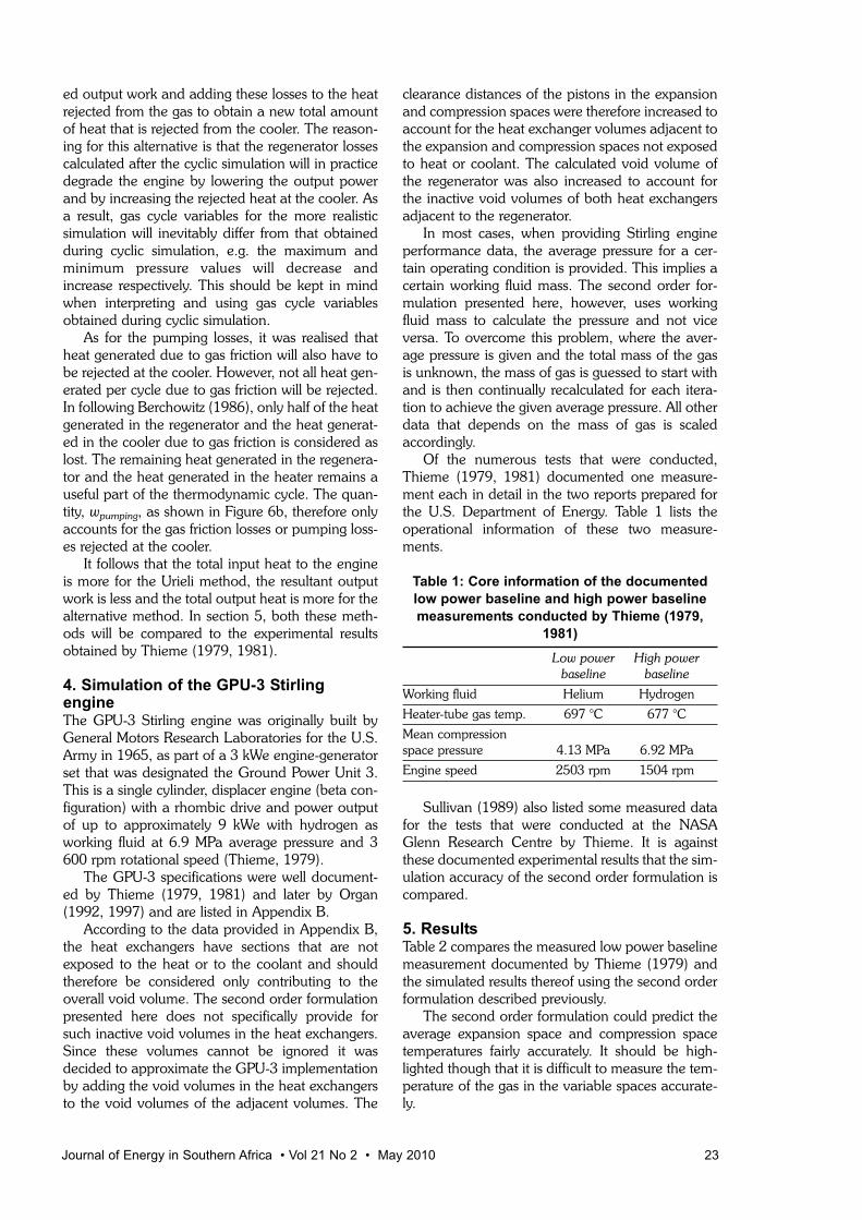
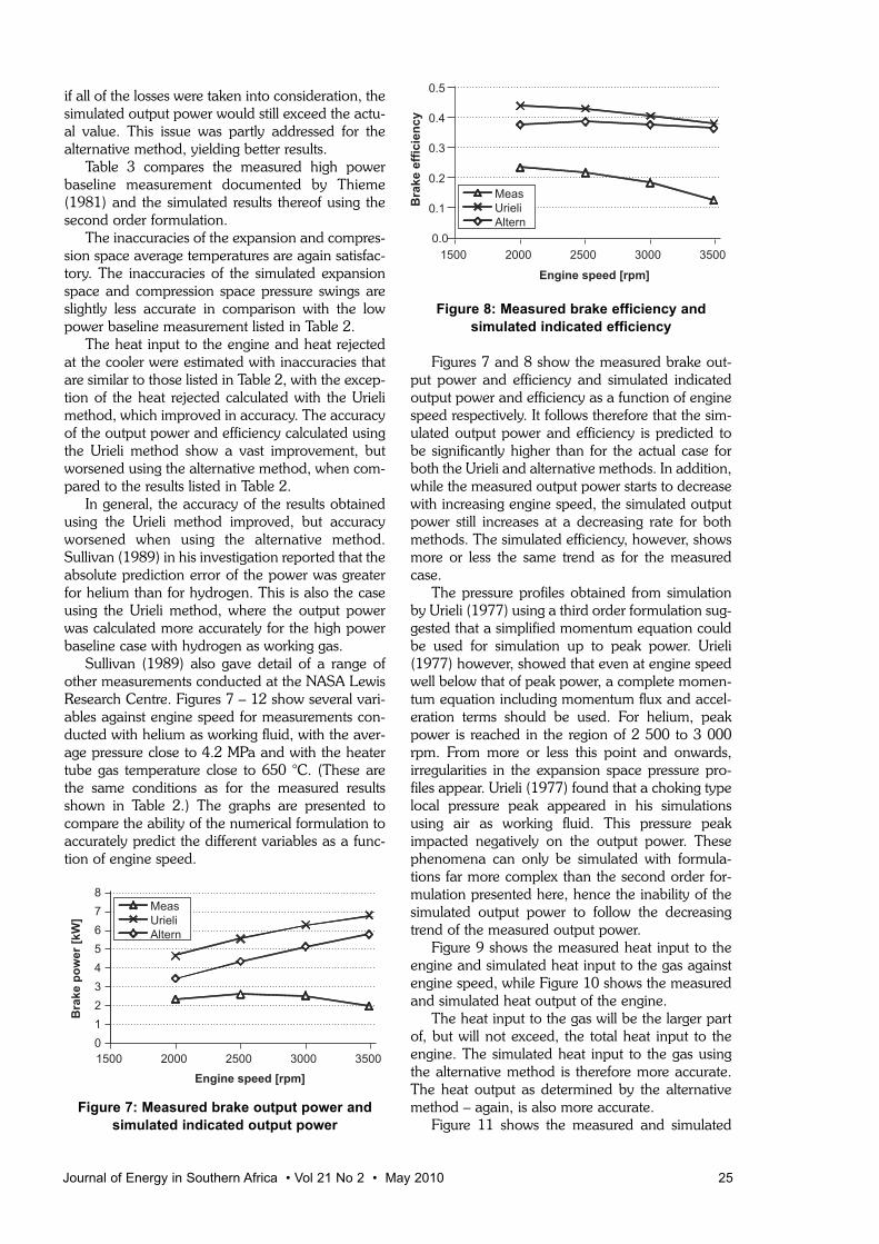
Sullivan (1989) also gave detail of a range ofother measurements conducted at the NASA LewisResearch Centre. Figures 7 – 12 show several vari-ables against engine speed for measurements con-ducted with helium as working fluid, with the aver-age pressure close to 4.2 MPa and with the heatertube gas temperature close to 650 °C. (These arethe same conditions as for the measured resultsshown in Table 2.) The graphs are presented tocompare the ability of the numerical formulation toaccurately predict the different variables as a func-tion of engine speed.

Figure 7: Measured brake output power andsimulated indicated output power

Figure 8: Measured brake efficiency andsimulated indicated efficiency

Figures 7 and 8 show the measured brake out-put power and efficiency and simulated indicatedoutput power and efficiency as a function of enginespeed respectively. It follows therefore that the sim-ulated output power and efficiency is predicted tobe significantly higher than for the actual case forboth the Urieli and alternative methods. In addition,while the measured output power starts to decreasewith increasing engine speed, the simulated outputpower still increases at a decreasing rate for bothmethods. The simulated efficiency, however, showsmore or less the same trend as for the measuredcase.

The pressure profiles obtained from simulationby Urieli (1977) using a third order formulation sug-gested that a simplified momentum equation couldbe used for simulation up to peak power. Urieli(1977) however, showed that even at engine speedwell below that of peak power, a complete momen-tum equation including momentum flux and accel-eration terms should be used. For helium, peakpower is reached in the region of 2 500 to 3 000rpm. From more or less this point and onwards,irregularities in the expansion space pressure pro-files appear. Urieli (1977) found that a choking typelocal pressure peak appeared in his simulationsusing air as working fluid. This pressure peakimpacted negatively on the output power. Thesephenomena can only be simulated with formula-tions far more complex than the second order for-mulation presented here, hence the inability of thesimulated output power to follow the decreasingtrend of the measured output power.

Figure 9 shows the measured heat input to theengine and simulated heat input to the gas againstengine speed, while Figure 10 shows the measuredand simulated heat output of the engine.

The heat input to the gas will be the larger partof, but will not exceed, the total heat input to theengine. The simulated heat input to the gas usingthe alternative method is therefore more accurate.The heat output as determined by the alternativemethod – again, is also more accurate.

Figure 11 shows the measured and simulated


expansion space pressure swing against enginespeed and Figure 12 shows the measured and sim-ulated compression space pressure swing againstengine speed.

Figure 11: Measured and simulated expansionspace pressure swing

Figure 12: Measured and simulatedcompression space pressure swing

The simulated trends for the pressure swingagainst engine speed for both the expansion spaceand compression space do not follow those of themeasured pressure swings. In the case of the expan-sion space, an increase in pressure swing is predict-ed, while the measured pressure swing shows adecrease as engine speed increases.

For the compression space, a sharply decreasingpressure swing was presented by Sullivan (1989) forincreasing engine speed for measurements withaverage pressure at close the 4.2 MPa. However,

the validity of the measured pressure swing at 3 500rpm is questioned, because no other similardecreases were observed for measurements pre-sented by Sullivan (1989) at average pressures of2.8 MPa and 5.6 MPa. The pressure swing obtainedfrom measurements at these average pressuresstayed rather constant over the same range ofengine speed. If it is indeed the case that the pres-sure swing was measured incorrectly at 3 500 rpmfor the data shown in Figure 12, then the simulatedpressure swing predicts the actual pressure swingmore accurately than for the expansion space.

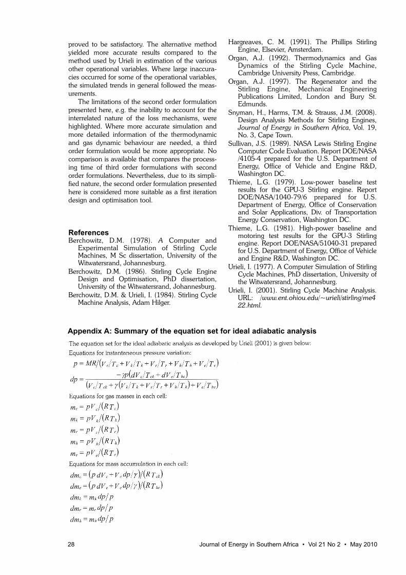
Figures 13 – 18 show several variables againstengine speed for measurements conducted withhydrogen and helium as working fluid, with theaverage pressure close to 2.8 MPa and with theheater tube gas temperature close to 700 °C.

Figures 13 and 14 show the measured brakeoutput power and efficiency and simulated indicat-ed output power and efficiency as a function ofengine speed respectively, similar to the data shownin Figures 7 and 8. The simulated output power andefficiency as predicted by the alternative methodare shown to be more accurate for both hydrogenand helium, especially at a lower engine speed. Athigher engine speed, it is shown that the simulationsbecome less accurate for reasons already discussedpreviously.

Figure 13: Measured brake output power andsimulated indicated output brake power for

hydrogen (solid line) and helium (dashed line)


Figure 9: Measured heat input to engine andsimulated heat input to gas

Figure 10: Measured and simulated heat output

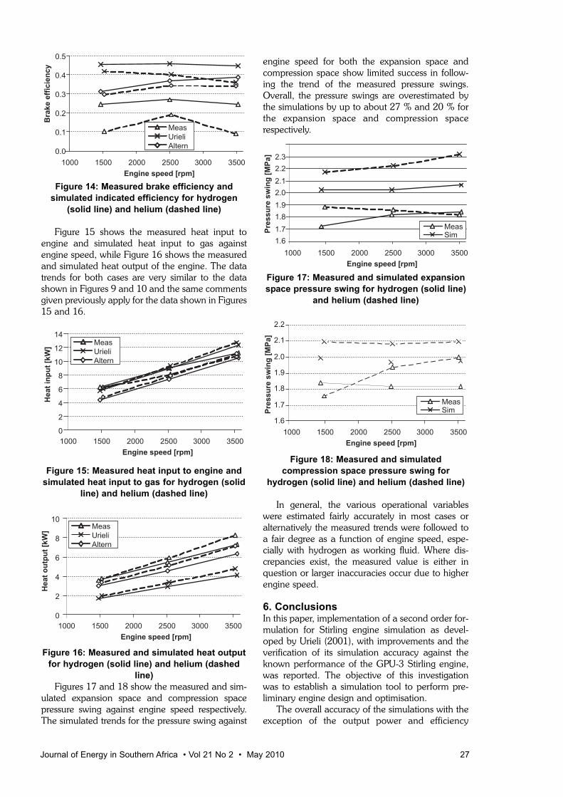
Figure 14: Measured brake efficiency andsimulated indicated efficiency for hydrogen

(solid line) and helium (dashed line)

Figure 15 shows the measured heat input toengine and simulated heat input to gas againstengine speed, while Figure 16 shows the measuredand simulated heat output of the engine. The datatrends for both cases are very similar to the datashown in Figures 9 and 10 and the same commentsgiven previously apply for the data shown in Figures15 and 16.

Figure 15: Measured heat input to engine andsimulated heat input to gas for hydrogen (solid

line) and helium (dashed line)

Figure 16: Measured and simulated heat outputfor hydrogen (solid line) and helium (dashed

line)Figures 17 and 18 show the measured and sim-

ulated expansion space and compression spacepressure swing against engine speed respectively.The simulated trends for the pressure swing against

engine speed for both the expansion space andcompression space show limited success in follow-ing the trend of the measured pressure swings.Overall, the pressure swings are overestimated bythe simulations by up to about 27 % and 20 % forthe expansion space and compression spacerespectively.

Figure 17: Measured and simulated expansionspace pressure swing for hydrogen (solid line)

and helium (dashed line)

Figure 18: Measured and simulatedcompression space pressure swing for

hydrogen (solid line) and helium (dashed line)

In general, the various operational variableswere estimated fairly accurately in most cases oralternatively the measured trends were followed toa fair degree as a function of engine speed, espe-cially with hydrogen as working fluid. Where dis-crepancies exist, the measured value is either inquestion or larger inaccuracies occur due to higherengine speed.6. ConclusionsIn this paper, implementation of a second order for-mulation for Stirling engine simulation as devel-oped by Urieli (2001), with improvements and theverification of its simulation accuracy against theknown performance of the GPU-3 Stirling engine,was reported. The objective of this investigationwas to establish a simulation tool to perform pre-liminary engine design and optimisation.

The overall accuracy of the simulations with theexception of the output power and efficiency



proved to be satisfactory. The alternative methodyielded more accurate results compared to themethod used by Urieli in estimation of the variousother operational variables. Where large inaccura-cies occurred for some of the operational variables,the simulated trends in general followed the meas-urements.

The limitations of the second order formulationpresented here, e.g. the inability to account for theinterrelated nature of the loss mechanisms, werehighlighted. Where more accurate simulation andmore detailed information of the thermodynamicand gas dynamic behaviour are needed, a thirdorder formulation would be more appropriate. Nocomparison is available that compares the process-ing time of third order formulations with secondorder formulations. Nevertheless, due to its simpli-fied nature, the second order formulation presentedhere is considered more suitable as a first iterationdesign and optimisation tool.

ReferencesBerchowitz, D.M. (1978). A Computer and

Experimental Simulation of Stirling CycleMachines, M Sc dissertation, University of theWitwatersrand, Johannesburg.

Berchowitz, D.M. (1986). Stirling Cycle EngineDesign and Optimisation, PhD dissertation,University of the Witwatersrand, Johannesburg.

Berchowitz, D.M. & Urieli, I. (1984). Stirling CycleMachine Analysis, Adam Hilger.

Hargreaves, C. M. (1991). The Phillips StirlingEngine, Elsevier, Amsterdam.

Organ, A.J. (1992). Thermodynamics and GasDynamics of the Stirling Cycle Machine,Cambridge University Press, Cambridge.

Organ, A.J. (1997). The Regenerator and theStirling Engine, Mechanical EngineeringPublications Limited, London and Bury St.Edmunds.

Snyman, H., Harms, T.M. & Strauss, J.M. (2008).Design Analysis Methods for Stirling Engines,Journal of Energy in Southern Africa, Vol. 19,No. 3, Cape Town.

Sullivan, J.S. (1989). NASA Lewis Stirling EngineComputer Code Evaluation. Report DOE/NASA/4105-4 prepared for the U.S. Department ofEnergy, Office of Vehicle and Engine R&D,Washington DC.

Thieme, L.G. (1979). Low-power baseline testresults for the GPU-3 Stirling engine. ReportDOE/NASA/1040-79/6 prepared for U.S.Department of Energy, Office of Conservationand Solar Applications, Div. of TransportationEnergy Conservation, Washington DC.

Thieme, L.G. (1981). High-power baseline andmotoring test results for the GPU-3 Stirlingengine. Report DOE/NASA/51040-31 preparedfor U.S. Department of Energy, Office of Vehicleand Engine R&D, Washington DC.

Urieli, I. (1977). A Computer Simulation of StirlingCycle Machines, PhD dissertation, University ofthe Witwatersrand, Johannesburg.

Urieli, I. (2001). Stirling Cycle Machine Analysis.URL: /www.ent.ohiou.edu/~urieli/stirling/me422.html.

Appendix A: Summary of the equation set for ideal adiabatic analysis


Appendix B: Specifications of theGeneral Motors GPU-3 Stirling engineGeneralConfiguration Single-cylinder, uniform dia-

meter bore. Rhombic drive crank mechanism

Working fluid(s) He, H2Rated maximum output 8.95 kW withHydrogen at 69 bar and 3600 rpmBore 69.9 mmStroke (piston and displacer) 31.2 mmWorking fluid circuit dimensionsHeaterMean tube length 245.3 mmLength exposed to heat source 77.7 mmTube length(cylinder side) 116.4 mmTube length (regenerator side) 128.9 mmTube inside diameter 3.02 mmTube outside diameter 4.83 mmNo. complete tubes per cylinder 40No. of tube per regenerator 5CoolerTube length 46.1 mmLength exposed to coolant 35.5 mmTube inside diameter 1.08 mmTube outside diameter 1.59 mmNo. of tubes per cylinder 312No. of tubes per regenerator 39

Compression-end connecting ductsLength 15.9 mmDuct inside diameter 5.97 mmNo. of ducts per cylinder 8Cooler end cap 279 mm3

RegeneratorsHousing inside length 22.6 mmHousing internal diameter 22.6 mmNo. regenerators per cylinder 8Mesh material Stainless steelMesh no. 7.9 wires/mmWire diameter 0.04 mmNo. of layers 308Porosity 70%Screen-to-screen rotation 5°Drive mechanismCrank eccentricity, r 13.8 mmConnecting rod length, l 46.0 mmDésaxé offset, e 20.8 mmLinear expansion space clearance 1.63 mmLinear compression space clearance 0.3 mmMinimum working space volume 232 350 mm3

Received 30 April 2009; revised 16 April 2010

21 2jesa Strauss Dobson

Documents

Transcript of 21 2jesa Strauss Dobson