2019 Ultimate tensile deformation and strength capacity of ...
111
Lakehead University Knowledge Commons,http://knowledgecommons.lakeheadu.ca Electronic Theses and Dissertations Electronic Theses and Dissertations from 2009 2019 Ultimate tensile deformation and strength capacity of shear tab connections Zhang, Chen http://knowledgecommons.lakeheadu.ca/handle/2453/4531 Downloaded from Lakehead University, KnowledgeCommons
Transcript of 2019 Ultimate tensile deformation and strength capacity of ...
Lakehead University
Knowledge Commons,http://knowledgecommons.lakeheadu.ca
Electronic Theses and Dissertations Electronic Theses and Dissertations from 2009
2019
Ultimate tensile deformation and
strength capacity of shear tab connections
Zhang, Chen
http://knowledgecommons.lakeheadu.ca/handle/2453/4531
Downloaded from Lakehead University, KnowledgeCommons
Ultimate Tensile Deformation and Strength Capacity of Shear Tab
Connections
by
Chen Zhang
A thesis
submitted to the Faculty of Graduate Studies
in partial fulfillment of requirements for the
Degree of Master of Science
in
Civil Engineering
Supervisor
Yanglin Gong, Ph.D., P.Eng.
Professor, Dept. of Civil Engineering
Co-Supervisor
Jian Deng, Ph.D., P.Eng.
Associate Professor, Dept. of Civil Engineering
Lakehead University
Thunder Bay, Ontario
June 2019
© Chen Zhang, 2019

ii
Declaration I hereby declare that I am the sole author of this thesis. This is a true copy of the thesis, including
any required final revisions, as accepted by my examiners. I understand that my thesis may be
made electronically available to the public.

iii
Abstract Single plate or shear tab is a common simple connection to connect steel beams to columns. The
connection is traditionally designed for the shear load transferred from the supported beam only,
while it has long been recognized that the shear connection can resist a certain amount of tensile
force in the longitudinal direction of the supported beam which is critical to preserve the integrity
of a structure. Canadian standard CSA/S16-14 explicitly states that connections shall be designed
to provide resistance to progressive collapse as a consequence of a local failure. However, few
specific design requirements are provided in the standard. Hence, the main objective of this
research is to quantify the deformation and strength capacities of shear-tab connections when
subjected to a pure tension or a combined tension and shear load in the context of progressive
collapse resistance.
First, a set of full-scale shear tab connection specimens were tested under a pure tension load.
The results from the experiments are then used to verify and calibrate a finite element model of
the connections. Thirdly, the finite element model is used to conduct a parametric study to
determine the impact of tab thickness, tab edge distance, bolt diameter and the combined effect of
tension and shear load. Finally, a formulation describing the relationship between the tensile force
and the axial deformation for the shear tab connections is developed.

iv
Acknowledgements This research would not be successful without the help of many people that I owe a debt of
gratitude. I would like to express my gratitude to all those who helped me during the course of this
thesis.
First, my deepest gratitude goes to Professor Yanglin Gong, my supervisor, for his constant
encouragement and guidance. Dr. Gong has walked me through all the stages of this research.
Without his patient instruction, insight criticism and expert guidance, the completion of this thesis
would not have been possible. Also, I would like to thank my co-supervisor, Professor Jian Deng,
whose support, knowledge and experience helped me tremendously during the research.
I would like to thank Professor Sam Salem for serving as a thesis committee member. My
gratitude is also due to Professor Hao Bai for serving as the external thesis examiner.
I would like to thank students Blake Peters, Daniel Leung, Thomas Wipf and Asparukh
Akanayev, for assistance in executing the laboratory work. Thank you for spending your reading
week by my side at Lakehead University Structure Laboratory.
I would like to extend my appreciation to my parents who gave me their love and support
throughout my studies. Last, but not least, a special thanks to my fiancée, with her support, patience
and understanding throughout this research, I have completed this thesis.
v
Contents Abstract ………………………………………………………………………………..…………iii
Acknowledgements …………………………………………………………...………………….iv
Contents …………………………………………………………………………………...............v
List of Tables ………………….………………………………………………………………...viii
List of Figures ……………...……………………………………………………………………..ix
Chapter 1 Introduction ………………………………………………………….……….1
1.1 Research consideration and objectives …………………………………………………….1
1.2 Lab tests of shear tab connection ……………………………..……………………………3
1.3 Finite element modeling of shear tab connections ………………………………...……….9
1.4 Design guideline for shear tab connections ………………………………………………12
1.5 Thesis Outline ……………………………………………………………………………..13
Chapter 2 Experimental test ……………………………………………………..……..14
2.1 Test setup and design ……………………………………………………………………...14
2.2 Test procedure ……………………………………………………………………………..22
2.3 Test results …………………………………………………………………………………23
2A Appendix Coupon test ……………………………………………………………………..33
Chapter 3 Finite element modeling ……………………………………………….……38
3.1 Modeling process ………………………………………………………………………….38
3.1.1 Generating the geometry …………………………………………………………….38
3.1.2 Inputting material property ………………………………………………………….40
3.1.3 Assembly ……………………………………………………………………………50
3.1.4 Setting analysis step …………………………………………………………………51
3.1.5 Applying interaction ………………………………………………………………...51
3.1.6 Applying load ……………………………………………………………………….52
3.1.7 Mesh design …………………………………………………………………………53
3.1.8 Job …………………………………………………………………………………..53
3.1.9 Visualization ………………………………………………………………………...54
3.2 Simulation results …………………………………………………………………………54
T95-45-1 …………………………………………………………………………………..54
T95-57-1 …………………………………………………………………………………..55
vi
T127-45-1 ……………………………………………………………………………........56
T95-45-2 …………………………………………………………………………………..57
T127-45-2 ……………………………………………………………………………........58
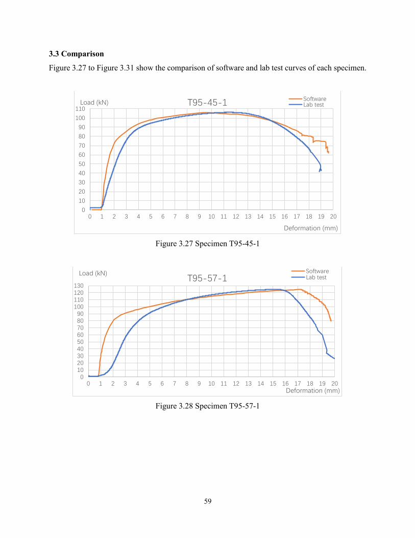
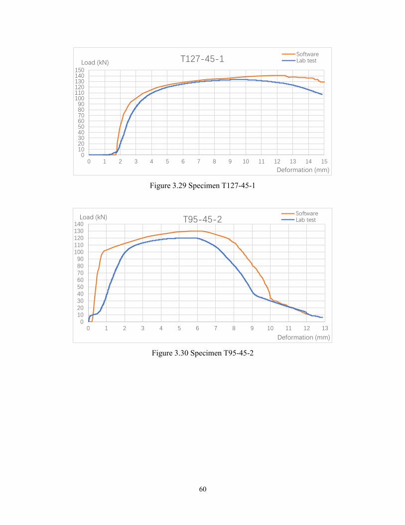
3.3 Comparison ……………………………………………………………………………….59
T95-45-1 …………………………………………………………………………………..59
T95-57-1 …………………………………………………………………………………..59
T127-45-1 ……………………………………………………………………………........60
T95-45-2 …………………………………………………………………………………..60
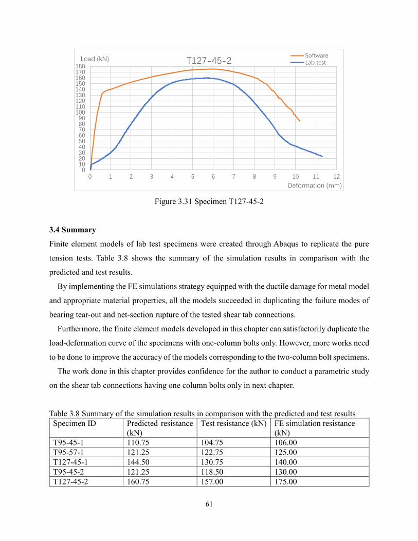
T127-45-2 ……………………………………………………………………………........61
3.4 Summary ………………………………………………………………………………….61
Chapter 4 Parametric study ……………………………………………………………62
4.1 Parameters ………………………………………………………………………………...62
4.2 Simulation results of 19mm bolt diameter ………………………………………………...62
T95-38-1 ……………………………………………………………………………..........63
T95-48-1 ……………………………………………………………………………..........64
T64-38-1 ……………………………………………………………………………..........65
T64-48-1 ……………………………………………………………………………..........66
T127-38-1 …………………………………………………………………………………67
T127-48-1 …………………………………………………………………………………68
4.3 Simulation results of 22.2mm bolt diameter ………………………………………………68
T64-45-1 …………………………………………………………………………………..69
T64-57-1 …………………………………………………………………………………..70
T127-57-1 …………………………………………………………………………………71
4.4 Simulation results of 25.4mm bolt diameter ………………………………………………71
T95-51-1 …………………………………………………………………………………..72
T95-64-1 …………………………………………………………………………………..73
T64-51-1 …………………………………………………………………………………..74
T64-64-1 …………………………………………………………………………………..75
T127-51-1 …………………………………………………………………………………76
T127-64-1 …………………………………………………………………………………77
4.5 Simulation results of combined tension and shear …………………………………..……..77
vii
4.6 Observations ………………………………………………………………………………79
Chapter 5 Analysis of the load versus deformation curve …………………………….80
5.1 The method of a tri-linear curve …………………………………………………………...80
5.2 Determination of Ty and Δy ………………………………………………………………...81
5.3 Determination of Tu and Δu ………………………………………………………………..85
5.4 Determination of Tr and Δr ………………………………………………………………...91
Chapter 6 Conclusions and future works …………………………………………..….95
6.1 Summary and conclusions ………………………………………………………………...95
6.2 Future works ……………………………….……………………………………………...96
References ……………………………………………………………………………………....97
viii
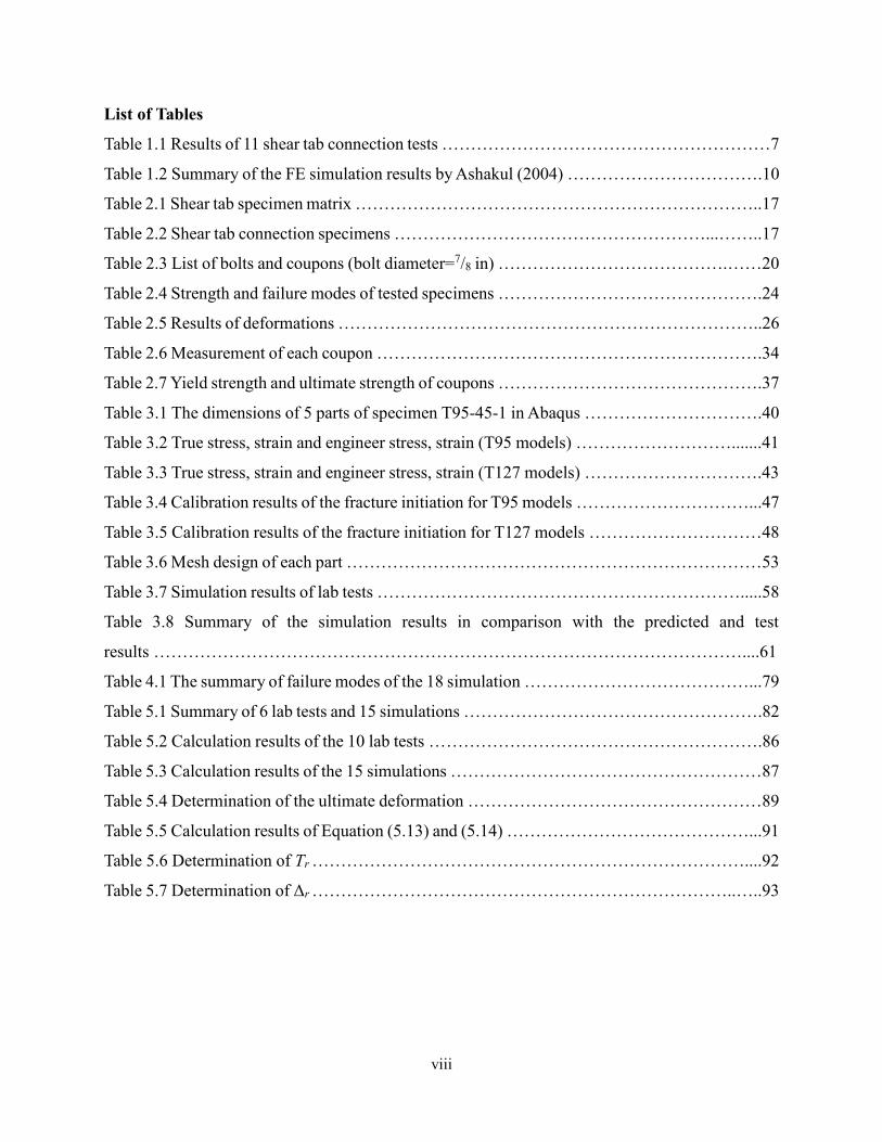
List of Tables
Table 1.1 Results of 11 shear tab connection tests …………………………………………………7
Table 1.2 Summary of the FE simulation results by Ashakul (2004) …………………………….10
Table 2.1 Shear tab specimen matrix ……………………………………………………………..17
Table 2.2 Shear tab connection specimens ………………………………………………...……..17
Table 2.3 List of bolts and coupons (bolt diameter=7/8 in) ………………………………….……20
Table 2.4 Strength and failure modes of tested specimens ……………………………………….24
Table 2.5 Results of deformations ………………………………………………………………..26
Table 2.6 Measurement of each coupon ………………………………………………………….34
Table 2.7 Yield strength and ultimate strength of coupons ……………………………………….37
Table 3.1 The dimensions of 5 parts of specimen T95-45-1 in Abaqus ………………………….40
Table 3.2 True stress, strain and engineer stress, strain (T95 models) ……………………….......41
Table 3.3 True stress, strain and engineer stress, strain (T127 models) ………………………….43
Table 3.4 Calibration results of the fracture initiation for T95 models …………………………...47
Table 3.5 Calibration results of the fracture initiation for T127 models …………………………48
Table 3.6 Mesh design of each part ………………………………………………………………53
Table 3.7 Simulation results of lab tests ……………………………………………………….....58
Table 3.8 Summary of the simulation results in comparison with the predicted and test
results …………………………………………………………………………………………....61
Table 4.1 The summary of failure modes of the 18 simulation …………………………………...79
Table 5.1 Summary of 6 lab tests and 15 simulations …………………………………………….82
Table 5.2 Calculation results of the 10 lab tests ………………………………………………….86
Table 5.3 Calculation results of the 15 simulations ………………………………………………87
Table 5.4 Determination of the ultimate deformation ……………………………………………89
Table 5.5 Calculation results of Equation (5.13) and (5.14) ……………………………………...91
Table 5.6 Determination of Tr …………………………………………………………………....92
Table 5.7 Determination of Δr ………………………………………………………………..…..93
ix
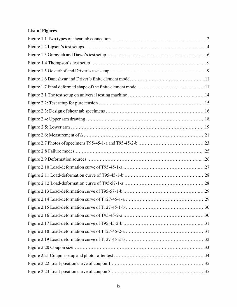
List of Figures
Figure 1.1 Two types of shear tab connection ……………………………………………….…….2
Figure 1.2 Lipson’s test setups …………………………………………………………………….4
Figure 1.3 Guravich and Dawe’s test setup ………………………………………………….…….6
Figure 1.4 Thompson’s test setup ……………………………………………………………...…8
Figure 1.5 Oosterhof and Driver’ s test setup …………………………………………………..….9
Figure 1.6 Daneshvar and Driver’s finite element model ………………………………………...11
Figure 1.7 Final deformed shape of the finite element model …………………………….………11
Figure 2.1 The test setup on universal testing machine …………………………………….…….14
Figure 2.2: Test setup for pure tension …………………………………………………………...15
Figure 2.3: Design of shear tab specimens ……………………………………………………….16
Figure 2.4: Upper arm drawing ……………………………………………….………….………18
Figure 2.5: Lower arm ………………………………………………………………….………..19
Figure 2.6: Measurement of Δ ……………………………………………………………………21
Figure 2.7 Photos of specimens T95-45-1-a and T95-45-2-b …………………………………….23
Figure 2.8 Failure modes ………………………………………………………………………...25
Figure 2.9 Deformation sources …………………………………………………………….…....26
Figure 2.10 Load-deformation curve of T95-45-1-a ………………………………………….….27
Figure 2.11 Load-deformation curve of T95-45-1-b ………………………………………….…28
Figure 2.12 Load-deformation curve of T95-57-1-a …………………………………………….28
Figure 2.13 Load-deformation curve of T95-57-1-b ………………………………………….….29
Figure 2.14 Load-deformation curve of T127-45-1-a ……………………………………………29
Figure 2.15 Load-deformation curve of T127-45-1-b ……………………………………………30
Figure 2.16 Load-deformation curve of T95-45-2-a ……………………………………….…….30
Figure 2.17 Load-deformation curve of T95-45-2-b ………………………………………….….31
Figure 2.18 Load-deformation curve of T127-45-2-a ……………………………………………31
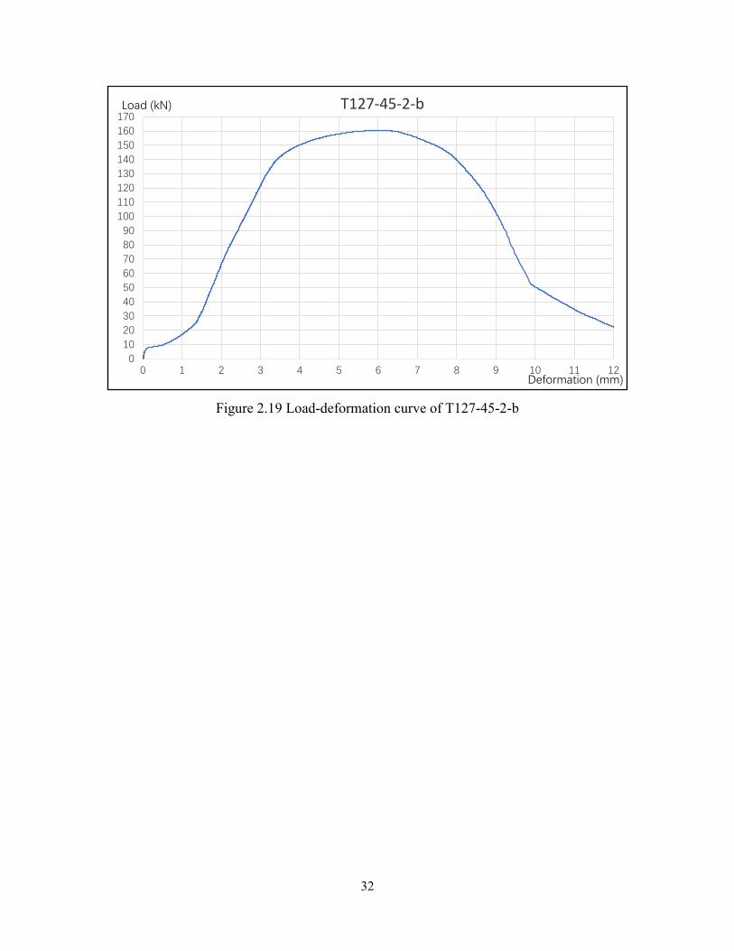
Figure 2.19 Load-deformation curve of T127-45-2-b ……………………………………………32
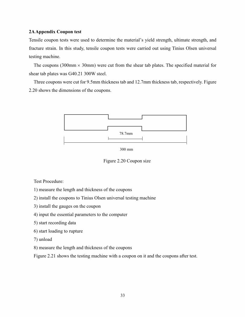
Figure 2.20 Coupon size………………………………………………………………………….33
Figure 2.21 Coupon setup and photos after test …………………………………………….…….34
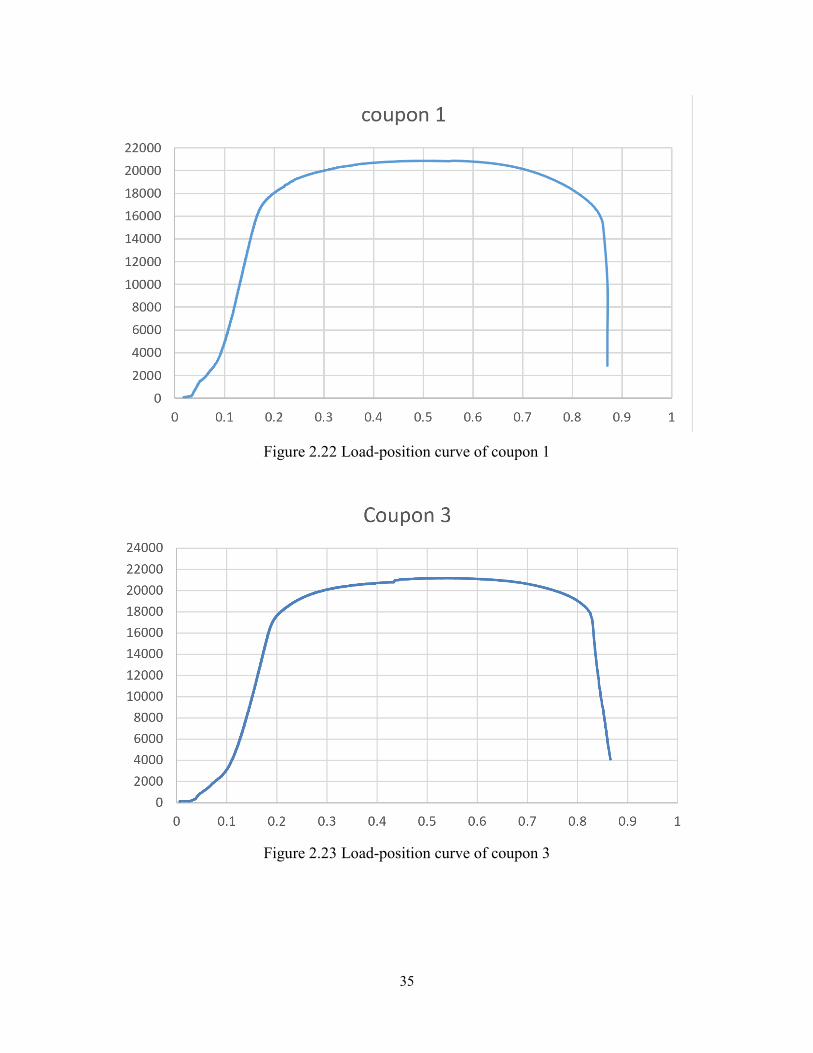
Figure 2.22 Load-position curve of coupon 1 ……………………………………………………35
Figure 2.23 Load-position curve of coupon 3 ……………………………………………………35
x
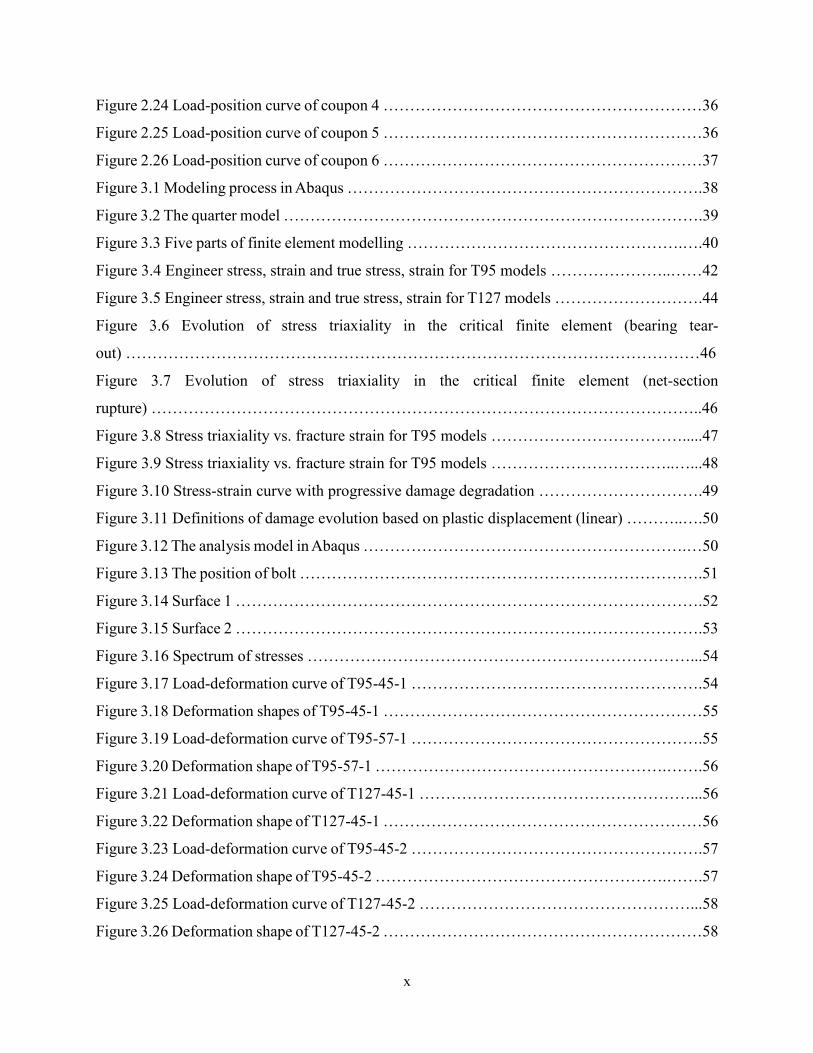
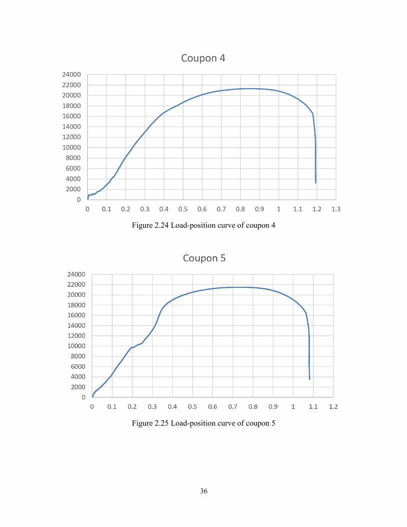
Figure 2.24 Load-position curve of coupon 4 ……………………………………………………36
Figure 2.25 Load-position curve of coupon 5 ……………………………………………………36
Figure 2.26 Load-position curve of coupon 6 ……………………………………………………37
Figure 3.1 Modeling process in Abaqus ………………………………………………………….38
Figure 3.2 The quarter model …………………………………………………………………….39
Figure 3.3 Five parts of finite element modelling …………………………………………….….40
Figure 3.4 Engineer stress, strain and true stress, strain for T95 models …………………..……42
Figure 3.5 Engineer stress, strain and true stress, strain for T127 models ……………………….44
Figure 3.6 Evolution of stress triaxiality in the critical finite element (bearing tear-
out) ………………………………………………………………………………………………46
Figure 3.7 Evolution of stress triaxiality in the critical finite element (net-section
rupture) …………………………………………………………………………………………..46
Figure 3.8 Stress triaxiality vs. fracture strain for T95 models ……………………………….....47
Figure 3.9 Stress triaxiality vs. fracture strain for T95 models ……………………………..…...48
Figure 3.10 Stress-strain curve with progressive damage degradation ………………………….49
Figure 3.11 Definitions of damage evolution based on plastic displacement (linear) ………..….50
Figure 3.12 The analysis model in Abaqus …………………………………………………….…50
Figure 3.13 The position of bolt ………………………………………………………………….51
Figure 3.14 Surface 1 …………………………………………………………………………….52
Figure 3.15 Surface 2 …………………………………………………………………………….53
Figure 3.16 Spectrum of stresses ………………………………………………………………...54
Figure 3.17 Load-deformation curve of T95-45-1 ……………………………………………….54
Figure 3.18 Deformation shapes of T95-45-1 ……………………………………………………55
Figure 3.19 Load-deformation curve of T95-57-1 ……………………………………………….55
Figure 3.20 Deformation shape of T95-57-1 ……………………………………………….…….56
Figure 3.21 Load-deformation curve of T127-45-1 ……………………………………………...56
Figure 3.22 Deformation shape of T127-45-1 ……………………………………………………56
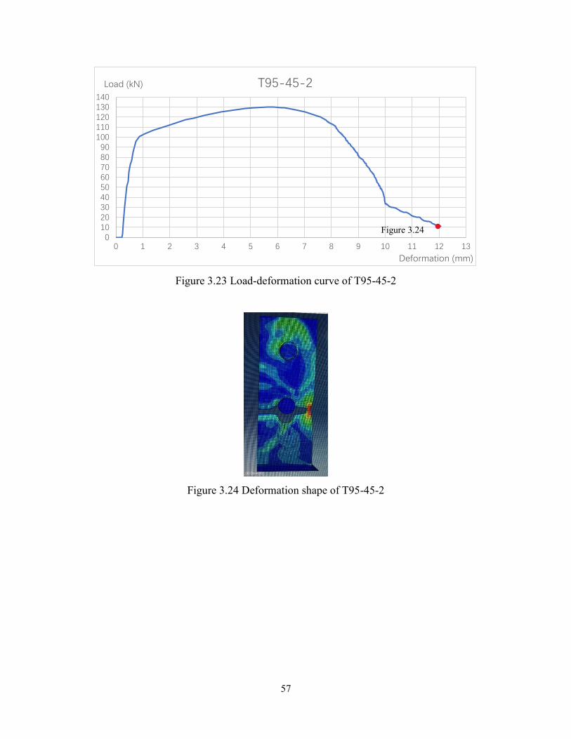
Figure 3.23 Load-deformation curve of T95-45-2 ……………………………………………….57
Figure 3.24 Deformation shape of T95-45-2 ……………………………………………….…….57
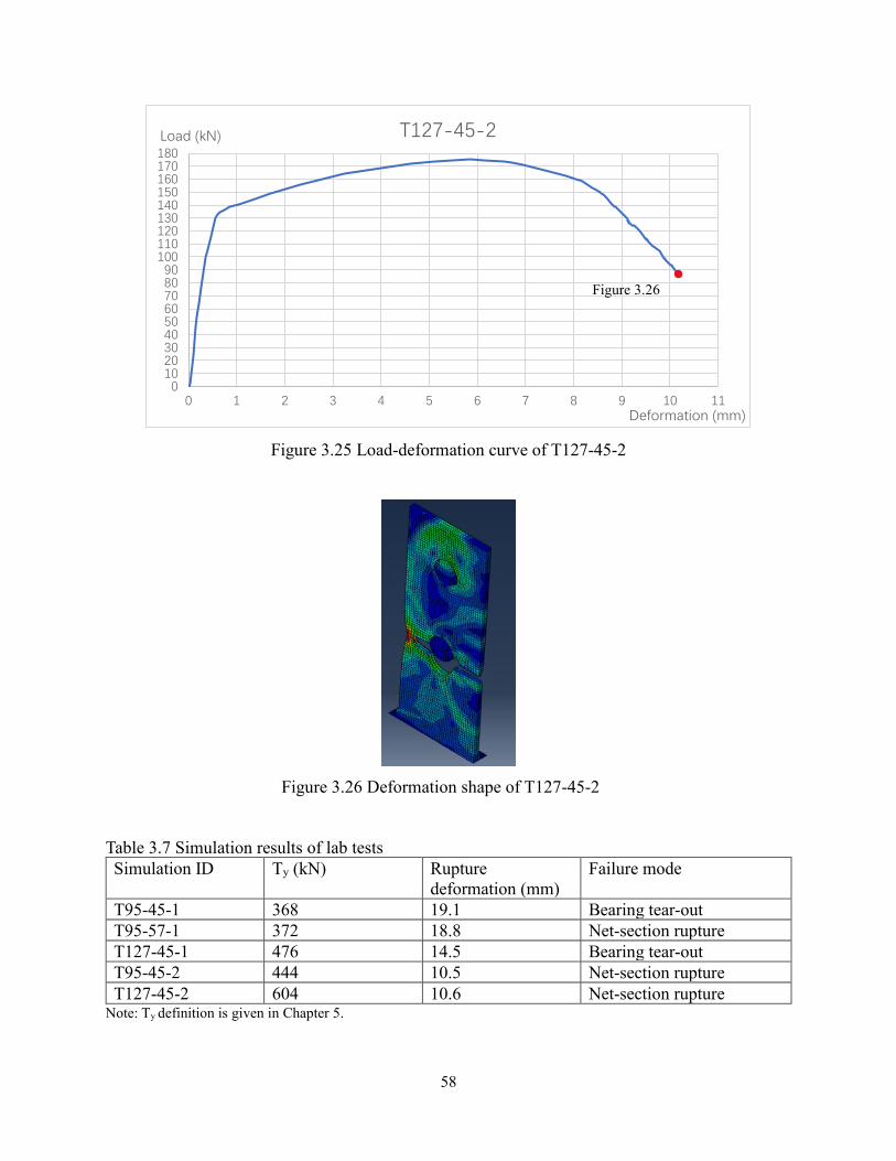
Figure 3.25 Load-deformation curve of T127-45-2 ……………………………………………...58
Figure 3.26 Deformation shape of T127-45-2 ……………………………………………………58
xi
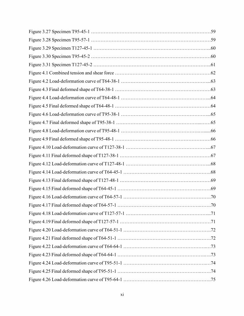
Figure 3.27 Specimen T95-45-1 …………………………………………………………………59
Figure 3.28 Specimen T95-57-1 …………………………………………………………………59
Figure 3.29 Specimen T127-45-1 ………………………………………………………………..60
Figure 3.30 Specimen T95-45-2 …………………………………………………………………60
Figure 3.31 Specimen T127-45-2 ………………………………………………………………..61
Figure 4.1 Combined tension and shear force ……………………………………………………62
Figure 4.2 Load-deformation curve of T64-38-1 ………………………………………………...63
Figure 4.3 Final deformed shape of T64-38-1 ……………………………………………………63
Figure 4.4 Load-deformation curve of T64-48-1 ………………………………………………...64
Figure 4.5 Final deformed shape of T64-48-1 ……………………………………………………64
Figure 4.6 Load-deformation curve of T95-38-1 ………………………………………………...65
Figure 4.7 Final deformed shape of T95-38-1 ……………………………………………...……65
Figure 4.8 Load-deformation curve of T95-48-1 ………………………………………….…......66
Figure 4.9 Final deformed shape of T95-48-1 ……………………………………………………66
Figure 4.10 Load-deformation curve of T127-38-1 ……………………………………………...67
Figure 4.11 Final deformed shape of T127-38-1 …………………………………………………67
Figure 4.12 Load-deformation curve of T127-48-1 ……………………………………………...68
Figure 4.14 Load-deformation curve of T64-45-1 ……………………………………………….68
Figure 4.13 Final deformed shape of T127-48-1 …………………………………………………69
Figure 4.15 Final deformed shape of T64-45-1 …………………………………………….…….69
Figure 4.16 Load-deformation curve of T64-57-1 ……………………………………………….70
Figure 4.17 Final deformed shape of T64-57-1 …………………………………………….…….70
Figure 4.18 Load-deformation curve of T127-57-1 ……………………………………………...71
Figure 4.19 Final deformed shape of T127-57-1 …………………………………………………71
Figure 4.20 Load-deformation curve of T64-51-1 ……………………………………………….72
Figure 4.21 Final deformed shape of T64-51-1 …………………………………………….…….72
Figure 4.22 Load-deformation curve of T64-64-1 …………………………………………….…73
Figure 4.23 Final deformed shape of T64-64-1 ……………………………………………….….73
Figure 4.24 Load-deformation curve of T95-51-1 …………………………………………….…74
Figure 4.25 Final deformed shape of T95-51-1 …………………………………………….…….74
Figure 4.26 Load-deformation curve of T95-64-1 ……………………………………………….75
xii
Figure 4.27 Final deformed shape of T95-64-1 ……………………………………………….….75
Figure 4.28 Load-deformation curve of T127-51-1 ……………………………………………...76
Figure 4.29 Final deformed shape of T127-51-1 …………………………………………………76
Figure 4.30 Load-deformation curve of T127-64-1 ……………………………………………...77
Figure 4.31 Final deformed shape of T127-64-1 …………………………………………………77
Figure 4.32 Load vs. deformation of T95-45-1 under combined tension and shear ………….…78
Figure 4.33 Failure modes of T95-45-1 under combined tension and shear ………………….....78
Figure 5.1 Tri-linear curve of T95-45-1 ………………………………………………………….80
Figure 5.2 Load versus deformation of a nonlinear spring ………………………………………81
Figure 5.3 Determination of Ty …………………………………………………………………..83
Figure 5.4 Determination of Ky …………………………………………………………………..84
Figure 5.5 Block shear failure ……………………………………………………………………85
Figure 5.6 Determination of ∆u …………………………………………………………………..90
Figure 5.7 Determination of Tr …………………………………………………………………...92
Figure 5.8 Determination of Δr …………………………………………………………………..94
Figure 6.1 Failure modes when V 0.45T ………………………………………………………..96
1
Chapter 1 Introduction
This chapter provides a general background about shear tab connections and the reasons of this
study. Research objectives and literature review are listed, and the outline of the thesis is presented.
1.1 Research considerations and objectives
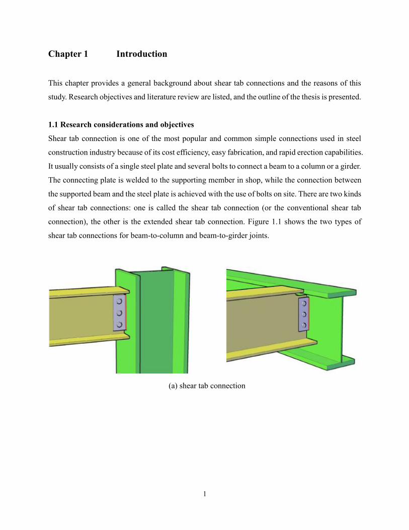
Shear tab connection is one of the most popular and common simple connections used in steel
construction industry because of its cost efficiency, easy fabrication, and rapid erection capabilities.
It usually consists of a single steel plate and several bolts to connect a beam to a column or a girder.
The connecting plate is welded to the supporting member in shop, while the connection between
the supported beam and the steel plate is achieved with the use of bolts on site. There are two kinds
of shear tab connections: one is called the shear tab connection (or the conventional shear tab
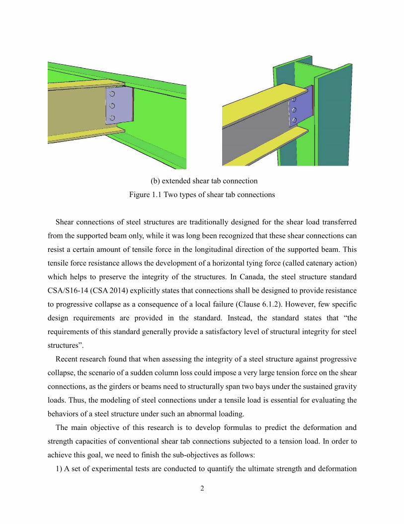
connection), the other is the extended shear tab connection. Figure 1.1 shows the two types of
shear tab connections for beam-to-column and beam-to-girder joints.
(a) shear tab connection
2
(b) extended shear tab connection
Figure 1.1 Two types of shear tab connections
Shear connections of steel structures are traditionally designed for the shear load transferred
from the supported beam only, while it was long been recognized that these shear connections can
resist a certain amount of tensile force in the longitudinal direction of the supported beam. This
tensile force resistance allows the development of a horizontal tying force (called catenary action)
which helps to preserve the integrity of the structures. In Canada, the steel structure standard
CSA/S16-14 (CSA 2014) explicitly states that connections shall be designed to provide resistance
to progressive collapse as a consequence of a local failure (Clause 6.1.2). However, few specific
design requirements are provided in the standard. Instead, the standard states that “the
requirements of this standard generally provide a satisfactory level of structural integrity for steel
structures”.
Recent research found that when assessing the integrity of a steel structure against progressive
collapse, the scenario of a sudden column loss could impose a very large tension force on the shear
connections, as the girders or beams need to structurally span two bays under the sustained gravity
loads. Thus, the modeling of steel connections under a tensile load is essential for evaluating the
behaviors of a steel structure under such an abnormal loading.
The main objective of this research is to develop formulas to predict the deformation and
strength capacities of conventional shear tab connections subjected to a tension load. In order to
achieve this goal, we need to finish the sub-objectives as follows:
1) A set of experimental tests are conducted to quantify the ultimate strength and deformation
3
capacities of shear tab connections subjected to a pure tension load.
2) The results from the experiments will be used to verify a finite element model of the
connections.
3) The finite element model will be used to conduct a parametric study.
4) Finally, a formulation describing the relationship between the tensile force and the tensile
deformation of the shear tab connections will be developed.
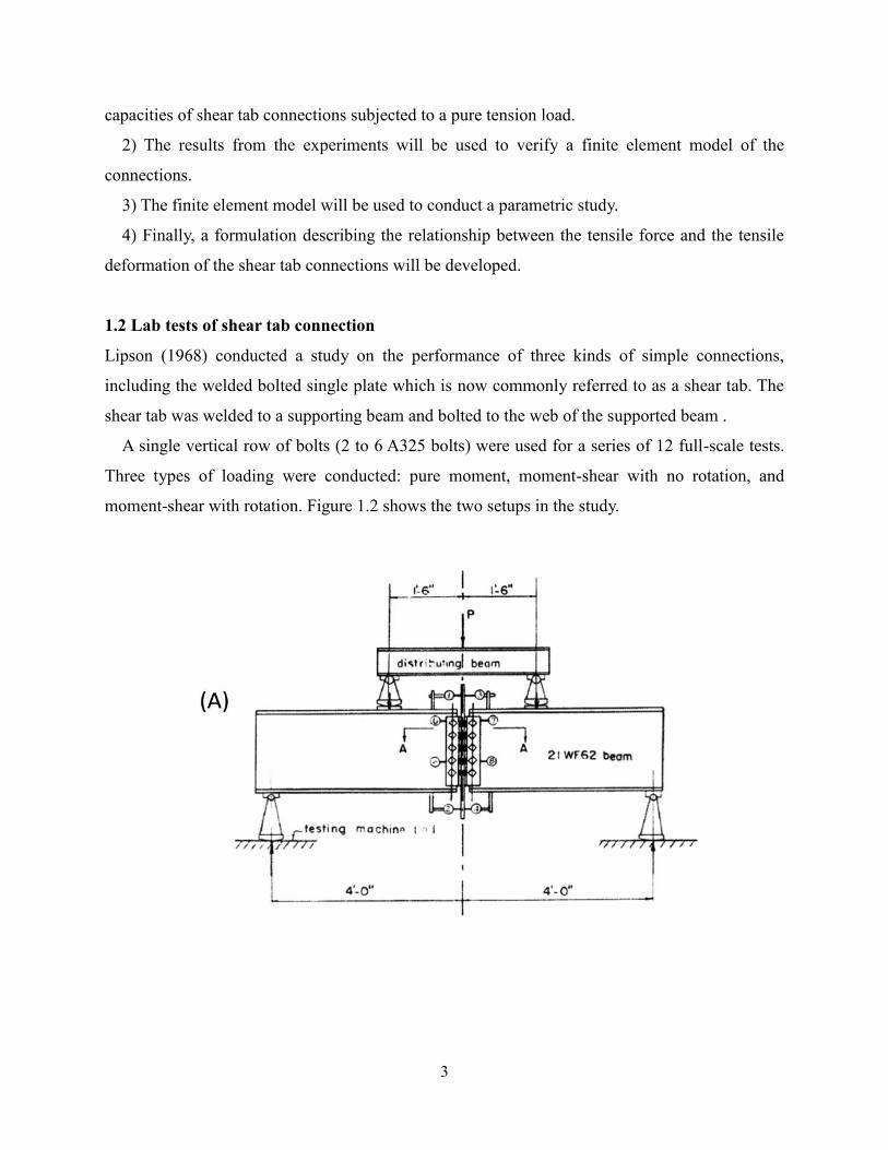
1.2 Lab tests of shear tab connection Lipson (1968) conducted a study on the performance of three kinds of simple connections,
including the welded bolted single plate which is now commonly referred to as a shear tab. The
shear tab was welded to a supporting beam and bolted to the web of the supported beam .
A single vertical row of bolts (2 to 6 A325 bolts) were used for a series of 12 full-scale tests.
Three types of loading were conducted: pure moment, moment-shear with no rotation, and
moment-shear with rotation. Figure 1.2 shows the two setups in the study.
4
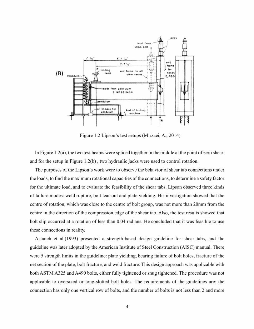
Figure 1.2 Lipson’s test setups (Mirzaei, A., 2014)
In Figure 1.2(a), the two test beams were spliced together in the middle at the point of zero shear,
and for the setup in Figure 1.2(b) , two hydraulic jacks were used to control rotation.
The purposes of the Lipson’s work were to observe the behavior of shear tab connections under
the loads, to find the maximum rotational capacities of the connections, to determine a safety factor
for the ultimate load, and to evaluate the feasibility of the shear tabs. Lipson observed three kinds
of failure modes: weld rupture, bolt tear-out and plate yielding. His investigation showed that the
centre of rotation, which was close to the centre of bolt group, was not more than 20mm from the
centre in the direction of the compression edge of the shear tab. Also, the test results showed that
bolt slip occurred at a rotation of less than 0.04 radians. He concluded that it was feasible to use
these connections in reality.
Astaneh et al.(1993) presented a strength-based design guideline for shear tabs, and the
guideline was later adopted by the American Institute of Steel Construction (AISC) manual. There
were 5 strength limits in the guideline: plate yielding, bearing failure of bolt holes, fracture of the
net section of the plate, bolt fracture, and weld fracture. This design approach was applicable with
both ASTM A325 and A490 bolts, either fully tightened or snug tightened. The procedure was not
applicable to oversized or long-slotted bolt holes. The requirements of the guidelines are: the
connection has only one vertical row of bolts, and the number of bolts is not less than 2 and more
5
than 7; bolt spacing is equal to 76 mm; edge distances are equal to or greater than 1.5d, where d is
the diameter of the bolts, and the vertical edge distance for the lowest bolt is preferred not to be
less than 38 mm; thickness of the single plate should be less than or equal to d/2 + 1/16 in; the ratio
of c/d of the plate should be greater than or equal to 2 to prevent local buckling of the plate, where
c is edge distance; the distance between the bolt line and the weld line was limited to 64-76 mm;
the size of the connecting fillet weld was required to be greater than 0.75t, where t is the thickness
of the shear tab.
A series of test specimens was designed with this approach, and the test results showed that the
ductile and tolerated rotations was from 0.026 to 0.061 radians at the point of the maximum shear.
The number of bolts influenced the rotational ductility; i.e., the higher the number of bolts, the
lower the rotational ductility that could be achieved. At last, the experimental studies indicated that
considerable shear and bearing yielding occurred in the plate before the failure. The yielding would
decrease the rotational stiffness which would cause the reduction of the end moments of the
supported beam.
Guravich and Dawe (2006) tested 108 full-scale shear tab connections. Their main goal was to
investigate the performance of shear tab connections under the effect of combined shear, moment
and tension force.
They used a single row of 3 bolts (3/4 inch ASTM A325) to connect the shear tab (7.9mm
thickness), which was commonly used at that time. Figure 1.3 shows the test setup.
6
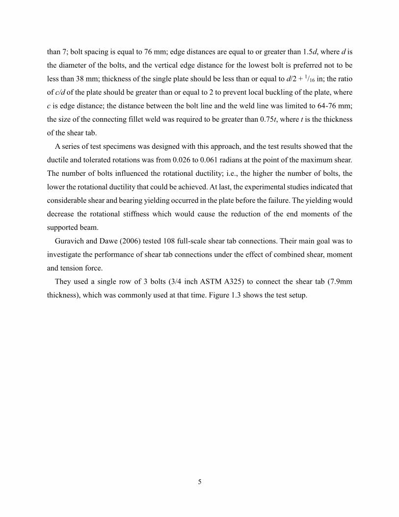
Figure 1.3 Guravich and Dawe’s test setup (Mirzaei, A., 2014)
Two vertical W310 × 97 reaction columns were fixed to the rigid ground while two horizontal
W610 × 155 reaction beams were framed to the two columns. The upper beam was the support for
cylinder D, and the lower beam acted as a rigid support for the specimens. Shear tabs were welded
to a steel plate which was bolted onto the lower beam. Five hydraulic cylinders were used: A
applied the main shear force to the connection; B and C controlled the rotation of the connection;
D applied the tension force; E controlled the position of cylinder D to keep the force perpendicular
to the beams . The test procedures were as follows:
1) rotated the test beam to 0.03 radians and applied the desired value of shear force (either half
7
or total of the factored bolt shear capacity)
2) applied the axial tension to the test beam (the rotation and shear force remain unchanged
during the testing)
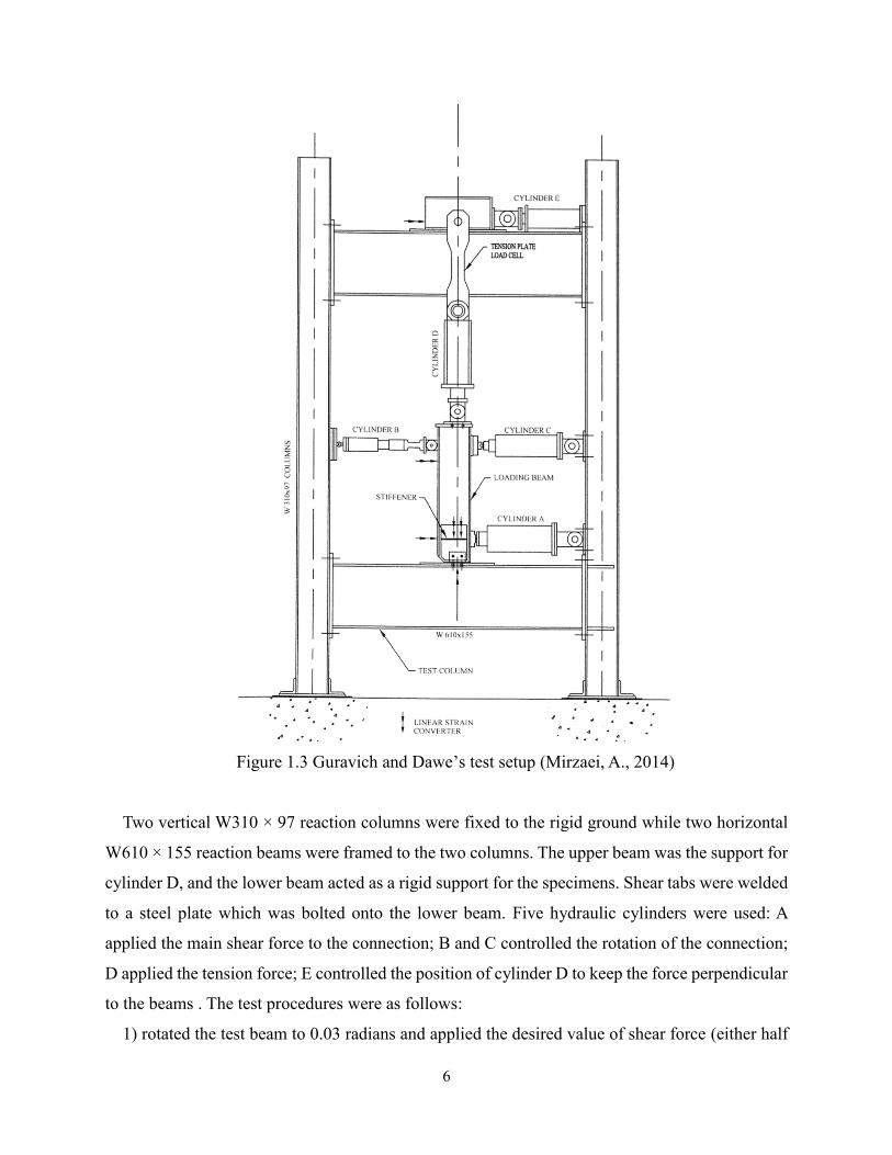
Table 1.1 shows the results of 11 shear tab connection tests.
Table 1.1 Results of 11 shear tab connection tests.
Notes: Vtest: Applied shear load; Tult: ultimate tension load; Vres: Resultant shear force; Bp: Bearing resistance of shear tabs.
From Table 1.1, T308-1 and T308-2 failed with plate buckling failure under pure shear load, and
all other tests failed with steel plate shear fracture. Also, from the average ratio of Vres/Bp of 0.94,
they concluded that Bp was a key factor to determine the ultimate resistance capacity of shear tab
connection under combined shear and tension load.
Thompson (2009) investigated 9 full-scale tests of shear tab connections under a scenario of
column removal. His main goal was to determine the stability of the shear tab connections and
their ability for the catenary action. Figure 1.4 shows the test setup.
8
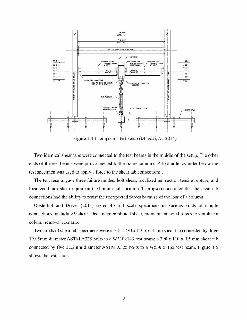
Figure 1.4 Thompson’s test setup (Mirzaei, A., 2014)
Two identical shear tabs were connected to the test beams in the middle of the setup. The other
ends of the test beams were pin-connected to the frame columns. A hydraulic cylinder below the
test specimen was used to apply a force to the shear tab connections .
The test results gave three failure modes: bolt shear, localized net section tensile rupture, and
localized block shear rupture at the bottom bolt location. Thompson concluded that the shear tab
connections had the ability to resist the unexpected forces because of the loss of a column.
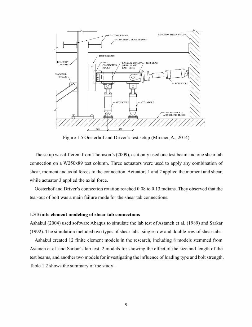
Oosterhof and Driver (2011) tested 45 full scale specimens of various kinds of simple
connections, including 9 shear tabs, under combined shear, moment and axial forces to simulate a
column removal scenario.
Two kinds of shear tab specimens were used: a 230 x 110 x 6.4 mm shear tab connected by three
19.05mm diameter ASTM A325 bolts to a W310x143 test beam; a 390 x 110 x 9.5 mm shear tab
connected by five 22.2mm diameter ASTM A325 bolts to a W530 x 165 test beam. Figure 1.5
shows the test setup.
9
Figure 1.5 Oosterhof and Driver’s test setup (Mirzaei, A., 2014)
The setup was different from Thomson’s (2009), as it only used one test beam and one shear tab
connection on a W250x89 test column. Three actuators were used to apply any combination of
shear, moment and axial forces to the connection. Actuators 1 and 2 applied the moment and shear,
while actuator 3 applied the axial force.
Oosterhof and Driver’s connection rotation reached 0.08 to 0.13 radians. They observed that the
tear-out of bolt was a main failure mode for the shear tab connections.
1.3 Finite element modeling of shear tab connections
Ashakul (2004) used software Abaqus to simulate the lab test of Astaneh et al. (1989) and Sarkar
(1992). The simulation included two types of shear tabs: single-row and double-row of shear tabs.
Ashakul created 12 finite element models in the research, including 8 models stemmed from
Astaneh et al. and Sarkar’s lab test, 2 models for showing the effect of the size and length of the
test beams, and another two models for investigating the influence of loading type and bolt strength.
Table 1.2 shows the summary of the study .
10
Table 1.2 Summary of the FE simulation results by Ashakul (2004)
As shown in Table 1.2, the finite element models had a fair accuracy in predicting the ultimate
resistance of the connections, though most of the results were overestimated by the models.
Ashakul claimed that the reason why some of the results were 20 percent larger was that the bolt
was in the shear plane. Furthermore, Ashakul used 42 finite element models to conduct a
parametric study which included 4 variables: “a” distance between the bolt and the welded line,
plate thickness, material of the plate, and single or double row shear tabs.
Ashakul’s findings were:
1) “a” distance had no effect on bolt shear rupture resistance;
2) the ductility criteria couldn’t use for connections, and the connections created high horizontal
forces in bolts which would reduce the shear resistance of the bolts. Also , there was a moment
created by those forces which should be considered in design.
3) in a double row thick plate shear tab connection, the second row (from the support base)
resisted most of the stresses, and the first row had very small forces.
4) if the strain hardening performed, the shear stress distribution did not remain unchanged
through the cross section of the plate.
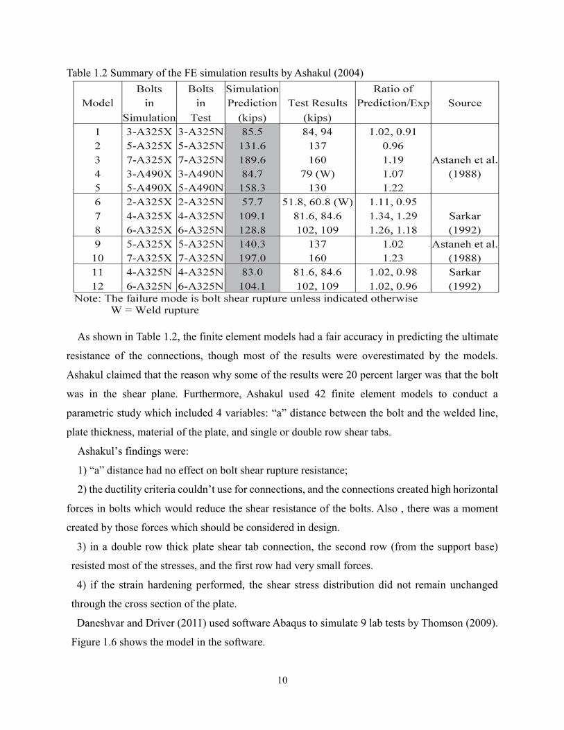
Daneshvar and Driver (2011) used software Abaqus to simulate 9 lab tests by Thomson (2009).
Figure 1.6 shows the model in the software.
11
Figure 1.6 Daneshvar and Driver’s finite element model
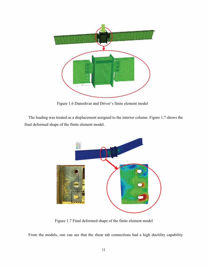
The loading was treated as a displacement assigned to the interior column. Figure 1.7 shows the
final deformed shape of the finite element model.
Figure 1.7 Final deformed shape of the finite element model
From the models, one can see that the shear tab connections had a high ductility capability
12
because of the bearing located around the bolt holes. Daneshvar and Driver concluded that the
hardest part of simulation in Abaqus was the nonlinearity definition.
Henning Levanger (2012) used software Abaqus to simulate ductile fracture in steel and
compared two models for describing local instability because of ductile fracture. The first model
used material’s true stress and strain relationship for reducing load-bearing capacity to get the
ductile fracture of the material; the other model was based on the assumed energy for forming a
crack, and reduced the load-bearing capacity by giving damage to the elements of the model.
Alireza Mirzaei and co-researchers (2014) did a series of full-scale lab tests of shear tab
connections and used Abaqus to mimic the performance of these shear tab connections. A series of
four full-scale tests were performed on shear tab connections between a W610x140 beam and a
W360x196 column, as well as a W310x60 beam and a W360x196 column. The shear tab, which
was configured as a double bolt row connection, was subjected to a combined vertical (shear) force
and axial tension along with the anticipated rotation of a typical beam-to column joint. A matching
specimen was then tested under shear and axial compression. The results from these tests and
previous shear tabs tested under gravity load alone were used in the development of a finite element
model that was capable of simulating the response of the connection under shear load and
predicting the ultimate resistance and the progression of failure. The models presented in the thesis
featured special modelling techniques and were able to predict all types of failure modes such as
bearing, net area fracture, shear yielding, flexural yielding, and weld tearing of the connections.
Next, the FE models were used to investigate the performance of shear tabs subjected to
combined shear and axial force. Shear force–axial force interaction curves were generated for
various levels of axial tension and compression force for twelve connections. At last, a design
approach was proposed which allowed practicing engineers to include the effect of any axial force
level in the design of a shear tab connection.
1.4 Design guideline for shear tab connections
The current design procedure for shear tabs in the CISC Handbook of Steel Construction (2016)
is based on the research carried out by Astaneh et al. (1989). Table 3-41 in the Handbook presents
the factored resistances of shear tabs with one vertical row of 2 to 7 bolts connected to rigid
supports (such as the flange of a W section column) or flexible supports (e.g. the web of a column
or a girder) by using E49 fillet welds and diameters ½”, ¾”, 20 mm and 22 mm A325 bolts. The
13
methodology behind the values listed in the table is as follows: 1) determine the effective
eccentricity for the bolt group based on Astaneh et al’s (1989) research; 2) find the single plane
shear resistances of the bolts used; 3) determine the thickness of the shear tab plate; and 4) choose
the weld size to fully develop the shear tab. The current Canadian approach does not cover the
usage of multiple vertical rows of bolts or the use of more than 7 bolts per row. The size and
thickness of the shear tab is also limited due to restrictions largely based on the original scope of
test specimens. It also does not address the application of an axial force on the connection.
1.5 Thesis outline
Chapter 2 presents laboratory test of 10 shear tab connections under a pure tension load. The test
design, setup, procedures and results are discussed in detail.
Chapter 3 describes the finite element modeling of the tested connection specimens using
software Abaqus 6.14. The finite element model is calibrated with the experimental results.
Chapter 4 presents a parametric study of the shear tab connections by using the finite element
model established in Chapter 3. The design parameters include tab thickness, edge distance, bolt
diameter, and the combined effect with shear force.
Chapter 5 proposes a load-deformation curve for the shear tab connections from the elastic stage
to the damage stage.
Chapter 6 states the conclusions from this research, and provides some recommendations for
future works.
14
Chapter 2 Experimental test
In this chapter, the details of the lab test of 10 shear tab connections under a pure tension load are
presented.
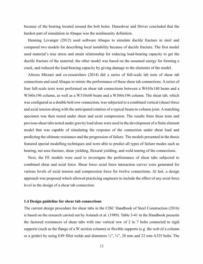
2.1 Test setup and design
The tension test was conducted on a SATEC 500 kips (2225 kN) universal testing machine. Figure
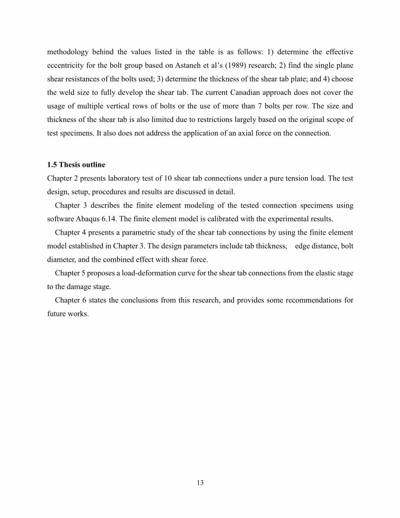
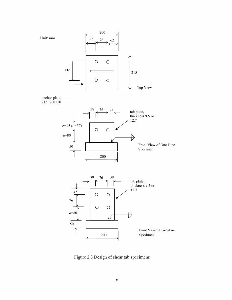
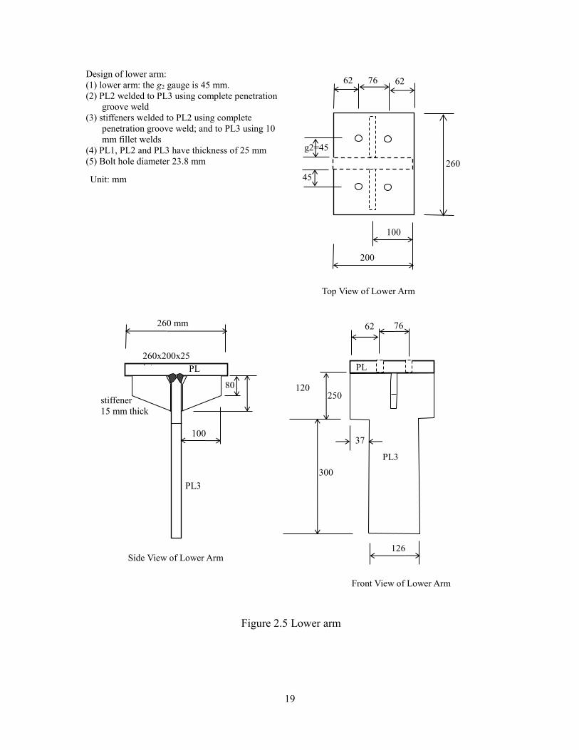
2.1 shows a picture of the setup in lab. Figure 2.2 shows the design of the setup, which consisted
of one upper loading arm, one lower loading arm, and a specimen between the loading arms. The
design of the shear tab specimen is shown in Figure 2.3. The loading arms were fixed to the loading
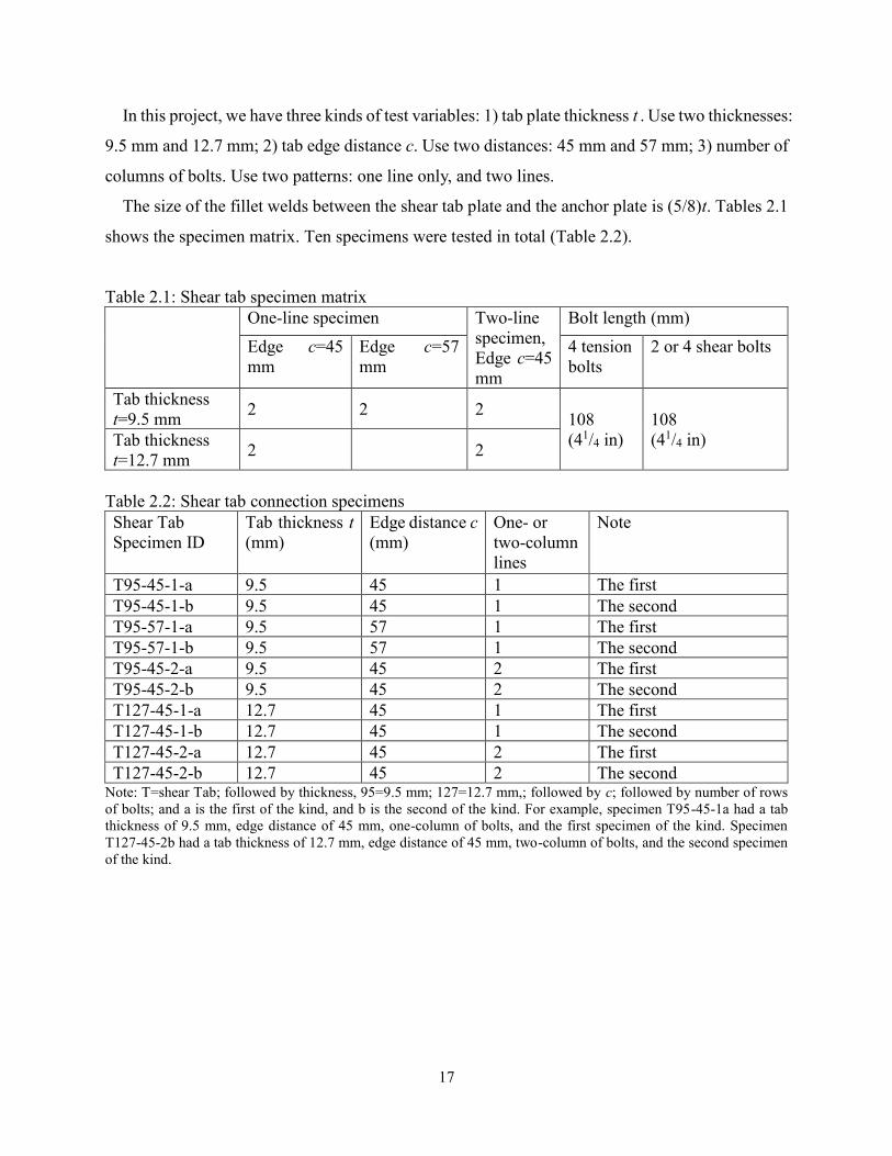
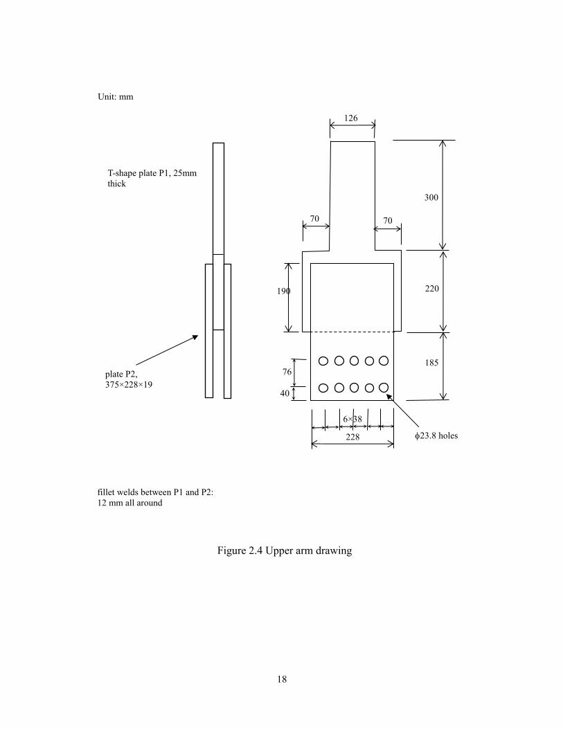
heads of the universal testing machine by clamping (Figure 2.4 and Figure 2.5). Figure 2.6 shows
the measurement of displacement.
Figure 2.1 The test setup on universal testing machine
15
Figure 2.2 Test setup for pure tension
Measurements: 1) tension force T 2) elongation Δ
lower arm
tension
50
tab plate, fillet welded to anchor plate 116
anchor plate, 50 mm thick
300
126
220
185
Unit: mm
16
anchor plate, 215×200×50
Figure 2.3 Design of shear tab specimens
215
200
116
76 62 62
tab plate, thickness 9.5 or 12.7
a=80
50
c= 45 (or 57)
200
76 38 38
Top View
Front View of One-Line Specimen
Front View of Two-Line Specimen
tab plate, thickness 9.5 or 12.7
a=80
50
45
200
76 38 38
76
Unit: mm
17
In this project, we have three kinds of test variables: 1) tab plate thickness t . Use two thicknesses:
9.5 mm and 12.7 mm; 2) tab edge distance c. Use two distances: 45 mm and 57 mm; 3) number of
columns of bolts. Use two patterns: one line only, and two lines.
The size of the fillet welds between the shear tab plate and the anchor plate is (5/8)t. Tables 2.1
shows the specimen matrix. Ten specimens were tested in total (Table 2.2).
Table 2.1: Shear tab specimen matrix One-line specimen Two-line
specimen, Edge c=45 mm
Bolt length (mm) Edge c=45 mm
Edge c=57 mm
4 tension bolts
2 or 4 shear bolts
Tab thickness t=9.5 mm 2 2 2 108
(41/4 in) 108 (41/4 in) Tab thickness
t=12.7 mm 2 2
Table 2.2: Shear tab connection specimens Shear Tab Specimen ID
Tab thickness t (mm)
Edge distance c (mm)
One- or two-column lines
Note
T95-45-1-a 9.5 45 1 The first T95-45-1-b 9.5 45 1 The second T95-57-1-a 9.5 57 1 The first T95-57-1-b 9.5 57 1 The second T95-45-2-a 9.5 45 2 The first T95-45-2-b 9.5 45 2 The second T127-45-1-a 12.7 45 1 The first T127-45-1-b 12.7 45 1 The second T127-45-2-a 12.7 45 2 The first T127-45-2-b 12.7 45 2 The second
Note: T=shear Tab; followed by thickness, 95=9.5 mm; 127=12.7 mm,; followed by c; followed by number of rows of bolts; and a is the first of the kind, and b is the second of the kind. For example, specimen T95-45-1a had a tab thickness of 9.5 mm, edge distance of 45 mm, one-column of bolts, and the first specimen of the kind. Specimen T127-45-2b had a tab thickness of 12.7 mm, edge distance of 45 mm, two-column of bolts, and the second specimen of the kind.
18
Figure 2.4 Upper arm drawing
228
70
40
fillet welds between P1 and P2: 12 mm all around
23.8 holes
plate P2, 375×228×19
300
126
220
185
70
190
6×38
76
T-shape plate P1, 25mm thick
Unit: mm
19
260 mm
260
Figure 2.5 Lower arm
300
stiffener 15 mm thick
260x200x25 plate
200
126
PL2
76 62
PL2
g2=45
45
76 62 62
100
250 120 80
100
PL3
PL3
Top View of Lower Arm
Side View of Lower Arm
Front View of Lower Arm
Design of lower arm: (1) lower arm: the g2 gauge is 45 mm. (2) PL2 welded to PL3 using complete penetration
groove weld (3) stiffeners welded to PL2 using complete
penetration groove weld; and to PL3 using 10 mm fillet welds
(4) PL1, PL2 and PL3 have thickness of 25 mm (5) Bolt hole diameter 23.8 mm
37
Unit: mm
20
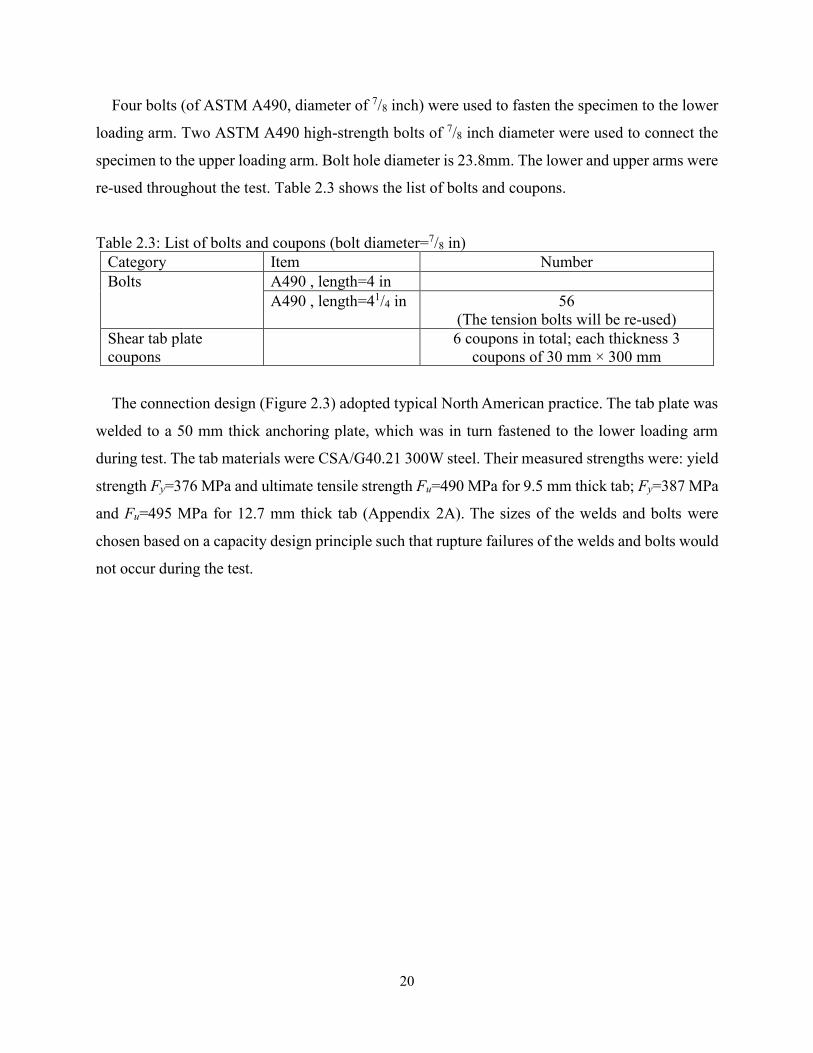
Four bolts (of ASTM A490, diameter of 7/8 inch) were used to fasten the specimen to the lower
loading arm. Two ASTM A490 high-strength bolts of 7/8 inch diameter were used to connect the
specimen to the upper loading arm. Bolt hole diameter is 23.8mm. The lower and upper arms were
re-used throughout the test. Table 2.3 shows the list of bolts and coupons.
Table 2.3: List of bolts and coupons (bolt diameter=7/8 in) Category Item Number Bolts A490 , length=4 in
A490 , length=41/4 in 56 (The tension bolts will be re-used)
Shear tab plate coupons
6 coupons in total; each thickness 3 coupons of 30 mm × 300 mm
The connection design (Figure 2.3) adopted typical North American practice. The tab plate was
welded to a 50 mm thick anchoring plate, which was in turn fastened to the lower loading arm
during test. The tab materials were CSA/G40.21 300W steel. Their measured strengths were: yield
strength Fy=376 MPa and ultimate tensile strength Fu=490 MPa for 9.5 mm thick tab; Fy=387 MPa
and Fu=495 MPa for 12.7 mm thick tab (Appendix 2A). The sizes of the welds and bolts were
chosen based on a capacity design principle such that rupture failures of the welds and bolts would
not occur during the test.
21
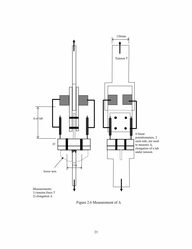
Figure 2.6 Measurement of Δ
Measurements: 1) tension force T 2) elongation Δ
lower arm
Tension T
116
g1
126mm
Δ of tab
4 linear potentiometers, 2 each side, are used to measure Δ, elongation of a tab under tension.
22
2.2 Test procedure
Before starting, measure dimensions of the test arms, check if they match design dimensions. All
the shear tab specimens shall be measured and photoed before testing. Photos shall be taken with
the tab placed on a clean background (a white color board as background). When taking photos,
always include a printed label showing the ID of the connection.
The test procedures are as follows:
1) place the lower arm onto the Universal Testing machine.
2) install shear tab specimen, and snug tighten the tension bolts.
3) place the upper loading arm. Install and snug tighten shear bolts.
4) take photos of the connection, with printed lab of ID.
5) install displacement gauges.
6) check data acquisition system.
7) set up safety screen.
8) start loading while recording data. Load the connection to rupture with displacement-
controlled loading.
9) unload.
10) take photos of the connection before taking it off, including printed label ID.
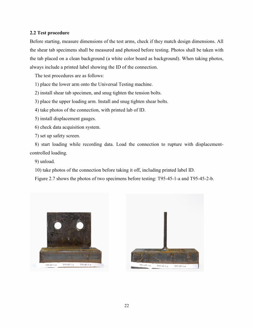
Figure 2.7 shows the photos of two specimens before testing: T95-45-1-a and T95-45-2-b.
23
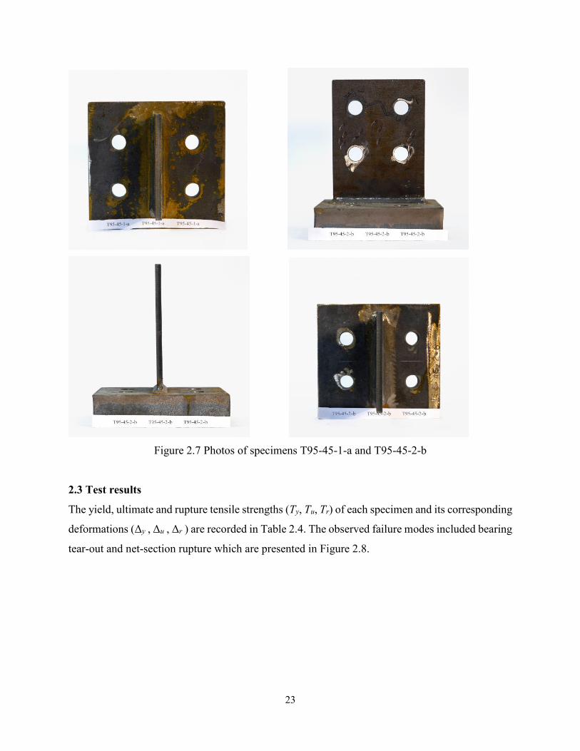
Figure 2.7 Photos of specimens T95-45-1-a and T95-45-2-b
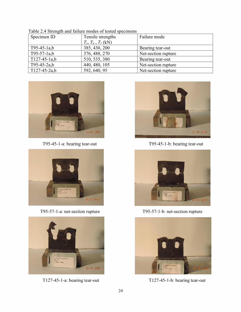
2.3 Test results
The yield, ultimate and rupture tensile strengths (Ty, Tu, Tr) of each specimen and its corresponding
deformations (Δy , Δu , Δr ) are recorded in Table 2.4. The observed failure modes included bearing
tear-out and net-section rupture which are presented in Figure 2.8.
24
Table 2.4 Strength and failure modes of tested specimens Specimen ID Tensile strengths
Ty, Tu , Tr (kN) Failure mode
T95-45-1a,b 385, 430, 200 Bearing tear-out T95-57-1a,b 376, 488, 270 Net-section rupture T127-45-1a,b 510, 535, 380 Bearing tear-out T95-45-2a,b 440, 480, 105 Net-section rupture T127-45-2a,b 592, 640, 95 Net-section rupture
T95-45-1-a: bearing tear-out T95-45-1-b: bearing tear-out
T95-57-1-a: net-section rupture T95-57-1-b: net-section rupture
T127-45-1-a: bearing tear-out T127-45-1-b: bearing tear-out
25
T95-45-2-a: net-section rupture T95-45-2-b: net-section rupture
T127-45-2-a: net-section rupture T127-45-2-b: net-section rupture
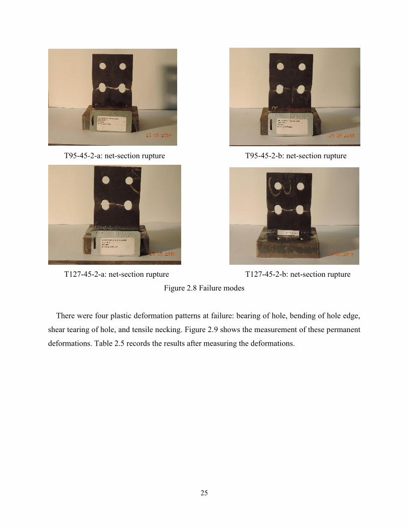
Figure 2.8 Failure modes
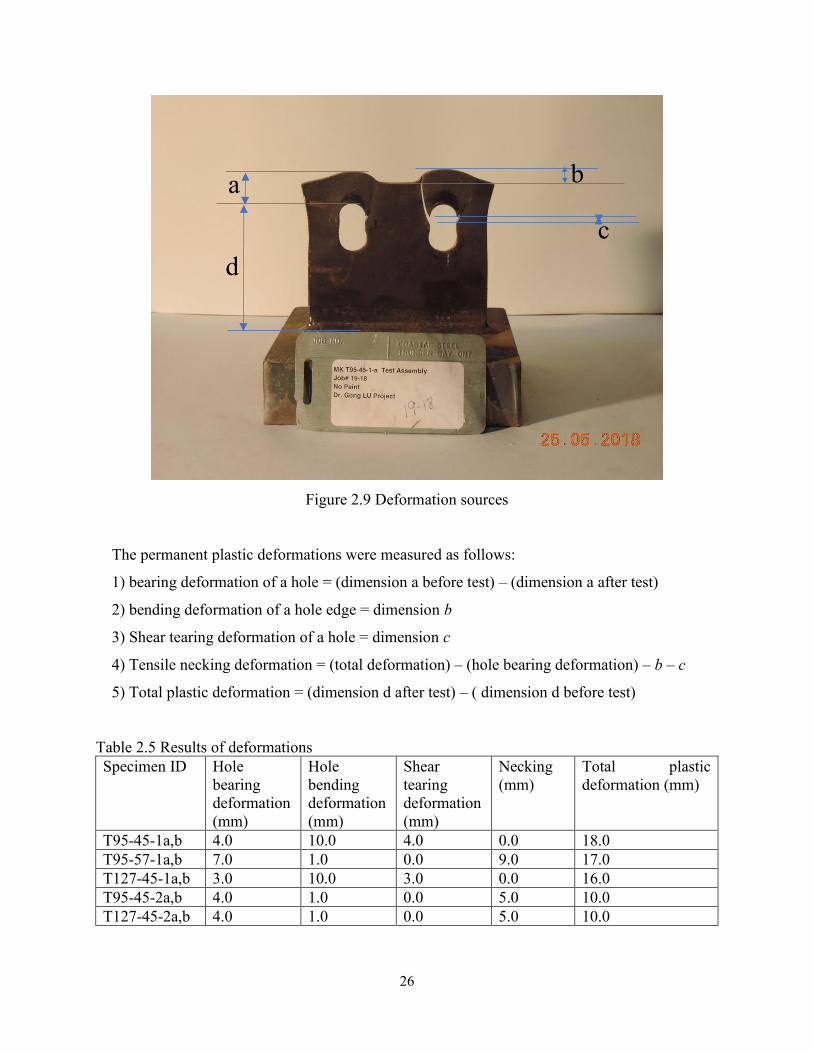
There were four plastic deformation patterns at failure: bearing of hole, bending of hole edge,
shear tearing of hole, and tensile necking. Figure 2.9 shows the measurement of these permanent
deformations. Table 2.5 records the results after measuring the deformations.
26
Figure 2.9 Deformation sources
The permanent plastic deformations were measured as follows:
1) bearing deformation of a hole = (dimension a before test) – (dimension a after test)
2) bending deformation of a hole edge = dimension b
3) Shear tearing deformation of a hole = dimension c
4) Tensile necking deformation = (total deformation) – (hole bearing deformation) – b – c
5) Total plastic deformation = (dimension d after test) – ( dimension d before test)
Table 2.5 Results of deformations Specimen ID Hole
bearing deformation (mm)
Hole bending deformation (mm)
Shear tearing deformation (mm)
Necking (mm)
Total plastic deformation (mm)
T95-45-1a,b 4.0 10.0 4.0 0.0 18.0 T95-57-1a,b 7.0 1.0 0.0 9.0 17.0 T127-45-1a,b 3.0 10.0 3.0 0.0 16.0 T95-45-2a,b 4.0 1.0 0.0 5.0 10.0 T127-45-2a,b 4.0 1.0 0.0 5.0 10.0
a
d
b
c
27
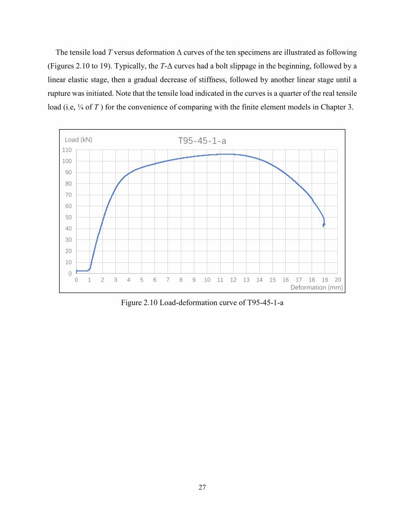
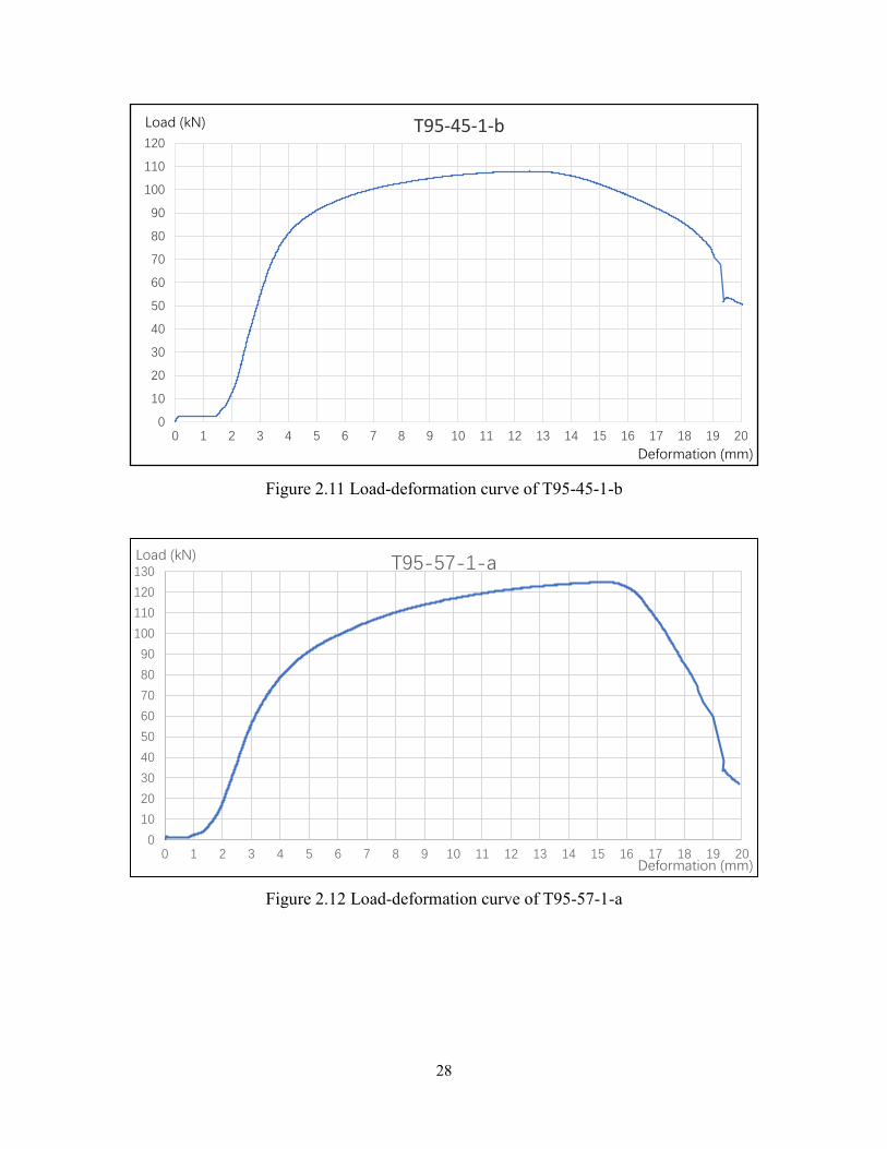
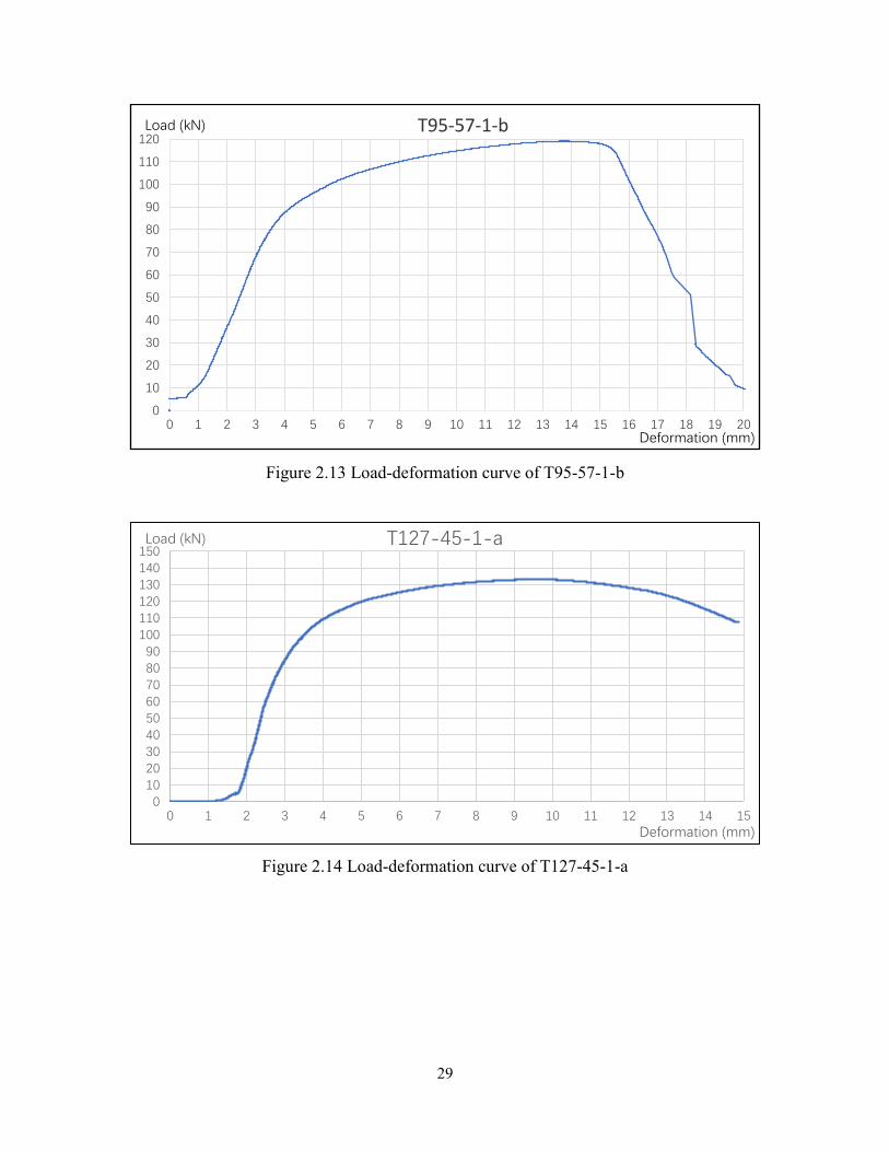
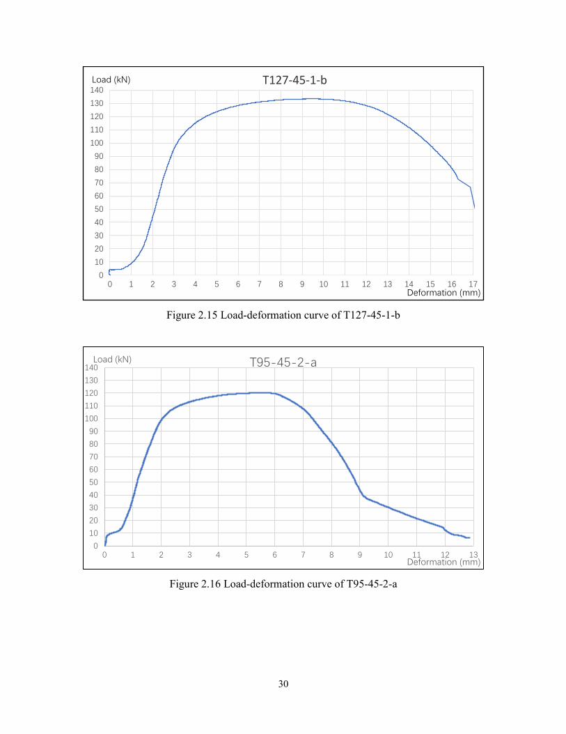
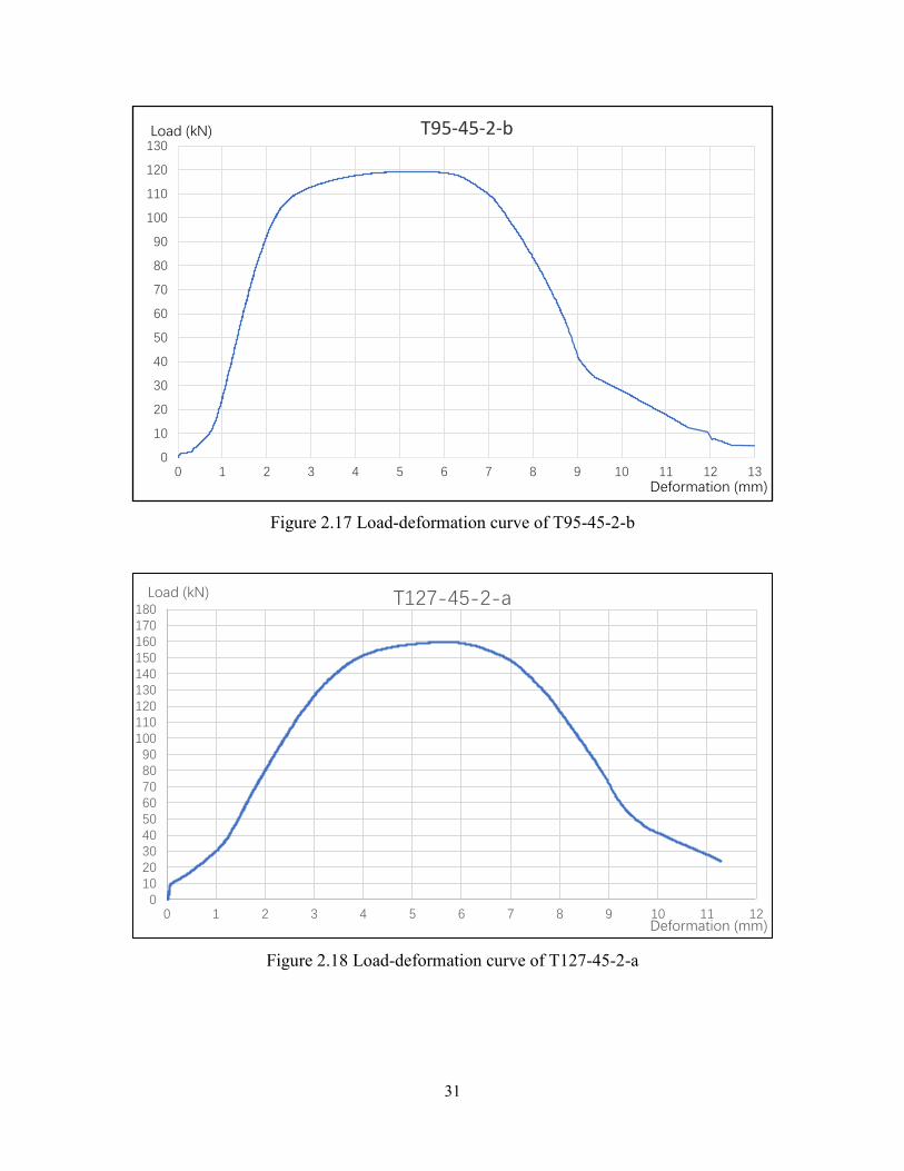
The tensile load T versus deformation Δ curves of the ten specimens are illustrated as following
(Figures 2.10 to 19). Typically, the T-Δ curves had a bolt slippage in the beginning, followed by a
linear elastic stage, then a gradual decrease of stiffness, followed by another linear stage until a
rupture was initiated. Note that the tensile load indicated in the curves is a quarter of the real tensile
load (i.e, ¼ of T ) for the convenience of comparing with the finite element models in Chapter 3.
Figure 2.10 Load-deformation curve of T95-45-1-a
0
10
20
30
40
50
60
70
80
90
100
110
0 1 2 3 4 5 6 7 8 9 10 11 12 13 14 15 16 17 18 19 20
Load (kN)
Deformation (mm)
T95-45-1-a
28
Figure 2.11 Load-deformation curve of T95-45-1-b
Figure 2.12 Load-deformation curve of T95-57-1-a
0
10
20
30
40
50
60
70
80
90
100
110
120
0 1 2 3 4 5 6 7 8 9 10 11 12 13 14 15 16 17 18 19 20
Load (kN)
Deformation (mm)
T95-45-1-b
0
10
20
30
40
50
60
70
80
90
100
110
120
130
0 1 2 3 4 5 6 7 8 9 10 11 12 13 14 15 16 17 18 19 20
Load (kN)
Deformation (mm)
T95-57-1-a
29
Figure 2.13 Load-deformation curve of T95-57-1-b
Figure 2.14 Load-deformation curve of T127-45-1-a
0
10
20
30
40
50
60
70
80
90
100
110
120
0 1 2 3 4 5 6 7 8 9 10 11 12 13 14 15 16 17 18 19 20
Load (kN)
Deformation (mm)
T95-57-1-b
0102030405060708090
100110120130140150
0 1 2 3 4 5 6 7 8 9 10 11 12 13 14 15
Load (kN)
Deformation (mm)
T127-45-1-a
30
Figure 2.15 Load-deformation curve of T127-45-1-b
Figure 2.16 Load-deformation curve of T95-45-2-a
0
10
20
30
40
50
60
70
80
90
100
110
120
130
140
0 1 2 3 4 5 6 7 8 9 10 11 12 13 14 15 16 17
Load (kN)
Deformation (mm)
T127-45-1-b
0
10
20
30
40
50
60
70
80
90
100
110
120
130
140
0 1 2 3 4 5 6 7 8 9 10 11 12 13
Load (kN)
Deformation (mm)
T95-45-2-a
31
Figure 2.17 Load-deformation curve of T95-45-2-b
Figure 2.18 Load-deformation curve of T127-45-2-a
0
10
20
30
40
50
60
70
80
90
100
110
120
130
0 1 2 3 4 5 6 7 8 9 10 11 12 13
Load (kN)
Deformation (mm)
T95-45-2-b
0102030405060708090
100110120130140150160170180
0 1 2 3 4 5 6 7 8 9 10 11 12
Load (kN)
Deformation (mm)
T127-45-2-a
32
Figure 2.19 Load-deformation curve of T127-45-2-b
0
10
20
30
40
50
60
70
80
90
100
110
120
130
140
150
160
170
0 1 2 3 4 5 6 7 8 9 10 11 12
Load (kN)
Deformation (mm)
T127-45-2-b
33
2A Appendix Coupon test
Tensile coupon tests were used to determine the material’s yield strength, ultimate strength, and
fracture strain. In this study, tensile coupon tests were carried out using Tinius Olsen universal
testing machine.
The coupons (300mm 30mm) were cut from the shear tab plates. The specified material for
shear tab plates was G40.21 300W steel.
Three coupons were cut for 9.5mm thickness tab and 12.7mm thickness tab, respectively. Figure
2.20 shows the dimensions of the coupons.
Test Procedure:
1) measure the length and thickness of the coupons
2) install the coupons to Tinius Olsen universal testing machine
3) install the gauges on the coupon
4) input the essential parameters to the computer
5) start recording data
6) start loading to rupture
7) unload
8) measure the length and thickness of the coupons
Figure 2.21 shows the testing machine with a coupon on it and the coupons after test.
78.7mm
300 mm
Figure 2.20 Coupon size

34
Figure 2.21 Coupon setup and photos after test
The thickness, middle length before and after testing of each coupon were recorded in Table 2.6.
Table 2.6 Measurement of each coupon Coupon ID Thickness (mm) Middle length
(mm) Middle length after test (mm)
elongation
Coupon 1 12.31 7.87 9.87 0.25 Coupon 3 12.29 7.87 9.74 0.24 Coupon 4 9.32 7.87 9.88 0.25 Coupon 5 9.34 7.87 9.81 0.25 Coupon 6 9.42 7.87 9.88 0.26
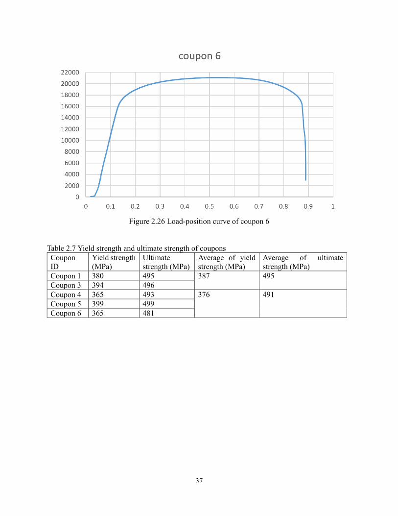
The load versus position curves of each coupon are given as Figures 2.22 to 26 (unit: lbf, in).
The yielding strength and ultimate strength of each coupon can be obtained from the load vs.
position curves (Table 2.7).
35
Figure 2.22 Load-position curve of coupon 1
Figure 2.23 Load-position curve of coupon 3
36
Figure 2.24 Load-position curve of coupon 4
Figure 2.25 Load-position curve of coupon 5
37
Figure 2.26 Load-position curve of coupon 6
Table 2.7 Yield strength and ultimate strength of coupons Coupon ID
Yield strength (MPa)
Ultimate strength (MPa)
Average of yield strength (MPa)
Average of ultimate strength (MPa)
Coupon 1 380 495 387 495 Coupon 3 394 496 Coupon 4 365 493 376 491 Coupon 5 399 499 Coupon 6 365 481
38
Chapter 3 Finite element modeling
This chapter describes the finite element modeling of the tested specimens, using software Abaqus
6.14. In a finite element analysis, a shear tab is discretized into many small elements, and the
displacements at each node and the stresses within every element are obtained under the applied
load.
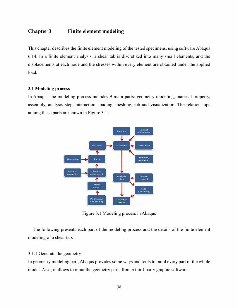
3.1 Modeling process
In Abaqus, the modeling process includes 9 main parts: geometry modeling, material property,
assembly, analysis step, interaction, loading, meshing, job and visualization. The relationships
among these parts are shown in Figure 3.1.
Figure 3.1 Modeling process in Abaqus
The following presents each part of the modeling process and the details of the finite element
modeling of a shear tab.
3.1.1 Generate the geometry
In geometry modeling part, Abaqus provides some ways and tools to build every part of the whole
model. Also, it allows to input the geometry parts from a third-party graphic software.
39
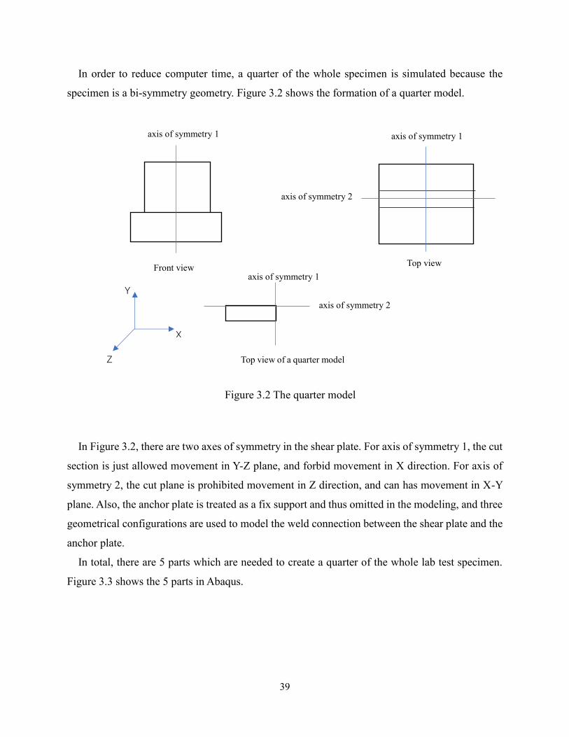
In order to reduce computer time, a quarter of the whole specimen is simulated because the
specimen is a bi-symmetry geometry. Figure 3.2 shows the formation of a quarter model.
In Figure 3.2, there are two axes of symmetry in the shear plate. For axis of symmetry 1, the cut
section is just allowed movement in Y-Z plane, and forbid movement in X direction. For axis of
symmetry 2, the cut plane is prohibited movement in Z direction, and can has movement in X-Y
plane. Also, the anchor plate is treated as a fix support and thus omitted in the modeling, and three
geometrical configurations are used to model the weld connection between the shear plate and the
anchor plate.
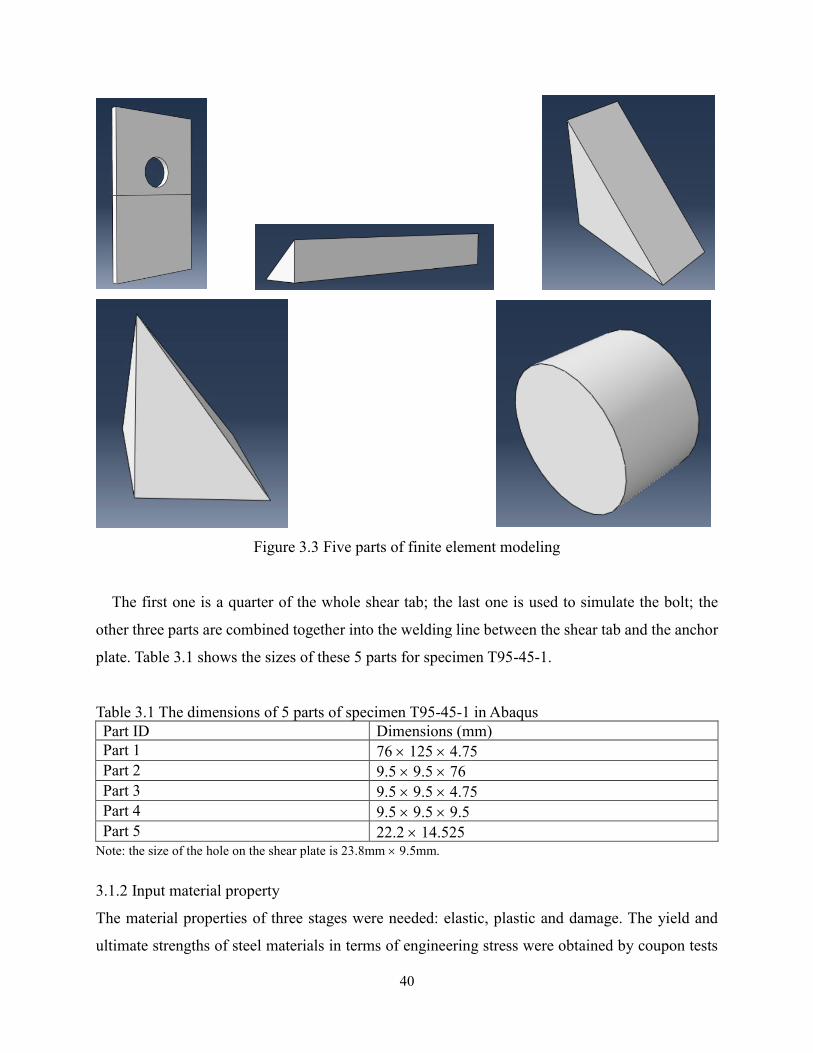
In total, there are 5 parts which are needed to create a quarter of the whole lab test specimen.
Figure 3.3 shows the 5 parts in Abaqus.
axis of symmetry 1
axis of symmetry 2
axis of symmetry 1
axis of symmetry 2
Figure 3.2 The quarter model
Top view Front view
Top view of a quarter model
axis of symmetry 1
X
Y
Z
40
Figure 3.3 Five parts of finite element modeling
The first one is a quarter of the whole shear tab; the last one is used to simulate the bolt; the
other three parts are combined together into the welding line between the shear tab and the anchor
plate. Table 3.1 shows the sizes of these 5 parts for specimen T95-45-1.
Table 3.1 The dimensions of 5 parts of specimen T95-45-1 in Abaqus Part ID Dimensions (mm) Part 1 76 125 4.75 Part 2 9.5 9.5 76 Part 3 9.5 9.5 4.75 Part 4 9.5 9.5 9.5 Part 5 22.2 14.525
Note: the size of the hole on the shear plate is 23.8mm 9.5mm.
3.1.2 Input material property
The material properties of three stages were needed: elastic, plastic and damage. The yield and
ultimate strengths of steel materials in terms of engineering stress were obtained by coupon tests
41
(see 2A appendix for details).
In elastic stage, 200 GPa and 0.3 for Young’s Modulus and Poisson’s ratio were used. In plastic
stage, the stress and strain are required to be expressed as the true stress and strain instead of
engineering stress and strain. The relationships between true strain, stress and engineering strain,
stress are as follows:
= E (1 + E) (3.1)
and
= ln(1 + E) (3.2)
where and are true strain and stress, respectively; E and E are engineering strain and stress,
respectively.
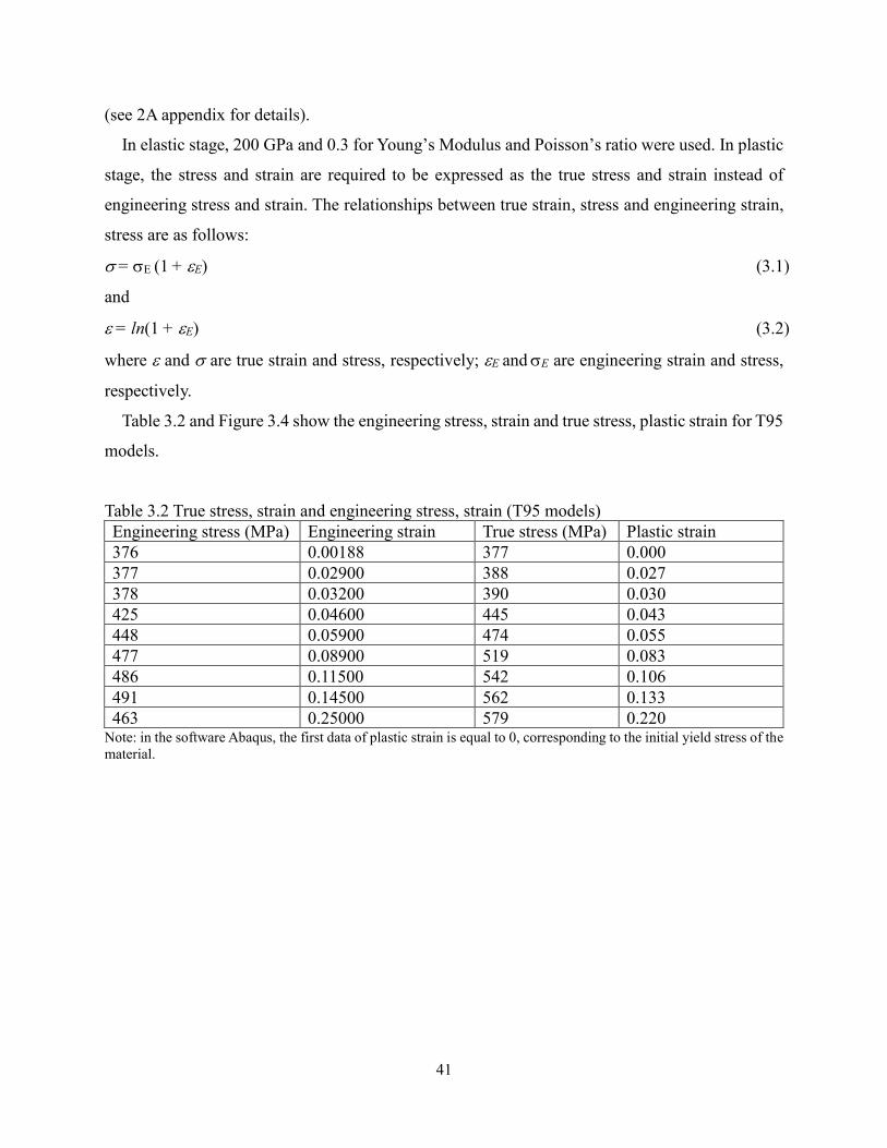
Table 3.2 and Figure 3.4 show the engineering stress, strain and true stress, plastic strain for T95
models.
Table 3.2 True stress, strain and engineering stress, strain (T95 models) Engineering stress (MPa) Engineering strain True stress (MPa) Plastic strain 376 0.00188 377 0.000 377 0.02900 388 0.027 378 0.03200 390 0.030 425 0.04600 445 0.043 448 0.05900 474 0.055 477 0.08900 519 0.083 486 0.11500 542 0.106 491 0.14500 562 0.133 463 0.25000 579 0.220
Note: in the software Abaqus, the first data of plastic strain is equal to 0, corresponding to the initial yield stress of the material.
42
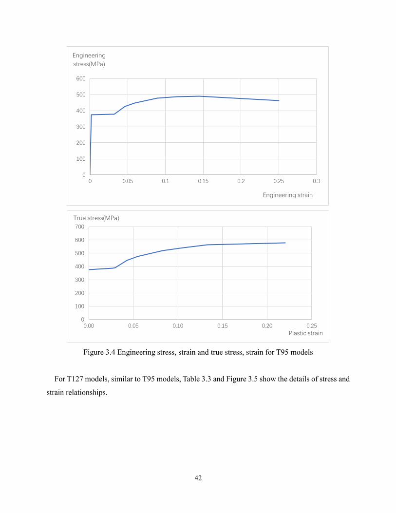
Figure 3.4 Engineering stress, strain and true stress, strain for T95 models
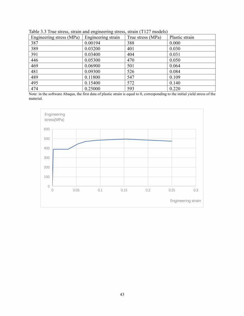
For T127 models, similar to T95 models, Table 3.3 and Figure 3.5 show the details of stress and
strain relationships.
0
100
200
300
400
500
600
0 0.05 0.1 0.15 0.2 0.25 0.3
Engineering
stress(MPa)
Engineering strain
0
100
200
300
400
500
600
700
0.00 0.05 0.10 0.15 0.20 0.25
True stress(MPa)
Plastic strain
43
Table 3.3 True stress, strain and engineering stress, strain (T127 models) Engineering stress (MPa) Engineering strain True stress (MPa) Plastic strain 387 0.00194 388 0.000 389 0.03200 401 0.030 391 0.03400 404 0.031 446 0.05300 470 0.050 469 0.06900 501 0.064 481 0.09300 526 0.084 489 0.11800 547 0.109 495 0.15400 572 0.140 474 0.25000 593 0.220
Note: in the software Abaqus, the first data of plastic strain is equal to 0, corresponding to the initial yield stress of the material.
0
100
200
300
400
500
600
0 0.05 0.1 0.15 0.2 0.25 0.3
Engineering
stress(MPa)
Engineering strain
44
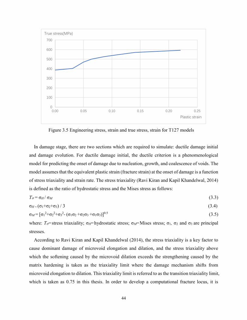
Figure 3.5 Engineering stress, strain and true stress, strain for T127 models
In damage stage, there are two sections which are required to simulate: ductile damage initial
and damage evolution. For ductile damage initial, the ductile criterion is a phenomenological
model for predicting the onset of damage due to nucleation, growth, and coalescence of voids. The
model assumes that the equivalent plastic strain (fracture strain) at the onset of damage is a function
of stress triaxiality and strain rate. The stress triaxiality (Ravi Kiran and Kapil Khandelwal, 2014)
is defined as the ratio of hydrostatic stress and the Mises stress as follows:
T = σH / σM (3.3)
σH = (σ1+σ2+σ3) / 3 (3.4)
σM = [σ12+σ2
2+σ32- (σ1σ2 +σ2σ3 +σ1σ3)]0.5 (3.5)
where: T=stress triaxiality; σH=hydrostatic stress; σM=Mises stress; σ1, σ2 and σ3 are principal
stresses.
According to Ravi Kiran and Kapil Khandelwal (2014), the stress triaxiality is a key factor to
cause dominant damage of microvoid elongation and dilation, and the stress triaxiality above
which the softening caused by the microvoid dilation exceeds the strengthening caused by the
matrix hardening is taken as the triaxiality limit where the damage mechanism shifts from
microvoid elongation to dilation. This triaxiality limit is referred to as the transition triaxiality limit,
which is taken as 0.75 in this thesis. In order to develop a computational fracture locus, it is
0
100
200
300
400
500
600
700
0.00 0.05 0.10 0.15 0.20 0.25
True stress(MPa)
Plastic strain
45
assumed that microvoid elongation and dilation are the only mechanisms of damage at low (less
than the transition triaxiality limit) and high triaxiality (larger than the transition triaxiality limit),
respectively.
For the low triaxiality regime (T ranges from zero to the transition limit), it is assumed that the
void elongation ratio reaches a critical value before the ligament between two neighboring
elongated microvoid fails (causing a local material to fracture). The critical value of void
elongation ratio is taken as 4 in this thesis.
For the high stress triaxiality regime, a rapid microvoid growth is observed at a certain
macroscopic effective plastic strain value. At this strain, the softening due to rapid microvoid
dilation dominates the matrix hardening leading to strain localization in the intervoid ligaments
resulting in overall softening behavior and finally leading to local material fracture.
In other words, for the fracture locus, in the low triaxiality regime the fracture strain increases
with the increase in triaxiality because the tendency of microvoids to elongate decreases with the
increase of the stress triaxiality. For high regime, the fracture strain decreases rapidly with the
increase of the stress triaxiality due to the fact that microvoids dilate rapidly at the high stress
triaxiality.
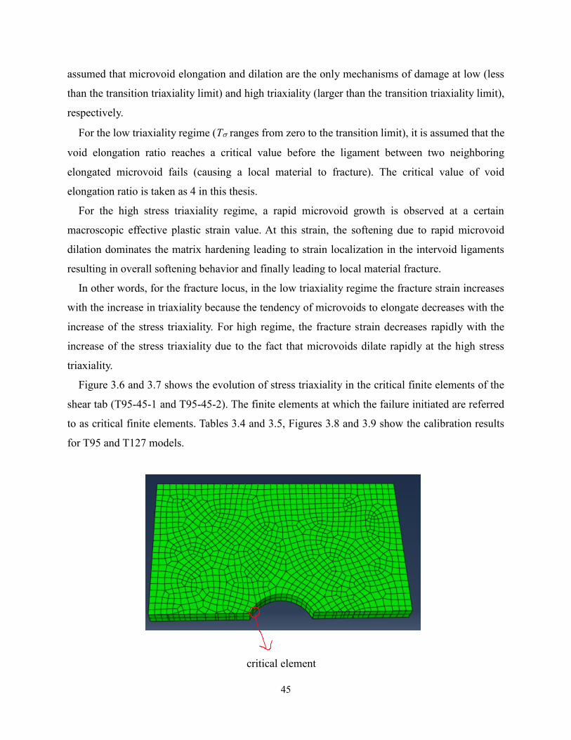
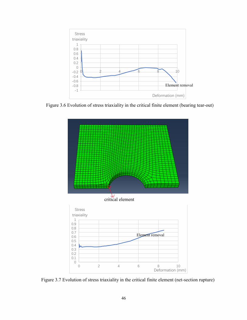
Figure 3.6 and 3.7 shows the evolution of stress triaxiality in the critical finite elements of the
shear tab (T95-45-1 and T95-45-2). The finite elements at which the failure initiated are referred
to as critical finite elements. Tables 3.4 and 3.5, Figures 3.8 and 3.9 show the calibration results
for T95 and T127 models.
critical element
46
Figure 3.6 Evolution of stress triaxiality in the critical finite element (bearing tear-out)
critical element
Figure 3.7 Evolution of stress triaxiality in the critical finite element (net-section rupture)
-1-0.8-0.6-0.4-0.2
00.20.40.60.8
1
0 2 4 6 8 10
Stress
triaxiality
Deformation (mm)
00.10.20.30.40.50.60.70.80.9
1
0 2 4 6 8 10
Stress
triaxiality
Deformation (mm)
Element removal
Element removal
47
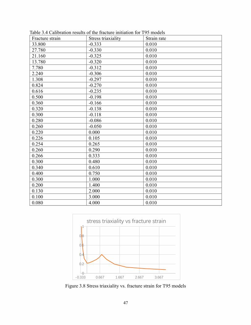
Table 3.4 Calibration results of the fracture initiation for T95 models Fracture strain Stress triaxiality Strain rate 33.800 -0.333 0.010 27.780 -0.330 0.010 21.160 -0.325 0.010 13.780 -0.320 0.010 7.780 -0.312 0.010 2.240 -0.306 0.010 1.308 -0.297 0.010 0.824 -0.270 0.010 0.616 -0.235 0.010 0.500 -0.198 0.010 0.360 -0.166 0.010 0.320 -0.138 0.010 0.300 -0.118 0.010 0.280 -0.086 0.010 0.260 -0.050 0.010 0.220 0.000 0.010 0.226 0.105 0.010 0.254 0.265 0.010 0.260 0.290 0.010 0.266 0.333 0.010 0.300 0.480 0.010 0.340 0.610 0.010 0.400 0.750 0.010 0.300 1.000 0.010 0.200 1.400 0.010 0.130 2.000 0.010 0.100 3.000 0.010 0.080 4.000 0.010
Figure 3.8 Stress triaxiality vs. fracture strain for T95 models
0
0.2
0.4
0.6
0.8
1
-0.333 0.667 1.667 2.667 3.667
stress triaxiality vs fracture strain
48
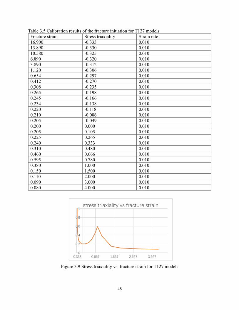
Table 3.5 Calibration results of the fracture initiation for T127 models Fracture strain Stress triaxiality Strain rate 16.900 -0.333 0.010 13.890 -0.330 0.010 10.580 -0.325 0.010 6.890 -0.320 0.010 3.890 -0.312 0.010 1.120 -0.306 0.010 0.654 -0.297 0.010 0.412 -0.270 0.010 0.308 -0.235 0.010 0.265 -0.198 0.010 0.245 -0.166 0.010 0.234 -0.138 0.010 0.220 -0.118 0.010 0.210 -0.086 0.010 0.205 -0.049 0.010 0.200 0.000 0.010 0.205 0.105 0.010 0.225 0.265 0.010 0.240 0.333 0.010 0.310 0.480 0.010 0.460 0.666 0.010 0.595 0.780 0.010 0.380 1.000 0.010 0.150 1.500 0.010 0.110 2.000 0.010 0.090 3.000 0.010 0.080 4.000 0.010
Figure 3.9 Stress triaxiality vs. fracture strain for T127 models
0
0.2
0.4
0.6
0.8
1
-0.333 0.667 1.667 2.667 3.667
stress triaxiality vs fracture strain
49
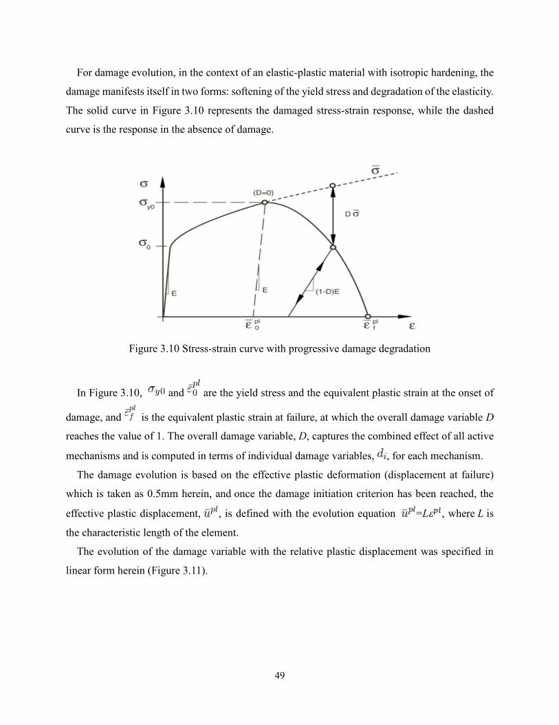
For damage evolution, in the context of an elastic-plastic material with isotropic hardening, the
damage manifests itself in two forms: softening of the yield stress and degradation of the elasticity.
The solid curve in Figure 3.10 represents the damaged stress-strain response, while the dashed
curve is the response in the absence of damage.
Figure 3.10 Stress-strain curve with progressive damage degradation
In Figure 3.10, and are the yield stress and the equivalent plastic strain at the onset of
damage, and is the equivalent plastic strain at failure, at which the overall damage variable D
reaches the value of 1. The overall damage variable, D, captures the combined effect of all active
mechanisms and is computed in terms of individual damage variables, , for each mechanism.
The damage evolution is based on the effective plastic deformation (displacement at failure)
which is taken as 0.5mm herein, and once the damage initiation criterion has been reached, the
effective plastic displacement, , is defined with the evolution equation =L𝑝𝑙, where L is
the characteristic length of the element.
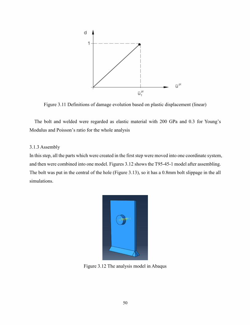
The evolution of the damage variable with the relative plastic displacement was specified in
linear form herein (Figure 3.11).
50
Figure 3.11 Definitions of damage evolution based on plastic displacement (linear)
The bolt and welded were regarded as elastic material with 200 GPa and 0.3 for Young’s
Modulus and Poisson’s ratio for the whole analysis
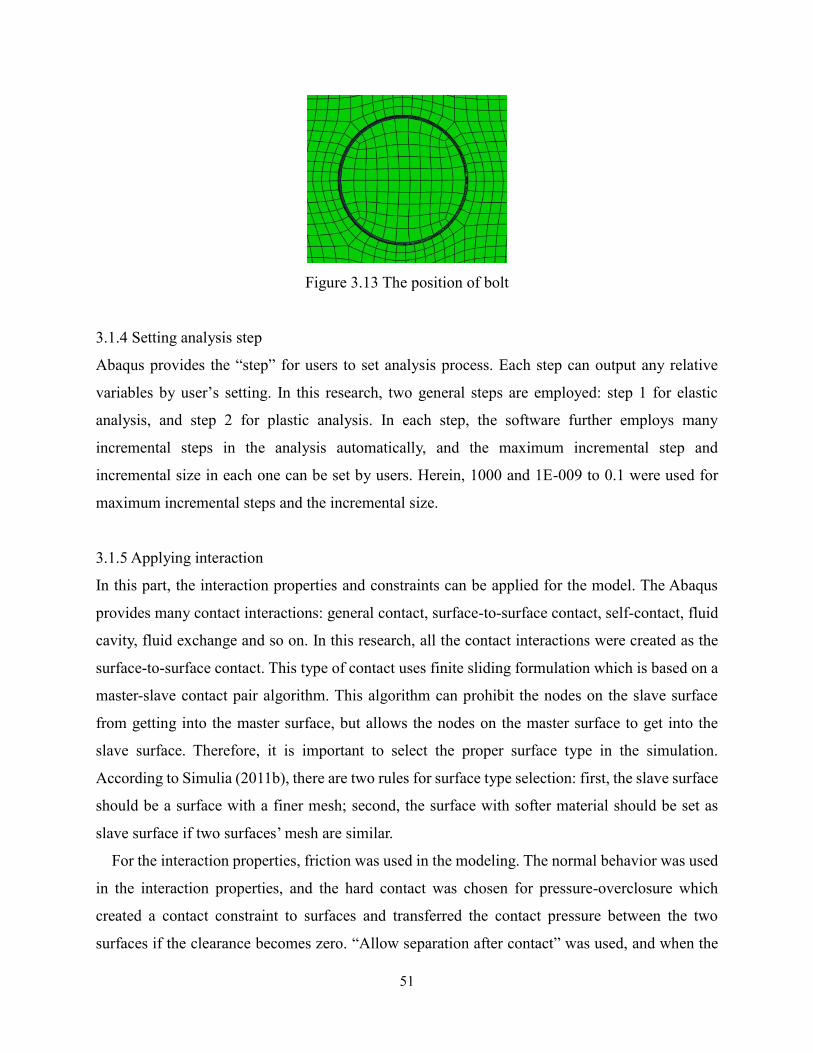
3.1.3 Assembly
In this step, all the parts which were created in the first step were moved into one coordinate system,
and then were combined into one model. Figures 3.12 shows the T95-45-1 model after assembling.
The bolt was put in the central of the hole (Figure 3.13), so it has a 0.8mm bolt slippage in the all
simulations.
Figure 3.12 The analysis model in Abaqus
51
Figure 3.13 The position of bolt
3.1.4 Setting analysis step
Abaqus provides the “step” for users to set analysis process. Each step can output any relative
variables by user’s setting. In this research, two general steps are employed: step 1 for elastic
analysis, and step 2 for plastic analysis. In each step, the software further employs many
incremental steps in the analysis automatically, and the maximum incremental step and
incremental size in each one can be set by users. Herein, 1000 and 1E-009 to 0.1 were used for
maximum incremental steps and the incremental size.
3.1.5 Applying interaction
In this part, the interaction properties and constraints can be applied for the model. The Abaqus
provides many contact interactions: general contact, surface-to-surface contact, self-contact, fluid
cavity, fluid exchange and so on. In this research, all the contact interactions were created as the
surface-to-surface contact. This type of contact uses finite sliding formulation which is based on a
master-slave contact pair algorithm. This algorithm can prohibit the nodes on the slave surface
from getting into the master surface, but allows the nodes on the master surface to get into the
slave surface. Therefore, it is important to select the proper surface type in the simulation.
According to Simulia (2011b), there are two rules for surface type selection: first, the slave surface
should be a surface with a finer mesh; second, the surface with softer material should be set as
slave surface if two surfaces’ mesh are similar.
For the interaction properties, friction was used in the modeling. The normal behavior was used
in the interaction properties, and the hard contact was chosen for pressure-overclosure which
created a contact constraint to surfaces and transferred the contact pressure between the two
surfaces if the clearance becomes zero. “Allow separation after contact” was used, and when the
52
contact pressure becomes zero or negative, this hard contact constraint was removed. The
tangential behavior was used with penalty friction formulation. This friction type controls the shear
stress transformation between the two surfaces. The tangential behavior occurred when the shear
stress reached a certain value and the slip appears between the two surfaces. Herein, the friction
coefficient was taken as 0.3.
The following three contacts with friction were used in the model:
1) the contact between the bolt surface and hole surface
2) the contact between the shear tab plate and the weld parts
3) the contact between the weld parts
For the constraint, “tie” and “coupling” were used in the modeling: the “tie” constraints were
for the surfaces of weld parts and shear plate, and the “coupling” was for the central point of the
circle surface of the bolt.
3.1.6 Applying load
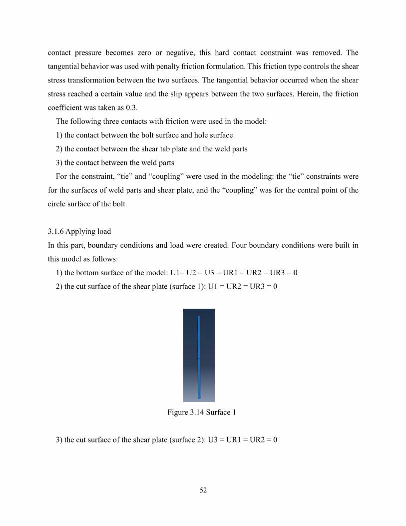
In this part, boundary conditions and load were created. Four boundary conditions were built in
this model as follows:
1) the bottom surface of the model: U1= U2 = U3 = UR1 = UR2 = UR3 = 0
2) the cut surface of the shear plate (surface 1): U1 = UR2 = UR3 = 0
Figure 3.14 Surface 1
3) the cut surface of the shear plate (surface 2): U3 = UR1 = UR2 = 0
53
Figure 3.15 Surface 2
4) the cut surface of the bolt: U3 = UR1 = UR2 = 0
For the load, a displacement load was applied to the central point of the circle surface of the bolt
and acted on the coupling point which was created in the interaction part.
3.1.7 Mesh design
Mesh design is critical in the modelling, because it has major influence on the analysis results.
The first step of meshing was to partition each individual part, because the Abaqus could not fix
the complex geometry models. Then applying the seeds was used to determine the element size.
Next, choose the proper element type for each part. Last, choose the mesh type for meshing. Table
3.6 shows the details of meshing in each part.
Table 3.6 Mesh design of each part Part ID Element
code Shape Order Nodes
Size (mm)
Part 1 C3D8R Hexahedral Linear 8 2 Part 2 C3D8R Hexahedral Linear 8 2 Part 3 C3D8R Hexahedral Linear 8 2 Part 4 C3D4H Tetrahedron Linear 4 2 Part 5 C3D8R Hexahedral Linear 8 2
Note that for the element size, 4 mm was used at first to do the modeling, but the analysis results could not converge. Then, a smaller element size of 2 mm was used for modeling, and it gave a better result (computational time between 15-20 mins). For comparison, 1 mm element size was also used for modeling, and it had the same failure mode and similar load-deformation curve as the 2 mm element size model (but computational time was more than one hour). Therefore, 2 mm element size was chosen as the final element size for modeling.
3.1.8 Job
After all the defining parts, use “job” part to do the analysis, and it provides real time monitoring
during the analyzing.
54
3.1.9 Visualization
This part provides the display of the model and analysis results. Also, any variables and other result
information which are needed can be outputted in this section.
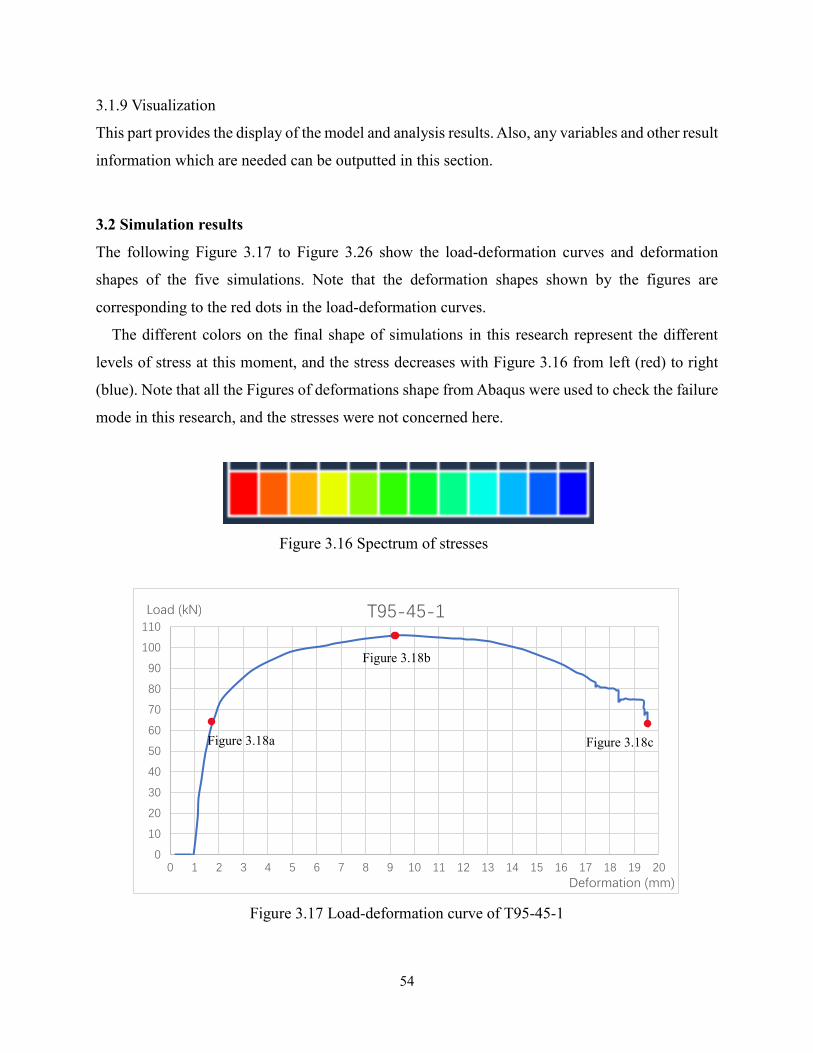
3.2 Simulation results
The following Figure 3.17 to Figure 3.26 show the load-deformation curves and deformation
shapes of the five simulations. Note that the deformation shapes shown by the figures are
corresponding to the red dots in the load-deformation curves.
The different colors on the final shape of simulations in this research represent the different
levels of stress at this moment, and the stress decreases with Figure 3.16 from left (red) to right
(blue). Note that all the Figures of deformations shape from Abaqus were used to check the failure
mode in this research, and the stresses were not concerned here.
Figure 3.16 Spectrum of stresses
Figure 3.17 Load-deformation curve of T95-45-1
0
10
20
30
40
50
60
70
80
90
100
110
0 1 2 3 4 5 6 7 8 9 10 11 12 13 14 15 16 17 18 19 20
Load (kN)
Deformation (mm)
T95-45-1
Figure 3.18a
Figure 3.18b
Figure 3.18c
55
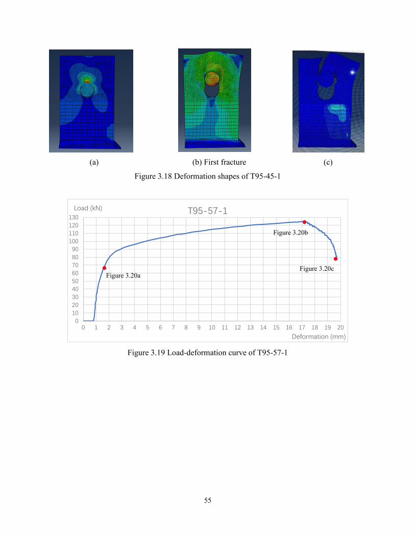
(a) (b) First fracture (c)
Figure 3.18 Deformation shapes of T95-45-1
Figure 3.19 Load-deformation curve of T95-57-1
0
10
20
30
40
50
60
70
80
90
100
110
120
130
0 1 2 3 4 5 6 7 8 9 10 11 12 13 14 15 16 17 18 19 20
Load (kN)
Deformation (mm)
T95-57-1
Figure 3.20b
Figure 3.20a Figure 3.20c
56
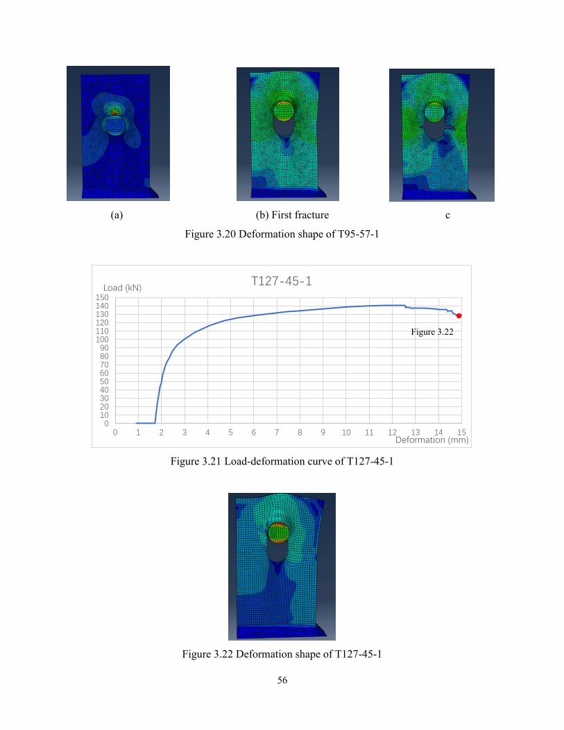
(a) (b) First fracture c
Figure 3.20 Deformation shape of T95-57-1
Figure 3.21 Load-deformation curve of T127-45-1
Figure 3.22 Deformation shape of T127-45-1
0102030405060708090
100110120130140150
0 1 2 3 4 5 6 7 8 9 10 11 12 13 14 15
Load (kN)
Deformation (mm)
T127-45-1
Figure 3.22
57
Figure 3.23 Load-deformation curve of T95-45-2
Figure 3.24 Deformation shape of T95-45-2
0102030405060708090
100110120130140
0 1 2 3 4 5 6 7 8 9 10 11 12 13
Load (kN)
Deformation (mm)
T95-45-2
Figure 3.24
58
Figure 3.25 Load-deformation curve of T127-45-2
Figure 3.26 Deformation shape of T127-45-2
Table 3.7 Simulation results of lab tests Simulation ID Ty (kN) Rupture
deformation (mm) Failure mode
T95-45-1 368 19.1 Bearing tear-out T95-57-1 372 18.8 Net-section rupture T127-45-1 476 14.5 Bearing tear-out T95-45-2 444 10.5 Net-section rupture T127-45-2 604 10.6 Net-section rupture
Note: Ty definition is given in Chapter 5.
0102030405060708090
100110120130140150160170180
0 1 2 3 4 5 6 7 8 9 10 11
Load (kN)
Deformation (mm)
T127-45-2
Figure 3.26
59
3.3 Comparison
Figure 3.27 to Figure 3.31 show the comparison of software and lab test curves of each specimen.
Figure 3.27 Specimen T95-45-1
Figure 3.28 Specimen T95-57-1
0
10
20
30
40
50
60
70
80
90
100
110
0 1 2 3 4 5 6 7 8 9 10 11 12 13 14 15 16 17 18 19 20
Load (kN)
Deformation (mm)
T95-45-1 SoftwareLab test
0102030405060708090
100110120130
0 1 2 3 4 5 6 7 8 9 10 11 12 13 14 15 16 17 18 19 20
Load (kN)
Deformation (mm)
T95-57-1SoftwareLab test
60
Figure 3.29 Specimen T127-45-1
Figure 3.30 Specimen T95-45-2
0102030405060708090
100110120130140150
0 1 2 3 4 5 6 7 8 9 10 11 12 13 14 15
Load (kN)
Deformation (mm)
T127-45-1SoftwareLab test
0102030405060708090
100110120130140
0 1 2 3 4 5 6 7 8 9 10 11 12 13
Load (kN)
Deformation (mm)
T95-45-2SoftwareLab test
61
Figure 3.31 Specimen T127-45-2
3.4 Summary
Finite element models of lab test specimens were created through Abaqus to replicate the pure
tension tests. Table 3.8 shows the summary of the simulation results in comparison with the
predicted and test results.
By implementing the FE simulations strategy equipped with the ductile damage for metal model
and appropriate material properties, all the models succeeded in duplicating the failure modes of
bearing tear-out and net-section rupture of the tested shear tab connections.
Furthermore, the finite element models developed in this chapter can satisfactorily duplicate the
load-deformation curve of the specimens with one-column bolts only. However, more works need
to be done to improve the accuracy of the models corresponding to the two-column bolt specimens.
The work done in this chapter provides confidence for the author to conduct a parametric study
on the shear tab connections having one column bolts only in next chapter.
Table 3.8 Summary of the simulation results in comparison with the predicted and test results Specimen ID Predicted resistance
(kN) Test resistance (kN) FE simulation resistance
(kN) T95-45-1 110.75 104.75 106.00 T95-57-1 121.25 122.75 125.00 T127-45-1 144.50 130.75 140.00 T95-45-2 121.25 118.50 130.00 T127-45-2 160.75 157.00 175.00
0102030405060708090
100110120130140150160170180
0 1 2 3 4 5 6 7 8 9 10 11 12
Load (kN)
Deformation (mm)
T127-45-2SoftwareLab test
62
Chapter 4 Parametric study
In this chapter, the finite element models established in the previous chapter were used to conduct
a parametric study for the shear tabs having one column of bolts.
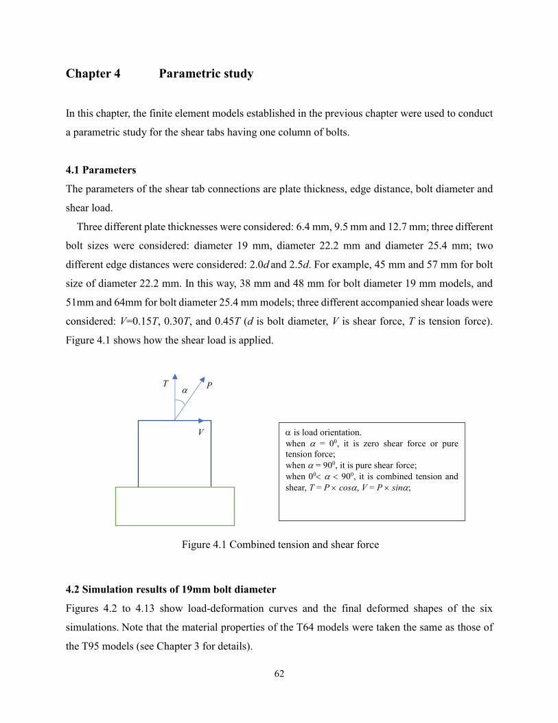
4.1 Parameters
The parameters of the shear tab connections are plate thickness, edge distance, bolt diameter and
shear load.
Three different plate thicknesses were considered: 6.4 mm, 9.5 mm and 12.7 mm; three different
bolt sizes were considered: diameter 19 mm, diameter 22.2 mm and diameter 25.4 mm; two
different edge distances were considered: 2.0d and 2.5d. For example, 45 mm and 57 mm for bolt
size of diameter 22.2 mm. In this way, 38 mm and 48 mm for bolt diameter 19 mm models, and
51mm and 64mm for bolt diameter 25.4 mm models; three different accompanied shear loads were
considered: V=0.15T, 0.30T, and 0.45T (d is bolt diameter, V is shear force, T is tension force).
Figure 4.1 shows how the shear load is applied.
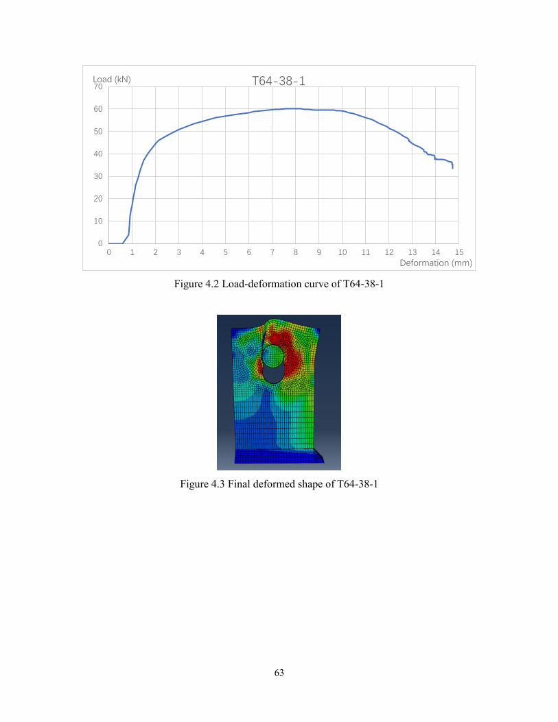
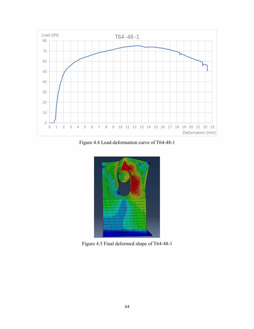
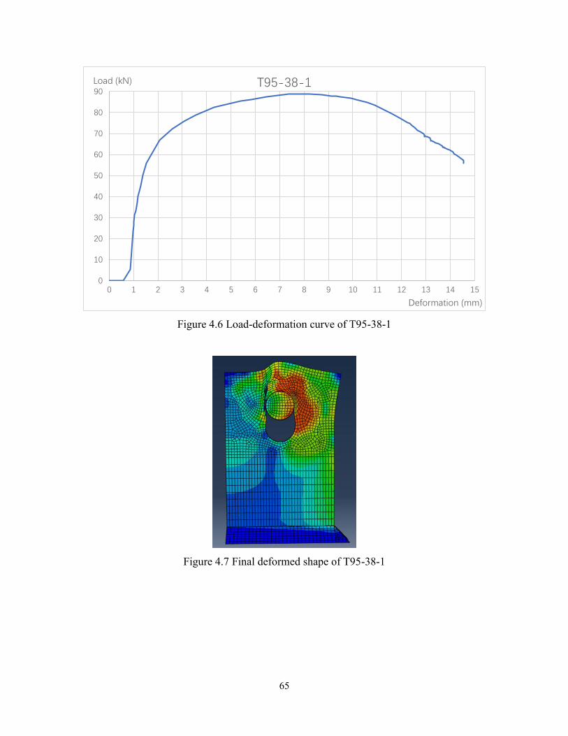
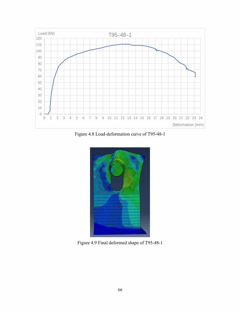
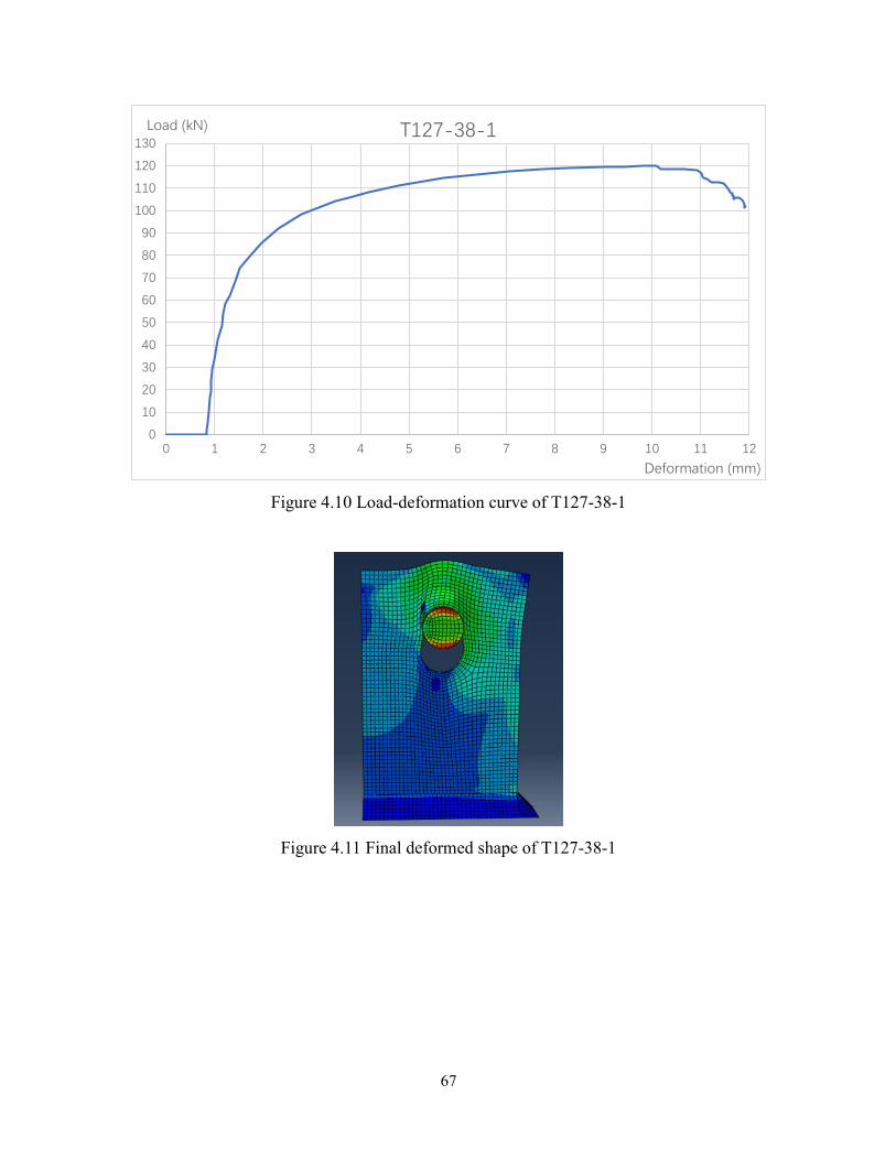
4.2 Simulation results of 19mm bolt diameter
Figures 4.2 to 4.13 show load-deformation curves and the final deformed shapes of the six
simulations. Note that the material properties of the T64 models were taken the same as those of
the T95 models (see Chapter 3 for details).
is load orientation. when = 00, it is zero shear force or pure tension force; when = 900, it is pure shear force; when 00 900, it is combined tension and shear, T = P cos, V = P sin;
Figure 4.1 Combined tension and shear force
T P
V
63
Figure 4.2 Load-deformation curve of T64-38-1
Figure 4.3 Final deformed shape of T64-38-1
0
10
20
30
40
50
60
70
0 1 2 3 4 5 6 7 8 9 10 11 12 13 14 15
Load (kN)
Deformation (mm)
T64-38-1
64
Figure 4.4 Load-deformation curve of T64-48-1
Figure 4.5 Final deformed shape of T64-48-1
0
10
20
30
40
50
60
70
80
0 1 2 3 4 5 6 7 8 9 10 11 12 13 14 15 16 17 18 19 20 21 22 23
Load (kN)
Deformation (mm)
T64-48-1
65
Figure 4.6 Load-deformation curve of T95-38-1
Figure 4.7 Final deformed shape of T95-38-1
0
10
20
30
40
50
60
70
80
90
0 1 2 3 4 5 6 7 8 9 10 11 12 13 14 15
Load (kN)
Deformation (mm)
T95-38-1
66
Figure 4.8 Load-deformation curve of T95-48-1
Figure 4.9 Final deformed shape of T95-48-1
0
10
20
30
40
50
60
70
80
90
100
110
120
0 1 2 3 4 5 6 7 8 9 10 11 12 13 14 15 16 17 18 19 20 21 22 23 24
Load (kN)
Deformation (mm)
T95-48-1
67
Figure 4.10 Load-deformation curve of T127-38-1
Figure 4.11 Final deformed shape of T127-38-1
0
10
20
30
40
50
60
70
80
90
100
110
120
130
0 1 2 3 4 5 6 7 8 9 10 11 12
Load (kN)
Deformation (mm)
T127-38-1
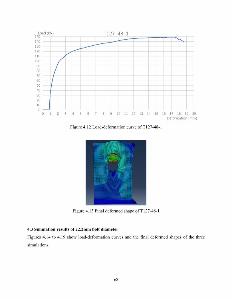
68
Figure 4.12 Load-deformation curve of T127-48-1
Figure 4.13 Final deformed shape of T127-48-1
4.3 Simulation results of 22.2mm bolt diameter
Figures 4.14 to 4.19 show load-deformation curves and the final deformed shapes of the three
simulations.
0
10
20
30
40
50
60
70
80
90
100
110
120
130
140
150
0 1 2 3 4 5 6 7 8 9 10 11 12 13 14 15 16 17 18 19 20
Load (kN)
Deformation (mm)
T127-48-1
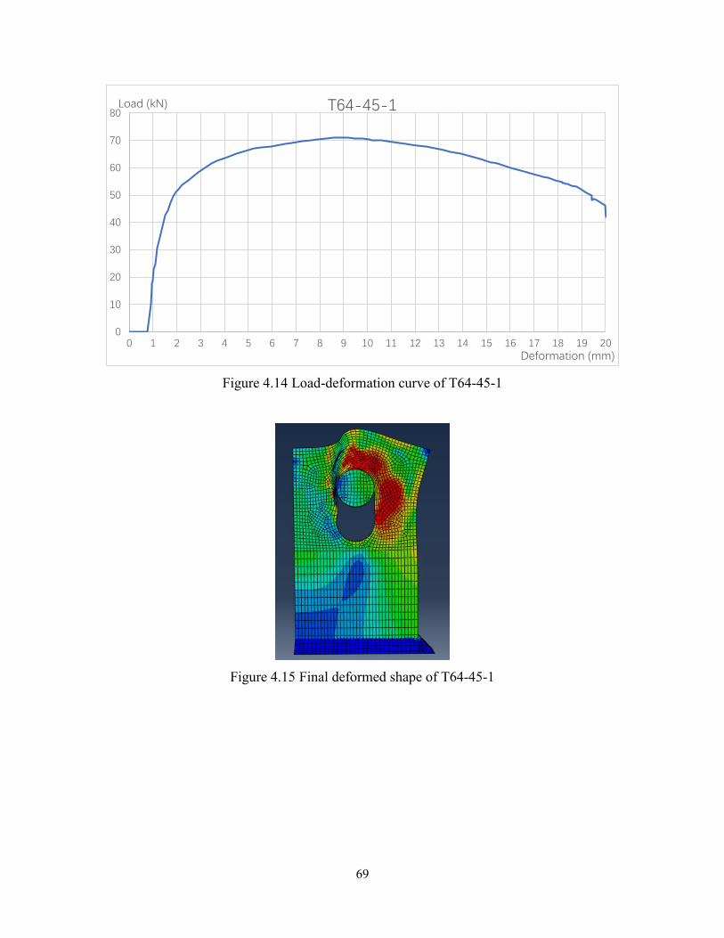
69
Figure 4.14 Load-deformation curve of T64-45-1
Figure 4.15 Final deformed shape of T64-45-1
0
10
20
30
40
50
60
70
80
0 1 2 3 4 5 6 7 8 9 10 11 12 13 14 15 16 17 18 19 20
Load (kN)
Deformation (mm)
T64-45-1
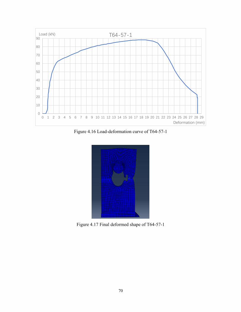
70
Figure 4.16 Load-deformation curve of T64-57-1
Figure 4.17 Final deformed shape of T64-57-1
0
10
20
30
40
50
60
70
80
90
0 1 2 3 4 5 6 7 8 9 10 11 12 13 14 15 16 17 18 19 20 21 22 23 24 25 26 27 28 29
Load (kN)
Deformation (mm)
T64-57-1
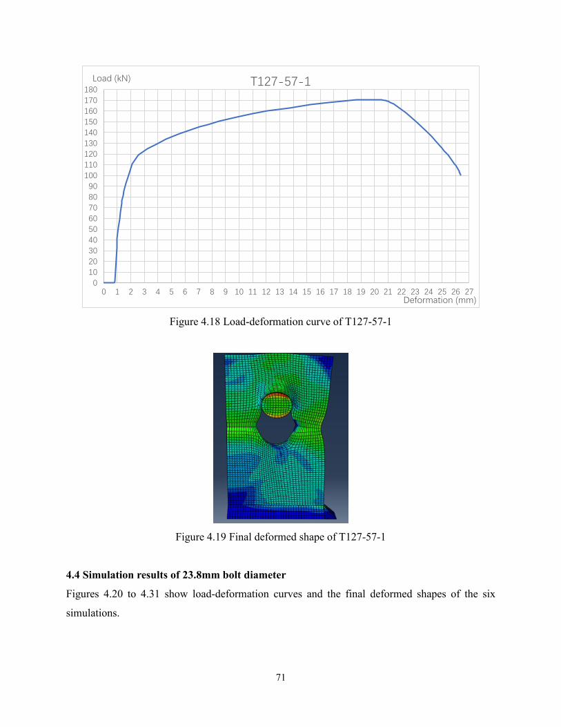
71
Figure 4.18 Load-deformation curve of T127-57-1
Figure 4.19 Final deformed shape of T127-57-1
4.4 Simulation results of 23.8mm bolt diameter
Figures 4.20 to 4.31 show load-deformation curves and the final deformed shapes of the six
simulations.
0102030405060708090
100110120130140150160170180
0 1 2 3 4 5 6 7 8 9 10 11 12 13 14 15 16 17 18 19 20 21 22 23 24 25 26 27
Load (kN)
Deformation (mm)
T127-57-1
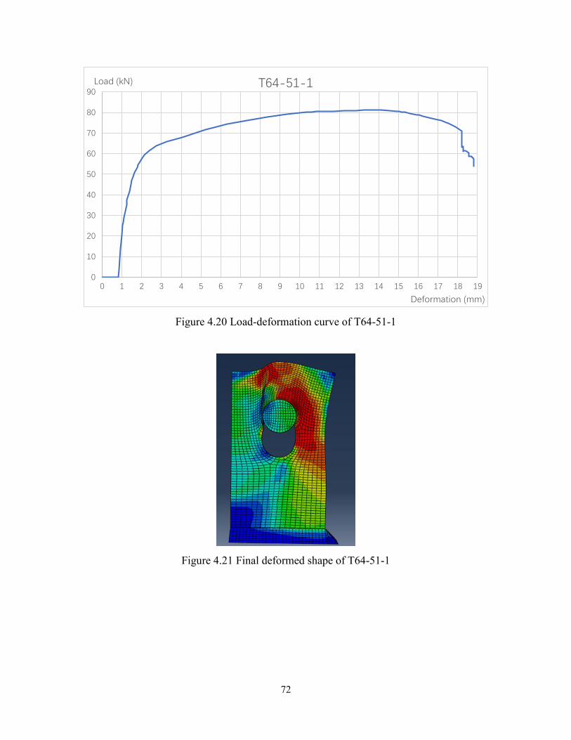
72
Figure 4.20 Load-deformation curve of T64-51-1
Figure 4.21 Final deformed shape of T64-51-1
0
10
20
30
40
50
60
70
80
90
0 1 2 3 4 5 6 7 8 9 10 11 12 13 14 15 16 17 18 19
Load (kN)
Deformation (mm)
T64-51-1
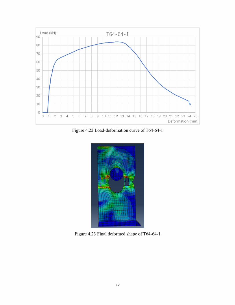
73
Figure 4.22 Load-deformation curve of T64-64-1
Figure 4.23 Final deformed shape of T64-64-1
0
10
20
30
40
50
60
70
80
90
0 1 2 3 4 5 6 7 8 9 10 11 12 13 14 15 16 17 18 19 20 21 22 23 24 25
Load (kN)
Deformation (mm)
T64-64-1
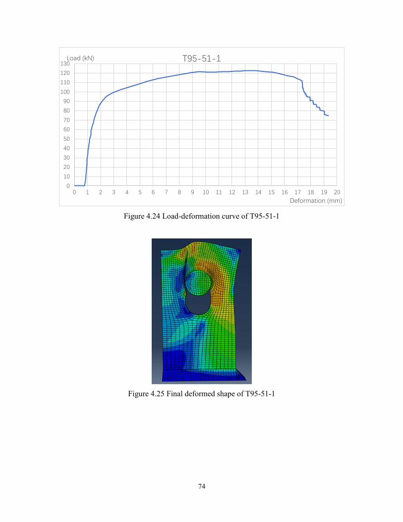
74
Figure 4.24 Load-deformation curve of T95-51-1
Figure 4.25 Final deformed shape of T95-51-1
0
10
20
30
40
50
60
70
80
90
100
110
120
130
0 1 2 3 4 5 6 7 8 9 10 11 12 13 14 15 16 17 18 19 20
Load (kN)
Deformation (mm)
T95-51-1
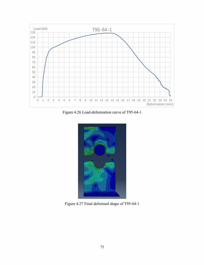
75
Figure 4.26 Load-deformation curve of T95-64-1
Figure 4.27 Final deformed shape of T95-64-1
0
10
20
30
40
50
60
70
80
90
100
110
120
130
0 1 2 3 4 5 6 7 8 9 10 11 12 13 14 15 16 17 18 19 20 21 22 23 24 25
Load (kN)
Deformation (mm)
T95-64-1
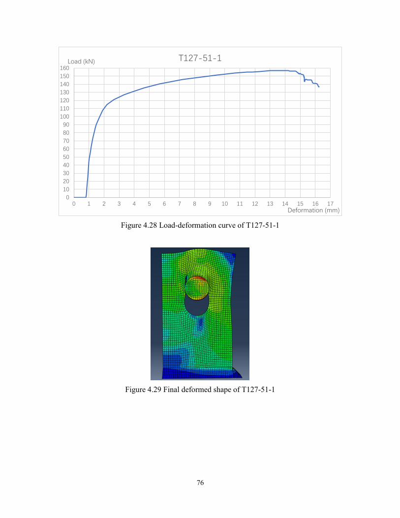
76
Figure 4.28 Load-deformation curve of T127-51-1
Figure 4.29 Final deformed shape of T127-51-1
0
10
20
30
40
50
60
70
80
90
100
110
120
130
140
150
160
0 1 2 3 4 5 6 7 8 9 10 11 12 13 14 15 16 17
Load (kN)
Deformation (mm)
T127-51-1
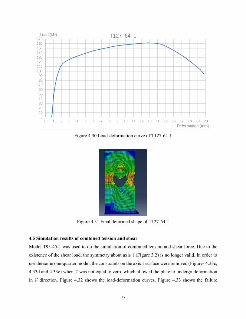
77
Figure 4.30 Load-deformation curve of T127-64-1
Figure 4.31 Final deformed shape of T127-64-1
4.5 Simulation results of combined tension and shear
Model T95-45-1 was used to do the simulation of combined tension and shear force. Due to the
existence of the shear load, the symmetry about axis 1 (Figure 3.2) is no longer valid. In order to
use the same one-quarter model, the constraints on the axis 1 surface were removed (Figures 4.33c,
4.33d and 4.33e) when V was not equal to zero, which allowed the plate to undergo deformation
in V direction. Figure 4.32 shows the load-deformation curves. Figure 4.33 shows the failure
0102030405060708090
100110120130140150160170
0 1 2 3 4 5 6 7 8 9 10 11 12 13 14 15 16 17 18 19 20
Load (kN)
Deformation (mm)
T127-64-1
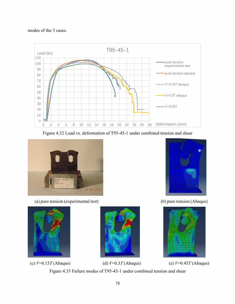
78
modes of the 5 cases.
Figure 4.32 Load vs. deformation of T95-45-1 under combined tension and shear
(a) pure tension (experimental test) (b) pure tension (Abaqus)
(c) V=0.15T (Abaqus) (d) V=0.3T (Abaqus) (e) V=0.45T (Abaqus)
Figure 4.33 Failure modes of T95-45-1 under combined tension and shear
0
10
20
30
40
50
60
70
80
90
100
110
0 2 4 6 8 10 12 14 16 18 20 22 24 26 28
Load (kn)
Deformation (mm)
T95-45-1
pure tensionexperimental test
pure tension abaqus
V=0.15T abaqus
V=0.3T abaqus
V=0.45T
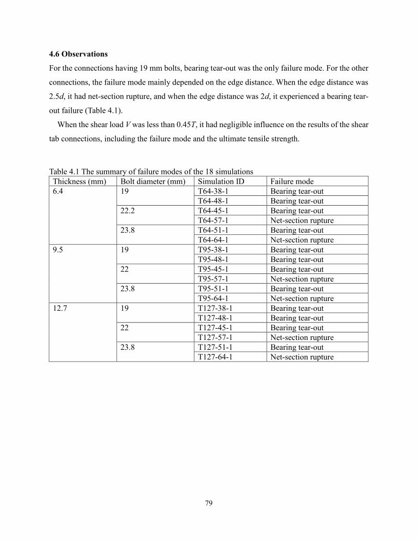
79
4.6 Observations
For the connections having 19 mm bolts, bearing tear-out was the only failure mode. For the other
connections, the failure mode mainly depended on the edge distance. When the edge distance was
2.5d, it had net-section rupture, and when the edge distance was 2d, it experienced a bearing tear-
out failure (Table 4.1).
When the shear load V was less than 0.45T, it had negligible influence on the results of the shear
tab connections, including the failure mode and the ultimate tensile strength.
Table 4.1 The summary of failure modes of the 18 simulations Thickness (mm) Bolt diameter (mm) Simulation ID Failure mode 6.4 19 T64-38-1 Bearing tear-out
T64-48-1 Bearing tear-out 22.2 T64-45-1 Bearing tear-out
T64-57-1 Net-section rupture 23.8 T64-51-1 Bearing tear-out
T64-64-1 Net-section rupture 9.5 19 T95-38-1 Bearing tear-out
T95-48-1 Bearing tear-out 22 T95-45-1 Bearing tear-out
T95-57-1 Net-section rupture 23.8 T95-51-1 Bearing tear-out
T95-64-1 Net-section rupture 12.7 19 T127-38-1 Bearing tear-out
T127-48-1 Bearing tear-out 22 T127-45-1 Bearing tear-out
T127-57-1 Net-section rupture 23.8 T127-51-1 Bearing tear-out
T127-64-1 Net-section rupture
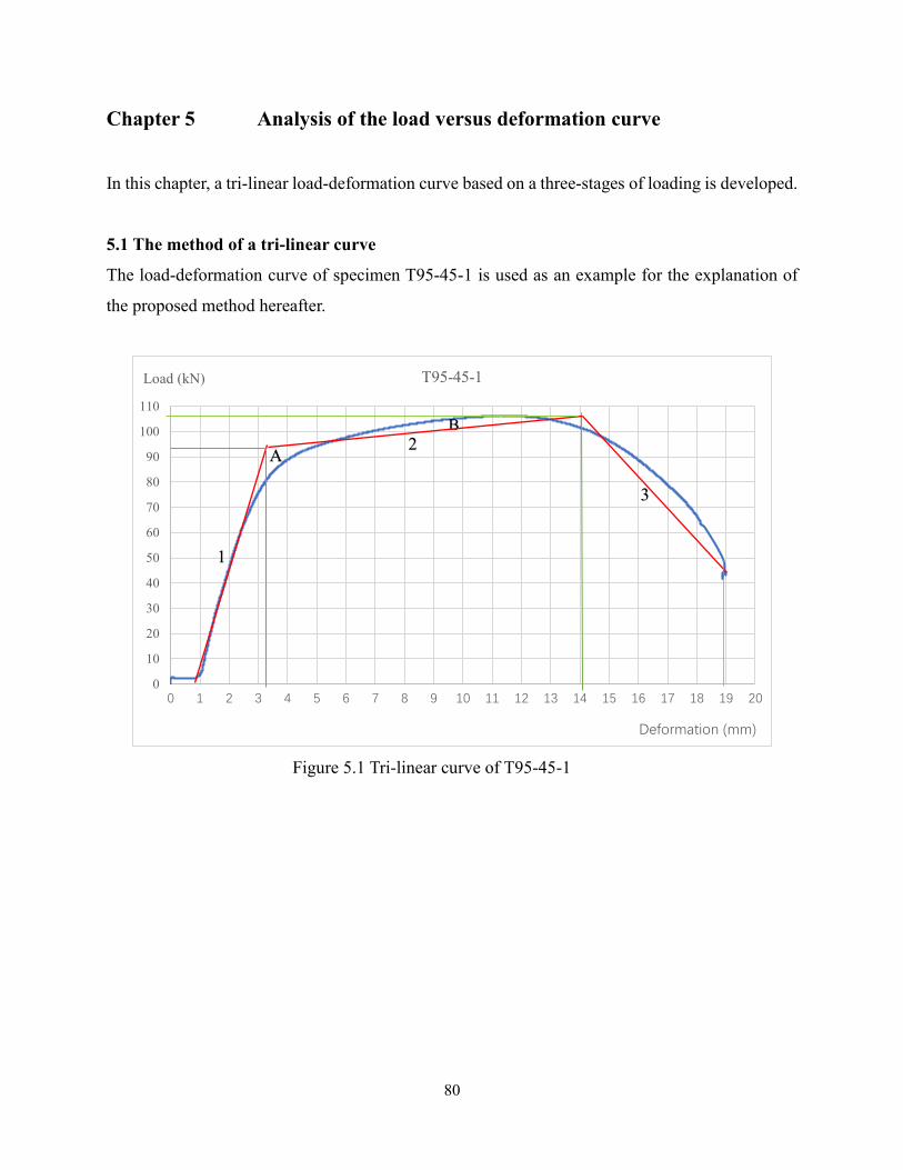
80
Chapter 5 Analysis of the load versus deformation curve
In this chapter, a tri-linear load-deformation curve based on a three-stages of loading is developed.
5.1 The method of a tri-linear curve
The load-deformation curve of specimen T95-45-1 is used as an example for the explanation of
the proposed method hereafter.
Figure 5.1 Tri-linear curve of T95-45-1
0
10
20
30
40
50
60
70
80
90
100
110
0 1 2 3 4 5 6 7 8 9 10 11 12 13 14 15 16 17 18 19 20
Load (kN)
Deformation (mm)
T95-45-1
B2
3
A
1
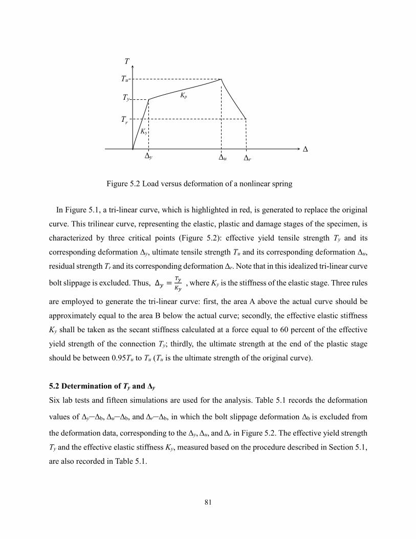
81
In Figure 5.1, a tri-linear curve, which is highlighted in red, is generated to replace the original
curve. This trilinear curve, representing the elastic, plastic and damage stages of the specimen, is
characterized by three critical points (Figure 5.2): effective yield tensile strength Ty and its
corresponding deformation Δy, ultimate tensile strength Tu and its corresponding deformation Δu,
residual strength Tr and its corresponding deformation Δr. Note that in this idealized tri-linear curve
bolt slippage is excluded. Thus, Δ𝑦 =𝑇𝑦
𝐾𝑦 , where Ky is the stiffness of the elastic stage. Three rules
are employed to generate the tri-linear curve: first, the area A above the actual curve should be
approximately equal to the area B below the actual curve; secondly, the effective elastic stiffness
Ky shall be taken as the secant stiffness calculated at a force equal to 60 percent of the effective
yield strength of the connection Ty; thirdly, the ultimate strength at the end of the plastic stage
should be between 0.95Tu to Tu (Tu is the ultimate strength of the original curve).
5.2 Determination of Ty and Δy
Six lab tests and fifteen simulations are used for the analysis. Table 5.1 records the deformation
values of Δy–Δb, Δu–Δb, and Δr–Δb, in which the bolt slippage deformation Δb is excluded from
the deformation data, corresponding to the Δy, Δu, and Δr in Figure 5.2. The effective yield strength
Ty and the effective elastic stiffness Ky, measured based on the procedure described in Section 5.1,
are also recorded in Table 5.1.
Figure 5.2 Load versus deformation of a nonlinear spring
Δ
T
Δr Δy Δu
Tu
Ty
Ky
Kp
Tr
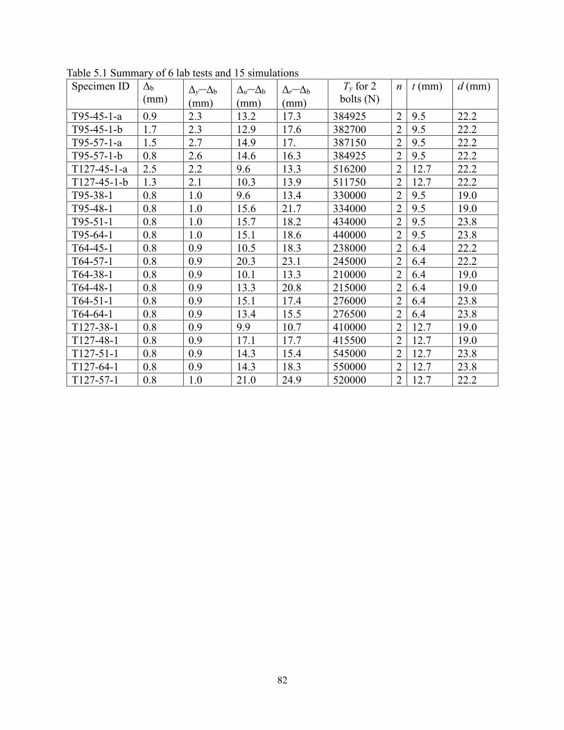
82
Table 5.1 Summary of 6 lab tests and 15 simulations Specimen ID Δb
(mm) Δy–Δb
(mm) Δu–Δb (mm)
Δr–Δb (mm)
Ty for 2 bolts (N)
n t (mm) d (mm)
T95-45-1-a 0.9 2.3 13.2 17.3 384925 2 9.5 22.2 T95-45-1-b 1.7 2.3 12.9 17.6 382700 2 9.5 22.2 T95-57-1-a 1.5 2.7 14.9 17. 387150 2 9.5 22.2 T95-57-1-b 0.8 2.6 14.6 16.3 384925 2 9.5 22.2 T127-45-1-a 2.5 2.2 9.6 13.3 516200 2 12.7 22.2 T127-45-1-b 1.3 2.1 10.3 13.9 511750 2 12.7 22.2 T95-38-1 0.8 1.0 9.6 13.4 330000 2 9.5 19.0 T95-48-1 0.8 1.0 15.6 21.7 334000 2 9.5 19.0 T95-51-1 0.8 1.0 15.7 18.2 434000 2 9.5 23.8 T95-64-1 0.8 1.0 15.1 18.6 440000 2 9.5 23.8 T64-45-1 0.8 0.9 10.5 18.3 238000 2 6.4 22.2 T64-57-1 0.8 0.9 20.3 23.1 245000 2 6.4 22.2 T64-38-1 0.8 0.9 10.1 13.3 210000 2 6.4 19.0 T64-48-1 0.8 0.9 13.3 20.8 215000 2 6.4 19.0 T64-51-1 0.8 0.9 15.1 17.4 276000 2 6.4 23.8 T64-64-1 0.8 0.9 13.4 15.5 276500 2 6.4 23.8 T127-38-1 0.8 0.9 9.9 10.7 410000 2 12.7 19.0 T127-48-1 0.8 0.9 17.1 17.7 415500 2 12.7 19.0 T127-51-1 0.8 0.9 14.3 15.4 545000 2 12.7 23.8 T127-64-1 0.8 0.9 14.3 18.3 550000 2 12.7 23.8 T127-57-1 0.8 1.0 21.0 24.9 520000 2 12.7 22.2
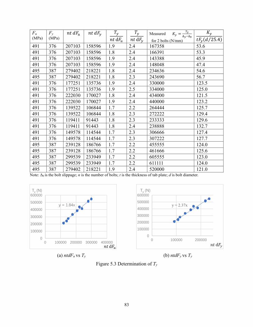
83
Fu (MPa)
Fy (MPa)
𝑛𝑡 ⅆ𝐹𝑢 𝑛𝑡 ⅆ𝐹𝑦 𝑇𝑦
𝑛𝑡 ⅆ𝐹𝑢
𝑇𝑦
𝑛𝑡 ⅆ𝐹𝑦 Measured 𝐾𝑦 =
𝑇𝑦
Δ𝑦−Δ𝑏
for 2 bolts (N/mm) 𝐾𝑦
𝑡𝐹𝑦(ⅆ 25.4⁄ )
491 376 207103 158596 1.9 2.4 167358 53.6 491 376 207103 158596 1.8 2.4 166391 53.3 491 376 207103 158596 1.9 2.4 143388 45.9 491 376 207103 158596 1.9 2.4 148048 47.4 495 387 279402 218221 1.8 2.4 234636 54.6 495 387 279402 218221 1.8 2.3 243690 56.7 491 376 177251 135736 1.9 2.4 330000 123.5 491 376 177251 135736 1.9 2.5 334000 125.0 491 376 222030 170027 1.8 2.4 434000 121.5 491 376 222030 170027 1.9 2.4 440000 123.2 491 376 139522 106844 1.7 2.2 264444 125.7 491 376 139522 106844 1.8 2.3 272222 129.4 491 376 119411 91443 1.8 2.3 233333 129.6 491 376 119411 91443 1.8 2.4 238888 132.7 491 376 149578 114544 1.7 2.3 306666 127.4 491 376 149578 114544 1.7 2.3 307222 127.7 495 387 239128 186766 1.7 2.2 455555 124.0 495 387 239128 186766 1.7 2.2 461666 125.6 495 387 299539 233949 1.7 2.2 605555 123.0 495 387 299539 233949 1.7 2.2 611111 124.0 495 387 279402 218221 1.9 2.4 520000 121.0
Note: Δb is the bolt slippage; n is the number of bolts; t is the thickness of tab plate; d is bolt diameter.
(a) ntdFu vs Ty (b) ntdFy vs Ty
Figure 5.3 Determination of Ty
y = 1.84x
0
100000
200000
300000
400000
500000
600000
0 100000 200000 300000 400000
Ty (N)
𝑛𝑡 ⅆ𝐹𝑢
y = 2.37x
0
100000
200000
300000
400000
500000
600000
0 100000 200000
Ty (N)
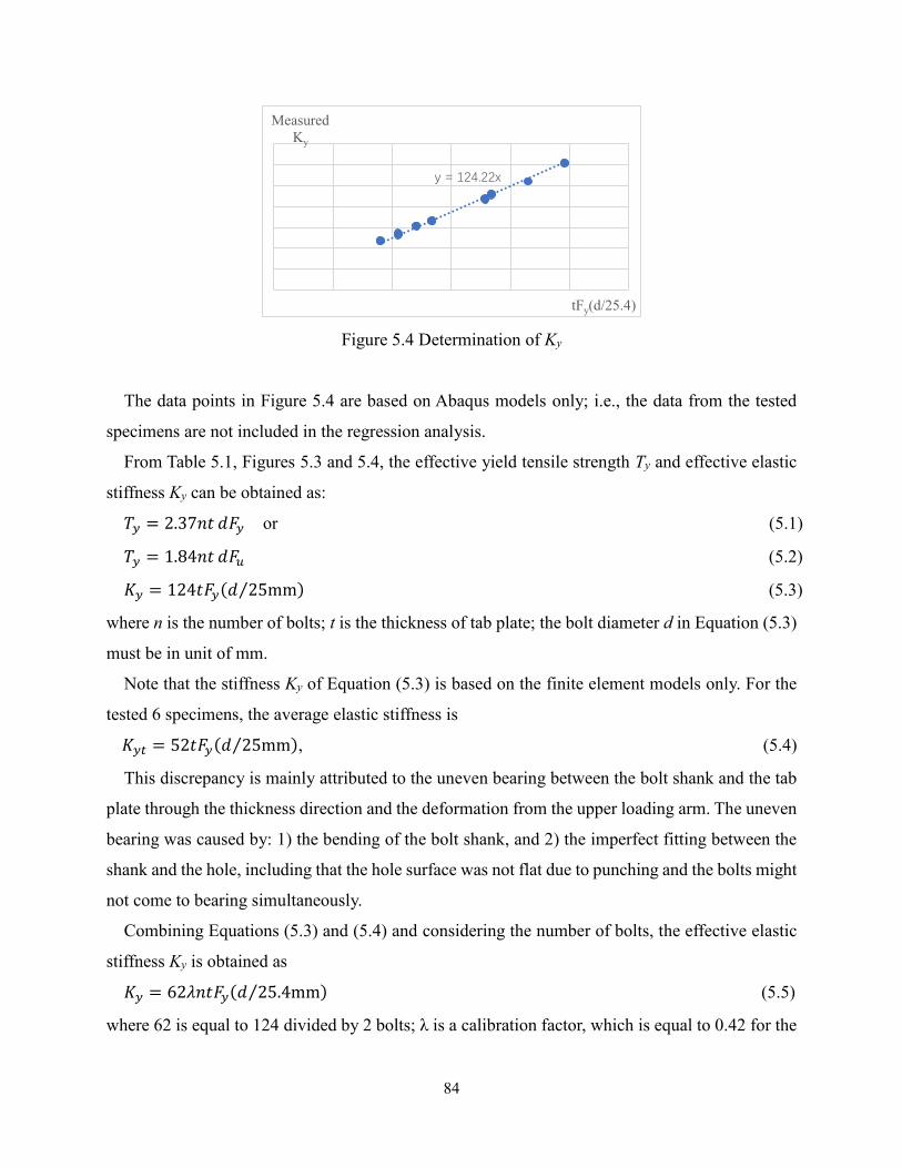
84
Figure 5.4 Determination of Ky
The data points in Figure 5.4 are based on Abaqus models only; i.e., the data from the tested
specimens are not included in the regression analysis.
From Table 5.1, Figures 5.3 and 5.4, the effective yield tensile strength Ty and effective elastic
stiffness Ky can be obtained as:
𝑇𝑦 = 2.37𝑛𝑡 ⅆ𝐹𝑦 or (5.1)
𝑇𝑦 = 1.84𝑛𝑡 ⅆ𝐹𝑢 (5.2)
𝐾𝑦 = 124𝑡𝐹𝑦(ⅆ 25mm⁄ ) (5.3)
where n is the number of bolts; t is the thickness of tab plate; the bolt diameter d in Equation (5.3)
must be in unit of mm.
Note that the stiffness Ky of Equation (5.3) is based on the finite element models only. For the
tested 6 specimens, the average elastic stiffness is
𝐾𝑦𝑡 = 52𝑡𝐹𝑦(ⅆ 25mm⁄ ), (5.4)
This discrepancy is mainly attributed to the uneven bearing between the bolt shank and the tab
plate through the thickness direction and the deformation from the upper loading arm. The uneven
bearing was caused by: 1) the bending of the bolt shank, and 2) the imperfect fitting between the
shank and the hole, including that the hole surface was not flat due to punching and the bolts might
not come to bearing simultaneously.
Combining Equations (5.3) and (5.4) and considering the number of bolts, the effective elastic
stiffness Ky is obtained as
𝐾𝑦 = 62𝜆𝑛𝑡𝐹𝑦(ⅆ 25.4mm⁄ ) (5.5)
where 62 is equal to 124 divided by 2 bolts; λ is a calibration factor, which is equal to 0.42 for the
y = 124.22x
Measured Ky
tFy(d/25.4)
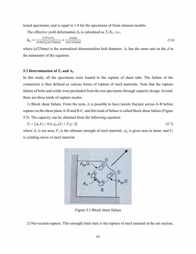
85
tested specimens, and is equal to 1.0 for the specimens of finite element models.
The effective yield deformation Δy is calculated as Ty/Ky, i.e.,
Δ𝑦 =2.37𝑛𝑡 ⅆ𝐹𝑦
62𝜆𝑛𝑡𝐹𝑦(𝑑 25mm⁄ )=
0.038ⅆ
𝜆(𝑑 25mm⁄ ) (5.6)
where (d/25mm) is the normalized dimensionless bolt diameter. Δy has the same unit as the d in
the numerator of the equation.
5.3 Determination of Tu and Δu
In this study, all the specimens were loaded to the rupture of shear tabs. The failure of the
connection is thus defined as various forms of rupture of steel materials. Note that the rupture
failure of bolts and welds were precluded from the test specimens through capacity design. In total,
there are three kinds of rupture modes.
1) Block shear failure. From the tests, it is possible to have tensile fracture across A-B before
rupture on the shear plane A-D and B-C, and this kind of failure is called block shear failure (Figure
5.5). The capacity can be obtained from the following equation:
T1 = [An Fu + 0.6 Agv (Fy + Fu) / 2] (5.7)
where An is net area; Fu is the ultimate strength of steel material; Agv is gross area in shear; and Fy
is yielding stress of steel material.
Figure 5.5 Block shear failure
2) Net-section rupture. This strength limit state is the rupture of steel material at the net section,
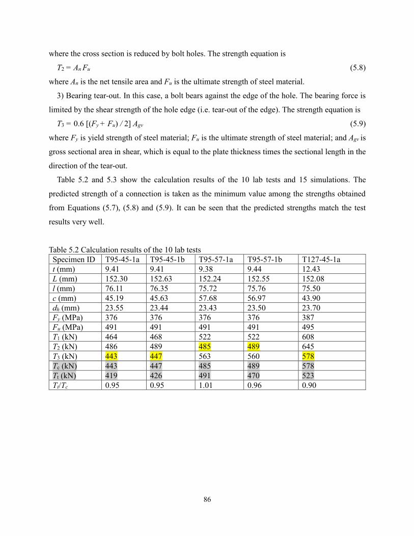
86
where the cross section is reduced by bolt holes. The strength equation is
T2 = An Fu (5.8)
where An is the net tensile area and Fu is the ultimate strength of steel material.
3) Bearing tear-out. In this case, a bolt bears against the edge of the hole. The bearing force is
limited by the shear strength of the hole edge (i.e. tear-out of the edge). The strength equation is
T3 = 0.6 [(Fy + Fu) / 2] Agv (5.9)
where Fy is yield strength of steel material; Fu is the ultimate strength of steel material; and Agv is
gross sectional area in shear, which is equal to the plate thickness times the sectional length in the
direction of the tear-out.
Table 5.2 and 5.3 show the calculation results of the 10 lab tests and 15 simulations. The
predicted strength of a connection is taken as the minimum value among the strengths obtained
from Equations (5.7), (5.8) and (5.9). It can be seen that the predicted strengths match the test
results very well.
Table 5.2 Calculation results of the 10 lab tests Specimen ID T95-45-1a T95-45-1b T95-57-1a T95-57-1b T127-45-1a t (mm) 9.41 9.41 9.38 9.44 12.43 L (mm) 152.30 152.63 152.24 152.55 152.08 l (mm) 76.11 76.35 75.72 75.76 75.50 c (mm) 45.19 45.63 57.68 56.97 43.90 dh (mm) 23.55 23.44 23.43 23.50 23.70 Fy (MPa) 376 376 376 376 387 Fu (MPa) 491 491 491 491 495 T1 (kN) 464 468 522 522 608 T2 (kN) 486 489 485 489 645 T3 (kN) 443 447 563 560 578 Tc (kN) 443 447 485 489 578 Tt (kN) 419 426 491 470 523 Tt/Tc 0.95 0.95 1.01 0.96 0.90
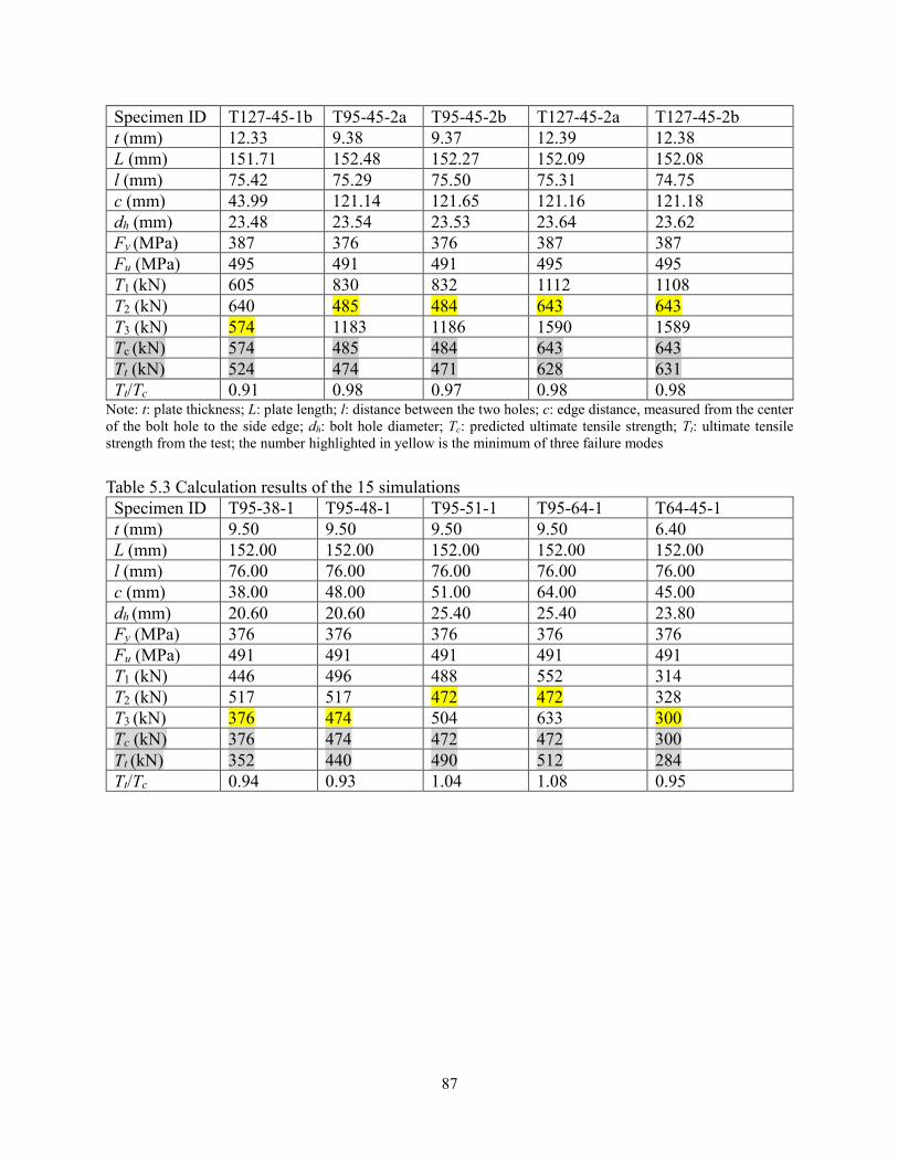
87
Specimen ID T127-45-1b T95-45-2a T95-45-2b T127-45-2a T127-45-2b t (mm) 12.33 9.38 9.37 12.39 12.38 L (mm) 151.71 152.48 152.27 152.09 152.08 l (mm) 75.42 75.29 75.50 75.31 74.75 c (mm) 43.99 121.14 121.65 121.16 121.18 dh (mm) 23.48 23.54 23.53 23.64 23.62 Fy (MPa) 387 376 376 387 387 Fu (MPa) 495 491 491 495 495 T1 (kN) 605 830 832 1112 1108 T2 (kN) 640 485 484 643 643 T3 (kN) 574 1183 1186 1590 1589 Tc (kN) 574 485 484 643 643 Tt (kN) 524 474 471 628 631 Tt/Tc 0.91 0.98 0.97 0.98 0.98
Note: t: plate thickness; L: plate length; l: distance between the two holes; c: edge distance, measured from the center of the bolt hole to the side edge; dh: bolt hole diameter; Tc: predicted ultimate tensile strength; Tt: ultimate tensile strength from the test; the number highlighted in yellow is the minimum of three failure modes
Table 5.3 Calculation results of the 15 simulations Specimen ID T95-38-1 T95-48-1 T95-51-1 T95-64-1 T64-45-1 t (mm) 9.50 9.50 9.50 9.50 6.40 L (mm) 152.00 152.00 152.00 152.00 152.00 l (mm) 76.00 76.00 76.00 76.00 76.00 c (mm) 38.00 48.00 51.00 64.00 45.00 dh (mm) 20.60 20.60 25.40 25.40 23.80 Fy (MPa) 376 376 376 376 376 Fu (MPa) 491 491 491 491 491 T1 (kN) 446 496 488 552 314 T2 (kN) 517 517 472 472 328 T3 (kN) 376 474 504 633 300 Tc (kN) 376 474 472 472 300 Tt (kN) 352 440 490 512 284 Tt/Tc 0.94 0.93 1.04 1.08 0.95

88
Specimen ID T64-57-1 T64-38-1 T64-48-1 T64-51-1 T64-64-1 t (mm) 6.40 6.40 6.40 6.40 6.40 L (mm) 152.00 152.00 152.00 152.00 152.00 l (mm) 76.00 76.00 76.00 76.00 76.00 c (mm) 57.00 38.00 48.00 51.00 64.00 dh (mm) 23.80 20.60 20.60 25.40 25.40 Fy (MPa) 376 376 376 376 376 Fu (MPa) 491 491 491 491 491 T1 (kN) 354 300 334 329 372 T2 (kN) 328 348 348 318 318 T3 (kN) 380 253 320 340 426 Tc (kN) 328 253 320 318 318 Tt (kN) 352 236 300 324 334 Tt/Tc 1.07 0.93 0.94 1.02 1.05
Specimen ID T127-38-1 T127-48-1 T127-51-1 T127-64-1 T127-57-1 t (mm) 12.70 12.70 12.70 12.70 12.70 L (mm) 152.00 152.00 152.00 152.00 152.00 l (mm) 76.00 76.00 76.00 76.00 76.00 c (mm) 38.00 48.00 51.00 64.00 57.00 dh (mm) 20.60 20.60 25.40 25.40 23.80 Fy (MPa) 387 387 387 387 387 Fu (MPa) 495 495 495 495 495 T1 (kN) 604 671 661 748 711 T2 (kN) 697 697 636 636 656 T3 (kN) 511 645 686 860 766 Tc (kN) 511 645 636 636 656 Tt (kN) 480 594 628 636 672 Tt/Tc 0.94 0.92 0.99 1.00 1.02
Note: t: plate thickness; L: plate length; l: distance between the two holes; c: edge distance, measured from the center of the bolt hole to the side edge; dh: bolt hole diameter; Tc: predicted ultimate tensile strength; Tt: ultimate tensile strength from the test; ; the number highlighted in yellow is the minimum of three failure modes
Therefore, the ultimate strength of a connection Tu is obtained as:
Tu = Min { T1, T2, T3 } (5.10)
Whether a connection fails by the rupture of net section or the bearing tear-out is dependent
upon which mode has a smaller tensile capacity. Using Equations (5.8) and (5.9), we can obtain
the following criterion for a net section rupture failure:
An Fu < 0.6 Agv (Fu + Fy )/ 2 (5.11)
where Agv=2ct for one bolt hole, and net area An=t(l – dh) for one bolt. Equation (5.11) is rewritten
as
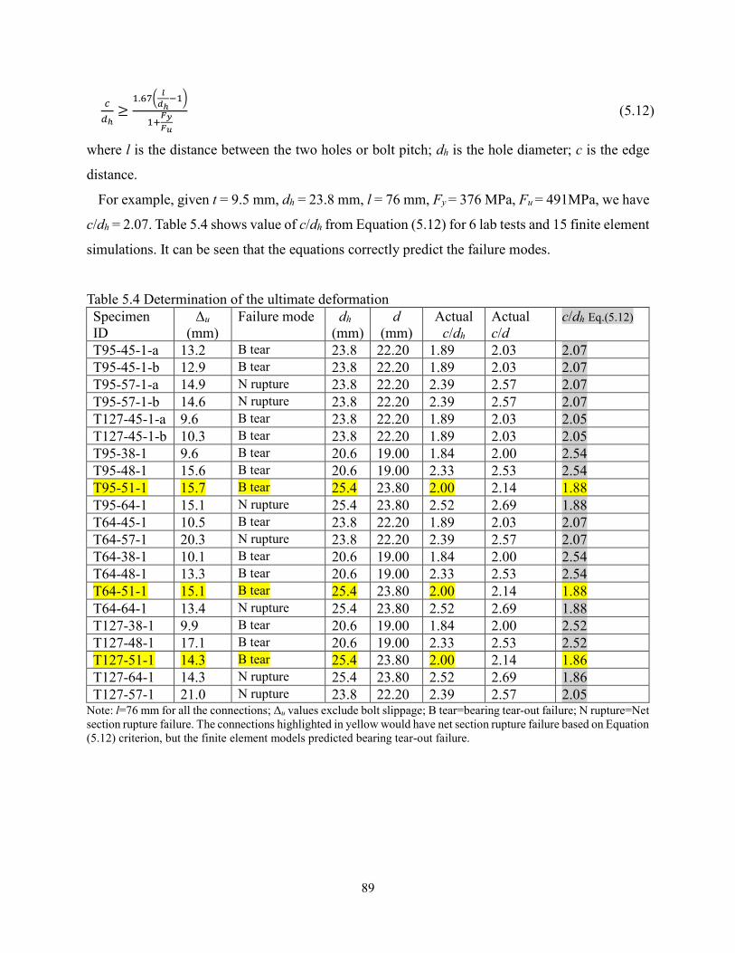
89
𝑐
𝑑ℎ≥
1.67(𝑙
𝑑ℎ−1)
1+𝐹𝑦
𝐹𝑢
(5.12)
where l is the distance between the two holes or bolt pitch; dh is the hole diameter; c is the edge
distance.
For example, given t = 9.5 mm, dh = 23.8 mm, l = 76 mm, Fy = 376 MPa, Fu = 491MPa, we have
c/dh = 2.07. Table 5.4 shows value of c/dh from Equation (5.12) for 6 lab tests and 15 finite element
simulations. It can be seen that the equations correctly predict the failure modes.
Table 5.4 Determination of the ultimate deformation Specimen ID
Δu (mm)
Failure mode dh (mm)
d (mm)
Actual c/dh
Actual c/d
c/dh Eq.(5.12)
T95-45-1-a 13.2 B tear 23.8 22.20 1.89 2.03 2.07 T95-45-1-b 12.9 B tear 23.8 22.20 1.89 2.03 2.07 T95-57-1-a 14.9 N rupture 23.8 22.20 2.39 2.57 2.07 T95-57-1-b 14.6 N rupture 23.8 22.20 2.39 2.57 2.07 T127-45-1-a 9.6 B tear 23.8 22.20 1.89 2.03 2.05 T127-45-1-b 10.3 B tear 23.8 22.20 1.89 2.03 2.05 T95-38-1 9.6 B tear 20.6 19.00 1.84 2.00 2.54 T95-48-1 15.6 B tear 20.6 19.00 2.33 2.53 2.54 T95-51-1 15.7 B tear 25.4 23.80 2.00 2.14 1.88 T95-64-1 15.1 N rupture 25.4 23.80 2.52 2.69 1.88 T64-45-1 10.5 B tear 23.8 22.20 1.89 2.03 2.07 T64-57-1 20.3 N rupture 23.8 22.20 2.39 2.57 2.07 T64-38-1 10.1 B tear 20.6 19.00 1.84 2.00 2.54 T64-48-1 13.3 B tear 20.6 19.00 2.33 2.53 2.54 T64-51-1 15.1 B tear 25.4 23.80 2.00 2.14 1.88 T64-64-1 13.4 N rupture 25.4 23.80 2.52 2.69 1.88 T127-38-1 9.9 B tear 20.6 19.00 1.84 2.00 2.52 T127-48-1 17.1 B tear 20.6 19.00 2.33 2.53 2.52 T127-51-1 14.3 B tear 25.4 23.80 2.00 2.14 1.86 T127-64-1 14.3 N rupture 25.4 23.80 2.52 2.69 1.86 T127-57-1 21.0 N rupture 23.8 22.20 2.39 2.57 2.05
Note: l=76 mm for all the connections; Δu values exclude bolt slippage; B tear=bearing tear-out failure; N rupture=Net section rupture failure. The connections highlighted in yellow would have net section rupture failure based on Equation (5.12) criterion, but the finite element models predicted bearing tear-out failure.
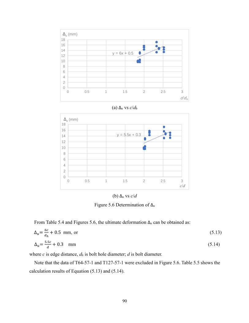
90
(a) ∆u vs c/dh
(b) ∆u vs c/d
Figure 5.6 Determination of ∆u
From Table 5.4 and Figures 5.6, the ultimate deformation ∆u can be obtained as:
∆𝑢=6𝑐
𝑑ℎ+ 0.5 mm, or (5.13)
∆𝑢=5.5𝑐
𝑑+ 0.3 mm (5.14)
where c is edge distance, dh is bolt hole diameter; d is bolt diameter.
Note that the data of T64-57-1 and T127-57-1 were excluded in Figure 5.6. Table 5.5 shows the
calculation results of Equation (5.13) and (5.14).
y = 6x + 0.5
0
2
4
6
8
10
12
14
16
18
0 0.5 1 1.5 2 2.5 3
∆u (mm)
c/dh
y = 5.5x + 0.3
0
2
4
6
8
10
12
14
16
18
0 0.5 1 1.5 2 2.5 3
∆u (mm)
c/d
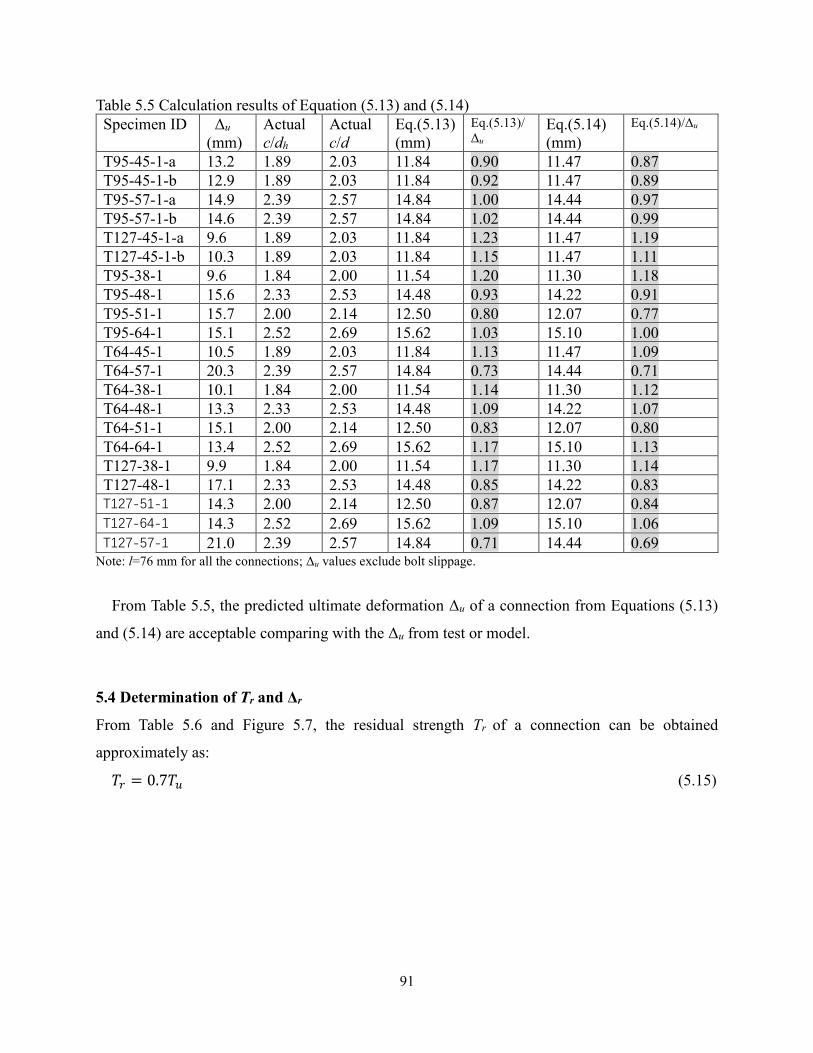
91
Table 5.5 Calculation results of Equation (5.13) and (5.14) Specimen ID Δu
(mm) Actual c/dh
Actual c/d
Eq.(5.13) (mm)
Eq.(5.13)/Δu
Eq.(5.14) (mm)
Eq.(5.14)/Δu
T95-45-1-a 13.2 1.89 2.03 11.84 0.90 11.47 0.87 T95-45-1-b 12.9 1.89 2.03 11.84 0.92 11.47 0.89 T95-57-1-a 14.9 2.39 2.57 14.84 1.00 14.44 0.97 T95-57-1-b 14.6 2.39 2.57 14.84 1.02 14.44 0.99 T127-45-1-a 9.6 1.89 2.03 11.84 1.23 11.47 1.19 T127-45-1-b 10.3 1.89 2.03 11.84 1.15 11.47 1.11 T95-38-1 9.6 1.84 2.00 11.54 1.20 11.30 1.18 T95-48-1 15.6 2.33 2.53 14.48 0.93 14.22 0.91 T95-51-1 15.7 2.00 2.14 12.50 0.80 12.07 0.77 T95-64-1 15.1 2.52 2.69 15.62 1.03 15.10 1.00 T64-45-1 10.5 1.89 2.03 11.84 1.13 11.47 1.09 T64-57-1 20.3 2.39 2.57 14.84 0.73 14.44 0.71 T64-38-1 10.1 1.84 2.00 11.54 1.14 11.30 1.12 T64-48-1 13.3 2.33 2.53 14.48 1.09 14.22 1.07 T64-51-1 15.1 2.00 2.14 12.50 0.83 12.07 0.80 T64-64-1 13.4 2.52 2.69 15.62 1.17 15.10 1.13 T127-38-1 9.9 1.84 2.00 11.54 1.17 11.30 1.14 T127-48-1 17.1 2.33 2.53 14.48 0.85 14.22 0.83 T127-51-1 14.3 2.00 2.14 12.50 0.87 12.07 0.84 T127-64-1 14.3 2.52 2.69 15.62 1.09 15.10 1.06 T127-57-1 21.0 2.39 2.57 14.84 0.71 14.44 0.69
Note: l=76 mm for all the connections; Δu values exclude bolt slippage.
From Table 5.5, the predicted ultimate deformation Δu of a connection from Equations (5.13)
and (5.14) are acceptable comparing with the Δu from test or model.
5.4 Determination of Tr and Δr
From Table 5.6 and Figure 5.7, the residual strength Tr of a connection can be obtained
approximately as:
𝑇𝑟 = 0.7𝑇𝑢 (5.15)
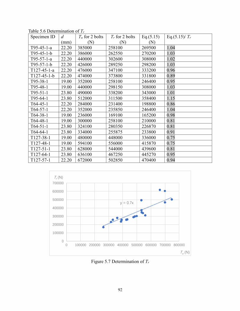
92
Table 5.6 Determination of Tr Specimen ID d
(mm) Tu for 2 bolts
(N) Tr for 2 bolts
(N) Eq.(5.15)
(N) Eq.(5.15)/ Tr
T95-45-1-a 22.20 385000 258100 269500 1.04 T95-45-1-b 22.20 386000 262550 270200 1.03 T95-57-1-a 22.20 440000 302600 308000 1.02 T95-57-1-b 22.20 426000 289250 298200 1.03 T127-45-1-a 22.20 476000 347100 333200 0.96 T127-45-1-b 22.20 474000 373800 331800 0.89 T95-38-1 19.00 352000 258100 246400 0.95 T95-48-1 19.00 440000 298150 308000 1.03 T95-51-1 23.80 490000 338200 343000 1.01 T95-64-1 23.80 512000 311500 358400 1.15 T64-45-1 22.20 284000 231400 198800 0.86 T64-57-1 22.20 352000 235850 246400 1.04 T64-38-1 19.00 236000 169100 165200 0.98 T64-48-1 19.00 300000 258100 210000 0.81 T64-51-1 23.80 324100 280350 226870 0.81 T64-64-1 23.80 334000 255875 233800 0.91 T127-38-1 19.00 480000 448000 336000 0.75 T127-48-1 19.00 594100 556000 415870 0.75 T127-51-1 23.80 628000 544000 439600 0.81 T127-64-1 23.80 636100 467250 445270 0.95 T127-57-1 22.20 672000 502850 470400 0.94
Figure 5.7 Determination of Tr
y = 0.7x
0
100000
200000
300000
400000
500000
600000
700000
0 100000 200000 300000 400000 500000 600000 700000 800000
Tr (N)
Tu (N)
93
Table 5.7 Determination of Δr
Specimen ID Δr (mm)
Actual c/dh
Actual c/d
Eq.(5.16) (mm)
Eq.(5.16)/Δr
Eq.(5.17) (mm)
Eq.(5.17)/Δr
T95-45-1-a 17.3 1.89 2.03 16.01 0.93 15.73 0.91 T95-45-1-b 17.6 1.89 2.03 16.01 0.91 15.73 0.89 T95-57-1-a 17.0 2.39 2.57 18.26 1.07 18.05 1.06 T95-57-1-b 16.3 2.39 2.57 18.26 1.12 18.05 1.11 T127-45-1-a 13.3 1.89 2.03 16.01 1.20 15.73 1.18 T127-45-1-b 13.9 1.89 2.03 16.01 1.15 15.73 1.13 T95-38-1 13.4 1.84 2.00 15.78 1.18 15.60 1.16 T95-48-1 21.7 2.33 2.53 17.99 0.83 17.88 0.82 T95-51-1 18.2 2.00 2.14 16.50 0.91 16.20 0.89 T95-64-1 18.6 2.52 2.69 18.84 1.01 18.57 1.00 T64-45-1 18.3 1.89 2.03 16.01 0.87 15.73 0.86 T64-57-1 23.1 2.39 2.57 18.26 0.79 18.05 0.78 T64-38-1 13.3 1.84 2.00 15.78 1.19 15.60 1.17 T64-48-1 20.8 2.33 2.53 17.99 0.86 17.88 0.86 T64-51-1 17.4 2.00 2.14 16.50 0.95 16.20 0.93 T64-64-1 15.5 2.52 2.69 18.84 1.22 18.57 1.20 T127-38-1 10.7 1.84 2.00 15.78 1.47 15.60 1.46 T127-48-1 17.7 2.33 2.53 17.99 1.02 17.88 1.01 T127-51-1 15.4 2.00 2.14 16.50 1.07 16.20 1.05 T127-64-1 18.3 2.52 2.69 18.84 1.03 18.57 1.01 T127-57-1 24.9 2.39 2.57 18.26 0.73 18.05 0.72
Note: l=76 mm for all the connections; Δr values exclude bolt slippage.
(a) ∆r vs. c/dh
y = 4.5x + 7.5
0
5
10
15
20
25
0 0.5 1 1.5 2 2.5 3
∆r (mm)
c/dh
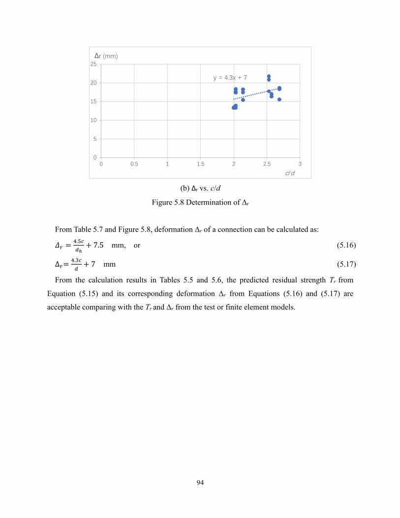
94
(b) ∆r vs. c/d
Figure 5.8 Determination of Δr
From Table 5.7 and Figure 5.8, deformation Δr of a connection can be calculated as:
𝛥𝑟 =4.5𝑐
𝑑ℎ+ 7.5 mm, or (5.16)
∆𝑟=4.3𝑐
𝑑+ 7 mm (5.17)
From the calculation results in Tables 5.5 and 5.6, the predicted residual strength Tr from
Equation (5.15) and its corresponding deformation Δr from Equations (5.16) and (5.17) are
acceptable comparing with the Tr and Δr from the test or finite element models.
y = 4.3x + 7
0
5
10
15
20
25
0 0.5 1 1.5 2 2.5 3
∆r (mm)
c/d
95
Chapter 6 Conclusions and future works
This chapter summarizes the research work of this thesis and provides some recommendations for
future studies.
6.1 Summary and conclusions
This thesis consists of four parts: lab test, finite element modeling, parametric study, and load-
deformation curve.
First, the test of two series of coupons and ten shear tab connections under a pure tension load
were performed. The coupon test results included the material properties such as yield strength,
ultimate strength and necking initiation strain. The shear tab connection test results included the
failure modes and the load-deformation curves.
Second, software Abaqus was used to simulate the pure tension test of the shear tab connections.
The test load-deformation curves and failure modes were used to calibrate the finite element
models.
Third, the verified finite element models were employed to conduct a parametric study. Four
parameters, i.e., plate thickness, edge distance, bolt diameter and shear load, were studied, which
resulted in 15 simulations.
Last, a tri-linear curve was developed to predict the load versus deformation relationship of a
shear tab connection having one-column bolts.
The following conclusions can be drawn from this research work:
1) Tensile rupture of the net section and bearing tear-out of the bolt hole side edge were the
typical failure modes of the tested shear tab connections, for which the rupture of bolts or welds
was precluded by a capacity design principle.
2) All the connections exhibited good ductility, i.e., experienced large plastic deformation before
a rupture failure.
3) When the accompanying shear load was less than 45 percent of the tensile load, the impact
of the shear load on the tensile strength and the tensile deformation of the shear tab connections
could be ignored.
4) The actual load-deformation curves of the shear tab connections could be represented by a
tri-linear curve, whose values at the three critical points are given by Equations (5.1) and (5.6),
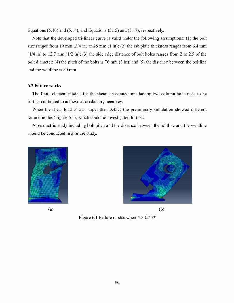
96
Equations (5.10) and (5.14), and Equations (5.15) and (5.17), respectively.
Note that the developed tri-linear curve is valid under the following assumptions: (1) the bolt
size ranges from 19 mm (3/4 in) to 25 mm (1 in); (2) the tab plate thickness ranges from 6.4 mm
(1/4 in) to 12.7 mm (1/2 in); (3) the side edge distance of bolt holes ranges from 2 to 2.5 of the
bolt diameter; (4) the pitch of the bolts is 76 mm (3 in); and (5) the distance between the boltline
and the weldline is 80 mm.
6.2 Future works
The finite element models for the shear tab connections having two-column bolts need to be
further calibrated to achieve a satisfactory accuracy.
When the shear load V was larger than 0.45T, the preliminary simulation showed different
failure modes (Figure 6.1), which could be investigated further.
A parametric study including bolt pitch and the distance between the boltline and the weldline
should be conducted in a future study.
(a) (b)
Figure 6.1 Failure modes when V 0.45T
97
References Arasaratnam, P., Sivakumaran, K. S., & Tait, M. J. (2011). True stress-true strain models for
structural steel elements. ISRN Civil Engineering, 2011, 1-11.
Ashakul, A. (2004). Finite Element Analysis of Single Plate Shear Connections (Doctoral
dissertation, Virginia Tech).
Astaneh-Asl, A., McMullin, K.M., & Call, S. M. (1993). Behavior and design of steel single plate
shear connections. Journal of Structural Engineering, 119(8), 2421-2440.
Canadian Institute of Steel Construction. (2014). CAS/S16-14 Design of steel structure.
Canadian Standards Association, Toronto, ON, Canada.
Daneshvar H. & Driver R. G. (2011). Behavior of shear tab connections under column removal
scenario. In Structures Congress 2011 (pp. 2905 -2916).
Daneshvar, H., & Driver, R. G. (2017). Behaviour of shear tab connections in column removal
scenario. Journal of Constructional Steel Research, 138, 580-593.
Ehlers, S., & Varsta, P. (2009). Strain and stress relation for non-linear finite element simulations.
Thin-Walled Structures, 47(11), 1203-1217.
Ferrell, M. T. (2003). Designing with single plate connections. Modern Steel Construction, 43(4),
51-53.
Gong, Y. (2009). Design moment of shear connections at the ultimate limit state. Journal of
Constructional Steel Research, 65(10-11), 1921-1930.
Gong, Y. (2010). Analysis and design for the resilience of shear connections. Canadian Journal of
Civil Engineering, 37(12), 1581-1589.
Gong, Y. (2014). Ultimate tensile deformation and strength capacities of bolted-angle connections.
Journal of Constructional Steel Research, 100, 50-59.
Gong, Y. (2017). Test, modeling and design of bolted-angle connections subjects to column
removal. Journal of Constructional Steel Research, 139, 315-326.
Guravich, S. J., & Dawe, J. L. (2006). Simple beam connections in combined shear and tension,
Canadian Journal of Civil Engineering, 33(4), 357-372.
Hibbeler, R. C. (2014). Mechanics of Materials. US: Pearson Prentice Hall.
Hibbitt, K & Sorensen, I. (2000). ABAQUS/CAE User’s Manual. US: Boston.
Kiran, R., & Khandelwal, K. (2014). A triaxiality and Lode parameter dependent ductile fracture
criterion. Engineering Fracture Mechanics, 128, 121-138.
98
Levanger, H. (2012). Simulating Ductile Fracture in Steel Using the Finite Element Mothed:
Comparison of Two Models for Describing Local Instability due to Ductile Fracture (Master’s
thesis).
Lipson, S. L. (1968, February). Single-angle and single-plate beam framing connections. In
Canadian Structural Engineering Conference, Toronto, Ontario (pp. 141-162).
Logan, D. L. (2006). A First Course in the Finite Element Method. US: Chris Carson.
Mirzaei, A. (2014). Steel Shear Tab Connections Subjected to Combined Shear and Axial Forces
(Doctoral dissertation: McGill University).
Oosterhof, S. A. & Driver, R. G. (2011). Performance of Steel Shear Connections under Combined
Moment, Shear, and Tension. Journal of Structural Engineering, ASCE, University of Alberta,
AB.
Oosterhof, S. A., & Driver, R. G. (2014). Behavior of steel shear connections under column-
removal demands. Journal of Structural Engineering, ASCE, 141(4), 04014126.
Oosterhof, S. A., & Driver, R. G. (2016). Shear connection modelling for column removal analysis.
Journal of Constructional Steel Research, 117, 227-242.
Rex, C. O., & Easterling, W. S. (1996). Behavior and modeling of partially restrained composite
beam-girder connections (Virginia Polytechnic Institute and State University).
Rex, C. O., & Eastering, W. S. (2003). Behavior and modeling of a bolt bearing on a single plate.
Journal of Structural Engineering, 129(6), 792-800.
Roddis, W. K., & Blass, D. (2013). Tensile capacity of single-angle shear connections considering
prying action. Journal of Structural Engineering, 139(4), 504-514.
Sancho, A., Cox, M. J., Cartwright, T., Aldrich-Smith, G. D., Hooper, P. A., Davies, C. M., & Dear,
J. P. (2016). Experimental techniques for ductile damage characterization. Procedia Structural
Integrity, 2, 966-973.
Thompson, S. L. (2009). Axial, Shear and Moment Interaction of Single Plate “Shear Tab”
Connections (Doctoral dissertation, Milwaukee School of Engineering).
Torrentallé Dot, M. (2015). High strength steel fracture: fracture initiation analysis by the essential
work of fracture concept (Bachelor's thesis, Universitat Politècnica de Catalunya).
Yang, B., & Tan, K. H. (2013). Robustness of bolted-angle connections against progressive
collapse: Experimental tests of beam-column joints and development of component-based
models. Journal of Structural Engineering, ASCE, 139(9), 1498-1514.