2017 Quantizations of the torus -...

BEREZIN-TOEPLITZ QUANTIZATION AND COMPLEX WEYL

QUANTIZATION OF THE TORUS T2.

OPHÉLIE ROUBY

Abstract. In this paper, we give a correspondence between the Berezin-Toeplitz and the complex Weyl quantizations of the torus T2. To achieve this,we use the correspondence between the Berezin-Toeplitz and the complex Weylquantizations of the complex plane and a relation between the Berezin-Toeplitzquantization of a periodic symbol on the real phase space R2 and the Berezin-Toeplitz quantization of a symbol on the torus T2.

Introduction

The object of this paper is to construct a new semi-classical quantization of thetorus T2 by adapting Sjöstrand’s complex Weyl quantization of R2 and to givethe correspondence between this quantization and the well-known Berezin-Toeplitzquantization of T2. When the phase space is R2n, the pseudo-differential Weylquantization allows us to relate a classical system to a quantum one through thesymbol map; thus pseudo-differential operators have become an important tool inquantum mechanics. On the mathematical side, these operators have been intro-duced in the mid-sixties by André Unterberger and Juliane Bokobza [UB64] and inparallel by Joseph Kohn and Louis Nirenberg [KN65] and have been investigated byLars Hörmander [Hör65, Hör66, Hör67]. They allow to study physical systems inpositions and momenta. On the other hand, Berezin-Toeplitz operators have beenintroduced by Feliks Berezin [Ber75] and investigated by Louis Boutet de Mon-vel and Victor Guillemin [BdMG81] as a generalization of Toeplitz matrices. Thestudy of these operators has been motivated by the fact that pseudo-differentialoperators take into account only phases spaces that can be written as cotangentspaces, whereas in mechanics, there are physical observables like spin that naturallylives on other types of phases spaces, like compact Kähler manifolds, which can bequantized in the Berezin-Toeplitz way. In fact, it was realized recently that theBerezin-Toeplitz quantization applies to even more general symplectic manifolds,and thus has become a tool of choice for applications of symplectic geometry andtopology, see [CP16].

In this paper, we give a relation between the Berezin-Toeplitz quantization of thetorus, studied for instance by David Borthwick and Alejandro Uribe in [BU03] andthe complex Weyl quantization of the torus, which we introduce as a variation ofSjöstrand’s quantization of R2. The complex Weyl quantization of R2 has beeninvestigated by Johannes Sjöstrand in [Sjö02], then by Anders Melin and JohannesSjöstrand in [MS02, MS03], also by Michael Hitrik and Johannes Sjöstrand in [HS04]and in their mini-courses [HS15] and by Michael Hitrik, Johannes Sjöstrand and San

1

2 OPHÉLIE ROUBY

Vu Ngo.c in [HSN07]. This quantization of the real plane R2 allows to study pseudo-differential operators with complex symbols, and therefore is particularly useful forproblems involving non self-adjoint operators or quantum resonances. It is definedby a contour integral over an IR-manifold (I-Lagrangian and R-symplectic) whichplays the role of the phase space. Here, we define an analogue of this notion in thetorus case.If we consider the complex plane as a phase space, there exists a correspondencebetween the complex Weyl and the Berezin-Toeplitz quantizations (this correspon-dence uses a variant of Bargmann’s transform and can be found, for instance, inthe book [Zwo12, chapter 13] of Maciej Zworski); using this result, we are able toobtain Bohr-Sommerfeld quantization conditions for non-selfadjoint perturbationsof self-adjoint Berezin-Toeplitz operators of the complex plane C by first provingthe result in the case of pseudo-differential operators (see [Rou17]). Therefore, weexpect that this new complex quantization of T2, together with its relationship tothe Berezin-Toeplitz quantization, will be crucial in obtaining precise eigenvalueasymptotics of non-selfadjoint Berezin-Toeplitz operators on the torus.

Structure of the paper:

• in Section 1, we state our result;• in Section 2, we give the proof of our result which is divided into three

parts, the first one consists in recalling the Berezin-Toeplitz quantizationof the torus, the second one in introducing the complex Weyl quantizationof the torus and the last one in relating these two quantizations.

Acknowledgements. The author would like to thank both San Vu Ngo.c andLaurent Charles for their support and guidance. Funding was provided by theUniversité de Rennes 1 and the Centre Henri Lebesgue.

1. Result

1.1. Context. In this section, we recall the definition of the Berezin-Toeplitz quan-tization of a symbol on the torus T2 (see for example [CM15]) and we give a defi-nition of the complex Weyl quantization of a symbol on the torus. Let 0 < ~ ≤ 1be the semi-classical parameter. By convention the Weyl quantization involves thesemi-classical parameter ~, contrary to the Berezin-Toeplitz quantization which in-volves the inverse of this parameter, denoted by k. In the whole paper, we will usethese two parameters.

Notation: let k be an integer greater than 1. Let u and v be complex numbers ofmodulus 1.

• If z ∈ C, we denote by z = (p, q) ∈ R2 or z = p+ iq via the identificationof C with R2.

• T2 denotes the torus (R/2πZ)× (R/Z).

• Gk is the space of measurable functions g such that:

∫ 2π

0

∫ 1

0

|g(p, q)|2 e−kq2dpdq < +∞,

QUANTIZATIONS OF THE TORUS 3

which are invariant under the action of the Heisenberg group (for moredetails, see Subsection 2.1), i.e. for all (p, q) ∈ R2, we have:

g(p+ 2π, q) = ukg(p, q) and g(p, q + 1) = vke−i(p+iq)k+k/2g(p, q).

• Hk is the space of holomorphic functions in Gk, i.e.:

Hk ={

g ∈ Hol(C); g(p+ 2π, q) = ukg(p, q), g(p, q + 1) = vke−i(p+iq)k+k/2g(p, q)}

.

• Πk is the orthogonal projection of the space Gk (equipped with the weightedL2-scalar product on [0, 2π]× [0, 1]) on the space Hk.

Remark 1.1.1.

• The spaces Gk and Hk depend on the complex numbers u and v.• In [BU03], they consider the torus T2 = R2/Z2 and they choose an other

quantization which leads to an other space of holomorphic functions, alsocalled Hk, defined as follows:

Hk ={

g ∈ Hol(C); ∀(m,n) ∈ Z2, g(z +m+ in) = (−1)kmnekπ(z(m−in)+(1/2)(m2+n2))g(z)

}

.

Definition 1.1.2 (Asymptotic expansion). Let fk ∈ C∞(R2). We say that fk ad-mits an asymptotic expansion in powers of 1/k for the C∞-topology of the followingform:

fk(x, y) ∼∑

l≥0

k−lfl(x, y),

if:

(1) ∀l ∈ N, fl ∈ C∞(R2);(2) ∀L ∈ N

∗, ∀(x, y) ∈ R2, ∃C > 0 such that:

∣

∣

∣

∣

∣

fk(x, y)−L−1∑

l=0

k−lfl(x, y)

∣

∣

∣

∣

∣

≤ Ck−L for large enough k.

We denote by C∞k (R2) the space of such functions.

Definition 1.1.3 (Berezin-Toeplitz quantization of the torus). Let fk ∈ C∞k (R2)

be a function such that, for (x, y) ∈ R2, we have:

fk(x+ 2π, y) = fk(x, y) = fk(x, y + 1).

Define the Berezin-Toeplitz quantization of the function fk by the sequence of op-erators Tfk := (Tk)k≥1 where, for k ≥ 1, the operator Tk is given by:

Tk = ΠkMfkΠk : Hk −→ Hk,

where Mfk : Gk −→ Gk is the multiplication operator by the function fk.We call fk the symbol of the Berezin-Toeplitz operator Tfk .

Now, we define the complex Weyl quantization of a symbol on the torus. Wewill explain in details in Subsection 2.2 why we consider such a notion. First, weintroduce some notations.

Notation: let Φ1 be the strictly subharmonic quadratic form defined by the fol-lowing formula for z ∈ C:

Φ1(z) =1

2ℑ(z)2.

4 OPHÉLIE ROUBY

• ΛΦ1denotes the following set:

ΛΦ1=

{(

z,2

i

∂Φ1

∂z(z)

)

; z ∈ C

}

= {(z,−ℑ(z)); z ∈ C} ≃ C.

• L(dz) denotes the Lebesgue measure on C, i.e. L(dz) =i

2dz ∧ dz.

• L2~(C,Φ1) := L2(C, e−2Φ1(z)/~L(dz)) is the set of measurable functions f

such that:∫

C

|f(z)|2e−2Φ1(z)/~L(dz) < +∞.

• H~(C,Φ1) := Hol(C)∩L2~(C,Φ1) is the set of holomorphic functions in the

space L2~(C,Φ1).

• C∞~(ΛΦ1

) denotes the set of smooth functions on ΛΦ1admitting an asymp-

totic expansion in powers of ~ for the C∞-topology in the sense of Definition1.1.2 (by replacing 1/k by ~ and R2 by ΛΦ1

).

Remark 1.1.4. There are several definitions of the Bargmann transform. Here we

chose the weight function Φ1(z) =1

2ℑ(z)2 instead of |z|2 because it is well-adapted

to the analysis of the torus.

Definition 1.1.5 (Complex Weyl quantization of the torus T2 (see Definitions2.2.22 and 2.2.24)). Let b~ ∈ C∞

~(ΛΦ1

) be a function such that, for (z, w) ∈ ΛΦ1,

we have:

b~(z + 2π,w) = b~(z, w) = b~(z + i, w − 1).

Define the complex Weyl quantization of the function b~, denoted by OpwΦ1(b~), by

the following formula, for u ∈ H~(C,Φ1):

OpwΦ1(b~)u(z) =

1

2π~

∫∫

Γ(z)

e(i/~)(z−w)ζb~

(

z + w

2, ζ

)

u(w)dwdζ,

where the contour integral is the following:

Γ(z) =

{

(w, ζ) ∈ C2; ζ =

2

i

∂Φ1

∂z

(

z + w

2

)

= −ℑ(

z + w

2

)}

.

We call b~ the symbol of the pseudo-differential operator OpwΦ1(b~).

We will show that for b~ ∈ C∞~(ΛΦ1

) satisfying the hypotheses of Definition1.1.5, the complex Weyl quantization defines an operator OpwΦ1

(b~) which sendsthe space of holomorphic functions Hk on itself (see Proposition 2.2.25). Therefore,the Berezin-Toeplitz and the complex Weyl quantizations give rise to operatorsacting on the space of holomorphic functions Hk.

1.2. Main result.

Theorem A. Let fk ∈ C∞k (R2) be a function such that, for (x, y) ∈ R2, we have:

fk(x+ 2π, y) = fk(x, y) = fk(x, y + 1).

Let Tfk = (Tk)k≥1 be the Berezin-Toeplitz operator of symbol fk. Then, for k ≥ 1,we have:

Tk = OpwΦ1(b~) +O(k−∞) on Hk,


where b~ ∈ C∞~(ΛΦ1

) is given by the following formula, for z ∈ ΛΦ1≃ C:

b~(z) = exp

(

1

k∂z∂z

)

(fk(z)).

This formula means that b~ is the solution at time 1 of the following ordinarydifferential equation:

∂tb~(t, z) =1

k∂z∂z (b~(t, z)) ,

b~(0, z) = fk(z).

Besides, b~ satisfies the following periodicity conditions, for (z, w) ∈ ΛΦ1:

b~(z + 2π,w) = b~(z, w) = b~(z + i, w − 1).

Remark 1.2.1. This result is analogous to Proposition 2.3.3 (see for example[Zwo12, Chapter 13]) which relates the Berezin-Toeplitz and the complex Weyl quan-tizations of the complex plane. The important difference here is that the phase spaceis the torus.

Remark 1.2.2. As a corollary of this result, we can establish a connection betweenthe Berezin-Toeplitz and the classical Weyl quantizations of the torus (see CorollaryA.1).

2. Proof

The structure of the proof is organized as follows:

• in Subsection 2.1, we recall the Berezin-Toeplitz quantization of the torus;• in Subsection 2.2, we introduce the complex Weyl quantization of the torus;• in Subsection 2.3, we relate the Berezin-Toeplitz quantization of the torus

to the complex Weyl quantization of the torus.

2.1. Berezin-Toeplitz quantization of the torus T2. In this paragraph, we

recall the geometric quantization of the torus (see for example the article [CM15]of Laurent Charles and Julien Marché).

Consider the real plane R2 endowed with the euclidean metric, its canonicalcomplex structure and with the symplectic form ω = dp∧ dq. Let LR2 = R2 ×C bethe trivial complex line bundle endowed with the constant metric and the connection

∇ = d+1

iα where α is the 1-form given by:

α =1

2(pdq − qdp) .

The holomorphic sections of LR2 are the sections f satisfying the following condi-tion:

∇zf =∂

∂zf +

1

4zf = 0.

We are interested in the holomorphic sections of the torus T2 = (R/2πZ)×(R/Z).

Let x = 2π∂

∂p, i.e. if we denote by tx the translation of vector x, it is defined by

the following formula:

tx : R2 −→ R2

(p, q) −→ (p+ 2π, q).

6 OPHÉLIE ROUBY

And let y =∂

∂qwhich corresponds to the translation ty given by:

ty : R2 −→ R2

(p, q) 7−→ (p, q + 1).

Note that the ω volume of the fundamental domain of the lattice is 2π.Let k ≥ 1, the Heisenberg group at level k is R2 × U(1) with the product:

(x, u) · (y, v) =(

y + x, uve(ik/2)ω(x,y))

,

for (x, u), (y, v) ∈ R2 × U(1) (where U(1) denotes the set of complex numbers ofmodulus one). This formula defines an action of the Heisenberg group on the bundle

L⊗kT2 endowed with the product measure. We identify the space of square integrable

sections of L⊗kT2 which are invariant under the action of the Heisenberg group with

the space Gk (defined in Subsection 1.1). In fact, if ψ denotes such a section, weassociate to it a function g ∈ Gk using the following application:

L2(T2, L⊗kT2 ) −→ Gkψ 7−→ g(x),

where x ∈ R2 and x = x0 + (n1, n2) with x0 ∈ [0, 2π] × [0, 1], (n1, n2) ∈ Z2 andwhere:

(x, g(x)) = ((n1, n2), 1) · (x0, ψ(x0)).Similarly, we identify the space of holomorphic sections of L⊗k

T2 with the followingHilbert space:

Hk ={


,

endowed with the L2-weighted scalar product on [0, 2π]× [0, 1]. The complex num-bers u and v are called Floquet indices. The Hilbert space Hk admits an orthogonalbasis, given for l ∈ {0, . . . , k − 1}, by the functions el which are defined, for z ∈ C,as follows:

(1) el(z) = ukz/(2π)∑

j∈Z

(

v−ke−l−kj/2uik/(2π))j

ei(l+jk)z .

2.2. Complex Weyl quantization of the torus T2. In this paragraph, we intro-duce the notion of complex Weyl quantization of the torus which, to our knowledge,is new. To do so, we follow these three steps:

1. we recall the definition of the classical Weyl quantization of the torus;2. we recall the definition of the semi-classical Bargmann transform and we

look at some of its properties;3. we introduce the complex Weyl quantization as the range of the classical

Weyl quantization by the Bargmann transform.

2.2.1. Classical Weyl quantization of the torus. The classical Weyl quantization ofa symbol on the torus has been studied, for example, by Monique Combescure andDidier Robert in the book [CR12, Chapter 6]. We need to introduce the followingnotation.

Notation:


• S(R) denotes the Schwartz space, i.e.:

S(R) ={

φ ∈ C∞(R); ‖φ‖α,β := supx∈R

|xα∂βxφ(x)| < +∞, ∀α, β ∈ N

}

;

• for φ ∈ S(R), F~φ denotes the semi-classical Fourier transform of the func-tion φ and it is defined by the following equality:

F~φ(ξ) =

∫

R

e−(i/~)xξφ(x)dx

this transform is an isomorphism of the Schwartz space and its inverse isgiven by:

F−1~φ(x) =

1

2π~

∫

R

e(i/~)xξφ(ξ)dξ;

• S ′(R) denotes the space of tempered distributions, it is the dual of theSchwartz space S(R), i.e. it is the space of continuous linear functionals onS(R);

• 〈·, ·〉S′,S denotes the duality bracket between S ′(R) and S(R);• for ψ ∈ S ′(R), F~ψ denotes the semi-classical Fourier transform of a tem-

pered distribution and it is defined by the following equality, for φ ∈ S(R):〈F~ψ, φ〉S′,S = 〈ψ,F~φ〉S′,S ;

• for a ∈ R, we denote by τa the translation of vector a defined as follows:

τa : R −→ R

x 7−→ x+ a,

recall that the translation of a tempered distribution ψ ∈ S ′(R) is definedas follows, for φ ∈ S(R):

〈τaψ, φ〉S′,S = 〈ψ, τ−aφ〉=R/Z∈S′,S

the distribution ψ is called a-periodic if τaψ = ψ, in this case, ψ can bewritten as a convergent Fourier series in D′(R) (see for example the bookof Jean-Michel Bony [Bon11]):

ψ =∑

l∈Z

ψleilt2π/a,

where the sequence (ψl)l∈Z is such that, there exists an integer N ≥ 0 suchthat:

|ψl| ≤ C(1 + |l|)N ∀l ∈ Z.

Recall now the definition of the subspace of tempered distributions that corre-sponds to the natural space on which pseudo-differential operators of the torus act(see [CR12, Chapter 6]). For k ≥ 1 and for u, v ∈ U(1), we consider the followingspace:

Lk ={

ψ ∈ S ′(R); τ2πψ = ukψ, τ1F~(ψ) = v−kF~(ψ)}

.

Remark 2.2.1.

• The definition of the space Lk involves two complex numbers u and v. Wewill see that they correspond to the Floquet indices seen in the definition ofthe space Hk.

8 OPHÉLIE ROUBY

• In [CZ10], they consider the torus T2 = R2/Z2 and they choose u = v = 1.

This space admits a basis (see for example [CR12, Chapter 6]), given for l ∈ {0, . . . , k−1},by the distributions ǫl which are defined as follows:

(2) ǫl = ukt/(2π)∑

j∈Z

(

v−k)jei(l+jk)t.

We consider the structure of Hilbert space such that the family (ǫl)l∈Z is an or-thonormal basis of the space Lk. Recall now two different definitions of the Weylquantization of a symbol on the torus T2. In the whole paper S(R2) denotes thefollowing class of symbols on R2:

S(R2) ={

a ∈ C∞(R2); ∀α ∈ N2, there exists a constant Cα > 0 such that: |∂αa| ≤ Cα

}

.

Remark 2.2.2. Let a~ ∈ C∞~(R2) be a function such that, for all (x, y) ∈ R2, we

have:

a~(x + 2π, y) = a~(x, y) = a~(x, y + 1).

Then the function a~ belongs to the class of symbols S(R2).

Definition 2.2.3 (First definition of the Weyl quantization of the torus). Leta~ ∈ C∞

~(R2) be a function such that, for all (x, y) ∈ R2, we have:

a~(x + 2π, y) = a~(x, y) = a~(x, y + 1).

Define the Weyl quantization of the symbol a~, denoted by Opw(a~)(x, ~Dx), by thefollowing integral formula, for u ∈ S(R):

Opw(a~)(x, ~Dx)u(x) =1

2π~

∫

R

∫

R

ei(x−y)ξ/~a~

(

x+ y

2, ξ

)

u(y)dydξ.

We call a~ the symbol of the pseudo-differential operator Opw(a~)(x, ~Dx).

Recall that if a~ ∈ S(R2), then (see for example the book of Maciej Zworski[Zwo12, Chapter 3]):

1. Opw(a~)(x, ~Dx) : S(R) −→ S(R);2. Opw(a~)(x, ~Dx) : S ′(R) −→ S ′(R);

are continuous linear transformations and the action of Opw(a~) on S ′(R) is defined,for ψ ∈ S ′(R) and φ ∈ S(R), by:

(3) 〈Opw(a~)ψ, φ〉S′,S = 〈ψ,Opw(a~)φ〉S′,S ,

where, for (x, y) ∈ R2, a~(x, y) := a~(x,−y) ∈ S(R2). This property allows toeasily prove the following proposition (see [CZ10]).

Proposition 2.2.4. Let a~ ∈ C∞~(R2) be a function such that, for all (x, y) ∈ R2,

we have:

a~(x + 2π, y) = a~(x, y) = a~(x, y + 1).

Then, if ~ =1

kfor k ≥ 1, we have: Opw(a~)(x, ~Dx) : Lk −→ Lk.

Since we consider a symbol a~ ∈ C∞~(R2) which is periodic, we can rewrite it as

a Fourier series, for all (x, y) ∈ R2:

(4) a~(x, y) =∑

(m,n)∈Z2

a~m,neixne−i2πym


where(

a~m,n)

(m,n)∈Z2is a sequence of complex coefficients depending on the semi-

classical parameter ~. Recall an other definition of the Weyl quantization of asymbol on the torus, linked to Equation (4), found in the book of Monique Cobes-cure and Didier Robert [CR12, Chapter 6]. By convention, this definition uses theparameter k, which is the inverse of the semi-classical parameter ~. Throughoutthis text, we will make the abuse of notation of using ak and a~ for the same objectwhere ~ = 1/k.

Definition 2.2.5 (Second definition of the Weyl quantization of the torus). Letak ∈ C∞

k (R2) be a function such that, for all (x, y) ∈ R2, we have:

ak(x + 2π, y) = ak(x, y) = ak(x, y + 1).

Define the Weyl quantization of the symbol ak, denoted by Opwk (ak), by the followingformula:

Opwk (ak) =∑

(m,n)∈Z2

akm,nT

(

2πm

k,n

k

)

,

where the sequence(

akm,n)

(m,n)∈Z2is defined by Equation (4) and where T (p, q)

is the Weyl-Heisenberg translation operator by a vector (p, q) ∈ R2 defined, forφ ∈ S(R), by:

T (p, q)φ(x) = e−iqpk/2eixqkφ(x− p).

Proposition 2.2.6 ([CR12]). Let ak ∈ C∞k (R2) be a function such that, for all

(x, y) ∈ R2, we have:

ak(x + 2π, y) = ak(x, y) = ak(x, y + 1).

Then, we have: Opwk (ak) : Lk −→ Lk.

Remark 2.2.7 ([CZ10]). Definition 2.2.3 and Definition 2.2.5 coincides in thesense that, if a~ = ak ∈ C∞

~(R2) is a function such that, for all (x, y) ∈ R2, we

have:

a~(x + 2π, y) = a~(x, y) = a~(x, y + 1).

Then, Opw(a~) = Opwk (ak) on the space Lk.

2.2.2. Bargmann transform. In this paragraph, we recall the definition of the semi-classical Bargmann transform and we study some of its properties. The principaldifference with the transform introduced by Valentine Bargmann in the article[Bar67] is the weight function that we choose. The semi-classical Bargmann trans-form has been studied by Anders Melin, Michael Hitrik and Johannes Sjöstrand in[MS02, MS03, HS04] and by the last two authors in the mini-course [HS15]. Here,we investigate the action of the semi-classical Bargmann transform on the Schwartzspace, on the tempered distributions space and on the space Lk.

First, we recall the definition of the Bargmann transform and its first properties(see for example the book of Maciej Zworski [Zwo12, Chapter 13]).

Definition 2.2.8 (Bargmann transform and its canonical transformation). Let φ1be the holomorphic quadratic function defined, for (z, x) ∈ C× C, by:

φ1(z, x) =i

2(z − x)2.

10 OPHÉLIE ROUBY

The Bargmann transform associated with the function φ1 is the operator, denotedby Tφ1

, defined on S(R) by:

Tφ1u(z) = cφ1

~−3/4

∫

R

e(i/~)φ1(z,x)u(x)dx = cφ1~−3/4

∫

R

e−(1/2~)(z−x)2u(x)dx,

where:

(5) cφ1=

1

21/2π3/4

| det ∂x∂zφ1|(detℑ∂2xφ1)1/4

=1

21/2π3/4.

Define the canonical transformation associated with Tφ1by:

κφ1: C× C −→ C× C,

(x,−∂xφ1(z, x)) =: (x, ξ) 7−→ (z, ∂zφ1(z, x)) = (x− iξ, ξ).

We have the following properties on the Bargmann transform (see for example[Zwo12, Chapter 13]).

Proposition 2.2.9.

(1) Tφ1extends to a unitary transformation: L2(R) −→ H~(C,Φ1).

(2) If T ∗φ1

: L2~(C,Φ1) −→ L2(R) denotes the adjoint of Tφ1

: L2(R) −→ L2~(C,Φ1),

then it is given by the following formula, for v ∈ L2~(C,Φ1):

T ∗φ1v(x) = cφ1

~−3/4

∫

C

e−(1/2~)(z−x)2e−2Φ1(z)/~v(z)L(dz).

(3) Let ψ1 be the unique holomorphic quadratic form on C × C such that, forall z ∈ C, we have:

ψ1(z, z) = Φ1(z).

Then the orthogonal projection ΠΦ1,~ : L2~(C,Φ1) −→ H~(C,Φ1) is given

by the following formula:

ΠΦ1,~u(z) =2 det ∂2z,wψ1

π~

∫

C

e2(ψ1(z,w)−Φ1(w))/~u(w)dwdw.

Moreover, ΠΦ1,~ = Tφ1T ∗φ1

.

The following proposition gives a connection between the Weyl quantization ofR2 and the complex Weyl quantization of R2 (see for example the mini-course[HS15]).

Proposition 2.2.10. Let a~ ∈ S(R2) be a function admitting an asymptotic ex-pansion in powers of ~. Let OpwΦ1

(b~) := Tφ1Opw(a~)T

∗φ1

. Then:

1. OpwΦ1(b~) : H~(C,Φ1) −→ H~(C,Φ1) is uniformly bounded with respect to

~;2. OpwΦ1

(b~) is given by the following contour integral:

OpwΦ1(b~)u(z) =

1

2π~

∫∫

Γ(z)

e(i/~)(z−w)ζb~

(

z + w

2, ζ

)

u(w)dwdζ,


where Γ(z) =

{

(w, ζ) ∈ C2; ζ =2

i

∂Φ1

∂z

(

z + w

2

)

= −ℑ(

z + w

2

)}

, where

the symbol b~ is given by b~ = a~ ◦ κ−1φ1

and where the canonical transfor-mation κφ1

is defined by:

κφ1: R2 −→ ΛΦ1

= {(z,−ℑ(z)); z ∈ C}(x, ξ) 7−→ (x− iξ, ξ).

We study now the action of the Bargmann transform on the Schwartz space inthe spirit of the article of Valentine Bargmann [Bar67], except that in our case, weintroduce a semi-classical parameter and a different weight function. Therefore, forthe sake of completeness, we recall the theory. To do so, we introduce some newnotations.

Notation:

• for j ∈ N:

Sj(R) :={

φ ∈ Cj(R); ‖φ‖j := maxm≤j

(

supx∈R

|(1 + x2)(j−m)/2∂mx φ(x)|)

< +∞}

;

thus, the Schwartz space can be rewritten as follows:

S(R) =∞⋂

j=0

Sj(R) = {φ ∈ C∞(R); ∀j ∈ N, ‖φ‖j < +∞} ;

• for j ∈ N:

Sj(C) :=

{

ψ ∈ Hol(C); |ψ|j := supz∈C

(

(

1 + |z|2)j/2

e−Φ1(z)/~|ψ(z)|)

< +∞}

;

• we finally define:

S(C) :=

∞⋂

j=0

Sj(C) = {ψ ∈ Hol(C); ∀j ∈ N, |ψ|j < +∞} .

Proposition 2.2.11.

(1) Let j ∈ N, let φ ∈ Sj(R), then, for all z ∈ C, we have the followingestimate:

(6) |Tφ1φ(z)| ≤ a~j

(

1 + |z|2)−j/2

eΦ1(z)/~‖φ‖j ,where a~j is a constant depending on j and on the semi-classical parameter

~. As a result: Tφ1Sj(R) ⊂ S

j(C).(2) Tφ1

S(R) ⊂ S(C).

Proof. We give a sketch of the proof ; for more details, see the article of ValentineBargmann [Bar67] where the argument can be adapted to the new weight.Step 1: we prove using simple integral estimates that for j = 0 and for φ ∈ S0(R),there exists a constant a~0 such that, for all z ∈ C, we have:

|Tφ1φ(z)| ≤ a~0e

Φ1(z)/~‖φ‖0.Step 2: we prove that for j ≥ 1 and for φ ∈ Sj(R), there exists a constant a~j suchthat, for all z ∈ C, we have:

|Tφ1φ(z)| ≤ a~j

(

1 + |z|2)−j/2

eΦ1(z)/~‖φ‖j .

12 OPHÉLIE ROUBY

This step can be divided into 7 steps.

• Step 2.1: it follows from the definition of ‖φ‖j that:(a) |∂mx φ(x)| ≤ ‖φ‖j for m ≤ j;

(b) |φ(x)| ≤ ‖φ‖j(1 + x2)−j/2.• Step 2.2: for z ∈ C and for τ ∈ R, let: F (τ) = (Tφ1

φ)(τz), thus:F (1) = (Tφ1

φ)(z) and we can use the function F to decompose (Tφ1φ)(z)

into two functions:

F (1) = pj(z) + rj(z),

where:

pj(z) =

j−1∑

l=0

F (l)(0)

l!,

rj(z) =

∫ 1

0

(1− τ)j−1

(j − 1)!F (j)(τ)dτ.

Then, we deduce the following estimates:

|pj(z)| ≤j−1∑

l=0

|z|lηl(0),

|rj(z)| ≤∫ 1

0

(1− τ)j−1

(j − 1)!|z|jηj(τz)dτ,

where ηl(z) is a bound on ∂l(Tφ1φ)(z).

• Step 2.3: we prove that the function ηl satisfies the following equality forz ∈ C:

ηl(z) = βeΦ1(z)/~ for l ≤ j,

where β = (π~)−1/4‖φ‖j using Lebesgue’s theorem, Step 2.1 (a) and inte-gral estimates.

• Step 2.4: we deduce from Step 2.2 and Step 2.3 that, for z ∈ C, we havethe following estimates:

|pj(z)| ≤ β

j−1∑

l=0

|z|l,

|rj(z)| ≤ β|z|j(2~)je1/2~(1 + ℑ(z)2)−jeΦ1(z)/~.

• Step 2.5: we prove using Step 2.4 that, for z ∈ C, we have:

|Tφ1φ(z)| ≤ ρ′~‖φ‖j(1 + |z|2)j/2(1 + ℑ(z)2)−jeΦ1(z)/~ where ρ′~ is a constant.

• Step 2.6: we prove using Step 2.1 (b) that, for z ∈ C, we have:

|Tφ1φ(z)| ≤ ρ′′~‖φ‖j(1 + ℜ(z)2)−j/2eΦ1(z)/~ where ρ′′~ is an other constant.

• Step 2.7: we compare the estimates of Step 2.5 and Step 2.6 and we deducethat, for z ∈ C, we have:

|Tφ1φ(z)| ≤ ρ~‖φ‖j(1 + |z|2)−j/2eΦ1(z)/~ where ρ~ = max(2jρ′~, 2

j/2ρ′′~).


Step 3: the fact that Tφ1Sj(R) ⊂ S

j(C) is a corollary of Equation (6) andTφ1

S(R) ⊂ S(C) can be deduced from the first assertion of the proposition and thedefinitions of the spaces S(R) and S(C). �

Remark 2.2.12. Since S(R) ⊂ L2(R), then according to Propositions 2.2.9 and2.2.11, we have S(C) ⊂ H~(C,Φ1).

Conversely, we have the following proposition.

Proposition 2.2.13.

(1) Let µ = 1+ j + τ with j ∈ N and τ ∈ N∗, then, for all ψ ∈ Sµ(C), we have

the following estimate:

(7) ‖T ∗φ1ψ‖j ≤ a~j,τ |ψ|µ,

where a~j,τ is a constant depending on the semi-classical parameter ~ and

on the integers j and τ . As a result: T ∗φ1Sµ(C) ⊂ Sj(R).

(2) T ∗φ1S(C) ⊂ S(R).

Proof. We give a sketch of the proof, for more details see [Bar67].Step 1: we give an estimate on ∂mT ∗

φ1ψ for m ≤ j by following these steps.

• Step 1.1: we prove using Lebesgue’s theorem that, for x ∈ R, we have:

∣

∣∂mx (T ∗φ1ψ(x))

∣

∣ ≤ |cφ1|~−3/4

∫

C

Bm(z, x)L(dz),

where for (z, x) ∈ C× R:

Bm(z, x) =∣

∣

∣∂mx

(

e−(1/2~)(z−x)2)

e−2Φ1(z)/~ψ(z)∣

∣

∣.

• Step 1.2: we prove that, for (z, x) ∈ C× R and for m ≤ j, we have:

Bm(z, x) ≤ δj~2m(

1 +1

2~(ℜ(z)− x)2

)m/2

e−(1/2~)(ℜ(z)−x)2(1 + |z|2)(m−µ)/2|ψ|µ,

where δj~

is a constant depending on j and ~. To do so, we use estimates on

Hermite polynomials for the term∣

∣

∣∂mx

(

e−(1/2~)(z−x)2)∣

∣

∣and the following

estimate, for z ∈ C:

|ψ(z)| ≤ (1 + |z|2)−µ/2eΦ1(z)/~|ψ|µ,resulting from the fact that ψ ∈ S

µ(C).• Step 1.3: according to Step 1.1 and Step 1.2, for x ∈ R, we have:

|∂mx (T ∗φ1ψ(x))| ≤ a~j,τ (1 + x2)(m−j)/2|ψ|µ,

where a~j,τ is a constant depending on j, τ and ~.

Step 2: according to Step 1, for x ∈ R and µ = 1 + j + τ , we have:

(1 + x2)(j−m)/2|∂mx (T ∗φ1ψ(x))| ≤ a~j,τ |ψ|µ.

Thus:

supx∈R

(

(1 + x2)(j−m)/2|∂mx (T ∗φ1ψ(x))|

)

≤ a~j,τ |ψ|µ.

Consequently, we have:

‖T ∗φ1ψ‖j = max

m≤j

(

supx∈R

(

(1 + x2)(j−m)/2|∂mx (T ∗φ1ψ(x))|

)

)

≤ a~j,τ |ψ|µ.

14 OPHÉLIE ROUBY

Step 3: the fact that T ∗φ1Sµ(C) ⊂ Sj(R) is a corollary of Equation (7) and

T ∗φ1S(C) ⊂ S(R) can be deduced from the first assertion of the proposition and the

definitions of the spaces S(R) and S(C). �

We are interested now in the action of the Bargmann transform on the tempereddistributions space. Here again we can adapt the techniques of [Bar67].

Notation:

• S′(C) denotes the dual of the space S(C) (equipped with the topology of

the semi-norms |·|j) i.e. the space of continuous linear functionals on S(C);• 〈·, ·〉S′,S denotes the duality bracket between S

′(C) and S(C);• for f, g ∈ Hol(C), we denote by 〈g, f〉 the following product:

〈g, f〉 =∫

C

g(z)f(z)e−2Φ1(z)/~L(dz),

when this integral converges.

Remark 2.2.14.

• The bracket defined above coincides with the scalar product 〈g, f〉L2

~(C,Φ1)

when g, f ∈ H~(C,Φ1).• If g ∈ S

ρ(C) and f ∈ Sσ(C) with ρ + σ > 2, then the bracket 〈g, f〉 is

well-defined.

We use this bracket to describe the elements of the space S′(C) similarly to the

article of Valentine Bargmann [Bar67].

Proposition 2.2.15. Every continuous linear functional L on S(C) can be written,for all f ∈ S(C), as follows:

L(f) = 〈g, f〉 =∫

C

g(z)f(z)e−2Φ1(z)/~L(dz),

where g is a function in S−l(C) for l ∈ N and is uniquely defined, for all a ∈ C, by

g(a) = L(ea) (where for all z ∈ C, ea(z) = e−(a−z)2/(4~)).Conversely, every functional of the form L(f) = 〈g, f〉 with g ∈ S

−l(C) defines acontinuous linear functional on S(C).

Proof. We give a sketch of the proof, for more details see [Bar67].Step 1: for all L ∈ S

′(C), there exists C > 0 and l ∈ N such that: |L(f)| ≤ C|f |l,for all f ∈ S(C).

Step 2: for a ∈ C, let g be the function defined by g(a) = L(ea). We prove usingStep 1 that ea ∈ S(C) and g ∈ S

−l(C) (ea is a reproducing kernel for the spaceH~(C,Φ1) and for S(C)).Step 3: let L1 be the continuous linear functional defined, for f ∈ S(C), byL1(f) = 〈g, f〉. We show that, for all a ∈ C, we have L1(ea) = L(ea) then wededuce that L = L1 using the density of the set of finite linear combinations ofelements of B = {ea, a ∈ C} in S(C). �

As in the article of Valentine Bargmann [Bar67], we prove that the Bargmanntransform Tφ1

and its adjoint T ∗φ1

act on the spaces S ′(R) and S′(C) respectively.

Proposition 2.2.16.


(1) Tφ1extends to an operator: S ′(R) −→ S

′(C), which satisfies for v ∈ S ′(R)and f ∈ S(C):

〈Tφ1v, f〉S′,S = 〈v, T ∗

φ1f〉S′,S .

(2) T ∗φ1

extends to an operator: S′(C) −→ S ′(R), which satisfies for L ∈ S

′(C)

and φ ∈ S(R):〈T ∗φ1L, φ〉S′,S = 〈L, Tφ1

φ〉S′,S.

Proof. We give a sketch of the proof, for more details see [Bar67].Let v ∈ S ′(R), let L(f) be the functional defined by:

L(f) = 〈v, φ〉S′,S ,

where f = Tφ1φ ∈ S(C), then L(f) is a continuous linear functional on S(C).

Conversely if L ∈ S′(C) and if we define v by:

v(φ) = 〈v, φ〉S′,S = L(f) where f = Tφ1φ,

then v is a continuous linear functional on S(R). Then, according to Proposition2.2.15, for l ∈ N, there exists g ∈ S

−l(C) such that:

L(f) = 〈g, f〉.Thus, for all v ∈ S ′(R) and for all φ ∈ S(R), we have:

〈v, φ〉S′,S = 〈g, Tφ1φ〉.

This equality gives a bijection between the spaces S ′(R) and S′(C) with:

g := Tφ1v and v =: T ∗

φ1g.

�

Remark 2.2.17. For ψ ∈ S ′(R), we can rewrite Tφ1ψ as follows (see for example

[HS15] or [Zwo12]):

Tφ1ψ(z) =

⟨

ψ, cφ1~−3/4e−(1/2~)(z−.)2

⟩

S′,S.

We are now looking at the range by the Bargmann transform of the space Lkand we prove that this range is the space Hk, where we recall that:

Lk ={

ψ ∈ S ′(R); τ2πψ = ukψ, τ1F~(ψ) = v−kF~(ψ)}

,

Hk ={


.

To our knowledge, this result is new in the literature and it constitutes a funda-mental step in our proof of Theorem A.

Proposition 2.2.18. Let k ≥ 1. Then, we have:

(1) Tφ1: Lk −→ Hk;

(2) T ∗φ1

: Hk −→ Lk.

Proof. According to Proposition 2.2.16, Tφ1: S ′(R) −→ S

′(C). Since Lk ⊂ S ′(R),then Tφ1

is well-defined on this space. Let’s prove that the Bargmann transform Tφ1

sends the basis (ǫl)l∈Z/kZ of Lk (see Equation (2)) on the basis (el)l∈Z/kZ of Hk (see

16 OPHÉLIE ROUBY

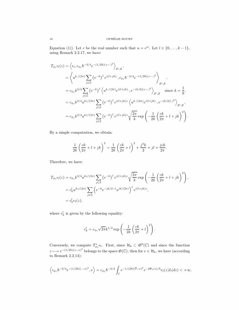
Equation (1)). Let c be the real number such that u = eic. Let l ∈ {0, . . . , k − 1},using Remark 2.2.17, we have:

Tφ1ǫl(z) =

⟨

ǫl, cφ1~−3/4e−(1/2~)(z−.)2

⟩

S′,S,

=

⟨

uk./(2π)∑

j∈Z

(

v−k)jei(l+jk)., cφ1

~−3/4e−(1/2~)(z−.)2

⟩

S′,S

,

= cφ1k3/4

∑

j∈Z

(

v−k)j⟨

uk./(2π)ei(l+jk)., e−(k/2)(z−.)2⟩

S′,Ssince k =

1

~,

= cφ1k3/4ukz/(2π)

∑

j∈Z

(

v−k)jei(l+jk)z

⟨

uk./(2π)ei(l+jk)., e−(k/2)(.)2⟩

S′,S,

= cφ1k3/4ukz/(2π)

∑

j∈Z

(

v−k)jei(l+jk)z

√

2π

kexp

(

− 1

2k

(

ck

2π+ l + jk

)2)

.

By a simple computation, we obtain:

1

2k

(

ck

2π+ l + jk

)2

=1

2k

(

ck

2π+ l

)2

+j2k

2+ jl +

jck

2π.

Therefore, we have:

Tφ1ǫl(z) = cφ1

k3/4ukz/(2π)∑

j∈Z

(

v−k)jei(l+jk)z

√

2π

kexp

(

− 1

2k

(

ck

2π+ l + jk

)2)

,

= clkukz/(2π)

∑

j∈Z

(

v−ke−jk/2−luik/(2π))j

ei(l+jk)z ,

= clkel(z),

where clk is given by the following equality:

clk = cφ1

√2πk1/4 exp

(

− 1

2k

(

ck

2π+ l

)2)

.

Conversely, we compute T ∗φ1el. First, since Hk ⊂ S

0(C) and since the function

z 7−→ e−(1/2~)(z−x)2 belongs to the space S(C), then for v ∈ Hk, we have (accordingto Remark 2.2.14):

⟨

cφ1~−3/4e−(1/2~)(.−x)2, v

⟩

= cφ1~−3/4

∫

C

e−1/(2~)(z−x)2e−2Φ1(z)/~el(z)L(dz) < +∞.


Let l ∈ {0, 1, . . . , k − 1}, then we have:

T ∗φ1el(x)

= cφ1~−3/4

∫

C

e−1/(2~)(z−x)2e−2Φ1(z)/~el(z)L(dz),

= cφ1k3/4

∫

C

e−(k/2)(z−x)2e−k(ℑz)2

el(z)L(dz) because Φ1(z) =1

2(ℑz)2 and k =

1

~,

= cφ1k3/4

∫

C

e−(k/2)(z−x)2e−k(ℑz)2

ukz/(2π)∑

j∈Z

(

v−ke−l−jk/2uik/(2π))j

ei(l+jk)zL(dz),

= cφ1k3/4

∑

j∈Z

(

v−ke−l−jk/2uik/(2π))j∫

C

e−(k/2)(z)2e−k(ℑ(z+x))2uk(z+x)/(2π)ei(l+jk)(z+x)L(dz),

= cφ1k3/4ukx/(2π)

∑

j∈Z

(


ei(l+jk)x∫

C

e−(k/2)(z)2e−k(ℑz)2

eiz(l+jk+ck/(2π))L(dz).

We have to compute the following integral (after the change of variables z = p+iq):∫

R

∫

R

e−(k/2)(p−iq)2e−kq2

ei(p+iq)(l+jk+ck/(2π))dpdq

=

∫

R

∫

R

e−kp2/2e−kq

2/2eikpqeip(l+jk+ck/(2π))e−q(l+jk+ck/(2π))dpdq.

By a simple computation, we obtain:

∫

R

e−kp2/2eikpqeip(l+jk+ck/(2π))dp =

√

2π

kexp

(

− 1

2k

(

l+ jk +ck

2π

)2

− kq2

2− q

(

l + jk +ck

2π

)

)

.

Thus, by an other simple computation, we obtain:∫

R

∫

R

e−kp2/2e−kq

2/2eikpqeip(l+jk+ck/(2π))e−q(l+jk+ck/(2π))dpdq =√2π

ke(l+jk+ck/(2π))

2/(2k).

Consequently, we obtain:

T ∗φ1el(x)

= cφ1k3/4

√2π

kukx/(2π)

∑

j∈Z

(


ei(l+jk)xe(l+jk+ck/(2π))2/(2k),

= cφ1k−1/4

√2πe(l+ck/(2π))

2/(2k)ukx/(2π)∑

j∈Z

(

v−k)jei(l+jk)x,

= clkǫl(x),

where clk = cφ1k−1/4

√2πe(l+ck/(2π))

2/(2k). �

Since the Bargmann transform is a unitary transformation between the spacesL2(R) and H~(C,Φ1), we study this feature between the spaces Lk and Hk.

Proposition 2.2.19.

(1) T ∗φ1Tφ1

= id on Lk.(2) Tφ1

T ∗φ1

= id on Hk.

18 OPHÉLIE ROUBY

Proof. Let c be the real number such that u = eic. According to the proof ofProposition 2.2.18, we have, for l ∈ {0, . . . , k − 1}:

Tφ1ǫl = clkel with clk = cφ1

√2πk1/4e−(ck/(2π)+l)2/(2k).

Let C = diag(c0k, . . . , ck−1k ) be the matrix of the operator Tφ1

in the basis (el)l∈Z/kZ.According to the proof of Proposition 2.2.18, we also have, for l ∈ {0, . . . , k − 1}:

T ∗φ1el = clkǫl with clk = cφ1

k−1/4√2πe(l+ck/(2π))

2/(2k).

Let C∗ = diag(c0k, . . . , ck−1k ) be the matrix of the operator T ∗

φ1in the basis (ǫl)l∈Z/kZ.

We want to prove that: CC∗ = C∗C = Ik. Let k ≥ 1 and let l ∈ {0, 1, . . . , k− 1}, wehave:

clk clk = cφ1

√2πk1/4e−(ck/(2π)+l)2/(2k)cφ1

k−1/4√2πe(l+ck/(2π))

2/(2k),

= c2φ12π3/2,

=

(

1

21/2π3/4

)2

2π3/2 according to Definition 2.2.8,

= 1,

= clkclk.

Therefore, we have: CC∗ = C∗C = Ik. �

2.2.3. Complex Weyl quantization of the torus. In this paragraph, we define thecomplex Weyl quantization of a symbol on the torus. As in the classical Weylquantization case, we have two definitions for the complex Weyl quantization. Withan Egorov theorem analogous to Proposition 2.2.10 in the R2-case, we exhibit thenotion of complex Weyl quantization of the torus. First, we introduce a new classof symbols. Recall that ΛΦ1

denotes the following space:

ΛΦ1=

{(

z,2

i

∂Φ1

∂z(z)

)

; z ∈ C

}

= {(z,−ℑ(z)); z ∈ C} .

And that the canonical transformation κφ1is defined as follows:

κφ1: R2 −→ ΛΦ1

(x, y) 7−→ (z, w) := (x− iy, y).

Notice that, if ak ∈ C∞k (R2) is a function such that, for all (x, y) ∈ R2, we have:

ak(x + 2π, y) = ak(x, y) = ak(x, y + 1);

and if bk is the function defined by the following relation, for (z, w) ∈ ΛΦ1:

bk(z, w) := ak ◦ κ−1φ1

(z, w).

Then bk ∈ C∞k (ΛΦ1

) is a function such that, for (z, w) ∈ ΛΦ1, we have:

bk(z + 2π,w) = bk(z, w) = bk(z + i, w − 1).

Besides, thanks to the identification of ΛΦ1with C, we can rewrite the symbol bk

as a convergent series, for z ∈ C ≃ ΛΦ1:

(8) bk(z) =∑

(m,n)∈Z2

bkm,neinℜ(z)e2iπmℑ(z),


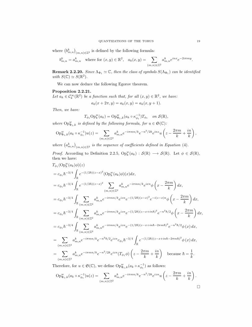
where(

bkm,n)

(m,n)∈Z2is defined by the following formula:

bkm,n = akm,n where for (x, y) ∈ R2, ak(x, y) =

∑

(m,n)∈Z2

akm,neinxe−2iπmy.

Remark 2.2.20. Since ΛΦ1≃ C, then the class of symbols S(ΛΦ1

) can be identifiedwith S(C) ≃ S(R2).

We can now deduce the following Egorov theorem.

Proposition 2.2.21.

Let ak ∈ C∞k (R2) be a function such that, for all (x, y) ∈ R2, we have:

ak(x + 2π, y) = ak(x, y) = ak(x, y + 1).

Then, we have:

Tφ1Opwk (ak) = OpwΦ1,k(ak ◦ κ

−1φ1

)Tφ1on S(R),

where OpwΦ1,k is defined by the following formula, for u ∈ S(C):

OpwΦ1,k(ak ◦ κ−1φ1

)u(z) =∑

(m,n)∈Z2

akm,ne−iπmn/ke−n

2/2keinzu

(

z − 2πm

k+in

k

)

,

where(

akm,n)

(m,n)∈Z2is the sequence of coefficients defined in Equation (4).

Proof. According to Definition 2.2.5, Opwk (ak) : S(R) −→ S(R). Let φ ∈ S(R),then we have:

Tφ1(Opwk (ak)φ)(z)

= cφ1~−3/4

∫

R

e−(1/2~)(z−x)2(Opwk (ak)φ)(x)dx,

= cφ1~−3/4

∫

R

e−(1/2~)(z−x)2∑

(m,n)∈Z2

akm,ne−iπmn/keixnφ

(

x− 2πm

k

)

dx,

= cφ1~−3/4

∫

R

∑

(m,n)∈Z2

akm,ne−iπmn/keizne−(1/2~)(z−x)2e−i(z−x)nφ

(

x− 2πm

k

)

dx,

= cφ1~−3/4

∫

R

∑

(m,n)∈Z2

akm,ne−iπmn/keizne−(1/2~)(z−x+in~)2e−n

2~/2φ

(

x− 2πm

k

)

dx,

= cφ1~−3/4

∫

R

∑

(m,n)∈Z2

akm,ne−iπmn/keizne−(1/2~)(z−x+in~−2πm~)2e−n

2~/2φ (x) dx,

=∑

(m,n)∈Z2


2~/2eizncφ1

~−3/4

∫

R

e−(1/2~)(z−x+in~−2πm~)2φ (x) dx,

=∑

(m,n)∈Z2


2/2keizn(Tφ1φ)

(

z − 2πm

k+in

k

)

because ~ =1

k.

Therefore, for u ∈ S(C), we define OpwΦ1,k(ak ◦ κ−1φ1

) as follows:

OpwΦ1,k(ak ◦ κ−1φ1

)u(z) =∑

(m,n)∈Z2


2/2keiznu

(

z − 2πm

k+in

k

)

.

�

20 OPHÉLIE ROUBY

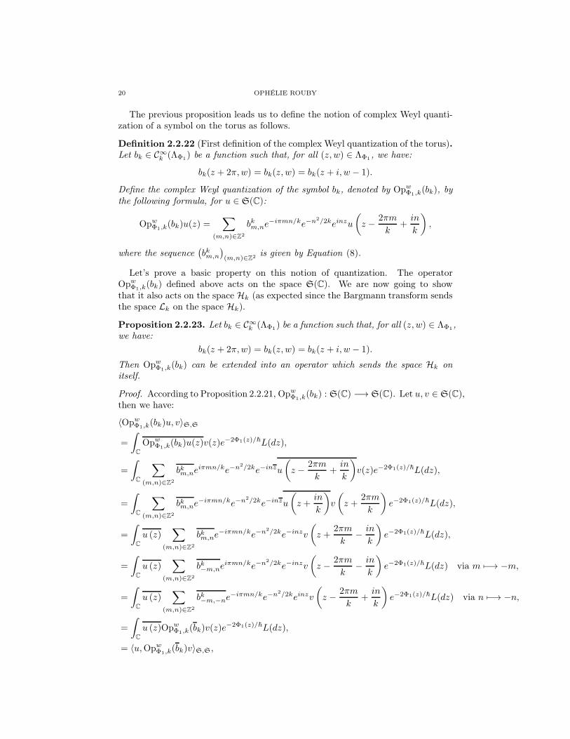
The previous proposition leads us to define the notion of complex Weyl quanti-zation of a symbol on the torus as follows.

Definition 2.2.22 (First definition of the complex Weyl quantization of the torus).Let bk ∈ C∞

k (ΛΦ1) be a function such that, for all (z, w) ∈ ΛΦ1

, we have:

bk(z + 2π,w) = bk(z, w) = bk(z + i, w − 1).

Define the complex Weyl quantization of the symbol bk, denoted by OpwΦ1,k(bk), bythe following formula, for u ∈ S(C):

OpwΦ1,k(bk)u(z) =∑

(m,n)∈Z2

bkm,ne−iπmn/ke−n

2/2keinzu

(

z − 2πm

k+in

k

)

,

where the sequence(

bkm,n)

(m,n)∈Z2is given by Equation (8).

Let’s prove a basic property on this notion of quantization. The operatorOpwΦ1,k(bk) defined above acts on the space S(C). We are now going to showthat it also acts on the space Hk (as expected since the Bargmann transform sendsthe space Lk on the space Hk).

Proposition 2.2.23. Let bk ∈ C∞k (ΛΦ1

) be a function such that, for all (z, w) ∈ ΛΦ1,

we have:

bk(z + 2π,w) = bk(z, w) = bk(z + i, w − 1).

Then OpwΦ1,k(bk) can be extended into an operator which sends the space Hk onitself.

Proof. According to Proposition 2.2.21, OpwΦ1,k(bk) : S(C) −→ S(C). Let u, v ∈ S(C),then we have:

〈OpwΦ1,k(bk)u, v〉S,S

=

∫

C

OpwΦ1,k(bk)u(z)v(z)e−2Φ1(z)/~L(dz),

=

∫

C

∑

(m,n)∈Z2

bkm,neiπmn/ke−n

2/2ke−inzu

(

z − 2πm

k+in

k

)

v(z)e−2Φ1(z)/~L(dz),

=

∫

C

∑

(m,n)∈Z2


2/2ke−inzu

(

z +in

k

)

v

(

z +2πm

k

)

e−2Φ1(z)/~L(dz),

=

∫

C

u (z)∑

(m,n)∈Z2


2/2ke−inzv

(

z +2πm

k− in

k

)

e−2Φ1(z)/~L(dz),

=

∫

C

u (z)∑

(m,n)∈Z2

bk−m,neiπmn/ke−n

2/2ke−inzv

(

z − 2πm

k− in

k

)

e−2Φ1(z)/~L(dz) via m 7−→ −m,

=

∫

C

u (z)∑

(m,n)∈Z2

bk−m,−ne−iπmn/ke−n

2/2keinzv

(

z − 2πm

k+in

k

)

e−2Φ1(z)/~L(dz) via n 7−→ −n,

=

∫

C

u (z)OpwΦ1,k(bk)v(z)e−2Φ1(z)/~L(dz),

= 〈u,OpwΦ1,k(bk)v〉S,S,


where bk ∈ C∞k (ΛΦ1

) is defined, for (z, w) ∈ ΛΦ1, by:

bk(z, w) =∑

(m,n)∈Z2

bk−m,−nein(z+iw)e−2iπmw,

=∑

(m,n)∈Z2

bkm,ne−in(z+iw)e2iπmw via (m,n) 7−→ (−m,−n),

=∑

(m,n)∈Z2

bkm,ne−inℜ(z)e−2iπmℑ(z) because (z, w) ∈ ΛΦ1

, thus w = −ℑ(z),

= bk(z, w).

Since v ∈ S(C) and bk ∈ C∞k (ΛΦ1

), then OpwΦ1,k(bk)v ∈ S(C) and the complexWeyl quantization OpwΦ1,k(bk) is well-defined on S

′(C) by the following formula,for u ∈ S

′(C) and for v ∈ S(C):

〈OpwΦ1,k(bk)u, v〉S′,S := 〈u,OpwΦ1,k(bk)v〉S′,S.

Afterwards, since Hk ⊂ S′(C), then for g ∈ Hk, OpwΦ1,k(bk)g ∈ Hol(C). Moreover,

for g ∈ Hk, using simple computations we prove that:{

OpwΦ1,k(bk)g(z + 2π) = ukOpwΦ1,k(bk)g(z),

OpwΦ1,k(bk)g(z + i) = vke−ikz+k/2OpwΦ1,k(bk)g(z).

�

Let’s give a second definition of the complex Weyl quantization of the torus.This notion is analogous to the already existing one in the R2-case (see for example[HS15] or [Zwo12]). We believe that it is the first time that such a contour integralis used in a context of the quantization of a compact phase space.

Definition 2.2.24 (Second definition of the complex Weyl quantization of thetorus). Let b~ ∈ C∞

~(ΛΦ1

) be a function such that, for all (z, w) ∈ ΛΦ1, we have:

b~(z + 2π,w) = b~(z, w) = b~(z + i, w − 1).

Define the complex Weyl quantization of the symbol b~, denoted by OpwΦ1(b~), by

the following formula, for u ∈ S(C):

OpwΦ1(b~)u(z) =

1

2π~

∫∫

Γ(z)

e(i/~)(z−w)ζb~

(

z + w

2, ζ

)

u(w)dwdζ,


Γ(z) =

{

(w, ζ) ∈ C2; ζ =

2

i

∂Φ1

∂z

(

z + w

2

)

= −ℑ(

z + w

2

)}

.

This second definition expresses the fact that the complex Weyl quantization ofR2 (seen in Proposition 2.2.10) can be extended to a symbol defined on the torus.Similarly to Proposition 2.2.23, we have the following property.

Proposition 2.2.25. Let b~ ∈ C∞~(ΛΦ1

) be a function such that, for all (z, w) ∈ ΛΦ1,

we have:

b~(z + 2π,w) = b~(z, w) = b~(z + i, w − 1).

Then, OpwΦ1(b~) can be extended into an operator which sends Hk on itself.

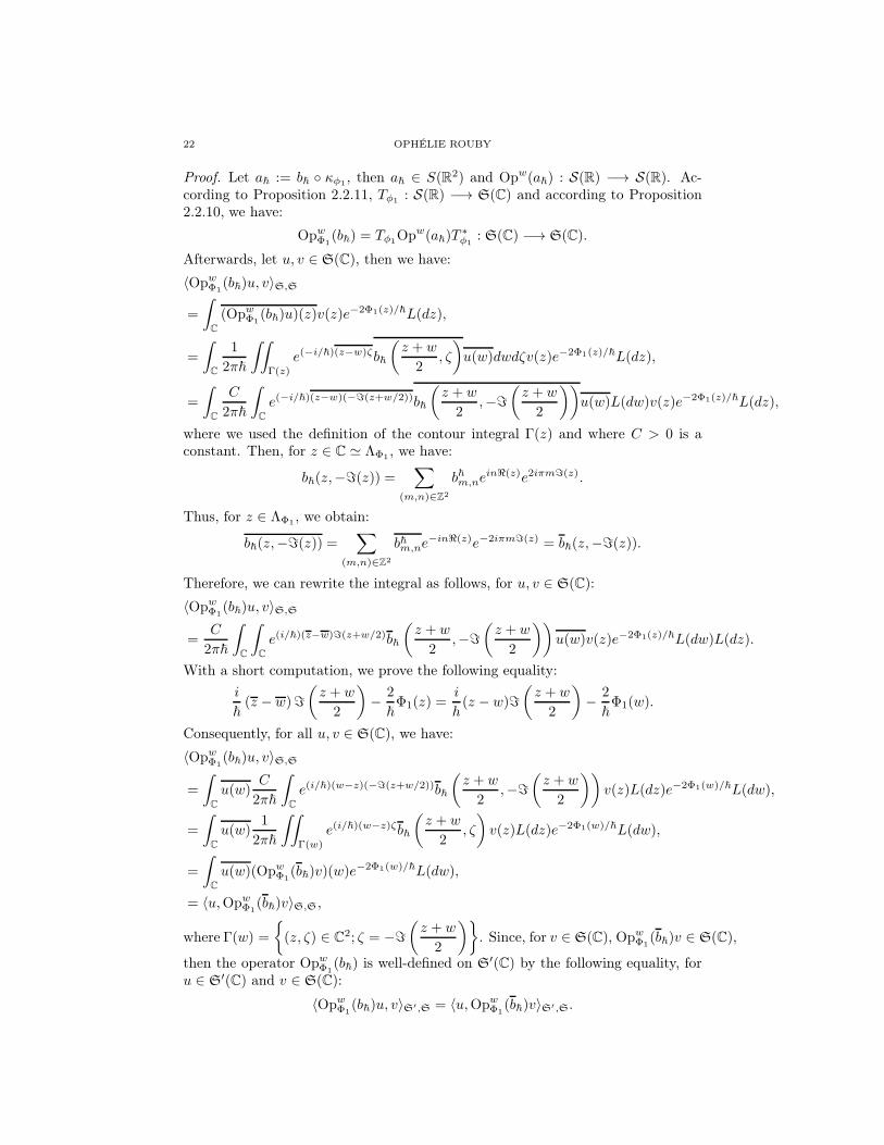
22 OPHÉLIE ROUBY

Proof. Let a~ := b~ ◦ κφ1, then a~ ∈ S(R2) and Opw(a~) : S(R) −→ S(R). Ac-

cording to Proposition 2.2.11, Tφ1: S(R) −→ S(C) and according to Proposition

2.2.10, we have:

OpwΦ1(b~) = Tφ1

Opw(a~)T∗φ1

: S(C) −→ S(C).

Afterwards, let u, v ∈ S(C), then we have:

〈OpwΦ1(b~)u, v〉S,S

=

∫

C

(OpwΦ1(b~)u)(z)v(z)e

−2Φ1(z)/~L(dz),

=

∫

C

1

2π~

∫∫

Γ(z)

e(−i/~)(z−w)ζb~

(

z + w

2, ζ

)

u(w)dwdζv(z)e−2Φ1(z)/~L(dz),

=

∫

C

C

2π~

∫

C

e(−i/~)(z−w)(−ℑ(z+w/2))b~

(

z + w

2,−ℑ

(

z + w

2

))

u(w)L(dw)v(z)e−2Φ1(z)/~L(dz),

where we used the definition of the contour integral Γ(z) and where C > 0 is aconstant. Then, for z ∈ C ≃ ΛΦ1

, we have:

b~(z,−ℑ(z)) =∑

(m,n)∈Z2

b~m,neinℜ(z)e2iπmℑ(z).

Thus, for z ∈ ΛΦ1, we obtain:

b~(z,−ℑ(z)) =∑

(m,n)∈Z2

b~m,ne−inℜ(z)e−2iπmℑ(z) = b~(z,−ℑ(z)).

Therefore, we can rewrite the integral as follows, for u, v ∈ S(C):


=C

2π~

∫

C

∫

C

e(i/~)(z−w)ℑ(z+w/2)b~

(

z + w

2,−ℑ

(

z + w

2

))

u(w)v(z)e−2Φ1(z)/~L(dw)L(dz).

With a short computation, we prove the following equality:

i

~(z − w)ℑ

(

z + w

2

)

− 2

~Φ1(z) =

i

h(z − w)ℑ

(

z + w

2

)

− 2

~Φ1(w).

Consequently, for all u, v ∈ S(C), we have:


=

∫

C

u(w)C

2π~

∫

C

e(i/~)(w−z)(−ℑ(z+w/2))b~

(

z + w

2,−ℑ

(

z + w

2

))

v(z)L(dz)e−2Φ1(w)/~L(dw),

=

∫

C

u(w)1

2π~

∫∫

Γ(w)

e(i/~)(w−z)ζb~

(

z + w

2, ζ

)

v(z)L(dz)e−2Φ1(w)/~L(dw),

=

∫

C

u(w)(OpwΦ1(b~)v)(w)e

−2Φ1(w)/~L(dw),

= 〈u,OpwΦ1(b~)v〉S,S,

where Γ(w) =

{

(z, ζ) ∈ C2; ζ = −ℑ(

z + w

2

)}

. Since, for v ∈ S(C), OpwΦ1(b~)v ∈ S(C),

then the operator OpwΦ1(b~) is well-defined on S

′(C) by the following equality, foru ∈ S

′(C) and v ∈ S(C):

〈OpwΦ1(b~)u, v〉S′,S = 〈u,OpwΦ1

(b~)v〉S′,S.


As a result, the operator OpwΦ1(b~) is well-defined on Hk because it is a sub-

space of S′(C). Afterwards, since for g ∈ Hk, OpwΦ1(b~)g ∈ S

′(C), then we haveOpwΦ1

(b~)g ∈ Hol(C). Besides using simple computations, for g ∈ Hk, we provethat:

{

OpwΦ1(b~)g(z + 2π) = ukOpwΦ1

(b~)g(z),

OpwΦ1(b~)g(z + i) = vke−ikz+k/2OpwΦ1

(b~)g(z).

�

To conclude this paragraph, we link Definition 2.2.22 and Definition 2.2.24.

Proposition 2.2.26. Let b~ = bk ∈ C∞~(ΛΦ1

) be a function such that, for all(z, w) ∈ ΛΦ1

, we have:

b~(z + 2π,w) = b~(z, w) = b~(z + i, w − 1).

Then:

OpwΦ1(b~) = OpwΦ1,k(bk) on Hk.

Proof. According to Equation (8), for (z, w) ∈ ΛΦ1, we can rewrite b~ as follows:

b~(z, w) =∑

(m,n)∈Z2

b~m,nein(z+iw)e−2iπmw.

Consequently, we obtain, for u ∈ S(C):

OpwΦ1(b~)u(z)

=1

2π~

∫∫

Γ(z)

e(i/~)(z−w)ζ∑

(m,n)∈Z2

b~m,nein((z+w)/2+iζ)e−2iπmζu(w)dwdζ,

=1

2π~

∫∫

Γ(z)

∑

(m,n)∈Z2

e(i/~)(z−w)ζb~m,nein((z+w)/2+iζ)e−iπmn/ku

(

w − 2πm

k

)

dwdζ,

=1

2π~

∫∫

Γ(z)

e(i/~)(z−w)ζ∑

(m,n)∈Z2

b~m,ne−iπmn/ke−n

2/2ku

(

w +in

k− 2πm

k

)

dwdζ,

=1

2π~

∫∫

Γ(z)

e(i/~)(z−w)ζ(OpwΦ1,k(bk)u)(w)dwdζ,

= OpwΦ1,k(bk)u(z),

where we used the change of variables: Γ(z) ∋ (w, ζ) 7−→(

w +in

k, ζ − n

2k

)

∈ Γ(z).

Therefore, for u ∈ S′(C) and v ∈ S(C), we have:

〈OpwΦ1(b~)u, v〉S′,S = 〈u,OpwΦ1

(b~)v〉S′,S,

= 〈u,OpwΦ1,k(bk)v〉S′,S,

= 〈OpwΦ1,k(bk)u, v〉S′,S.

In others words, we have:

OpwΦ1(b~) = OpwΦ1,k(bk) on S

′(C).

Finally, since Hk ⊂ S′(C), then by restriction and according to Propositions 2.2.23

and 2.2.25, we obtain the result. �

24 OPHÉLIE ROUBY

2.3. Connections between the quantizations of the torus T2. In this para-graph, we relate the different notions of quantization of the torus. To do so, wefollow these steps:

1. we recall the connection between a Berezin-Toeplitz operator and a complexpseudo-differential operator of the complex plane;

2. within the Berezin-Toeplitz setting, we relate the quantization of the torusto the quantization of the complex plane;

3. we establish a correspondence between the Berezin-Toeplitz and the com-plex Weyl quantizations of the torus.

2.3.1. Berezin-Toeplitz and complex Weyl quantizations of the complex plane. First,we recall the definition of the Berezin-Toeplitz quantization of a symbol on thecomplex plane and then the definition of the complex Weyl quantization of a symbolon ΛΦ1

(see for example [Zwo12]).

Definition 2.3.1 (Berezin-Toeplitz quantization of the complex plane). Let fk ∈ S(C)be a function admitting an asymptotic expansion in powers of 1/k. Define theBerezin-Toeplitz quantization of fk by the sequence of operators Tfk := (Tk)k≥1,where for k ≥ 1, Tk is defined by:

Tk = ΠΦ1,kMfkΠΦ1,k,

where Mfk : L2k(C,Φ1) −→ L2

k(C,Φ1) is the multiplication operator by the functionfk and where we recall that ΠΦ1,k is the orthogonal projection of the space L2

k(C,Φ1)on Hk(C,Φ1) defined in Proposition 2.2.9.We call fk the symbol of the Berezin-Toeplitz operator Tfk .

Definition 2.3.2 (Complex Weyl quantization of the complex plane). Let b~ ∈ S(ΛΦ1)

be a function admitting an asymptotic expansion in powers of ~. Define the com-plex Weyl quantization of b~, denoted by OpwΦ1

(b~), by the following formula, foru ∈ H~(C,Φ1):

OpwΦ1(b~)u(z) =

1

2π~

∫∫

Γ(z)

e(i/~)(z−w)ζb~

(

z + w

2, ζ

)

u(w)dwdζ,


Γ(z) =

{

(w, ζ) ∈ C2; ζ =

2

i

∂Φ1

∂z

(

z + w

2

)

= −ℑ(

z + w

2

)}

.

Recall now the result relating these two quantizations (see for example [Zwo12,Chapter 13]).

Proposition 2.3.3.

(1) Let fk ∈ S(C) be a function admitting an asymptotic expansion in powersof 1/k. Let Tfk = (Tk)k≥1 be the Berezin-Toeplitz operator of symbol fk.Then, for k ≥ 1, we have:

Tk = OpwΦ1(b~) on Hk(C,Φ1),

where b~ ∈ S(ΛΦ1) is a function admitting an asymptotic expansion in

powers of ~ given by the following formula, for all z ∈ ΛΦ1≃ C:

b~(z) = exp

(

1

k∂z∂z

)

(fk(z)).


(2) Let b~ ∈ S(ΛΦ1) be a function admitting an asymptotic expansion in powers

of ~. Then, there exists fk ∈ S(C) a function admitting an asymptoticexpansion in powers of 1/k such that for k ≥ 1:

OpwΦ1(b~) = Tk +O(k−∞) on H~(C,Φ1),

where (Tk)k≥1 = Tfk is the Berezin-Toeplitz operator of symbol fk andwhere, for all N ∈ N and for z ∈ C, fk is given by:

fk(z) =

N∑

j=0

~j

j!(DzDz)

j(b~(z)) +O(~N+1).

2.3.2. Berezin-Toeplitz quantization of the torus and Berezin-Toeplitz quantizationof the complex plane. In this paragraph, we study a Berezin-Toeplitz operator ofthe complex plane whose symbol is 2π-periodic with respect to its first variable and1-periodic with respect to its second variable. Previously, we looked at the actionof a Berezin-Toeplitz operator of the complex plane on the spaces S(C) and S

′(C).

Proposition 2.3.4. Let fk ∈ S(C) be a function admitting an asymptotic expan-sion in powers of 1/k. Let Tfk = (Tk)k≥1 be the Berezin-Toeplitz operator of symbolfk. Then, for k ≥ 1, we have:

(1) Tk can be defined as an operator which sends S(C) on itself by:

Tkv = ΠΦ1,k(fkv) for v ∈ S(C),

where ΠΦ1,k is seen as an operator which sends S(C) on itself.(2) Tk can be extended into an operator which sends S

′(C) on itself by:

〈Tku, v〉S′,S = 〈u, Tkv〉S′,S for u ∈ S′(C) and for v ∈ S(C),

where (Tk)k≥1 =: Tfk

is the Berezin-Toeplitz operator of symbol fk.

Proof. Since Tfk = (Tk)k≥1 is a Berezin-Toeplitz operator of the complex plane,then according to Proposition 2.3.3, there exists b~ ∈ S(ΛΦ1

) such that, for k ≥ 1:

Tk = OpwΦ1(b~) on Hk(C,Φ1).

Besides, according to Proposition 2.2.10, we know that:

T ∗φ1OpwΦ1

(b~)Tφ1= Opw(b~ ◦ κφ1

) : L2(R) −→ L2(R).

Since b~ ◦ κφ1∈ S(R2), then we have:

Opw(b~ ◦ κφ1) : S(R) −→ S(R) and Opw(b~ ◦ κφ1

) : S ′(R) −→ S ′(R).

Moreover, according to Propositions 2.2.11, 2.2.13 and 2.2.16, the Bargmann trans-form and its adjoint satisfy:

{

Tφ1: S(R) −→ S(C) and T ∗

φ1: S(C) −→ S(R),

Tφ1: S ′(R) −→ S

′(C) and T ∗φ1

: S′(C) −→ S ′(R).

As a result, for k ≥ 1, we obtain:

Tk : S(C) −→ S(C) and Tk : S′(C) −→ S′(C).

Then, by definition ΠΦ1,k = Tφ1T ∗φ1

and according to Proposition 2.2.11, the op-

erator ΠΦ1,k can be extended into an operator which sends S(C) on itself. SinceS(C) ⊂ H~(C,Φ1) (see Remark 2.2.12), then for v ∈ S(C) and for fk ∈ S(C), wehave:

ΠΦ1,kv = v and ΠΦ1,k(fkv) ∈ S(C).

26 OPHÉLIE ROUBY

Therefore, the Berezin-Toeplitz operator Tfk = (Tk)k≥1 is defined as follows, fork ≥ 1 and for v ∈ S(C):

Tkv = ΠΦ1,kMfkΠΦ1,kv = ΠΦ1,k(fkv),

whereΠΦ1,k is an operator which sends S(C) on itself. Finally, for v = Tφ1ψ ∈ S

′(C)and for u = Tφ1

φ ∈ S(C), we have:

〈Tkv, u〉S′,S = 〈OpwΦ1(b~)v, u〉S′,S according to Proposition 2.3.3,

= 〈v,OpwΦ1(b~)u〉S′,S according to Proposition 2.2.25,

=: 〈v, Tku〉S′,S.

Then, according to Proposition 2.3.3, for z ∈ ΛΦ1≃ C, we have:

b~(z) = exp

(

1

k∂z∂z

)

(fk(z)).

Consequently, for z ∈ ΛΦ1≃ C, we obtain:

b~(z) = exp

(

1

k∂z∂z

)

(fk(z)).

In others words, the sequence of operators (Tk)k≥1 is a Berezin-Toeplitz operator

of symbol fk. �

Remark 2.3.5. Let fk ∈ C∞k (R2) be a function such that, for (x, y) ∈ R2, we have:

fk(x+ 2π, y) = fk(x, y) = fk(x, y + 1).

Let Tfk = (Tk)k≥1 be the Berezin-Toeplitz operator of the complex plane of symbolfk. Then, for k ≥ 1, the operator Tk is well-defined on Hk according to Proposition2.3.4 since Hk ⊂ S

′(C).

The following proposition gives a connection between the orthogonal projectionΠΦ1,k which appears in the definition of a Berezin-Toeplitz operator of the complexplane (see Definition 2.3.1) and the orthogonal projection Πk which appears inthe definition of a Berezin-Toeplitz operator of the torus (see Definition 1.1.3).This proposition is fundamental for understanding the relation between these twoquantizations.

Proposition 2.3.6.

Let ΠΦ1,k be the orthogonal projection of L2k(C,Φ1) on Hk(C,Φ1). Then:

(1) ΠΦ1,k can be extended into an operator which sends Gk on Hk (defined inSubsection 1.1);

(2) ΠΦ1,k = id on Hk.

Consequently, ΠΦ1,k coincides with Πk on Gk.

Proof. First, let’s prove that ΠΦ1,k is well-defined on Gk. The main difficulty toprove this result comes from the fact that Gk is not included in S

′(C). Recall theformula defining ΠΦ1,k for g ∈ L2

k(C,Φ1) (see Proposition 2.2.9):

ΠΦ1,kg(z) =

∫

C

e−(1/4~)(z−w)2g(w)e−2Φ1(w)/~L(dw).


Let g ∈ Gk, by a simple computation, we notice that, for (m,n) ∈ Z2 and for z ∈ C,we have:

g(z + 2πm) =(

uk)m

g(z),

g(z + in) =(

vke−izk+kn/2)n

g(z).

Then, for g ∈ Gk, we can write an estimate of the integral defining ΠΦ1,k as follows:∫

C

∣

∣

∣e−(1/4~)(z−w)2g(w)e−2Φ1(w)/~

∣

∣

∣L(dw),

=∑

m∈Z

∫

[0,2π]+iR

∣

∣

∣e−(1/4~)(z−(w+2πm))2g(w + 2πm)e−2Φ1(w+2πm)/~

∣

∣

∣L(dw),

=∑

m∈Z

∫

[0,2π]+iR

∣

∣

∣e−(1/4~)(z−w−2πm)2

(

uk)m

g(w)e−2Φ1(w)/~∣

∣

∣L(dw),

=∑

(m,n)∈Z2

∫

[0,2π]+i[0,1]

∣

∣

∣e−(1/4~)(z−(w+in)−2πm)2

(

uk)m

g(w + in)e−2Φ1(w+in)/~∣

∣

∣L(dw),

=∑

(m,n)∈Z2

∫

[0,2π]+i[0,1]

∣

∣

∣e−(1/4~)(z−w+in−2πm)2

(

uk)m(

vke−iwk+kn/2)n

g(w)

e−2Φ1(w)/~e−n2/~e−2nℑ(w)/~

∣

∣

∣L(dw),

=∑

(m,n)∈Z2

∫

[0,2π]+i[0,1]

∣

∣

∣e−(1/4~)(z−w+in−2πm)2

(

uk)m (

vk)ne−kn

2/2e−inkwg(w)e−2Φ1(w)/~∣

∣

∣L(dw).

For all z ∈ C, we have:∫

[0,2π]+i[0,1]

∣

∣

∣e−(1/4~)(z−w+in−2πm)2

(

uk)m (

vk)ne−kn


∣

∣L(dw)

=

∫

[0,2π]+i[0,1]

∣

∣

∣e−(1/4~)(z−w+in−2πm)2e−kn


∣

∣L(dw)

≤ ‖g‖2Gk

∫

[0,2π]+i[0,1]

∣

∣

∣e−(1/4~)(z−w+in−2πm)2e−kn

2/2e−inkw∣

∣

∣

2

e−2Φ1(w)/~L(dw)

using Cauchy-Schwartz in L2([0, 2π] + i[0, 1], e−2Φ1(z)/~L(dz)),

= ‖g‖2Gk

∫

[0,2π]+i[0,1]

∣

∣

∣e−(1/4~)(z−w+in−2πm)2e−inkw

∣

∣

∣

2

e−kn2

e−2Φ1(w)/~L(dw),

≤ C‖g‖2Gke−kℜ(z2)/2e−2kπ2m2

e−kn2/2 max

(

e2πmkℜ(z), e2π(m+1)kℜ(z))

max(

enkℑ(z), e(n+1)kℑ(z))

,

where C is a constant independent of k. We recognize the general term of a con-vergent series in m and n, thus according to Fubini’s theorem, ΠΦ1,k is well-definedon Gk by the following formula, for g ∈ Gk:

ΠΦ1,kg(z) =

∫

C

e−(1/4~)(z−w)2g(w)e−2Φ1(w)/~L(dw),

=∑

(m,n)∈Z2

∫

[0,2π]+i[0,1]

e−(1/4~)(z−w+in−2πm)2(

uk)m (

vk)ne−kn

2/2e−inkwg(w)e−2Φ1(w)/~L(dw).

Now, since the range of ΠΦ1,k consists of holomorphic functions, then for g ∈ Gk,ΠΦ1,kg ∈ Hol(C). Then, via the change of variables w 7−→ w + 2π, we prove with

28 OPHÉLIE ROUBY

simple integral equalities that, for g ∈ Gk, we have ΠΦ1,kg(z + 2π) = ukΠΦ1,kg(z)and using the change of variables w 7−→ w + i, we also obtain that, for g ∈ Gk,ΠΦ1,kg(z + i) = vke−ikz+k/2ΠΦ1,kg(z). Finally, we recall that ΠΦ1,k = id on Hk

comes from Proposition 2.2.19. �

We can now define the action of a Berezin-Toeplitz operator of the complex planeon the space Hk.

Proposition 2.3.7. Let fk ∈ C∞k (C) be a function such that, for z ∈ C, we have:

fk(z + 2π) = fk(z) = fk(z + i).

Let Tfk = (Tk)k≥1 be the Berezin-Toeplitz operator of the complex plane of symbolfk. Then, for k ≥ 1 and for v ∈ Hk, we have:

Tkv = ΠΦ1,k(fkv),

where ΠΦ1,k is seen as the operator which sends Gk on Hk (see Proposition 2.3.6).

Proof. According to Proposition 2.3.4, for v ∈ Hk, for u ∈ S(C) and for k ≥ 1, wehave:

〈Tkv, u〉S′,S = 〈v, Tku〉S′,S,

= 〈g, Tku〉 with g ∈ S−l(C) for l ∈ N according to Proposition 2.2.15,

= 〈g,ΠΦ1,kMfk

ΠΦ1,ku〉 by definition of Tk on S(C),

= 〈ΠΦ1,kMfk

ΠΦ1,kg, u〉 since Π∗Φ1,k = ΠΦ1,k.

Thus, for v ∈ Hk and for k ≥ 1, we obtain, according to Proposition 2.3.6:

Tkv = ΠΦ1,kMfkΠΦ1,kv = ΠΦ1,k(fkv).

�

We deduce from Proposition 2.3.7 and Proposition 2.3.6, a result which relatesa Berezin-Toeplitz operator of the complex plane and a Berezin-Toeplitz operatorof the torus. To our knowledge, this fact is new in the literature and it is alsofundamental to prove Theorem A.

Proposition 2.3.8. Let fk ∈ C∞k (C) be a function such that, for z ∈ C, we have:

fk(z + 2π) = fk(z) = fk(z + i).

Let TC

fk= (TC

k )k≥1 be the Berezin-Toeplitz operator of the complex plane of symbol

fk and let T T2

fk= (T T

2

k )k≥1 be the Berezin-Toeplitz operator of the torus of symbolfk. Then, for k ≥ 1, we have:

TC

k = T T2

k +O(k−∞) on Hk.

Consequently, a Berezin-Toeplitz operator of the complex plane whose symbol isperiodic coincides with a Berezin-Toeplitz operator of the torus.


2.3.3. Berezin-Toeplitz quantization and complex Weyl quantization of the torus.Finally, we are able to establish and to prove the following proposition which cor-responds to Theorem A.

Proposition 2.3.9 (Theorem A). Let fk ∈ C∞k (R2) be a function such that, for

(x, y) ∈ R2, we have:

fk(x+ 2π, y) = fk(x, y) = fk(x, y + 1).

Let Tfk = (Tk)k≥1 be the Berezin-Toeplitz operator of the torus of symbol fk. Then,for k ≥ 1, we have:

Tk = OpwΦ1(b~) +O(k−∞) on Hk,


) is defined by the following formula, for z ∈ ΛΦ1≃ C:

(9) b~(z) = exp

(

1

k∂z∂z

)

(fk(z)).

Besides, b~ satisfies the following periodicity conditions, for (z, w) ∈ ΛΦ1:

b~(z + 2π,w) = b~(z, w) = b~(z + i, w − 1).

Proof. Since in particular fk ∈ S(C), if we denote by TC

fk= (TC

k )k≥1 the Berezin-Toeplitz operator of the complex plane of symbol fk, then according to Proposition2.3.3, there exists b~ ∈ S(ΛΦ1

) such that, for k ≥ 1, we have:

TC

k = OpwΦ1(b~) on H~(C,Φ1),

where b~ is given by the following formula, for z ∈ ΛΦ1≃ C:

b~(z) = exp

(

1

k∂z∂z

)

(fk(z)).

Since S(C) is included into H~(C,Φ1) (see Remark 2.2.12) then, by restriction, weobtain:

TC

k = OpwΦ1(b~) on S(C).

By duality, we have:TC

k = OpwΦ1(b~) on S

′(C).

Since Hk ⊂ S′(C), we obtain:

TC

k = OpwΦ1(b~) on Hk.

Notice that the periodicity conditions on fk and Equation (9) give the periodicityconditions on b~, consequently, OpwΦ1

(b~) is well-defined on Hk.

Finally, according to Proposition 2.3.8, if we denote by T T2

fk= (T T

2

k )k≥1 the Berezin-Toeplitz operator of the torus of symbol fk, we have, for k ≥ 1:

TC

k = T T2

k +O(k−∞) on Hk.

This concludes the proof. �

Thanks to Theorem A and Proposition 2.3.3, we deduce the following corollary.

Corollary A.1. Let fk ∈ C∞k (R2) be a function such that, for (x, y) ∈ R2, we have:

fk(x+ 2π, y) = fk(x, y) = fk(x, y + 1).

Let Tfk = (Tk)k≥1 be the Berezin-Toeplitz operator of the torus of symbol fk. Then,for k ≥ 1, we have:

T ∗φ1TkTφ1

= Opw(a~) +O(~∞) on L2(R),

30 OPHÉLIE ROUBY

where a~ ∈ C∞~(R2) is defined by the following formula:

a~ = b~ ◦ κφ1,


) is defined by Equation (9). Besides, a~ satisfies the followingperiodicity conditions, for (x, y) ∈ R2:

a~(x + 2π, y) = a~(x, y) = a~(x, y + 1).


References

[Bar67] Valentine Bargmann, On a Hilbert space of analytic functions and an associated inte-

gral transform. Part II. A family of related function spaces. Application to distribution

theory, Comm. Pure Appl. Math. 20 (1967), 1–101.[BdMG81] Louis Boutet de Monvel and Victor Guillemin, The spectral theory of Toeplitz opera-

tors, Annals of Mathematics Studies, vol. 99, Princeton University Press, Princeton,NJ; University of Tokyo Press, Tokyo, 1981.

[Ber75] Feliks A. Berezin, General concept of quantization, Comm. Math. Phys. 40 (1975),153–174.

[Bon11] Jean-Michel Bony, Cours d’analyse: Théorie des distributions et analyse de Fourier,Les éditions de l’école poytechique, 2011.

[BU03] David Borthwick and Alejandro Uribe, On the pseudospectra of Berezin-Toeplitz op-

erators, Methods Appl. Anal. 10 (2003), no. 1, 31–65.[CM15] Laurent Charles and Julien Marché, Knot state asymptotics I: AJ conjecture and

Abelian representations, Publ. Math. Inst. Hautes Études Sci. 121 (2015), 279–322.[CP16] Laurent Charles and Leonid Polterovich, Quantum speed limit vs. classical displace-

ment energy, ArXiv e-prints (2016).[CR12] Monique Combescure and Didier Robert, Coherent states and applications in mathe-

matical physics, Theoretical and Mathematical Physics, Springer, Dordrecht, 2012.[CZ10] Tanya J. Christiansen and Maciej Zworski, Probabilistic Weyl laws for quantized tori,

Comm. Math. Phys. 299 (2010), no. 2, 305–334.[Hör65] Lars Hörmander, Pseudo-differential operators, Comm. Pure Appl. Math. 18 (1965).[Hör66] , Pseudo-differential operators and non-elliptic boundary problems, Ann. of

Math. (2) 83 (1966).[Hör67] , Pseudo-differential operators and hypoelliptic equations, Singular integrals

(Proc. Sympos. Pure Math., Vol. X, Chicago, Ill., 1966), Amer. Math. Soc., Provi-dence, R.I., 1967, pp. 138–183.

[HS04] Michael Hitrik and Johannes Sjöstrand, Non-selfadjoint perturbations of selfadjoint

operators in 2 dimensions. I, Ann. Henri Poincaré 5 (2004), no. 1, 1–73.[HS15] , Two minicourses on analytic microlocal analysis,

http://arxiv.org/pdf/1508.00649v1.pdf (2015).[HSN07] Michael Hitrik, Johannes Sjöstrand, and San Vu Ngo.c, Diophantine tori and spectral

asymptotics for nonselfadjoint operators, Amer. J. Math. 129 (2007), no. 1, 105–182.[KN65] Joseph J. Kohn and Louis Nirenberg, An algebra of pseudo-differential operators,

Comm. Pure Appl. Math. 18 (1965).[MS02] Anders Melin and Johannes Sjöstrand, Determinants of pseudodifferential operators

and complex deformations of phase space, Methods Appl. Anal. 9 (2002), no. 2, 177–237.

[MS03] , Bohr-Sommerfeld quantization condition for non-selfadjoint operators in di-

mension 2, Astérisque (2003), no. 284, 181–244, Autour de l’analyse microlocale.[Rou17] Ophélie Rouby, Bohr-sommerfeld quantization conditions for non-selfadjoint pertur-

bations of selfadjoint operators in dimension one, Int. Math. Res. Not. (2017).[RS72] Michael Reed and Barry Simon, Methods of modern mathematical physics. I. Func-

tional analysis, Academic Press, New York-London, 1972.[Sjö02] Johannes Sjöstrand, Lectures on resonances, http://sjostrand.perso.math.cnrs.fr/Coursgbg.pdf

(2000-2002).[UB64] André Unterberger and Juliane Bokobza, Les opérateurs de Calderon-Zygmund pré-

cisés, C. R. Acad. Sci. Paris 259 (1964).[Zwo12] Maciej Zworski, Semiclassical analysis, Graduate Studies in Mathematics, vol. 138,

American Mathematical Society, Providence, RI, 2012.

Grupo de Física Matemática, Faculdade de Ciências, Universidade de Lisboa, 1749-

016 Lisboa, Portugal

E-mail address: [email protected]

2017 Quantizations of the torus -...

Documents

Transcript of 2017 Quantizations of the torus -...