COMMUNICATION

Inverse YogiismsLloyd N. Trefethen

Berra BackwardsThe great New York Yankees catcher Yogi Berra died inSeptember, 2015. Berra was famous for his quirky sayings,like these:

“It ain’t over till it’s over.”“When you come to a fork in the road, take it.”“It gets late early out there.”“A nickel ain’t worth a dime anymore.”“I always thought that record would stand until it was

broken.”“You wouldn’t have won if we’d beaten you.”“Nobody goes there anymore, it’s too crowded.”

Maybe Berra never said half the things he said, but that’snot the point. We have here a brand of malapropisms thatpeople have been enjoying for years.

I think Yogiismshold a speciallesson for

mathematicians.

It’s pretty easy tospot the trick thatanimates these quips.Yogiisms are state-ments that, if takenliterally, are meaning-less or contradictoryor nonsensical ortautological—yet nev-ertheless convey something true. It’s a clever twistthat gets us smiling and paying attention. If you like,you could argue that literature and art sometimes usethe same device. A Yogiism is like a Picasso painting, youcould say, messing with reality in a manner that catchesour interest and still conveys a truth.

But I want to stay with words and their meanings. Ithink Yogiisms hold a special lesson for mathematicians,because our characteristic pitfall, I propose, is the inverseYogiism: the statement that is literally true, yet conveyssomething false.

At some level, we’re all well aware that saying uselesstrue things is an occupational hazard. Just think of thatjoke about the people lost in a hot air balloon who shout“Where are we?” to a man on the ground. “You’re in a

Nick Trefethen is professor of numerical analysis at Oxford Uni-versity. His email address is trefethen@maths.ox.ac.uk.

For permission to reprint this article, please contact:reprint-permission@ams.org.DOI: http://dx.doi.org/10.1090/noti1446

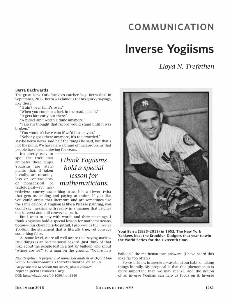
Yogi Berra (1925–2015) in 1953. The New YorkYankees beat the Brooklyn Dodgers that year to winthe World Series for the sixteenth time.

balloon!” the mathematician answers. (I have heard thisjoke far too often.)

Sowe all know in a generalway about our habit of takingthings literally. My proposal is that this phenomenon ismore important than we may realize, and the notionof an inverse Yogiism can help us focus on it. Inverse

December 2016 Notices of the AMS 1281

Yogiisms in mathematics, and in science more generally,can impede progress sometimes for generations. I willdescribe two examples from my own career and thenmention a third topic, more open-ended, that may be avery big example indeed.

Faber’s Theorem on Polynomial InterpolationThe early 1900s was an exciting time for the constructivetheory of real functions. The old idea of a function as givenby a formula hadbroadened to include arbitrarymappingsdefined pointwise, and connecting the two notions wasa matter of wide interest. In particular, mathematicianswere concerned with the problem of approximating acontinuous function 𝑓 defined on an interval such as[−1, 1] by a polynomial 𝑝. Weierstrass’s theorem of 1885had shown that arbitrarily close approximations alwaysexist, and by 1912, alternative proofs had been publishedby Picard, Lerch, Volterra, Lebesgue, Mittag-Leffler, Fejér,Landau, de la Vallée Poussin, Jackson, Sierpiński, andBernstein.

How could polynomial approximations be constructed?The simplest method would be interpolation by a degree-𝑛 polynomial in a set of 𝑛 + 1 distinct points in [−1, 1].Runge showed in 1900 that interpolants in equally spacedpoints will not generally converge to 𝑓 as 𝑛 → ∞, even foranalytic 𝑓. On the other hand, Chebyshev grids with theirpoints clustered near ±1 do much better. Yet around1912, it became clear to Bernstein, Jackson, and Faberthat no system of interpolation points could work for allfunctions. The famous result was published by Faber in1914, and here it is in his words and notation (translatedfrom [4]).Faber’s Theorem. There does not exist any set 𝐸 of in-terpolation points 𝑥(𝑛)

𝑖 in 𝑠 = (−1, 1) (𝑛 = 1, 2… ; 𝑖 =1, 2…𝑛+1) with the property that every continuous func-tion Φ(𝑥) in 𝑠 can be represented as the uniform limit ofthe degree-𝑛 polynomials taking the same values as Φ for𝑥 = 𝑥(𝑛)

𝑖 .

The proof nowadays (though not yet in 1914) makeselegant use of the uniform boundedness principle.

Faber’s theorem is true, and moreover, it is beau-tiful. Let me now explain how its influence has beenunfortunate.

The field of numerical analysis took off as soon ascomputers were invented, and the approximation offunctions was important in every area. You might thinkthat polynomial interpolation would have been one of thestandard tools from the start, and to some extent this wasthe case. However, practitioners must have often run intotrouble when they worked with polynomial interpolants— usually because of using equispaced points or unstablealgorithms, I suspect—and Faber’s theorem must havelooked like some kind of explanation of what was goingwrong. The hundreds of textbooks that soon began tobe published fell into the habit of teaching students thatinterpolation is a dangerous technique, not to be trusted.Here are some illustrations.

Isaacson andKeller,Analysis of Numerical Methods (1966),p. 275:

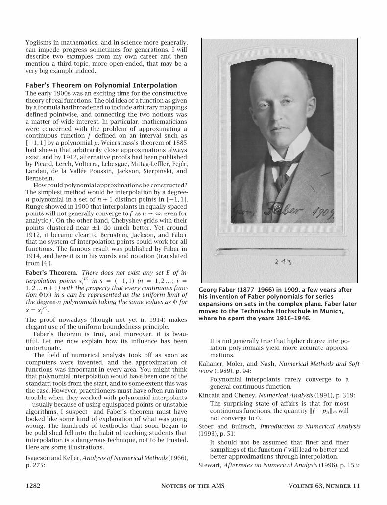
Georg Faber (1877–1966) in 1909, a few years afterhis invention of Faber polynomials for seriesexpansions on sets in the complex plane. Faber latermoved to the Technische Hochschule in Munich,where he spent the years 1916–1946.

It is not generally true that higher degree interpo-lation polynomials yield more accurate approxi-mations.

Kahaner, Moler, and Nash, Numerical Methods and Soft-ware (1989), p. 94:

Polynomial interpolants rarely converge to ageneral continuous function.

Kincaid and Cheney, Numerical Analysis (1991), p. 319:The surprising state of affairs is that for mostcontinuous functions, the quantity ‖𝑓−𝑝𝑛‖∞ willnot converge to 0.

Stoer and Bulirsch, Introduction to Numerical Analysis(1993), p. 51:

It should not be assumed that finer and finersamplings of the function 𝑓will lead to better andbetter approximations through interpolation.

Stewart, Afternotes on Numerical Analysis (1996), p. 153:

1282 Notices of the AMS Volume 63, Number 11

Unfortunately, there are functions for whichinterpolation at the Chebyshev points fails toconverge.

Gautschi, Numerical Analysis: An Introduction (1997),p. 79:

It is not possible, therefore, to conclude… thatLagrange interpolation converges uniformly on[𝑎, 𝑏] for any continuous function, not even forjudiciously selected nodes; indeed, one knowsthat it does not.

Quarteroni, Sacco, and Saleri, Numerical Mathematics(2000), p. 331:

Thus, polynomial interpolation does not allow forapproximating any continuous function….

What a load of inverse Yogiisms! Statements like these,which appear in so many of the textbooks, give entirely

Statementslike these,

which appearin so many ofthe textbooks,give entirelythe wrongimpression.

the wrong impression. In fact,polynomial interpolation inChebyshev points is a powerfuland reliable method for ap-proximation of functions. TheChebfun software system rou-tinely works with degrees in thethousands [2].

The flaw in the logic is thatFaber’s theorem says nothingif 𝑓 is smooth [7]. If 𝑓 isLipschitz continuous, that ismore than enough to guaranteeconvergence of interpolants inChebyshev points, and if it hasa 𝑘th derivative of bounded vari-ation, the error in the degree-𝑛interpolant is of size 𝑂(𝑛−𝑘). If 𝑓 is analytic, the con-vergence is at a geometric rate 𝑂(𝜌−𝑛), 𝜌 > 1. Moreover,there are methods for computing these interpolants thatare fast and numerically stable, notably the so-calledbarycentric interpolation formula.

So the idea that polynomial interpolants can’t betrusted is a myth: a myth that has drawn strength froman impeccable theorem. Make sure your functions are Lip-schitz continuous or better, as is easily done in almost anyapplication, and Faber’s theorem ceases to be applicable.In fact, polynomial interpolation in Chebyshev pointshas the same power and robustness as discrete Fourieranalysis, to which it is essentially equivalent. We musthope that the numerical analysis textbooks of futuregenerations will begin to tell students this.

Squire’s Theorem on Hydrodynamic InstabilityWe nowmove from numerical analysis to one of the oldestproblems of fluidmechanics. Consider the idealized planePoiseuille flow of a Newtonian liquid or gas in an infinitechannel between two flat plates. (The mathematics issimilar for other geometries such as a circular pipe, asinvestigated by Reynolds in 1883.) The flow is governedby the Navier-Stokes equations, and the key parameter isthe Reynolds number Re, a nondimensionalized velocity.

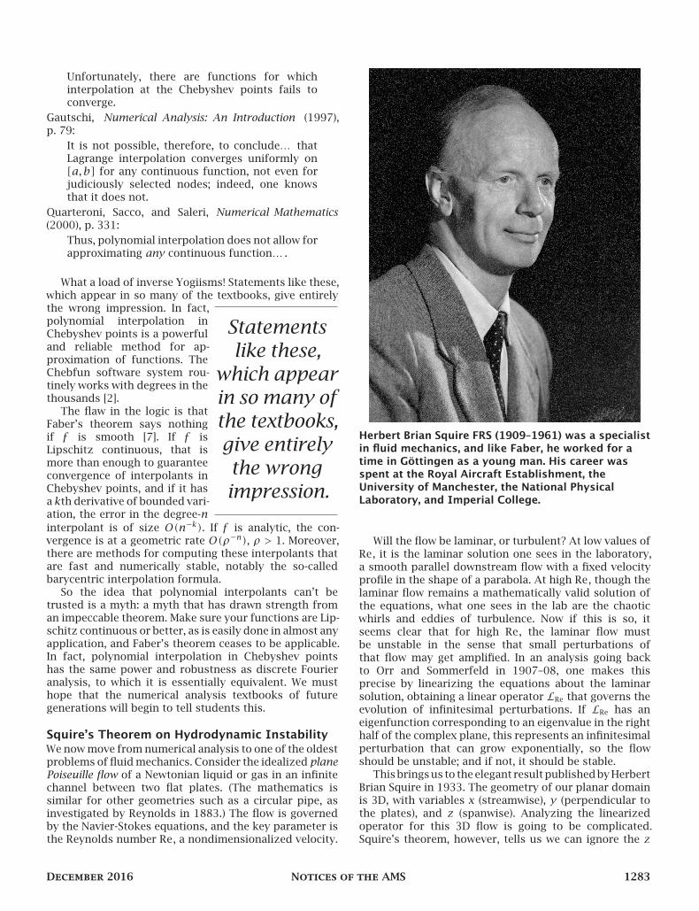
Herbert Brian Squire FRS (1909–1961) was a specialistin fluid mechanics, and like Faber, he worked for atime in Göttingen as a young man. His career wasspent at the Royal Aircraft Establishment, theUniversity of Manchester, the National PhysicalLaboratory, and Imperial College.

Will the flow be laminar, or turbulent? At low values ofRe, it is the laminar solution one sees in the laboratory,a smooth parallel downstream flow with a fixed velocityprofile in the shape of a parabola. At high Re, though thelaminar flow remains a mathematically valid solution ofthe equations, what one sees in the lab are the chaoticwhirls and eddies of turbulence. Now if this is so, itseems clear that for high Re, the laminar flow mustbe unstable in the sense that small perturbations ofthat flow may get amplified. In an analysis going backto Orr and Sommerfeld in 1907–08, one makes thisprecise by linearizing the equations about the laminarsolution, obtaining a linear operator ℒRe that governs theevolution of infinitesimal perturbations. If ℒRe has aneigenfunction corresponding to an eigenvalue in the righthalf of the complex plane, this represents an infinitesimalperturbation that can grow exponentially, so the flowshould be unstable; and if not, it should be stable.

Thisbringsus to theelegant resultpublishedbyHerbertBrian Squire in 1933. The geometry of our planar domainis 3D, with variables 𝑥 (streamwise), 𝑦 (perpendicular tothe plates), and 𝑧 (spanwise). Analyzing the linearizedoperator for this 3D flow is going to be complicated.Squire’s theorem, however, tells us we can ignore the 𝑧

December 2016 Notices of the AMS 1283

direction and just do a 2D analysis. Here is the statementfrom his original paper [6].

Squire’s Theorem. Any instability which may be presentfor three-dimensional disturbances is also present for two-dimensional disturbances at a lower value of Reynolds’number.

The influence of Squire’s theorem can be seen allacross the literature of mathematical fluid mechanics.Whenever you see an analysis involving the famousOrr–Sommerfeld equation, the authors have probablytaken a 3D flow problem and reduced it to 2D. For theplane Poiseuille configuration, the theory tells us thatthe 2D instability sets in at a critical Reynolds numberRe𝑐 ≈ 5772.22, a threshold first calculated accuratelyby Orszag. For Re < Re𝑐 we should expect stability andlaminar flow, and for Re > Re𝑐, instability and turbulence.

Here are summaries from some books.

Lin, The Theory of Hydrodynamic Stability (1967), p. 27:We shall now show, following Squire (1933), thatthe problem of three-dimensional disturbances isactually equivalent to a two-dimensional problemat a lower Reynolds number.

Tritton, Physical Fluid Dynamics (1977), p. 220:… there is a result, known as Squire’s theorem,that in linear stability theory the critical Reynoldsnumber for a two-dimensional parallel flow islowest for two dimensional perturbations. Wemay thus restrict attention to these.

Drazin and Reid, Hydrodynamic Stability (1981), p. 155:Squire’s theorem. To obtain the minimum criticalReynolds number it is sufficient to consider onlytwo-dimensional disturbances.

Friedlander and Serre, eds., Handbook of MathematicalFluid Dynamics, v. 3 (2002), p. 248:

Theorem 1.1 (Squire’s theorem, 1933). To eachunstable three-dimensional disturbance there cor-responds a more unstable two-dimensional one.

Sengupta, Instabilities of Flows and Transition to Turbu-lence (2012), p. 82:

In a two-dimensional boundary layer with realwave numbers, instability appears first for two-dimensional disturbances.

These and other sources are in agreement on a veryclear picture, and only one thing is amiss: the pictureis wrong! In the laboratory, observed structures relatedto transition to turbulence are almost invariably three-dimensional. Moreover, it is difficult to spot any changeof flow behavior at Re ≈ 5772.22. For Re < Re𝑐, manyflows are turbulent when we expect them to be laminar.For Re > Re𝑐, many flows are laminar when we expectthem to be turbulent. What is going on?

The flaw in the logic is that eigenmodal analysisapplies in the limit 𝑡 → ∞, whereas the values of 𝑡achievable in the laboratory rarely exceed 100. (Thanksto the nondimensionalization, 𝑡 is related to the length

Squire’s theoremhas told usexactly the

wrong place tolook for

hydrodynamicinstability.

of a flow apparatusrelative to its width.) Con-sequently, high-Reynoldsnumber flows normallydo not become turbu-lent in an eigenmodalfashion [8]. On the onehand, the exponentialgrowth rates of unsta-ble eigenfunctions, knownas Tollmien–Schlichtingwaves, are typically so lowthat in a laboratory setupthey struggle to amplifya perturbation by even a

factor of 2. This is why laminar flow is often observedwith Re ≫ Re𝑐. On the other hand, much faster transientamplification mechanisms are present for 3D perturba-tions, even for Re ≪ Re𝑐. The perturbations involved arenot eigenfunctions, and in principle they would die outas 𝑡 → ∞ if they started out truly infinitesimal: Squire’stheorem is, of course, literally true. But the transientgrowth of 3D perturbations is so substantial that in a realflow, small finite disturbances may quickly be raised toa level where nonlinearities kick in. In assuring us thatthe most dangerous disturbances are two-dimensional,Squire’s theorem has told us exactly the wrong place tolook for hydrodynamic instability.

P = NP?The most famous problem in computer science, whichis also one of the million-dollar Clay Millennium PrizeProblems, is the celebrated question “P = NP?” This puzzleremains unresolved half a century after it was first posedby Cook and Levin in 1971.

The precision of amathematical

formulation hasencouraged us tothink the truth issimpler than it is.

Some computa-tional problems canbe solved by fast al-gorithms, and othersonly by slow ones. Onemight expect a con-tinuum of difficulty,but the unlockingobservation was thatthere is a gulf betweenpolynomial time andexponential time algo-rithms. Inverting an

𝑛×𝑛matrix, say, can be done in𝑂(𝑛3) operations or less,so we deal routinely with matrices with dimensions inthe thousands. Finding the shortest route for a salesmanvisiting 𝑛 cities, on the other hand, requires𝐶𝑛 operationsfor some 𝐶 > 1 by all algorithms yet discovered. As𝑛 → ∞, the difference between 𝑛𝐶 and 𝐶𝑛 looks like aclean binary distinction. And there is a great class ofthousands of problems, the NP-complete problems, thathave been proved to be equivalent in the sense that all ofthem can be solved in polynomial time or none of themcan — and nobody knows which.

1284 Notices of the AMS Volume 63, Number 11

It’s an extraordinary gap in our knowledge. If I may picktwo mathematical mysteries that I hope will be resolvedbefore I die, they are the Riemann hypothesis and “P=NP?”It is so crisp, and so important!

Yet Yogi Berra seems to be looking over our shoulders.Computers are millions of times more powerful than theywere in 1971, increasing the tractable size of 𝑛 in everyproblem known to man, so one might expect that the gulfbetween P and the best known algorithms for NP, whichseemed significant already in 1971, should have openedup by now to a canyon so deep we can’t see its bottom. Yetin the event, nothing so straightforward has happened.Some NP-complete problems still defeat us. Others areeasily solvable in many instances. For example, one ofthe classic NP-complete problems is “SAT,” involvingthe satisfiability of Boolean expressions. SAT solvershave become so powerful that they are now a standardcomputational tool, solving problem instances of scales inthe thousands and evenmillions [5]. Surprisingly powerfulmethods have been developed for other NP-completeproblems too, including integer programming [1] and thetraveling salesman problem itself [3].

So is there a logical flaw in “P=NP?”, as with Faber’stheorem and Squire’s theorem? I would not go so far asto say this, but it is certainly the case that, once again, theprecision of a mathematical formulation has encouragedus to think the truth is simpler than it is. A typical NP-complete problemmeasures complexity by theworst casetime required to deliver the optimal solution. Experiencehas shown that in practice, both ends of this formulationare negotiable. For some NP-complete problems, like SAT,the worst case indeed looks exponential but in practiceit is rare for a problem instance to come close to theworst case. For others, like the “max-cut” problem, it canbe proved that even in the worst case one can solve theproblem in polynomial time, if one is willing to miss theoptimum by a few percent (for max-cut, 13 percent isenough). A field of approximation algorithms has grownup that develops algorithms of this flavor [9]. Often thesealgorithms rely on tools of continuous mathematics toapproximate problems formulated discretely. Indeed, thewhole basis of “P=NP?” is a discrete view of the world, andthe distracting sparkle of this great unsolved problemmay have delayed the recognition that often, continuousalgorithms have advantages even for discrete problems.As scientists we must always simplify the world to makesense of it; the challenge is to not get trapped by oursimplifications.

CodaWhen we say something precisely and even prove that it’strue, we open ourselves to the risk of inverse Yogiisms.Would it be better if mathematicians didn’t try so hardto be precise? Certainly not! Rigorous theorems are thepride of mathematics, which enable this unique subjectto advance from one century to the next. The point is onlythat we must always strive to examine a problem fromdifferent angles, to think widely about its context as wellas technically about its details. Or as Yogi put it,

“Sometimes you can see a lot just by looking.”

AcknowledgmentsMany people made good suggestions as I was writingthis essay. I would like particularly to acknowledgeTadashi Tokieda and David Williamson.

ReferencesBooks cited in the quotations are readily tracked down from

the information given there; I have quoted from the earliesteditions I had access to. Other references are as below.

[1] R. E. Bixby, A brief history of linear and mixed-integerprogramming computation, Documenta Mathematica (2012),107–121.

[2] Chebfun software project, www.chebfun.org.[3] W. J. Cook, The Traveling Salesman Problem,

www.math.uwaterloo.ca/tsp.[4] G. Faber, Über die interpolatorische Darstellung stetiger

Funktionen, Jber. Deutsch. Math. Verein. 23 (1914), 192–210.[5] D. E. Knuth, Satisfiability, v. 4 fascicle 6 of The Art of

Computer Programming, 2015.[6] H. B. Squire, On the stability for three-dimensional distur-

bances of viscous fluid flow between parallel walls, Proc. Roy.Soc. Lond. A 142 (1933), 621–628.

[7] L. N. Trefethen, Approximation Theory and ApproximationPractice, SIAM, 2013.

[8] L. N. Trefethen, A. E. Trefethen, S. C. Reddy, andT. A. Driscoll, Hydrodynamic stability without eigenvalues,Science 261 (1993), 578–584.

[9] D. P. Williamson and D. B. Shmoys, The Design ofApproximation Algorithms, Cambridge U. Press, 2011.

CreditsPhoto of Georg Faber is courtesy of Eberhard Karls

Universität Tübingen.Photo of Herbert Brian Squire is courtesy of The Royal

Society.Photo of Nick Trefethen is courtesy of Sara

Kerens.Photo of Yogi Berra is in the public domain.

ABOUT THE AUTHOR

Nick Trefethen FRS is professor of numerical analysis at the Uni-versity of Oxford. His college, Balliol, is the same one where Squire was an undergraduate.

Nick Trefethen Nick Trefethen

ABOUT THE AUTHOR

Nick Trefethen FRS is professor of numerical analysis at the Uni-versity of Oxford. His college, Balliol, is the same one where Squire was an undergraduate.

December 2016 Notices of the AMS 1285