2015 EUROPEAN CANSAT COMPETITION

TIPS FOR TEAMS

Written by ESA Education Office in collaboration with T-Minus Engineering

2

Table of contents

1 INTRODUCTION ........................................................................................................................................................ 5

2 THE EUROPEAN CANSAT COMPETITION: MEET THE TEAM AND DELIVERABLES .......................... 6 2.1 TEAM MEMBERS ........................................................................................................................................................ 6 2.2 DELIVERABLES .......................................................................................................................................................... 6

2.2.1 Preliminary Design Review - PDR (First report) ............................................................................................... 6 2.2.2 Critical Design Review - CDR (Second report) .................................................................................................. 7 2.2.3 Final Design Review - FDR (Third report) ........................................................................................................ 7 2.2.4 Team Presentation (Briefing) ............................................................................................................................. 7 2.2.5 Presentation of results (Debriefing) ................................................................................................................... 8 2.2.6 CanSat Final Paper – CFP (Final report).......................................................................................................... 8

2.3 TIMELINE .................................................................................................................................................................. 8

3 ANATOMY OF A SATELLITE ................................................................................................................................. 9 3.1 ATTITUDE AND ORBIT CONTROL ............................................................................................................................... 9

3.1.1 Spin stabilised satellite ..................................................................................................................................... 10 3.1.2 Dual spinner satellite ........................................................................................................................................ 10 3.1.3 Three-axis stabilized ......................................................................................................................................... 11

3.2 POWER SYSTEM ....................................................................................................................................................... 12 3.2.1 Solar Arrays ...................................................................................................................................................... 12 3.2.2 Batteries ............................................................................................................................................................ 13 3.2.3 Radioisotope Thermoelectric Generators (RTG's) ........................................................................................... 13

3.3 PROPULSION ............................................................................................................................................................ 13 3.4 TELEMETRY, TRACKING AND COMMAND ................................................................................................................ 14 3.5 DATA HANDLING ..................................................................................................................................................... 14 3.6 THERMAL CONTROL ................................................................................................................................................ 14 3.7 STRUCTURE AND MECHANISMS ............................................................................................................................... 15

4 INTRODUCTION TO SYSTEM ENGINEERING ................................................................................................ 16 4.1 PROJECT OBJECTIVES - MISSION OBJECTIVES .......................................................................................................... 16 4.2 PROJECT REQUIREMENTS ........................................................................................................................................ 16

4.2.1 CanSat General Requirements. ......................................................................................................................... 17 4.3 CANSAT MISSION REQUIREMENTS .......................................................................................................................... 18 4.4 TRADE-OFFS ............................................................................................................................................................ 20

5 MISSION DESIGN .................................................................................................................................................... 21 5.1.1 Primary mission ................................................................................................................................................ 22 5.1.2 Secondary mission ............................................................................................................................................ 22

6 INTRODUCTION TO MEASUREMENT TOOLS ................................................................................................ 24 6.1 LENGTH ................................................................................................................................................................... 24

6.1.1 Ruler ................................................................................................................................................................. 24 6.1.2 Caliper .............................................................................................................................................................. 25

6.2 ANGLES ................................................................................................................................................................... 26 6.2.1 Protractor ......................................................................................................................................................... 26 6.2.2 T-square ............................................................................................................................................................ 27

6.3 MASS ...................................................................................................................................................................... 27 6.3.1 Scale .................................................................................................................................................................. 28

6.4 ELECTRONICS: VOLTAGE, CURRENT, RESISTANCE ................................................................................................... 28 6.4.1 Multimeter......................................................................................................................................................... 29

3

7 INTRODUCTION TO ELECTRICAL CIRCUITS ............................................................................................... 30 7.1 READING OF A CIRCUIT ............................................................................................................................................ 30 7.2 COMPONENTS .......................................................................................................................................................... 31 7.3 SENSORS ................................................................................................................................................................. 33 7.4 COMMUNICATION .................................................................................................................................................... 36

8 INTRODUCTION TO SOLDERING AND CIRCUIT ASSEMBLY.................................................................... 38 8.1 SOLDERING ............................................................................................................................................................. 39

9 BATTERIES AND POWER SYSTEM .................................................................................................................... 41 9.1 BATTERY TYPES ...................................................................................................................................................... 41 9.2 ADVANTAGES AND DISADVANTAGES ...................................................................................................................... 42 9.3 CALCULATIONS WITH A BATTERY ........................................................................................................................... 42 9.4 BATTERY TIPS AND TRICKS ...................................................................................................................................... 42

10 RADIO COMMUNICATION ................................................................................................................................... 44

11 PARACHUTE DESIGN AND CONSTRUCTION ................................................................................................. 47 11.1 THE PHYSICS BEHIND THE DRAG PARACHUTE .......................................................................................................... 48 11.2 SHAPES OF DRAG PARACHUTE ................................................................................................................................. 49 11.3 LIFTING PARACHUTE ............................................................................................................................................... 50 11.4 TESTING YOUR PARACHUTE .................................................................................................................................... 51

12 INTRODUCTION TO PROGRAMMING .............................................................................................................. 52 12.1 DATA INCONSISTENCIES .......................................................................................................................................... 53

13 INTRODUCTION TO DATA ANALYSIS .............................................................................................................. 54 13.1 FROM DATA TO MEASUREMENTS: CALIBRATION ...................................................................................................... 54 13.2 RESULTS PRESENTATION ......................................................................................................................................... 56

14 PRESENTATION, REPORTS AND BLOGS ......................................................................................................... 60 14.1 BRIEFING AND DEBRIEFING PRESENTATIONS........................................................................................................... 60 14.2 REPORTS ................................................................................................................................................................. 61 14.3 TEAM BLOG ............................................................................................................................................................. 61

15 BUDGET CONSTRAINTS ....................................................................................................................................... 62

16 EXAMPLE OF CANSAT SETUP WITH THE EUROPEAN CANSAT KIT...................................................... 63

17 OTHER RESOURCES AND FURTHER INFORMATION ................................................................................. 64

4

1 INTRODUCTION

The European Space Agency (ESA) endorses and supports a range of CanSat activities across its Member States. The CanSat project, aimed at secondary school students, is mainly addressing technology, physics and programming curricular subjects. The CanSat activity provides the students with practical experience on a small-scale space project and promotes team work. A CanSat is a simulation of a real satellite, integrated within the volume and shape of a soft drink can. The challenge for the students is to fit all the major subsystems found in a satellite, such as power, sensors and a communication system, into this minimal volume. The CanSat is then launched to an altitude of a few hundred metres by a rocket or dropped from a platform or balloon and its mission begins to carry out a scientific experiment and achieve a safe landing. CanSats offer a unique opportunity for students to have a first practical experience of a real space project. They are responsible for all aspects: selecting the mission objectives, designing the CanSat, integrating the components, testing, preparing for launch and then analysing the data.

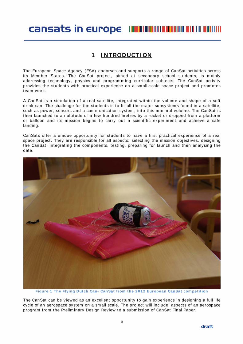
Figure 1 The Flying Dutch Can- CanSat from the 2012 European CanSat competition

The CanSat can be viewed as an excellent opportunity to gain experience in designing a full life cycle of an aerospace system on a small scale. The project will include aspects of an aerospace program from the Preliminary Design Review to a submission of CanSat Final Paper.

5

2 THE EUROPEAN CANSAT COMPETITION: MEET THE TEAM AND DELIVERABLES

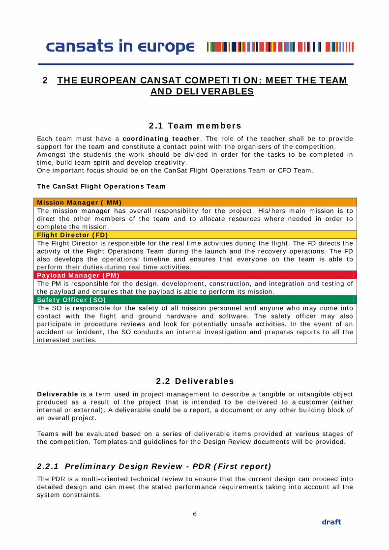
2.1 Team members Each team must have a coordinating teacher. The role of the teacher shall be to provide support for the team and constitute a contact point with the organisers of the competition. Amongst the students the work should be divided in order for the tasks to be completed in time, build team spirit and develop creativity. One important focus should be on the CanSat Flight Operations Team or CFO Team. The CanSat Flight Operations Team Mission Manager ( MM) The mission manager has overall responsibility for the project. His/hers main mission is to direct the other members of the team and to allocate resources where needed in order to complete the mission. Flight Director (FD) The Flight Director is responsible for the real time activities during the flight. The FD directs the activity of the Flight Operations Team during the launch and the recovery operations. The FD also develops the operational timeline and ensures that everyone on the team is able to perform their duties during real time activities. Payload Manager (PM) The PM is responsible for the design, development, construction, and integration and testing of the payload and ensures that the payload is able to perform its mission. Safety Officer (SO) The SO is responsible for the safety of all mission personnel and anyone who may come into contact with the flight and ground hardware and software. The safety officer may also participate in procedure reviews and look for potentially unsafe activities. In the event of an accident or incident, the SO conducts an internal investigation and prepares reports to all the interested parties.

2.2 Deliverables Deliverable is a term used in project management to describe a tangible or intangible object produced as a result of the project that is intended to be delivered to a customer (either internal or external). A deliverable could be a report, a document or any other building block of an overall project. Teams will be evaluated based on a series of deliverable items provided at various stages of the competition. Templates and guidelines for the Design Review documents will be provided.

2.2.1 Preliminary Design Review - PDR (First report) The PDR is a multi-oriented technical review to ensure that the current design can proceed into detailed design and can meet the stated performance requirements taking into account all the system constraints.

6

The CanSat PDR shall contain: • A demonstration that all the requirements stated in the guidelines for the European

CanSat Competition have been fulfilled • The stating of the secondary mission • The design specifications in order to fulfil the secondary mission • The preliminary budget • The detailed development budget • An outline of the project schedule

2.2.2 Critical Design Review - CDR (Second report) The CDR is a multi-oriented technical review to ensure that design can meet the stated performance requirements taking into account all the system constraints. The Critical Design Review evaluates the detailed design effort, determines readiness for hardware fabrication and for software coding and establishes the final configuration of the secondary mission. The CDR is an altered version of the PDR; it shall include all the discrepancies from the Preliminary Design Review and will assess the progress of technical performance measures. All major documentation and plans are reviewed. The CanSat CDR shall contain:

• The progress from the PDR • Results of requirements verification tests completed to date • Overview of mission operation • Revised budget • Revised outline of the project schedule

2.2.3 Final Design Review - FDR (Third report) The Final Design Review is the final report that should be submitted before the Launch. This report will contain all the alterations made to the CDR design and their implementation. This document should accurately record all the details of the completed CanSat prototype. The CanSat FDR shall contain:

• The progress from the CDR • Results of requirements verification tests completed to date • Overview of mission operation • Revised budget • Revised outline of the project schedule

2.2.4 Team Presentation (Briefing) The briefing presentation will take place after the Launch. Each team must present their project to the other teams and the Jury members. The briefing will contain:

• General description of mission objectives • Description of the design • Success or failure criteria

7

2.2.5 Presentation of results (Debriefing) The debriefing presentation will take place after the Launch. Each team must present the data obtained during the flight and the mission analysis. The debriefing will contain:

• General description of mission objectives • Description of the design • Graphics of the data obtained during the flight • Analysis of the data obtained • Success or failure analysis • Conclusions

2.2.6 CanSat Final Paper – CFP (Final report) The CanSat Final Paper is a document which follows the standards of a scientific paper including an abstract and a manuscript of the project.

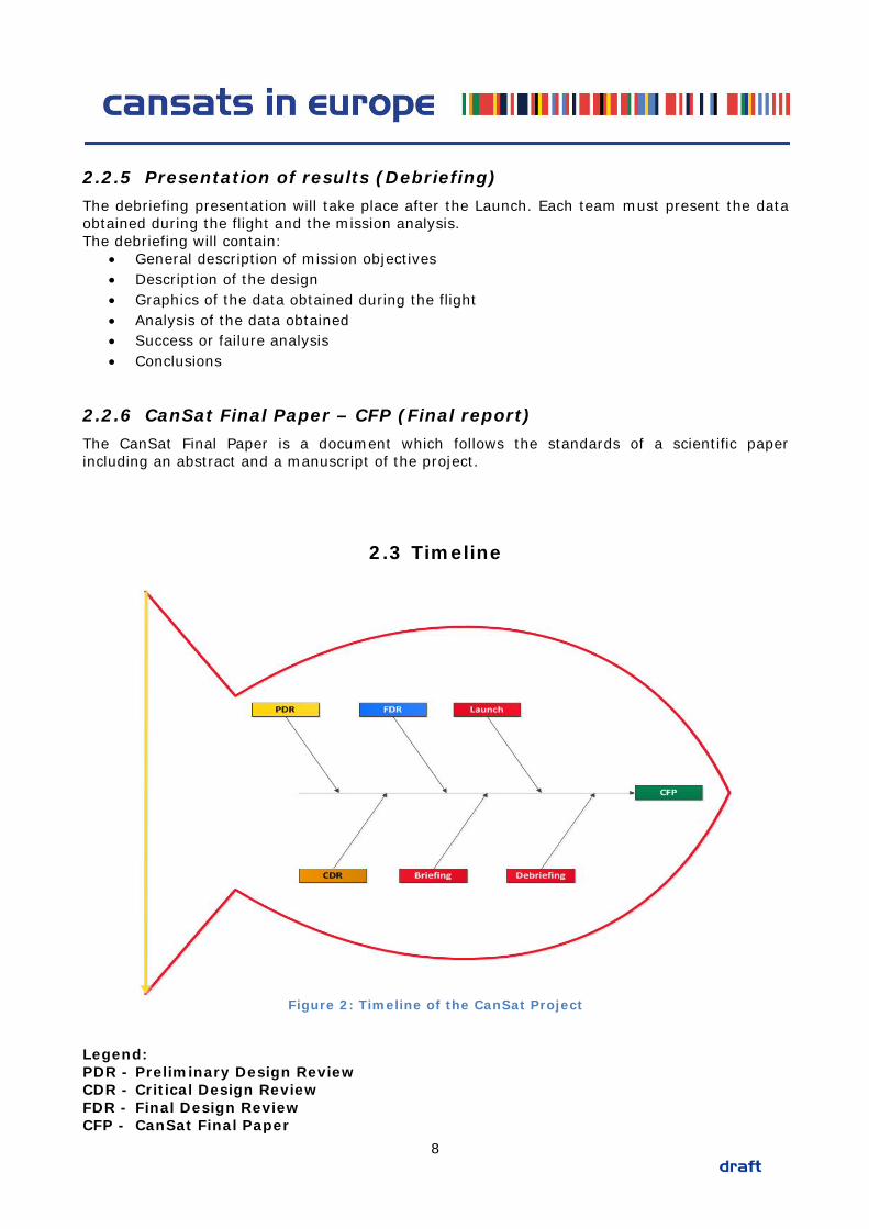
2.3 Timeline

Figure 2: Timeline of the CanSat Project

Legend: PDR - Preliminary Design Review CDR - Critical Design Review FDR - Final Design Review CFP - CanSat Final Paper

8

3 ANATOMY OF A SATELLITE

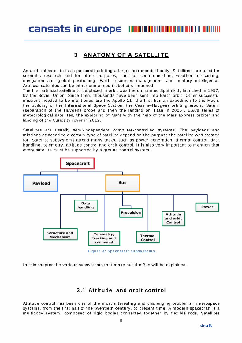
An artificial satellite is a spacecraft orbiting a larger astronomical body. Satellites are used for scientific research and for other purposes, such as communication, weather forecasting, navigation and global positioning, Earth resources management and military intelligence. Artificial satellites can be either unmanned (robotic) or manned. The first artificial satellite to be placed in orbit was the unmanned Sputnik 1, launched in 1957, by the Soviet Union. Since then, thousands have been sent into Earth orbit. Other successful missions needed to be mentioned are the Apollo 11- the first human expedition to the Moon, the building of the International Space Station, the Cassini–Huygens orbiting around Saturn (separation of the Huygens probe and then the landing on Titan in 2005), ESA’s series of meteorological satellites, the exploring of Mars with the help of the Mars Express orbiter and landing of the Curiosity rover in 2012. Satellites are usually semi-independent computer-controlled systems. The payloads and missions attached to a certain type of satellite depend on the purpose the satellite was created for. Satellite subsystems attend many tasks, such as power generation, thermal control, data handling, telemetry, attitude control and orbit control. It is also very important to mention that every satellite must be supported by a ground control system.

Figure 3: Spacecraft subsystems

In this chapter the various subsystems that make out the Bus will be explained.

3.1 Attitude and orbit control Attitude control has been one of the most interesting and challenging problems in aerospace systems, from the first half of the twentieth century, to present time. A modern spacecraft is a multibody system, composed of rigid bodies connected together by flexible rods. Satellites

9

must have a precise orbit in order for their measurements to be exact (e.g. how the camera is facing and the angle the satellite makes with the object that it is orbiting). The satellite once placed in its orbit, experiences various perturbing torques. These include gravitational forces from other bodies like solar and lunar attraction, magnetic field interaction, solar radiation pressure, etc. Due to these factors, the satellite orbit tends to drift and its orientation also changes. From a mechanical point of view and with the aim of controlling its orientation, however, it can be modelled as a single rigid body. The attitude and orbit control system maintains the satellite position and its orientation and keeps the antenna correctly pointed in the desired direction. The orbit control is performed by firing thrusters in the desired direction, by releasing a jet of gas or using spinning or gyroscopic motion systems. There are several configurations for stabilizing a satellite:

• spin stabilized • dual spinner • three-axis stabilized

3.1.1 Spin stabilised satellite The entire satellite including its antenna(s) spins. Spin-stabilized satellites are generally cylindrical in shape. The satellite's attitude becomes very stable because the satellite is acting like a gyroscope. The spinning motion can be achieved using rods with coils of wire around them through which an electric current is passed, creating thus an electromagnetic field around the wires. When the induced electromagnetic field interacts with the Earth's magnetic field, the rods begin to spin. Usually the satellite has rods in three opposing directions that achieve spin stability in all three axes (x,y,z). [abscissa, ordonate, applicate]. This design comes with a serious disadvantage, coming from the fact that if the satellite uses solar panels for power they will not face the Sun at all times and the instruments can only take measurements in one direction once every rotation.

3.1.2 Dual spinner satellite The spun/despun attitude control system works on the same principle as the spin stabilized satellite. The antenna and the other instruments of the satellite can only point towards their target once every rotation. If the antenna must be pointed toward its target at all times then a solution has been found by mounting it on a platform which is "despun" or counter-rotated. Equipment on a despun platform will point toward the same direction at all times, regardless of the spinning satellite. In the simple spinner configuration, the satellite payload and other subsystems are placed in the spinning section, while the antenna and the feed are placed in the de-spun platform. The de-spun platform is spun in a direction opposite to that of the spinning satellite body. In the dual spinner configuration, the entire payload along with the antenna and the feed is placed on the de-spun platform and the other subsystems are located on the spinning body. In both configurations, solar cells are mounted on the cylindrical body of the satellite.

10

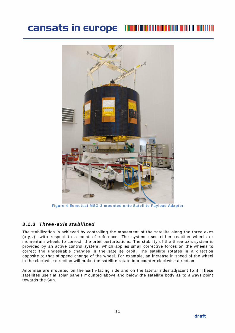
Figure 4:Eumetsat MSG-3 mounted onto Satellite Payload Adapter

3.1.3 Three-axis stabilized The stabilization is achieved by controlling the movement of the satellite along the three axes (x,y,z), with respect to a point of reference. The system uses either reaction wheels or momentum wheels to correct the orbit perturbations. The stability of the three-axis system is provided by an active control system, which applies small corrective forces on the wheels to correct the undesirable changes in the satellite orbit. The satellite rotates in a direction opposite to that of speed change of the wheel. For example, an increase in speed of the wheel in the clockwise direction will make the satellite rotate in a counter clockwise direction. Antennae are mounted on the Earth-facing side and on the lateral sides adjacent to it. These satellites use flat solar panels mounted above and below the satellite body as to always point towards the Sun.

11

3.2 Power system The electrical power system is the core of the spacecraft. In order to determine the best power budget certain constraints are taken into account such as the orbit selection, nature of the mission (e.g. how many instruments you are going to have on board), the duration of your mission, etc. The power system generates, stores, controls and distributes power within the specified voltage band to all bus and payload equipment. The protection of the power system components in case of all faults is also included.

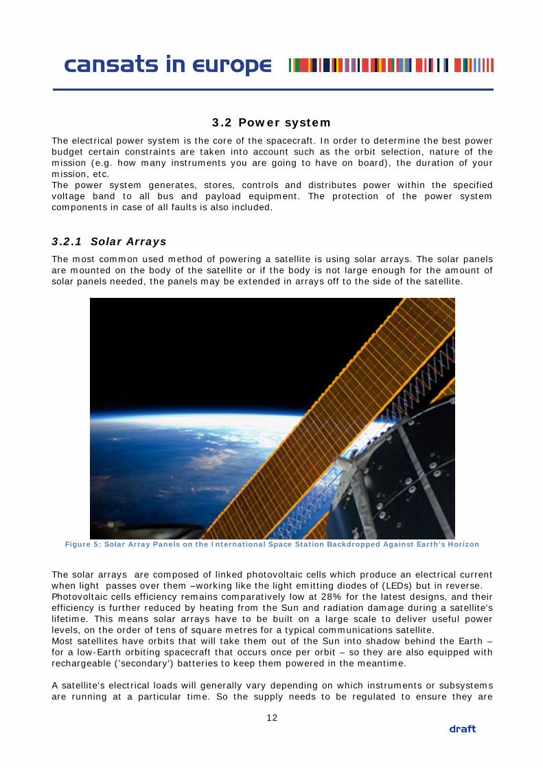
3.2.1 Solar Arrays The most common used method of powering a satellite is using solar arrays. The solar panels are mounted on the body of the satellite or if the body is not large enough for the amount of solar panels needed, the panels may be extended in arrays off to the side of the satellite.

Figure 5: Solar Array Panels on the International Space Station Backdropped Against Earth's Horizon

The solar arrays are composed of linked photovoltaic cells which produce an electrical current when light passes over them –working like the light emitting diodes of (LEDs) but in reverse. Photovoltaic cells efficiency remains comparatively low at 28% for the latest designs, and their efficiency is further reduced by heating from the Sun and radiation damage during a satellite's lifetime. This means solar arrays have to be built on a large scale to deliver useful power levels, on the order of tens of square metres for a typical communications satellite. Most satellites have orbits that will take them out of the Sun into shadow behind the Earth – for a low-Earth orbiting spacecraft that occurs once per orbit – so they are also equipped with rechargeable ('secondary') batteries to keep them powered in the meantime. A satellite's electrical loads will generally vary depending on which instruments or subsystems are running at a particular time. So the supply needs to be regulated to ensure they are

12

producing a level of power equal to that required by the satellite. The electricity is then distributed to the various elements requiring it, overseen by the power system. Solar arrays are commonly used together with a battery, which recharges when the satellite is facing the Sun and provides the satellite's power when the satellite is not. Solar arrays are used for satellites studying the Sun or the planets orbiting close to the Sun. They cannot be used easily for space exploration satellites going deep into space because they will travel too far from the Sun to receive sufficient power.

3.2.2 Batteries Batteries are commonly used as a secondary power source. They are moderately efficient and moderately expensive but very heavy so they will increase the cost for the launching of the satellite. Some batteries are rechargeable, but recharging them would require some other source of power in orbit. In a battery, electricity is produced by the transfer of electrons from one strip of metal to another, this is made possible by the fact that both metals are submerged in a solution that conducts electricity (an electrolyte). Electrons are carried over from one strip to another by particles in the solution.

3.2.3 Radioisotope Thermoelectric Generators (RTG's) Radioisotope power sources have been an important source of energy in space, used since 1961 to power satellites and unmanned space probes, because they are very efficient and durable. A radioisotope thermoelectric generator (RTG, RITEG) is an electrical generator that obtains its power from radioactive decay. The heat released by the decay of a suitable radioactive material is converted into electricity by the Seebeck effect using an array of thermocouples.

3.3 Propulsion Satellites require very little propulsion after they are launched in orbit. An orbit is a gravitationally curved path of an object around a point in space. A satellite's orbit is a balance between two forces: velocity - the speed it is travelling in a straight line - and the force of the Earth's gravitational pull on the satellite. A very important factor in the design process of a satellite is determining the orbit. Therefore, a satellite that has a very high orbit will not be able to see objects on Earth in as much detail as in lower orbits closer to the Earth's surface. Similarly, the speed of the satellite moving in the orbit, the angle over the Earth the satellite takes, the areas which the satellite can observe, and the frequency with which the satellite passes over the same portions of the Earth are all important factors to consider when choosing an orbit. The European Space Agency launches its satellites from the European Space Port in Kourou, French Guyana located approximately 500 kilometres (310 mi) north of the equator, at a latitude of 5°10'. At this latitude, the Earth's rotation gives a velocity of approximately 460 metres per second (1,000 mph; 1,700 km/h) when the launch trajectory heads eastward. The proximity to the equator also makes manoeuvring satellites for geosynchronous orbits simpler and less costly. The near-equatorial launch location provides an advantage for launches to low-inclination Earth orbits (such as geostationary) compared to launches from higher latitudes. For example, the eastward boost provided by the Earth's rotation is about 463 m/s (1,035 miles per hour) at

13

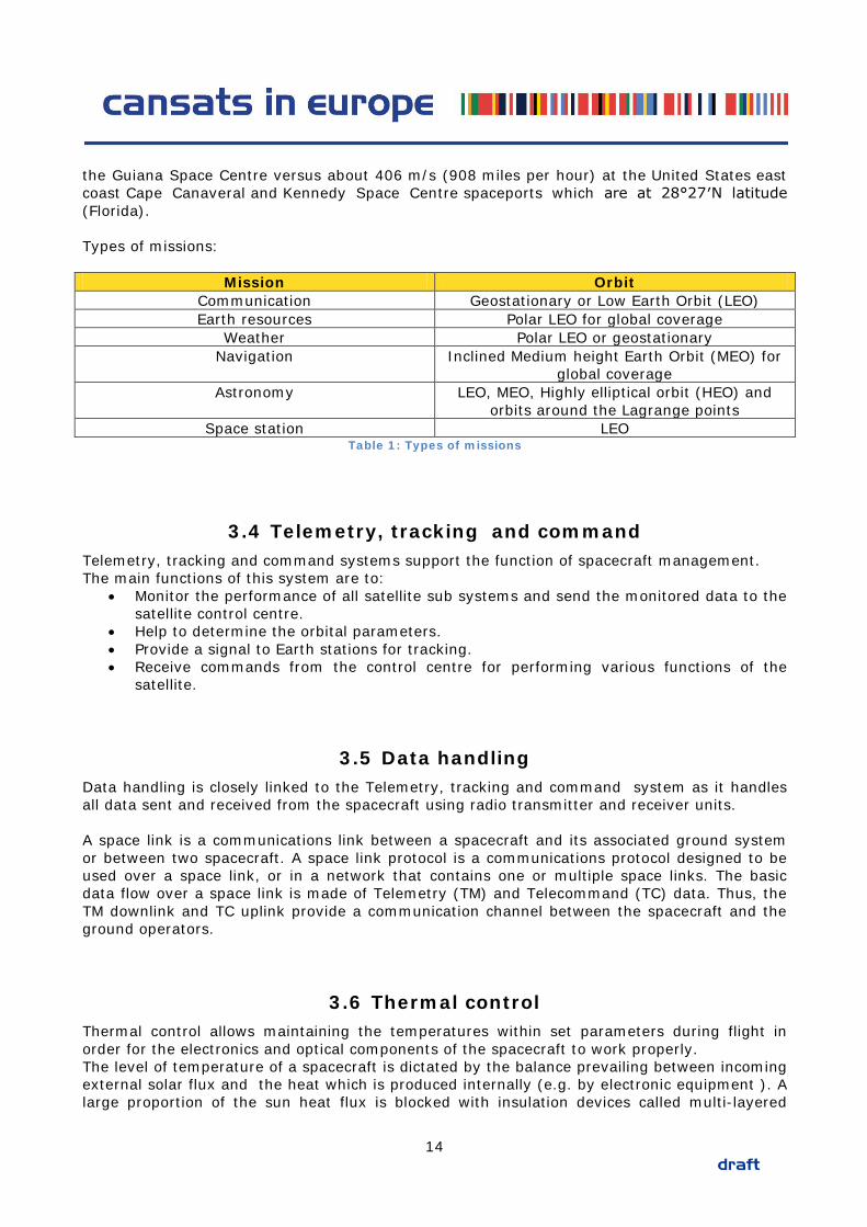
the Guiana Space Centre versus about 406 m/s (908 miles per hour) at the United States east coast Cape Canaveral and Kennedy Space Centre spaceports which are at 28°27′N latitude (Florida). Types of missions:

Mission Orbit Communication Geostationary or Low Earth Orbit (LEO) Earth resources Polar LEO for global coverage

Weather Polar LEO or geostationary Navigation Inclined Medium height Earth Orbit (MEO) for

global coverage Astronomy LEO, MEO, Highly elliptical orbit (HEO) and

orbits around the Lagrange points Space station LEO

Table 1: Types of missions

3.4 Telemetry, tracking and command Telemetry, tracking and command systems support the function of spacecraft management. The main functions of this system are to:

• Monitor the performance of all satellite sub systems and send the monitored data to the satellite control centre.

• Help to determine the orbital parameters. • Provide a signal to Earth stations for tracking. • Receive commands from the control centre for performing various functions of the

satellite.

3.5 Data handling Data handling is closely linked to the Telemetry, tracking and command system as it handles all data sent and received from the spacecraft using radio transmitter and receiver units. A space link is a communications link between a spacecraft and its associated ground system or between two spacecraft. A space link protocol is a communications protocol designed to be used over a space link, or in a network that contains one or multiple space links. The basic data flow over a space link is made of Telemetry (TM) and Telecommand (TC) data. Thus, the TM downlink and TC uplink provide a communication channel between the spacecraft and the ground operators.

3.6 Thermal control Thermal control allows maintaining the temperatures within set parameters during flight in order for the electronics and optical components of the spacecraft to work properly. The level of temperature of a spacecraft is dictated by the balance prevailing between incoming external solar flux and the heat which is produced internally (e.g. by electronic equipment ). A large proportion of the sun heat flux is blocked with insulation devices called multi-layered

14

insulation blankets (MLIs). The heat is rejected from the satellite to space (which is very cold, at a temperature of about -270 ° C) via radiators. Thermal control for space applications covers a very wide temperature range, from the cryogenic level (down to -270 ° C) to high-temperature thermal protection systems (more than 2000 ° C).

3.7 Structure and mechanisms Structures and Mechanisms involves all activities connected to the launcher and satellite structure and the moving parts associated with it. The structure must be rigid enough to support the payload, able to resist environmental factors and in the same time as light as possible. Moving mechanisms attached to the rigid structure are very crucial to mission success (e.g. motors, reaction wheels and deployment systems for folded-down antennas or solar arrays) because they can produce vibrations and distort the readings provided by the instruments.

15

4 INTRODUCTION TO SYSTEM ENGINEERING

Systems engineering is an interdisciplinary field of engineering focusing on how complex engineering projects should be designed and managed over their life cycles. Project management is the discipline of planning, organizing, securing, managing, leading, and controlling resources to achieve specific goals. A project is a temporary endeavour with a defined beginning and end (usually time-constrained, and often constrained by funding or deliverables), undertaken to meet unique goals and objectives, typically to bring about beneficial change or added value. The primary challenge of project management is to achieve all of the project goals and objectives while honouring the preconceived constraints. The primary constraints are scope, time, quality and budget. The secondary —and more ambitious— challenge is to optimize the allocation of necessary inputs and integrate them to meet pre-defined objectives. All projects begin as a concept on which you expand through progressive elaboration. Progressive elaboration is usually iterative and it simply means breaking down the ideas into steps that completely fulfil the project objectives and constraints. In spacecraft engineering the mission of the satellite determines its design.

4.1 Project objectives - Mission objectives Managing any project requires setting some clear objectives. A clear definition of the project’s objectives leads to attainability. In defining the project objectives it is recommended to use the SMART method:

Specific: Define objectives clearly and in detail. Measurable: State the measures and performance specifications used to determine

whether the objectives have been met. Aggressive: Set challenging objectives that encourage the team to think creatively. Realistic: Set objectives the project team believes it can achieve. Time sensitive: Include the date by which you are able to achieve the objectives.

The mission objectives are imposed on the system by the user of the data gathered with our satellite.

4.2 Project Requirements In the European CanSat Competition Guidelines there is a separate section about the General Project Requirements. The requirements are to be integrated fully into the design and must reflect all aspects of the project. Requirements include descriptions of system properties, specifications for how the system should work, and constraints placed upon the development process. Generally, requirements are statements of what a system should do rather than how it should do it. However, after establishing your own Mission Objectives new project requirements will ensure.

16

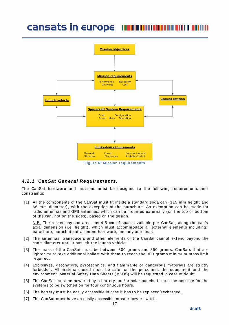
Figure 6: Mission requirements

4.2.1 CanSat General Requirements. The CanSat hardware and missions must be designed to the following requirements and constraints: [1] All the components of the CanSat must fit inside a standard soda can (115 mm height and

66 mm diameter), with the exception of the parachute. An exemption can be made for radio antennas and GPS antennas, which can be mounted externally (on the top or bottom of the can, not on the sides), based on the design.

N.B. The rocket payload area has 4.5 cm of space available per CanSat, along the can’s axial dimension (i.e. height), which must accommodate all external elements including: parachute, parachute attachment hardware, and any antennas.

[2] The antennas, transducers and other elements of the CanSat cannot extend beyond the can’s diameter until it has left the launch vehicle.

[3] The mass of the CanSat must be between 300 grams and 350 grams. CanSats that are lighter must take additional ballast with them to reach the 300 grams minimum mass limit required.

[4] Explosives, detonators, pyrotechnics, and flammable or dangerous materials are strictly forbidden. All materials used must be safe for the personnel, the equipment and the environment. Material Safety Data Sheets (MSDS) will be requested in case of doubt.

[5] The CanSat must be powered by a battery and/or solar panels. It must be possible for the systems to be switched on for four continuous hours.

[6] The battery must be easily accessible in case it has to be replaced/recharged.

[7] The CanSat must have an easily accessible master power switch. 17

[8] Inclusion of a retrieval system (beeper, radio beacon, GPS, etc.) is recommended.

[9] The CanSat should have a recovery system, such as a parachute, which is able to be reused after launch. It is recommended to use bright coloured fabric, which will facilitate recovery of the CanSat after landing.

[10] The parachute connection must be able to withstand up to 1000 N of force. The strength of the parachute must be tested, to give confidence that the system will operate nominally.

[11] For recovery reasons, a maximum flight time of 120 seconds is recommended. If attempting a directed landing then a maximum of 170 seconds flight time is recommended.

[12] A descent rate between 8 m/s and 11 m/s is recommended for recovery reasons. In case of attempting a directed landing, a lower descent rate of 6m/s is recommended.

[13] The CanSat must be able to withstand an acceleration of up to 20 g.

[14] The total budget of the final CanSat model should not exceed: 500€ for the Beginners category and 600€ for the Advanced category. Ground Stations (GS) and any related non-flying item will not be considered in the budget. More information regarding the penalties in case of exceeding the stated budget can be found in the next section.

[15] In case of sponsorship, all the items obtained should be specified in the budget with the corresponding costs on the market at that moment.

[16] The CanSat must be flight-ready upon arrival at Santa Cruz Airfield. A final technical inspection of the CanSats will be done by authorised personnel before launch.

4.3 CanSat Mission Requirements In order to establish the rest of the Mission Requirements we must take a look at our Mission Objectives and identify a way of integrating them in our design. As described in the previous chapter the spacecraft can be divided into two components the bus and the payload, below you can find a diagram of the subsystems integrated in a CanSat.

18

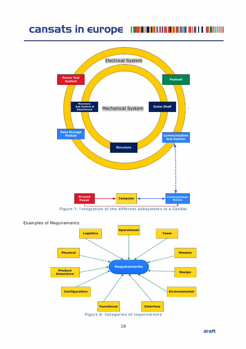
Figure 7: Integration of the different subsystems in a CanSat

Examples of Requirements:

Figure 8: Categories of requirements

19

4.4 Trade-offs The concept of a trade-off arises in a situation that involves finding the better alternative option for your design. The design is derived from the requirements and constraints imposed by the payload and means choosing one quality or aspect of something in favour of another. It often implies a decision to be made with full comprehension of both the gain and the loss of a particular choice. Major evaluation criteria for such trade-offs include:

• Cost • Satisfaction of performance requirements • Physical characteristics • Availability of technology • Flexibility to add other mission options • Reliability

Some of these criteria are considered more important than others so they can be assigned a weight out of 1.0 in order to obtain a unity sum weighting scheme. Raw scores were assigned to each alternative based on subjective criteria and rough calculations. The final weighted score is used to compare and select the best configuration used in the Critical Design Review.

Modular configuration Single board configuration Decision Criteria Weight Raw Score Weighted

Score Raw Score Weighted

Score Mounting Area 0.3 1 0.3 0.25 0.075 Ease of Integration 0.15 0.75 0.1125 1 0.15 Complexity 0.05 0.25 0.0125 1 0.05 Fault Tolerance 0.1 1 0.1 0 0 Flexibility 0.2 0 0 1 0.2 Ease of troubleshooting

0.1 1 0.1 0.25 0.025

Structural Mass 0.05 0.75 0.0375 0.25 0.0125 Cost 0.05 0.25 0.0125 1 0.05 1 0.675 0.562

Table 2: Example of a trade-off analysis

The solution in this case appears to be a Modular configuration, mainly due to the increased surface area for mounting electronic components, the ability to easily replace faulty boards in case of errors and the ability to integrate a modular assembly method in the CanSat kit training module.

20

5 MISSION DESIGN

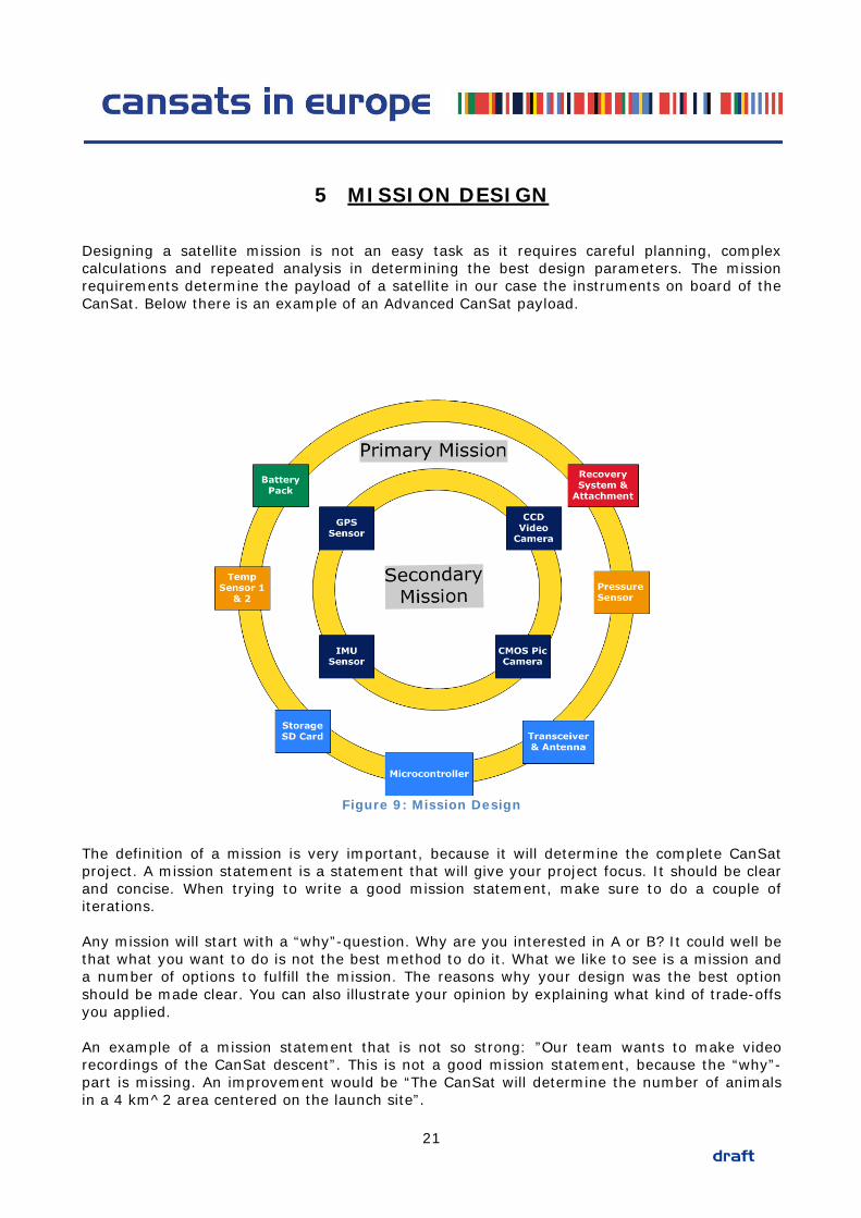
Designing a satellite mission is not an easy task as it requires careful planning, complex calculations and repeated analysis in determining the best design parameters. The mission requirements determine the payload of a satellite in our case the instruments on board of the CanSat. Below there is an example of an Advanced CanSat payload.

Figure 9: Mission Design

The definition of a mission is very important, because it will determine the complete CanSat project. A mission statement is a statement that will give your project focus. It should be clear and concise. When trying to write a good mission statement, make sure to do a couple of iterations. Any mission will start with a “why”-question. Why are you interested in A or B? It could well be that what you want to do is not the best method to do it. What we like to see is a mission and a number of options to fulfill the mission. The reasons why your design was the best option should be made clear. You can also illustrate your opinion by explaining what kind of trade-offs you applied. An example of a mission statement that is not so strong: ”Our team wants to make video recordings of the CanSat descent”. This is not a good mission statement, because the “why”-part is missing. An improvement would be “The CanSat will determine the number of animals in a 4 km^2 area centered on the launch site”.

21

In a nutshell, the mission statement is an answer to the question “what does our CanSat team want to achieve and why?” Now perhaps it is easy to think of all kind of things that one can do with a CanSat but the “and why?” part of the question is fundamental.

5.1.1 Primary mission The team must build a CanSat and program it to accomplish the compulsory primary mission, as follows: After release and during descent, the CanSat shall measure the following parameters and transmit the data as telemetry once every second to the ground station:

• Air temperature • Air pressure

It must be possible for the team to analyse the data obtained (for example, make a calculation of altitude) and display it in graphs (for example, altitude vs. time and temperature vs. altitude). For the primary mission, the reason why pressure and temperature are measured is because we can determine the altitude from that. So the primary mission would be to determine the altitude of the CanSat with the use of the temperature and pressure sensor. Notice that the organization could require other methods of determining the altitude of the CanSat in the future. Therefore, a team must be able to explain and justify why they made certain decisions.

5.1.2 Secondary mission The secondary mission for the CanSat must be selected by the team. It can be based on other satellite missions, a perceived need for scientific data for a specific project, a technology demonstration for a student-designed component, or any other mission that would fit the CanSat’s capabilities. Some examples of missions are listed below, but teams are free to design a mission of their choice, as long as it can be demonstrated to have some scientific, technological or innovative value. Teams should also keep in mind the limitations of the CanSat mission profile, and focus on the feasibility (both technical and administrative) of their chosen mission. Some example secondary missions:

1. Advanced telemetry After release and during descent, the CanSat measures and transmits additional telemetry to that required for the primary mission, for example:

• Acceleration • GPS location • Radiation levels

2. Telecommand

The main purpose of a telecommand mission is to transmit data during descent, also commands are sent from the ground to the CanSat to perform an action, such as switching a sensor on and off, changing the frequency of measurements, etc. CanSats in this category do not use a steering system.

3. Targeted landing

22

The CanSat navigates autonomously with a control mechanism such as a ram-air parachute. The objective is for the CanSat to land as close as possible to a fixed target point on the ground after it has been released from the rocket. This mission is an advanced telemetry/telecommand mission - navigation data is exchanged between the CanSat and a ground station throughout the descent.

4. Comeback CanSat

For this mission, an alternative safe landing system for the CanSat would be deployed, such as a bespoke parachute or airbag. The main task of these is to land in a controlled manner as close as possible to a target marked by GPS coordinates. A Comeback CanSat always carries a steering system that allows it to manoeuvre, to orient and to move towards the target. Normally such a mechanism is actuated by one or more actuator(s) controlled by the microprocessor so that the servomotor rotates to one side or the other and so rotates the CanSat.

5. Planetary probe

The CanSat simulates an exploration flight to a new planet, taking measurements on the ground after landing. Teams should define their exploration mission and identify the parameters necessary to accomplish it (e.g. pressure, temperature, samples of the terrain, humidity, etc.).

23

6 INTRODUCTION TO MEASUREMENT TOOLS

During the production of your CanSat, you will very likely need to measure certain quantities: the diameter of your parachute, the mass of your CanSat, or maybe its battery voltage. To do this, you will need the proper tools. Most of them, such as the ruler or the scale, you are probably familiar with. Other tools, such as the caliper, may be new to you. This chapter will describe some of the tools that you will most likely want to use. Also, the correct usage of them is explained. The chapter is divided into four sections, in each of which a certain measurable quantity, such as length or mass, is treated.

6.1 Length The first and probably most important quantity that is measured is the size of objects. This can be the height of a CanSat, or the diameter of a thread for example. The quantity we are measuring in these cases is length, defined as the distance between two known points. Length can be defined in many units. These units are roughly defined in two systems: the imperial system and the metric system. The imperial system is the most common system used in the US and the UK. The metric system is mainly used in Europe. The units in which a length is most conveniently expressed depends on the actual size that is measured. The height of the CanSat is probably expressed in millimeters (mm), centimeters (cm) or inches (in), and the distance from your house to your school is most likely expressed in kilometers (km) or miles (mi). For the translation between one unit to the other, linear translation rules are defined. These express how many of one unit add up to another unit. For example, 100 centimeters make one meter, and 1000 meters make one kilometer. The other way around also works: one centimeter is 1/100th of a meter, which is 1/1000th of a kilometer. In a formula, this can be expressed as: 6-1 [ ] [ ]m 1000 kmLength Length= ×

Also the conversion from imperial to metric system is done via linear relations:

6-2 [ ] [ ][ ] [ ]mm 25.4 in

mi 1.609 km

Length Length

Length Length

= ×

= ×

Most of the conversion factors from one unit to the other can be found on the internet or in your science book. Many tools exist to measure length. The type of tool used depends mainly on the size of the measured object and its shape.

6.1.1 Ruler The ruler is the length measuring tool that everybody knows. It consists of a straight piece of material, with a series of tick marks at equal distance from each other, which forms the scale of the ruler. It is used for measuring linear lengths, or lengths of objects with a straight edge. Typical dimensions range from 10 cm to one meter. Measuring with a ruler is easy: the first tick mark, typically the zero-mark, is kept next to the first measurement point and the value of the tick mark at the second measurement point is read from the scale. The accuracy of the ruler is a figure that expresses the measurement error that is made with it. This figure depends on the spacing of the tick marks. If the spacing is for example 1 mm, and one reads a value of

24

59 mm between the measurement points, it means that the distance between the points may be anywhere between 58.5 and 59.5 mm. This means that the accuracy of the measurement is plus or minus 0.5 mm. This is usually expressed as: 6-3 [ ]59 0.5 mmL = ±

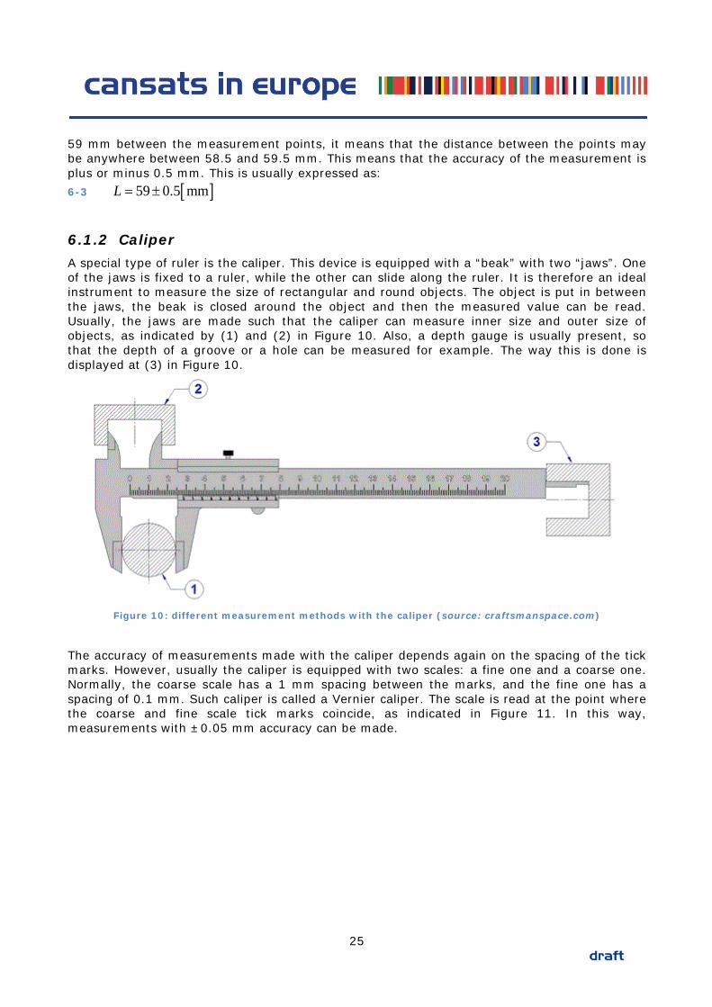
6.1.2 Caliper A special type of ruler is the caliper. This device is equipped with a “beak” with two “jaws”. One of the jaws is fixed to a ruler, while the other can slide along the ruler. It is therefore an ideal instrument to measure the size of rectangular and round objects. The object is put in between the jaws, the beak is closed around the object and then the measured value can be read. Usually, the jaws are made such that the caliper can measure inner size and outer size of objects, as indicated by (1) and (2) in Figure 10. Also, a depth gauge is usually present, so that the depth of a groove or a hole can be measured for example. The way this is done is displayed at (3) in Figure 10.

Figure 10: different measurement methods with the caliper (source: craftsmanspace.com)

The accuracy of measurements made with the caliper depends again on the spacing of the tick marks. However, usually the caliper is equipped with two scales: a fine one and a coarse one. Normally, the coarse scale has a 1 mm spacing between the marks, and the fine one has a spacing of 0.1 mm. Such caliper is called a Vernier caliper. The scale is read at the point where the coarse and fine scale tick marks coincide, as indicated in Figure 11. In this way, measurements with ±0.05 mm accuracy can be made.

25

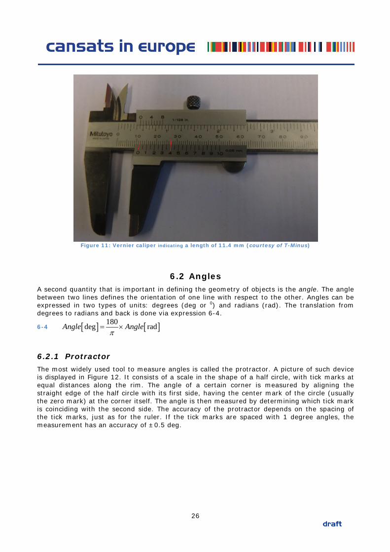
Figure 11: Vernier caliper indicating a length of 11.4 mm (courtesy of T-Minus)

6.2 Angles A second quantity that is important in defining the geometry of objects is the angle. The angle between two lines defines the orientation of one line with respect to the other. Angles can be expressed in two types of units: degrees (deg or 0) and radians (rad). The translation from degrees to radians and back is done via expression 6-4.

6-4 [ ] [ ]180deg radAngle Angleπ

= ×

6.2.1 Protractor The most widely used tool to measure angles is called the protractor. A picture of such device is displayed in Figure 12. It consists of a scale in the shape of a half circle, with tick marks at equal distances along the rim. The angle of a certain corner is measured by aligning the straight edge of the half circle with its first side, having the center mark of the circle (usually the zero mark) at the corner itself. The angle is then measured by determining which tick mark is coinciding with the second side. The accuracy of the protractor depends on the spacing of the tick marks, just as for the ruler. If the tick marks are spaced with 1 degree angles, the measurement has an accuracy of ±0.5 deg.

26

Figure 12: schematic representation of a protractor (source: math8geometry.wikispaces.com)

6.2.2 T-square A tool that is frequently used to draw corners with a defined angle is the T-square. This device is composed of two parts: the block and the ruler. The angle between the ruler and the block may be fixed at any angle between 0 and 90 deg. For drawing the corner, the ruler is fixed at the desired angle and the block is placed in alignment with the first side of the corner. The base of the ruler is positioned at the place where the corner is to be drawn. The corner can then be drawn by following the edge of the ruler with a drawing tool, for example a pencil.

Figure 13: A T-square (source: mathasteward.com)

6.3 Mass The quantities that define the shape and size of an object had been discussed. However, there is one more property of the CanSat that is important to know: its mass. Determining the mass

27

of the CanSat is necessary in order to size the parachute, and to verify if the design meets the requirements. Just like the quantity length, the mass can be expressed in metric and imperial units. Metric units are for example the kilogram (kg) or the gram (g), while the mass in imperial units is normally expressed in pounds (lb). The conversion from kilogram to pounds is done by: 6-5 [ ] [ ]kg 2.205 lbMass Mass= ×

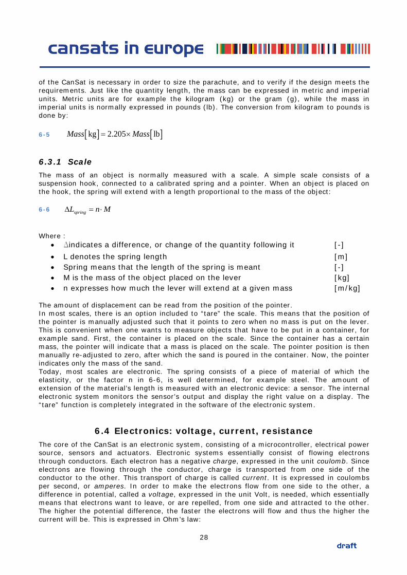
6.3.1 Scale The mass of an object is normally measured with a scale. A simple scale consists of a suspension hook, connected to a calibrated spring and a pointer. When an object is placed on the hook, the spring will extend with a length proportional to the mass of the object: 6-6 springL n M∆ = ⋅

Where :

• ∆indicates a difference, or change of the quantity following it [-] • L denotes the spring length [m] • Spring means that the length of the spring is meant [-] • M is the mass of the object placed on the lever [kg] • n expresses how much the lever will extend at a given mass [m/kg]

The amount of displacement can be read from the position of the pointer. In most scales, there is an option included to “tare” the scale. This means that the position of the pointer is manually adjusted such that it points to zero when no mass is put on the lever. This is convenient when one wants to measure objects that have to be put in a container, for example sand. First, the container is placed on the scale. Since the container has a certain mass, the pointer will indicate that a mass is placed on the scale. The pointer position is then manually re-adjusted to zero, after which the sand is poured in the container. Now, the pointer indicates only the mass of the sand. Today, most scales are electronic. The spring consists of a piece of material of which the elasticity, or the factor n in 6-6, is well determined, for example steel. The amount of extension of the material’s length is measured with an electronic device: a sensor. The internal electronic system monitors the sensor’s output and display the right value on a display. The “tare” function is completely integrated in the software of the electronic system.

6.4 Electronics: voltage, current, resistance The core of the CanSat is an electronic system, consisting of a microcontroller, electrical power source, sensors and actuators. Electronic systems essentially consist of flowing electrons through conductors. Each electron has a negative charge, expressed in the unit coulomb. Since electrons are flowing through the conductor, charge is transported from one side of the conductor to the other. This transport of charge is called current. It is expressed in coulombs per second, or amperes. In order to make the electrons flow from one side to the other, a difference in potential, called a voltage, expressed in the unit Volt, is needed, which essentially means that electrons want to leave, or are repelled, from one side and attracted to the other. The higher the potential difference, the faster the electrons will flow and thus the higher the current will be. This is expressed in Ohm’s law:

28

6-7 UIR

=

where: • I is the current through the conductor [Ampere, A] • U is the voltage over the conductor [Volt, V] • R is the resistance of the conductor [Ohm, Ω]

The resistance is essentially a figure that expresses how hard it is for electrons to flow through the conductor. A high resistance means that a high potential is needed in order to achieve a certain current. The resistance of a conductor depends amongst others on the material that the conductor is made of, the size of the conductor (length, cross-sectional area) and the temperature.

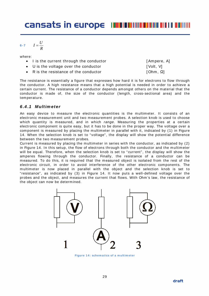
6.4.1 Multimeter An easy device to measure the electronic quantities is the multimeter. It consists of an electronic measurement unit and two measurement probes. A selection knob is used to choose which quantity is measured, and in which range. Measuring the properties at a certain electronic component is quite easy, but it has to be done in the proper way. The voltage over a component is measured by placing the multimeter in parallel with it, indicated by (1) in Figure 14. When the selection knob is set to “voltage”, the display will show the potential difference between the two measurement probes. Current is measured by placing the multimeter in series with the conductor, as indicated by (2) in Figure 14. In this setup, the flow of electrons through both the conductor and the multimeter will be equal. Therefore, when the selection knob is set to “current”, the display will show the amperes flowing through the conductor. Finally, the resistance of a conductor can be measured. To do this, it is required that the measured object is isolated from the rest of the electronic circuit, in order to avoid interference of the other electronic components. The multimeter is now placed in parallel with the object and the selection knob is set to “resistance”, as indicated by (3) in Figure 14. It now puts a well-defined voltage over the probes and the object, and measures the current that flows. With Ohm’s law, the resistance of the object can now be determined.

Figure 14: schematics of a multimeter

29

7 INTRODUCTION TO ELECTRICAL CIRCUITS

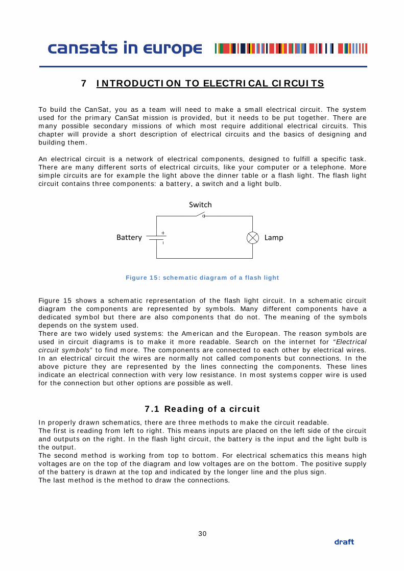
To build the CanSat, you as a team will need to make a small electrical circuit. The system used for the primary CanSat mission is provided, but it needs to be put together. There are many possible secondary missions of which most require additional electrical circuits. This chapter will provide a short description of electrical circuits and the basics of designing and building them. An electrical circuit is a network of electrical components, designed to fulfill a specific task. There are many different sorts of electrical circuits, like your computer or a telephone. More simple circuits are for example the light above the dinner table or a flash light. The flash light circuit contains three components: a battery, a switch and a light bulb.

Battery

Switch

Lamp

Figure 15: schematic diagram of a flash light

Figure 15 shows a schematic representation of the flash light circuit. In a schematic circuit diagram the components are represented by symbols. Many different components have a dedicated symbol but there are also components that do not. The meaning of the symbols depends on the system used. There are two widely used systems: the American and the European. The reason symbols are used in circuit diagrams is to make it more readable. Search on the internet for “Electrical circuit symbols” to find more. The components are connected to each other by electrical wires. In an electrical circuit the wires are normally not called components but connections. In the above picture they are represented by the lines connecting the components. These lines indicate an electrical connection with very low resistance. In most systems copper wire is used for the connection but other options are possible as well.

7.1 Reading of a circuit In properly drawn schematics, there are three methods to make the circuit readable. The first is reading from left to right. This means inputs are placed on the left side of the circuit and outputs on the right. In the flash light circuit, the battery is the input and the light bulb is the output. The second method is working from top to bottom. For electrical schematics this means high voltages are on the top of the diagram and low voltages are on the bottom. The positive supply of the battery is drawn at the top and indicated by the longer line and the plus sign. The last method is the method to draw the connections.

30

Not connectedjunction

Connectedjunction

Label

Use of labels

Use of labels

Label

Label

Label

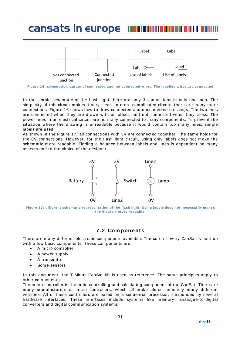
Figure 16: schematic diagram of connected and not connected wires. The labelled wires are connected

In the simple schematic of the flash light there are only 3 connections in only one loop. The simplicity of this circuit makes it very clear. In more complicated circuits there are many more connections. Figure 16 shows how to draw connected and unconnected crossings. The two lines are connected when they are drawn with an offset, and not connected when they cross. The power lines in an electrical circuit are normally connected to many components. To prevent the situation where the drawing is unreadable because it would contain too many lines, simple labels are used. As shown in the Figure 17, all connections with 3V are connected together. The same holds for the 0V connections. However, for the flash light circuit, using only labels does not make the schematic more readable. Finding a balance between labels and lines is dependent on many aspects and to the choice of the designer.

Battery Switch Lamp

3V 3V

Line2

Line2

0V 0V

Figure 17: different schematic representation of the flash light. Using labels does not necessarily makes the diagram more readable.

7.2 Components There are many different electronic components available. The core of every CanSat is built up with a few basic components. These components are:

• A micro controller • A power supply • A transmitter • Some sensors

In this document, the T-Minus CanSat kit is used as reference. The same principles apply to other components. The micro controller is the main controlling and calculating component of the CanSat. There are many manufacturers of micro controllers, which all make almost infinitely many different versions. All of these controllers are based on a sequential processor, surrounded by several hardware interfaces. These interfaces include systems like memory, analogue-to-digital converters and digital communication systems.

31

PB6 (PCINT6/XTAL1/TOSC1)5PB7 (PCINT7/XTAL2/TOSC2)6

PD0 (RXD/PCINT16) 26PD1 (TXD/PCINT17) 27PD2 (INT0/PCINT18) 28

PD3 (PCINT19/OC2B/INT1) 1PD4 (PCINT20/XCK/T0) 2

PD5 (PCINT21/OC0B/T1) 7PD6 (PCINT22/OC0A/AIN0) 8

PD7 (PCINT23/AIN1) 9PC0 (ADC0/PCINT8)19PC1 (ADC1/PCINT9)20PC2 (ADC2/PCINT10)21PC3 (ADC3/PCINT11)22PC4 (ADC4/SDA/PCINT12)23PC5 (ADC5/SCL/PCINT13)24PC6 (RESET/PCINT14)25

PB0 (PCINT0/CLKO/ICP1)10PB1 (PCINT1/OC1A)11PB2 (PCINT2/SS/OC1B)12PB3 (PCINT3/OC2A/MOSI)13PB4 (PCINT4/MISO)14PB5 (SCK/PCINT5)15

U5A

ATmega88PA

VCC3 GND 4AVCC16

Thermal Pad 29AREF17 GND 18

U5B

ATmega88PA

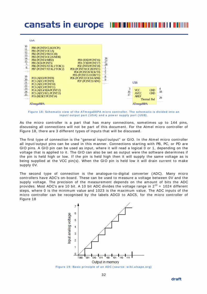
Figure 18: Schematic view of the ATmega88PA micro controller. The schematic is divided into an

input/output part (U5A) and a power supply part (U5B).

As the micro controller is a part that has many connections, sometimes up to 144 pins, discussing all connections will not be part of this document. For the Atmel micro controller of Figure 18, there are 3 different types of inputs that will be discussed. The first type of connection is the “general input/output” or GIO. In the Atmel micro controller all input/output pins can be used in this manner. Connections starting with PB, PC, or PD are GIO pins. A GIO pin can be used as input, where it will read a logical 0 or 1, depending on the voltage that is applied to it. The GIO can also be set as output were the software determines if the pin is held high or low. If the pin is held high then it will supply the same voltage as is being supplied at the VCC pin(s). When the GIO pin is held low it will drain current to make supply 0V. The second type of connection is the analogue-to-digital converter (ADC). Many micro controllers have ADC’s on-board. These can be used to measure a voltage between 0V and the supply voltage. The precision of the measurement depends on the amount of bits the ADC provides. Most ADC’s are 10 bit. A 10 bit ADC divides the voltage range in 210 = 1024 different steps, where 0 is the minimum value and 1023 is the maximum value. The ADC inputs of the micro controller can be recognised by the labels ADC0 to ADC5, for the micro controller of Figure 18

Figure 19: Basic principle of an ADC (source: wiki.ulcape.org)

32

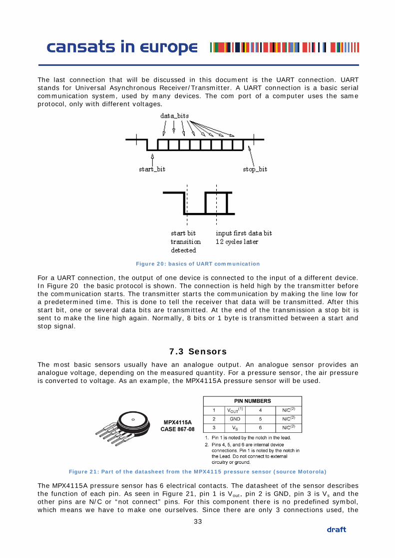
The last connection that will be discussed in this document is the UART connection. UART stands for Universal Asynchronous Receiver/Transmitter. A UART connection is a basic serial communication system, used by many devices. The com port of a computer uses the same protocol, only with different voltages.

Figure 20: basics of UART communication

For a UART connection, the output of one device is connected to the input of a different device. In Figure 20 the basic protocol is shown. The connection is held high by the transmitter before the communication starts. The transmitter starts the communication by making the line low for a predetermined time. This is done to tell the receiver that data will be transmitted. After this start bit, one or several data bits are transmitted. At the end of the transmission a stop bit is sent to make the line high again. Normally, 8 bits or 1 byte is transmitted between a start and stop signal.

7.3 Sensors The most basic sensors usually have an analogue output. An analogue sensor provides an analogue voltage, depending on the measured quantity. For a pressure sensor, the air pressure is converted to voltage. As an example, the MPX4115A pressure sensor will be used.

Figure 21: Part of the datasheet from the MPX4115 pressure sensor (source Motorola)

The MPX4115A pressure sensor has 6 electrical contacts. The datasheet of the sensor describes the function of each pin. As seen in Figure 21, pin 1 is Vout, pin 2 is GND, pin 3 is Vs and the other pins are N/C or “not connect” pins. For this component there is no predefined symbol, which means we have to make one ourselves. Since there are only 3 connections used, the

33

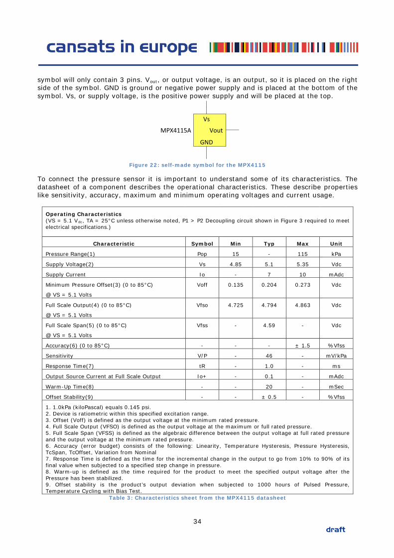
symbol will only contain 3 pins. Vout, or output voltage, is an output, so it is placed on the right side of the symbol. GND is ground or negative power supply and is placed at the bottom of the symbol. Vs, or supply voltage, is the positive power supply and will be placed at the top.

Vs

GND

VoutMPX4115A

Figure 22: self-made symbol for the MPX4115

To connect the pressure sensor it is important to understand some of its characteristics. The datasheet of a component describes the operational characteristics. These describe properties like sensitivity, accuracy, maximum and minimum operating voltages and current usage.

Operating Characteristics (VS = 5.1 Vdc, TA = 25°C unless otherwise noted, P1 > P2 Decoupling circuit shown in Figure 3 required to meet

electrical specifications.)

Characteristic Symbol Min Typ Max Unit

Pressure Range(1) Pop 15 - 115 kPa

Supply Voltage(2) Vs 4.85 5.1 5.35 Vdc

Supply Current Io - 7 10 mAdc

Minimum Pressure Offset(3) (0 to 85°C) Voff 0.135 0.204 0.273 Vdc

@ VS = 5.1 Volts

Full Scale Output(4) (0 to 85°C) Vfso 4.725 4.794 4.863 Vdc

@ VS = 5.1 Volts

Full Scale Span(5) (0 to 85°C) Vfss - 4.59 - Vdc

@ VS = 5.1 Volts

Accuracy(6) (0 to 85°C) - - - ± 1.5 %Vfss

Sensitivity V/P - 46 - mV/kPa

Response Time(7) tR - 1.0 - ms

Output Source Current at Full Scale Output Io+ - 0.1 - mAdc

Warm-Up Time(8) - - 20 - mSec

Offset Stability(9) - - ± 0.5 - %Vfss

1. 1.0kPa (kiloPascal) equals 0.145 psi. 2. Device is ratiometric within this specified excitation range.

3. Offset (Voff) is defined as the output voltage at the minimum rated pressure. 4. Full Scale Output (VFSO) is defined as the output voltage at the maximum or full rated pressure.

5. Full Scale Span (VFSS) is defined as the algebraic difference between the output voltage at full rated pressure and the output voltage at the minimum rated pressure. 6. Accuracy (error budget) consists of the following: Linearity, Temperature Hysteresis, Pressure Hysteresis, TcSpan, TcOffset, Variation from Nominal 7. Response Time is defined as the time for the incremental change in the output to go from 10% to 90% of its final value when subjected to a specified step change in pressure. 8. Warm-up is defined as the time required for the product to meet the specified output voltage after the Pressure has been stabilized. 9. Offset stability is the product’s output deviation when subjected to 1000 hours of Pulsed Pressure, Temperature Cycling with Bias Test.

Table 3: Characteristics sheet from the MPX4115 datasheet

34

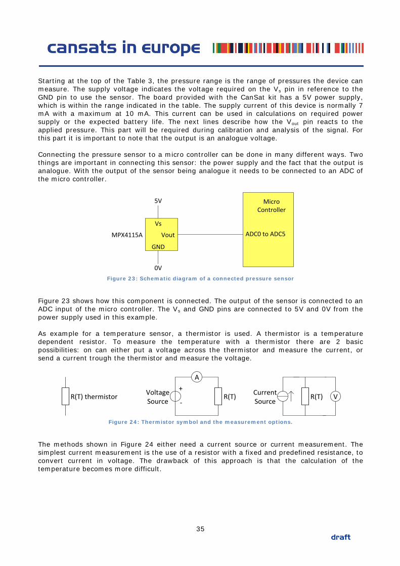
Starting at the top of the Table 3, the pressure range is the range of pressures the device can measure. The supply voltage indicates the voltage required on the Vs pin in reference to the GND pin to use the sensor. The board provided with the CanSat kit has a 5V power supply, which is within the range indicated in the table. The supply current of this device is normally 7 mA with a maximum at 10 mA. This current can be used in calculations on required power supply or the expected battery life. The next lines describe how the Vout pin reacts to the applied pressure. This part will be required during calibration and analysis of the signal. For this part it is important to note that the output is an analogue voltage. Connecting the pressure sensor to a micro controller can be done in many different ways. Two things are important in connecting this sensor: the power supply and the fact that the output is analogue. With the output of the sensor being analogue it needs to be connected to an ADC of the micro controller.

Vs

GND

VoutMPX4115A

Micro Controller

ADC0 to ADC5

5V

0V

Figure 23: Schematic diagram of a connected pressure sensor

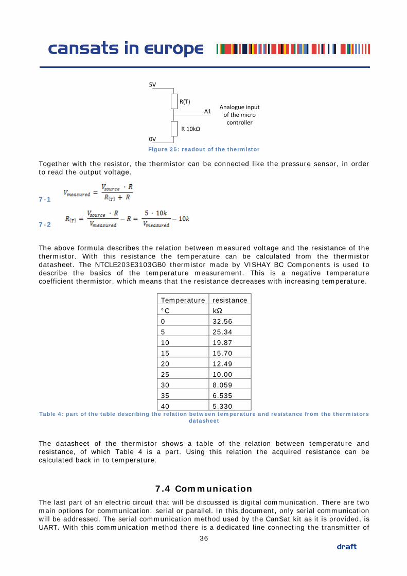
Figure 23 shows how this component is connected. The output of the sensor is connected to an ADC input of the micro controller. The Vs and GND pins are connected to 5V and 0V from the power supply used in this example. As example for a temperature sensor, a thermistor is used. A thermistor is a temperature dependent resistor. To measure the temperature with a thermistor there are 2 basic possibilities: on can either put a voltage across the thermistor and measure the current, or send a current trough the thermistor and measure the voltage.

R(T) thermistor R(T)

A+

-VoltageSource

R(T)CurrentSource

V

Figure 24: Thermistor symbol and the measurement options.

The methods shown in Figure 24 either need a current source or current measurement. The simplest current measurement is the use of a resistor with a fixed and predefined resistance, to convert current in voltage. The drawback of this approach is that the calculation of the temperature becomes more difficult.

35

R(T)

R 10kΩ

5V

0V

Analogue input of the micro

controller

A1

Figure 25: readout of the thermistor

Together with the resistor, the thermistor can be connected like the pressure sensor, in order to read the output voltage.

7-1

7-2

The above formula describes the relation between measured voltage and the resistance of the thermistor. With this resistance the temperature can be calculated from the thermistor datasheet. The NTCLE203E3103GB0 thermistor made by VISHAY BC Components is used to describe the basics of the temperature measurement. This is a negative temperature coefficient thermistor, which means that the resistance decreases with increasing temperature.

Temperature resistance °C kΩ 0 32.56 5 25.34 10 19.87 15 15.70 20 12.49 25 10.00 30 8.059 35 6.535 40 5.330

Table 4: part of the table describing the relation between temperature and resistance from the thermistors datasheet

The datasheet of the thermistor shows a table of the relation between temperature and resistance, of which Table 4 is a part. Using this relation the acquired resistance can be calculated back in to temperature.

7.4 Communication The last part of an electric circuit that will be discussed is digital communication. There are two main options for communication: serial or parallel. In this document, only serial communication will be addressed. The serial communication method used by the CanSat kit as it is provided, is UART. With this communication method there is a dedicated line connecting the transmitter of

36

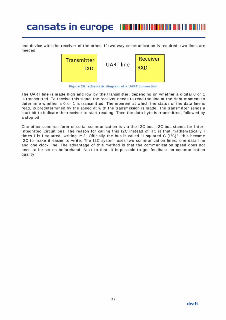
one device with the receiver of the other. If two-way communication is required, two lines are needed.

TXD RXDTransmitter Receiver

UART line

Figure 26: schematic diagram of a UART connection

The UART line is made high and low by the transmitter, depending on whether a digital 0 or 1 is transmitted. To receive this signal the receiver needs to read the line at the right moment to determine whether a 0 or 1 is transmitted. The moment at which the status of the data line is read, is predetermined by the speed at with the transmission is made. The transmitter sends a start bit to indicate the receiver to start reading. Then the data byte is transmitted, followed by a stop bit. One other common form of serial communication is via the I2C bus. I2C bus stands for Inter-Integrated Circuit bus. The reason for calling this I2C instead of IIC is that mathematically I times I is I squared, writing I^2. Officially the bus is called “I squared C (I2C)”, this became I2C to make it easier to write. The I2C system uses two communication lines; one data line and one clock line. The advantage of this method is that the communication speed does not need to be set on beforehand. Next to that, it is possible to get feedback on communication quality.

37

8 INTRODUCTION TO SOLDERING AND CIRCUIT ASSEMBLY

With a schematic diagram of an electric circuit completed it is time to go from theory to practice. To build an electric circuit, you need the components and a Printed Circuit Board (PCB) to place them on. The PCB can either be one especially made for your circuit, or a general PCB on which you make the connections of your circuit yourself. This chapter will first show some component placement and connection methods for nonspecific PCB’s. The design of custom made PCB’s is not part of this document, although some possible advantages will be addressed. The last part of this chapter will provide a short introduction and checking method for soldering of the components. A general form of nonspecific PCB’s is the experimentation PCB with a solder grid. The most general version has a grid of holes with a spacing of 2.54 mm, or 100 mil. Every hole is surrounded by a bit of copper to solder the components. A circuit is built on such PCB by placing the components on the board and then using wires to connect them. These wires need to be placed such that the connections of the schematic diagram and built circuit are the same. Using short wires is better than long wires. The longer a wire, the more resistance it has. If the wire resistance becomes high it will influence the circuit and result in unwanted behavior.

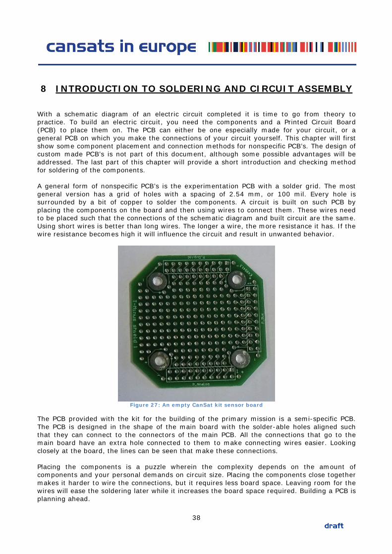
Figure 27: An empty CanSat kit sensor board

The PCB provided with the kit for the building of the primary mission is a semi-specific PCB. The PCB is designed in the shape of the main board with the solder-able holes aligned such that they can connect to the connectors of the main PCB. All the connections that go to the main board have an extra hole connected to them to make connecting wires easier. Looking closely at the board, the lines can be seen that make these connections. Placing the components is a puzzle wherein the complexity depends on the amount of components and your personal demands on circuit size. Placing the components close together makes it harder to wire the connections, but it requires less board space. Leaving room for the wires will ease the soldering later while it increases the board space required. Building a PCB is planning ahead.

38

Design of a dedicated PCB is a method to make soldering much simpler and creates less of a hassle with wires to connect everything. Making a specific design provides more flexibility in the components that can be used. On the general PCB the grid is 2.54 mm, but most of the modern components are much smaller than that. There are many programs available for making PCB’s. One that has a free license for non-commercial use is the computer program “Eagle”. After the PCB is designed in such a program, it needs to be fabricated. This fabrication can be done by dedicated factories.

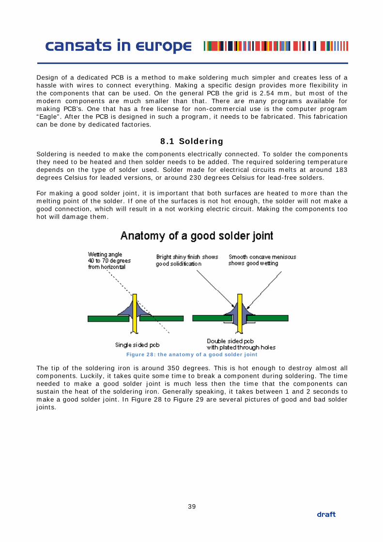
8.1 Soldering Soldering is needed to make the components electrically connected. To solder the components they need to be heated and then solder needs to be added. The required soldering temperature depends on the type of solder used. Solder made for electrical circuits melts at around 183 degrees Celsius for leaded versions, or around 230 degrees Celsius for lead-free solders. For making a good solder joint, it is important that both surfaces are heated to more than the melting point of the solder. If one of the surfaces is not hot enough, the solder will not make a good connection, which will result in a not working electric circuit. Making the components too hot will damage them.

Figure 28: the anatomy of a good solder joint

The tip of the soldering iron is around 350 degrees. This is hot enough to destroy almost all components. Luckily, it takes quite some time to break a component during soldering. The time needed to make a good solder joint is much less then the time that the components can sustain the heat of the soldering iron. Generally speaking, it takes between 1 and 2 seconds to make a good solder joint. In Figure 28 to Figure 29 are several pictures of good and bad solder joints.

39

Figure 29: drawing of good and bad solder joint

Figure 30: photographs of bad soldering (courtesy of T-Minus)

Figure 31: photographs of good soldering (courtesy of T-Minus)

40

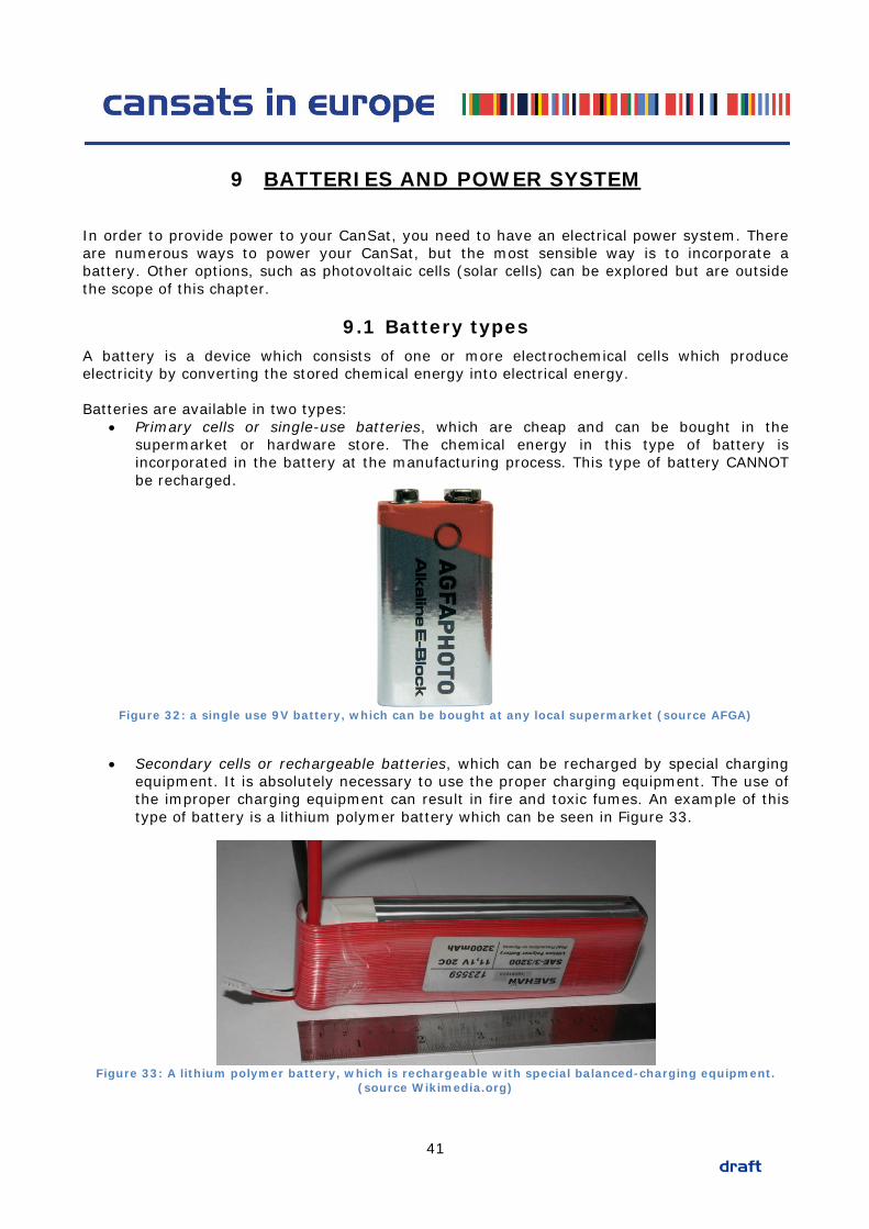
9 BATTERIES AND POWER SYSTEM

In order to provide power to your CanSat, you need to have an electrical power system. There are numerous ways to power your CanSat, but the most sensible way is to incorporate a battery. Other options, such as photovoltaic cells (solar cells) can be explored but are outside the scope of this chapter.

9.1 Battery types A battery is a device which consists of one or more electrochemical cells which produce electricity by converting the stored chemical energy into electrical energy. Batteries are available in two types:

• Primary cells or single-use batteries, which are cheap and can be bought in the supermarket or hardware store. The chemical energy in this type of battery is incorporated in the battery at the manufacturing process. This type of battery CANNOT be recharged.

Figure 32: a single use 9V battery, which can be bought at any local supermarket (source AFGA)

• Secondary cells or rechargeable batteries, which can be recharged by special charging

equipment. It is absolutely necessary to use the proper charging equipment. The use of the improper charging equipment can result in fire and toxic fumes. An example of this type of battery is a lithium polymer battery which can be seen in Figure 33.

Figure 33: A lithium polymer battery, which is rechargeable with special balanced-charging equipment.

(source Wikimedia.org)

41

9.2 Advantages and disadvantages The rechargeable battery has several advantages and disadvantages with respect to a single use battery. It depends on the requirements you have on a battery which battery you will need for your CanSat. Some considerations for choosing a battery type may be:

• A rechargeable battery can obviously be recharged during the project, which could result in a cost saving, because you do not need to buy new single-use batteries all the time.

• The energy density of a rechargeable battery is higher than a single use battery. This

means that for example 100 grams of rechargeable battery can contain more energy than 100 grams of single use battery. This is a very important factor in aerospace engineering, where every gram counts!

• The disadvantage of the rechargeable battery is that you will need special charging

equipment to charge your battery. This can be (very) expensive. Charging a battery can be dangerous, so always charge your battery on a non-combustible surface and never let it be unsupervised.

• Note: ALWAYS come to the launch site with fully charged batteries, or a fresh single use

battery.

9.3 Calculations with a battery The ESA CanSat kit needs voltages between 5.5V and 15V and has a power requirement of approximately 80 mA depending on the operation and the connected sensors. When a device which needs 80 mA is connected to for example a battery of 550 mAh, this means that it can run for . Of course, this will just be a rough estimation, since other factors, like resistance, current, battery internal resistance, battery temperature, etc. influence the actual battery lifetime. In general, the battery output voltage will drop during the lifetime of the battery. This is highly dependent on the amount of current that is consumed. Battery datasheets provide good reference for several types of current loading. The standard CanSat kit is powered by a simple single use 9V primary cell, of which specifications can be found in Figure 34.

9.4 Battery tips and tricks Having a good, stable and reliable voltage supply is absolutely essential for having a good and reliable CanSat. The CanSat electronics will only work when they are supplied with enough power. If the voltage drops only a fraction of a second under the 5.5V, strange things can happen, such as resetting microcontrollers or loss of signal. Make sure that the battery of the CanSat is fixed properly in the CanSat so that the battery leads are not momentarily disconnected when the rocket is accelerating, or the parachute is deployed with a high shock. Another thing that could happen is that some subsystems of your CanSat (momentarily) use a lot of power. Due to this high power consumption, the voltage that the battery supplies to the system drops, which can result for instance in a reset of one or more microcontrollers.

42

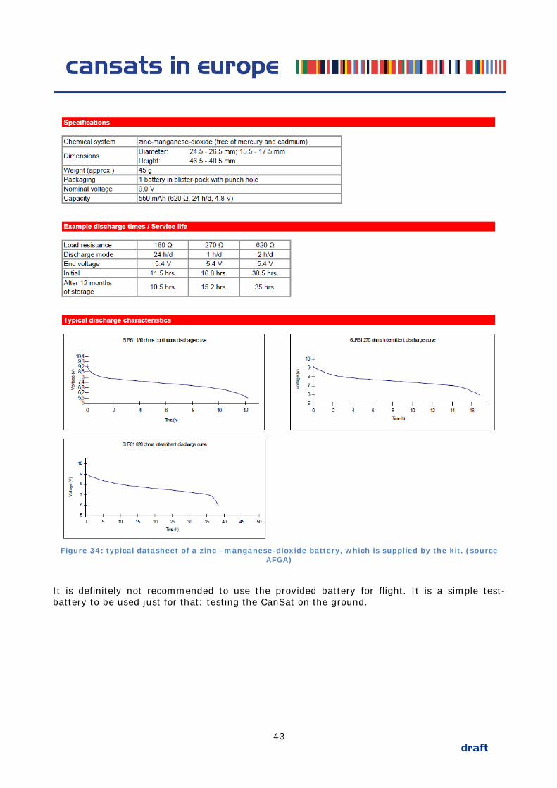
Figure 34: typical datasheet of a zinc –manganese-dioxide battery, which is supplied by the kit. (source

AFGA)

It is definitely not recommended to use the provided battery for flight. It is a simple test-battery to be used just for that: testing the CanSat on the ground.

43

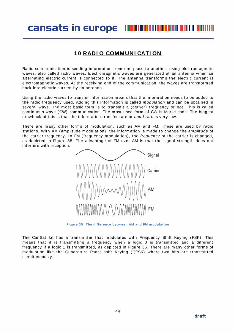
10 RADIO COMMUNICATION

Radio communication is sending information from one place to another, using electromagnetic waves, also called radio waves. Electromagnetic waves are generated at an antenna when an alternating electric current is connected to it. The antenna transforms the electric current is electromagnetic waves. At the receiving end of the communication, the waves are transformed back into electric current by an antenna. Using the radio waves to transfer information means that the information needs to be added to the radio frequency used. Adding this information is called modulation and can be obtained in several ways. The most basic form is to transmit a (carrier) frequency or not. This is called continuous wave (CW) communication. The most used form of CW is Morse code. The biggest drawback of this is that the information transfer rate or baud rate is very low. There are many other forms of modulation, such as AM and FM. These are used by radio stations. With AM (amplitude modulation), the information is made to change the amplitude of the carrier frequency. In FM (frequency modulation), the frequency of the carrier is changed, as depicted in Figure 35. The advantage of FM over AM is that the signal strength does not interfere with reception.

Figure 35: The difference between AM and FM modulation

The CanSat kit has a transmitter that modulates with Frequency Shift Keying (FSK). This means that it is transmitting a frequency when a logic 0 is transmitted and a different frequency if a logic 1 is transmitted, as depicted in Figure 36. There are many other forms of modulation like the Quadrature Phase-shift Keying (QPSK) where two bits are transmitted simultaneously.

44

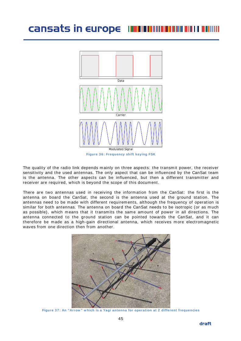
Figure 36: Frequency shift keying FSK

The quality of the radio link depends mainly on three aspects: the transmit power, the receiver sensitivity and the used antennas. The only aspect that can be influenced by the CanSat team is the antenna. The other aspects can be influenced, but then a different transmitter and receiver are required, which is beyond the scope of this document. There are two antennas used in receiving the information from the CanSat: the first is the antenna on board the CanSat, the second is the antenna used at the ground station. The antennas need to be made with different requirements, although the frequency of operation is similar for both antennas. The antenna on board the CanSat needs to be isotropic (or as much as possible), which means that it transmits the same amount of power in all directions. The antenna connected to the ground station can be pointed towards the CanSat, and it can therefore be made as a high-gain directional antenna, which receives more electromagnetic waves from one direction then from another.

Figure 37: An “Arrow” which is a Yagi antenna for operation at 2 different frequencies

45

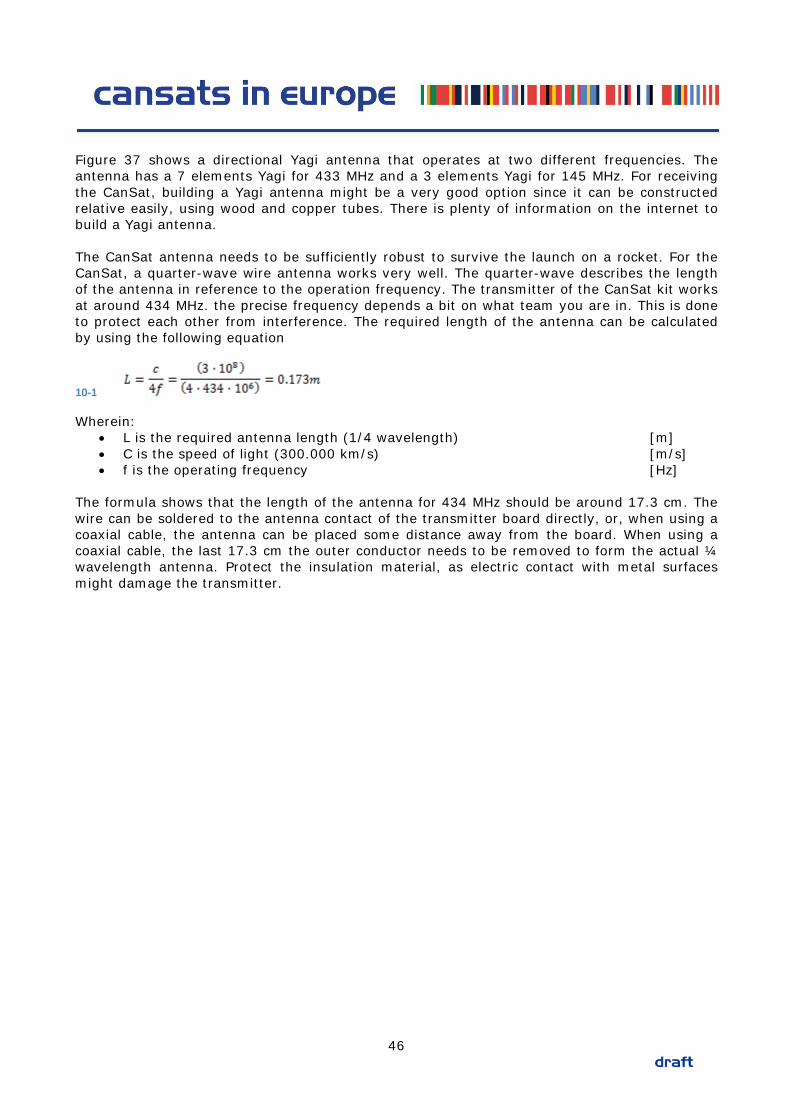
Figure 37 shows a directional Yagi antenna that operates at two different frequencies. The antenna has a 7 elements Yagi for 433 MHz and a 3 elements Yagi for 145 MHz. For receiving the CanSat, building a Yagi antenna might be a very good option since it can be constructed relative easily, using wood and copper tubes. There is plenty of information on the internet to build a Yagi antenna. The CanSat antenna needs to be sufficiently robust to survive the launch on a rocket. For the CanSat, a quarter-wave wire antenna works very well. The quarter-wave describes the length of the antenna in reference to the operation frequency. The transmitter of the CanSat kit works at around 434 MHz. the precise frequency depends a bit on what team you are in. This is done to protect each other from interference. The required length of the antenna can be calculated by using the following equation

10-1

Wherein: • L is the required antenna length (1/4 wavelength) [m] • C is the speed of light (300.000 km/s) [m/s] • f is the operating frequency [Hz]

The formula shows that the length of the antenna for 434 MHz should be around 17.3 cm. The wire can be soldered to the antenna contact of the transmitter board directly, or, when using a coaxial cable, the antenna can be placed some distance away from the board. When using a coaxial cable, the last 17.3 cm the outer conductor needs to be removed to form the actual ¼ wavelength antenna. Protect the insulation material, as electric contact with metal surfaces might damage the transmitter.

46

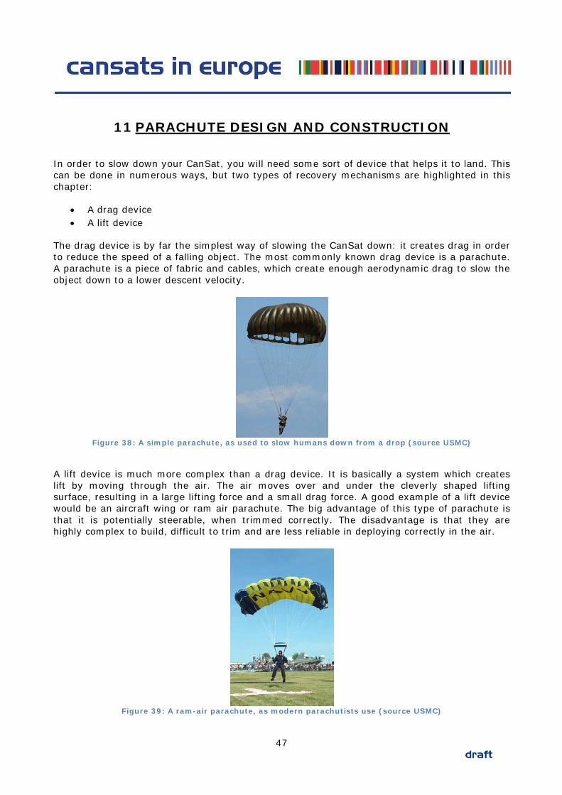
11 PARACHUTE DESIGN AND CONSTRUCTION

In order to slow down your CanSat, you will need some sort of device that helps it to land. This can be done in numerous ways, but two types of recovery mechanisms are highlighted in this chapter:

• A drag device • A lift device

The drag device is by far the simplest way of slowing the CanSat down: it creates drag in order to reduce the speed of a falling object. The most commonly known drag device is a parachute. A parachute is a piece of fabric and cables, which create enough aerodynamic drag to slow the object down to a lower descent velocity.

Figure 38: A simple parachute, as used to slow humans down from a drop (source USMC)

A lift device is much more complex than a drag device. It is basically a system which creates lift by moving through the air. The air moves over and under the cleverly shaped lifting surface, resulting in a large lifting force and a small drag force. A good example of a lift device would be an aircraft wing or ram air parachute. The big advantage of this type of parachute is that it is potentially steerable, when trimmed correctly. The disadvantage is that they are highly complex to build, difficult to trim and are less reliable in deploying correctly in the air.

Figure 39: A ram-air parachute, as modern parachutists use (source USMC)

47

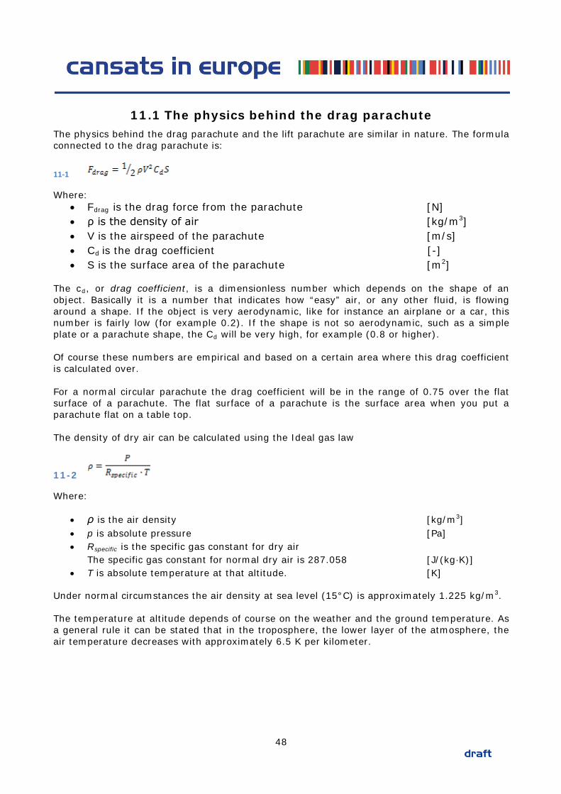
11.1 The physics behind the drag parachute The physics behind the drag parachute and the lift parachute are similar in nature. The formula connected to the drag parachute is:

11-1

Where: • Fdrag is the drag force from the parachute [N] • ρ is the density of air [kg/m3] • V is the airspeed of the parachute [m/s] • Cd is the drag coefficient [-] • S is the surface area of the parachute [m2]

The cd, or drag coefficient, is a dimensionless number which depends on the shape of an object. Basically it is a number that indicates how “easy” air, or any other fluid, is flowing around a shape. If the object is very aerodynamic, like for instance an airplane or a car, this number is fairly low (for example 0.2). If the shape is not so aerodynamic, such as a simple plate or a parachute shape, the Cd will be very high, for example (0.8 or higher). Of course these numbers are empirical and based on a certain area where this drag coefficient is calculated over. For a normal circular parachute the drag coefficient will be in the range of 0.75 over the flat surface of a parachute. The flat surface of a parachute is the surface area when you put a parachute flat on a table top. The density of dry air can be calculated using the Ideal gas law

11-2

Where:

• ρ is the air density [kg/m3] • p is absolute pressure [Pa] • Rspecific is the specific gas constant for dry air

The specific gas constant for normal dry air is 287.058 [J/(kg·K)] • T is absolute temperature at that altitude. [K]

Under normal circumstances the air density at sea level (15°C) is approximately 1.225 kg/m3. The temperature at altitude depends of course on the weather and the ground temperature. As a general rule it can be stated that in the troposphere, the lower layer of the atmosphere, the air temperature decreases with approximately 6.5 K per kilometer.

48

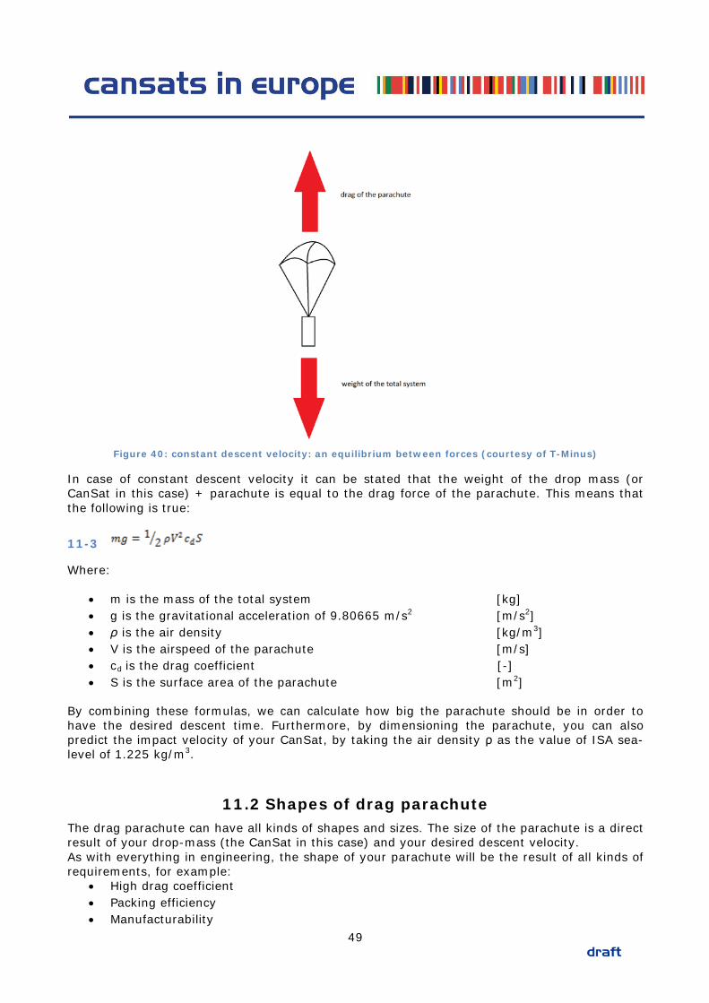
Figure 40: constant descent velocity: an equilibrium between forces (courtesy of T-Minus)

In case of constant descent velocity it can be stated that the weight of the drop mass (or CanSat in this case) + parachute is equal to the drag force of the parachute. This means that the following is true:

11-3

Where:

• m is the mass of the total system [kg] • g is the gravitational acceleration of 9.80665 m/s2 [m/s2] • ρ is the air density [kg/m3] • V is the airspeed of the parachute [m/s] • cd is the drag coefficient [-] • S is the surface area of the parachute [m2]

By combining these formulas, we can calculate how big the parachute should be in order to have the desired descent time. Furthermore, by dimensioning the parachute, you can also predict the impact velocity of your CanSat, by taking the air density ρ as the value of ISA sea-level of 1.225 kg/m3.

11.2 Shapes of drag parachute The drag parachute can have all kinds of shapes and sizes. The size of the parachute is a direct result of your drop-mass (the CanSat in this case) and your desired descent velocity. As with everything in engineering, the shape of your parachute will be the result of all kinds of requirements, for example:

• High drag coefficient • Packing efficiency • Manufacturability

49

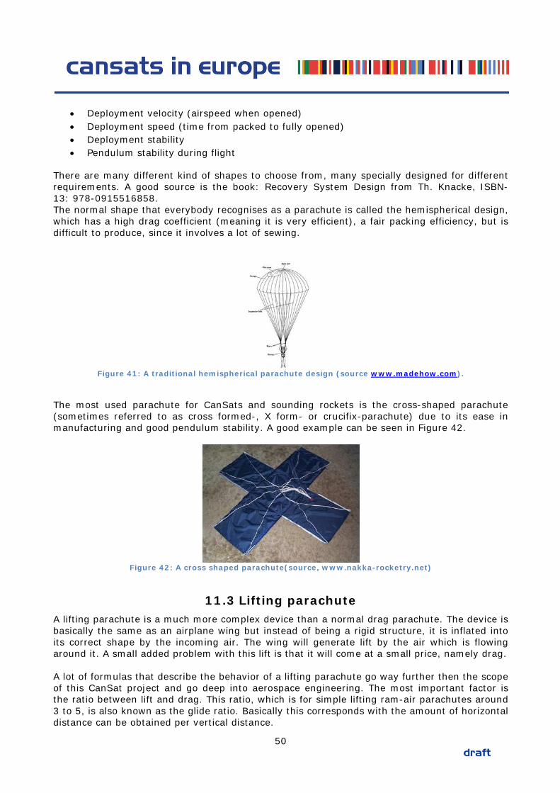
• Deployment velocity (airspeed when opened) • Deployment speed (time from packed to fully opened) • Deployment stability • Pendulum stability during flight

There are many different kind of shapes to choose from, many specially designed for different requirements. A good source is the book: Recovery System Design from Th. Knacke, ISBN-13: 978-0915516858. The normal shape that everybody recognises as a parachute is called the hemispherical design, which has a high drag coefficient (meaning it is very efficient), a fair packing efficiency, but is difficult to produce, since it involves a lot of sewing.

Figure 41: A traditional hemispherical parachute design (source www.madehow.com).

The most used parachute for CanSats and sounding rockets is the cross-shaped parachute (sometimes referred to as cross formed-, X form- or crucifix-parachute) due to its ease in manufacturing and good pendulum stability. A good example can be seen in Figure 42.

Figure 42: A cross shaped parachute(source, www.nakka-rocketry.net)

11.3 Lifting parachute A lifting parachute is a much more complex device than a normal drag parachute. The device is basically the same as an airplane wing but instead of being a rigid structure, it is inflated into its correct shape by the incoming air. The wing will generate lift by the air which is flowing around it. A small added problem with this lift is that it will come at a small price, namely drag. A lot of formulas that describe the behavior of a lifting parachute go way further then the scope of this CanSat project and go deep into aerospace engineering. The most important factor is the ratio between lift and drag. This ratio, which is for simple lifting ram-air parachutes around 3 to 5, is also known as the glide ratio. Basically this corresponds with the amount of horizontal distance can be obtained per vertical distance.

50

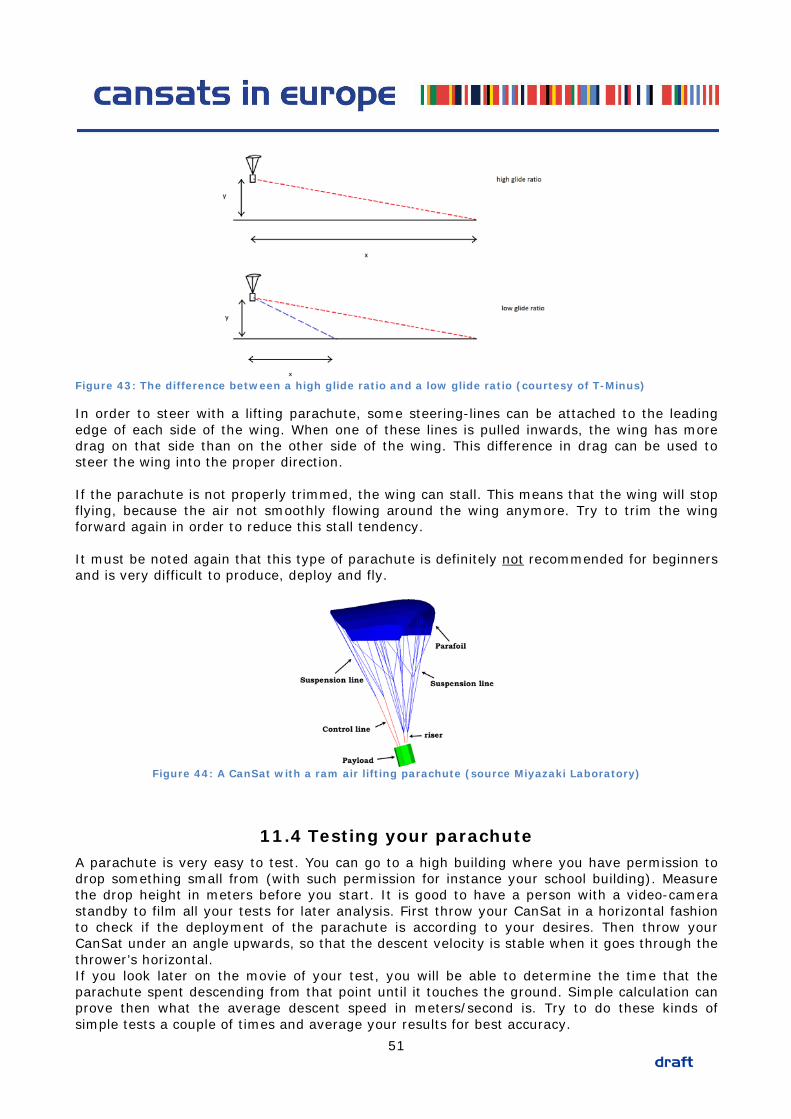
Figure 43: The difference between a high glide ratio and a low glide ratio (courtesy of T-Minus)

In order to steer with a lifting parachute, some steering-lines can be attached to the leading edge of each side of the wing. When one of these lines is pulled inwards, the wing has more drag on that side than on the other side of the wing. This difference in drag can be used to steer the wing into the proper direction. If the parachute is not properly trimmed, the wing can stall. This means that the wing will stop flying, because the air not smoothly flowing around the wing anymore. Try to trim the wing forward again in order to reduce this stall tendency. It must be noted again that this type of parachute is definitely not recommended for beginners and is very difficult to produce, deploy and fly.

Figure 44: A CanSat with a ram air lifting parachute (source Miyazaki Laboratory)

11.4 Testing your parachute A parachute is very easy to test. You can go to a high building where you have permission to drop something small from (with such permission for instance your school building). Measure the drop height in meters before you start. It is good to have a person with a video-camera standby to film all your tests for later analysis. First throw your CanSat in a horizontal fashion to check if the deployment of the parachute is according to your desires. Then throw your CanSat under an angle upwards, so that the descent velocity is stable when it goes through the thrower’s horizontal. If you look later on the movie of your test, you will be able to determine the time that the parachute spent descending from that point until it touches the ground. Simple calculation can prove then what the average descent speed in meters/second is. Try to do these kinds of simple tests a couple of times and average your results for best accuracy.

51

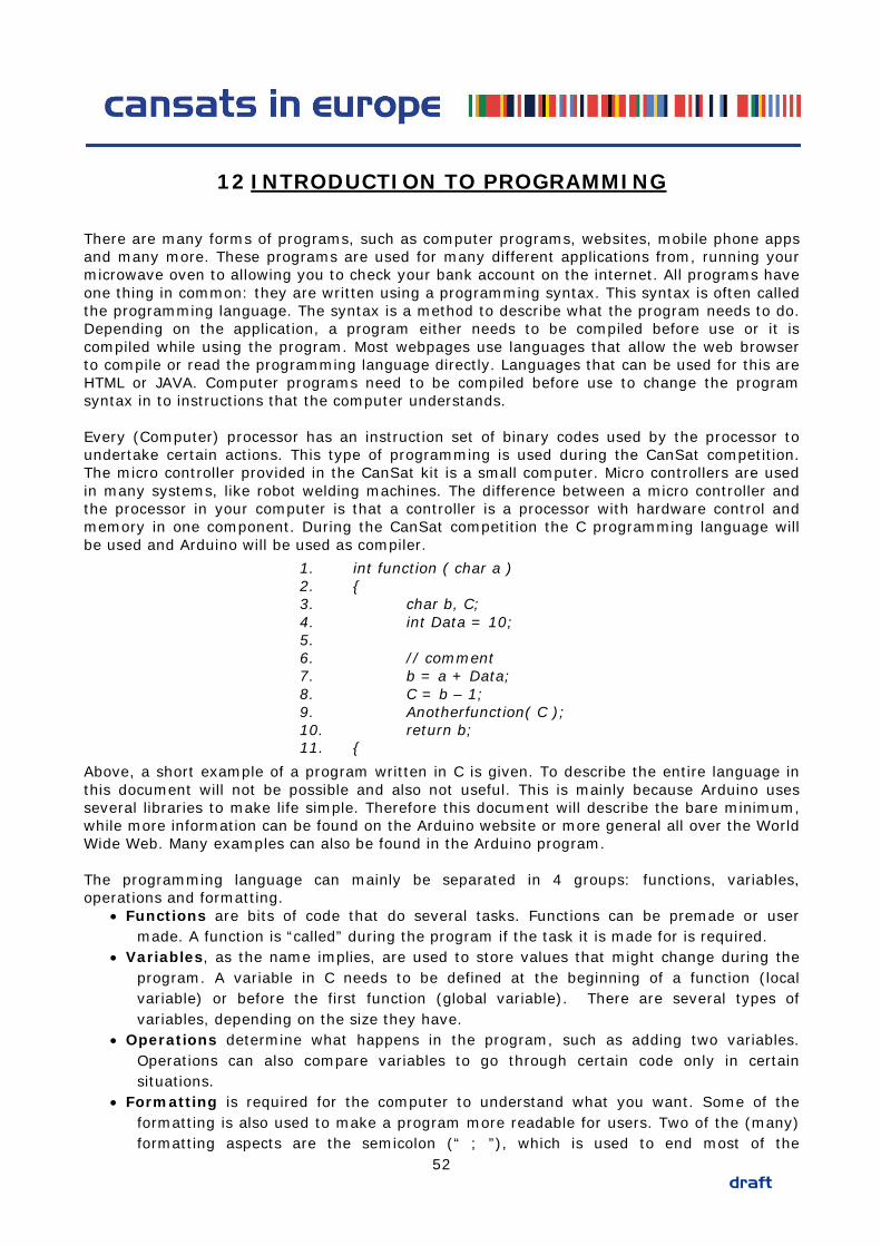
12 INTRODUCTION TO PROGRAMMING

There are many forms of programs, such as computer programs, websites, mobile phone apps and many more. These programs are used for many different applications from, running your microwave oven to allowing you to check your bank account on the internet. All programs have one thing in common: they are written using a programming syntax. This syntax is often called the programming language. The syntax is a method to describe what the program needs to do. Depending on the application, a program either needs to be compiled before use or it is compiled while using the program. Most webpages use languages that allow the web browser to compile or read the programming language directly. Languages that can be used for this are HTML or JAVA. Computer programs need to be compiled before use to change the program syntax in to instructions that the computer understands. Every (Computer) processor has an instruction set of binary codes used by the processor to undertake certain actions. This type of programming is used during the CanSat competition. The micro controller provided in the CanSat kit is a small computer. Micro controllers are used in many systems, like robot welding machines. The difference between a micro controller and the processor in your computer is that a controller is a processor with hardware control and memory in one component. During the CanSat competition the C programming language will be used and Arduino will be used as compiler.

Above, a short example of a program written in C is given. To describe the entire language in this document will not be possible and also not useful. This is mainly because Arduino uses several libraries to make life simple. Therefore this document will describe the bare minimum, while more information can be found on the Arduino website or more general all over the World Wide Web. Many examples can also be found in the Arduino program. The programming language can mainly be separated in 4 groups: functions, variables, operations and formatting.

• Functions are bits of code that do several tasks. Functions can be premade or user made. A function is “called” during the program if the task it is made for is required.

• Variables, as the name implies, are used to store values that might change during the program. A variable in C needs to be defined at the beginning of a function (local variable) or before the first function (global variable). There are several types of variables, depending on the size they have.

• Operations determine what happens in the program, such as adding two variables. Operations can also compare variables to go through certain code only in certain situations.

• Formatting is required for the computer to understand what you want. Some of the formatting is also used to make a program more readable for users. Two of the (many) formatting aspects are the semicolon (“ ; ”), which is used to end most of the

1. int function ( char a ) 2. 3. char b, C; 4. int Data = 10; 5. 6. // comment 7. b = a + Data; 8. C = b – 1; 9. Anotherfunction( C ); 10. return b; 11.

52

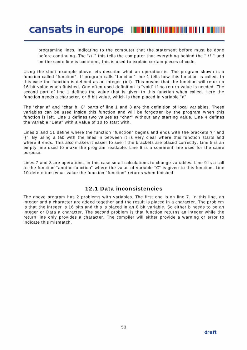
programing lines, indicating to the computer that the statement before must be done before continuing. The “// ” this tells the computer that everything behind the “ // “ and on the same line is comment, this is used to explain certain pieces of code.

Using the short example above lets describe what an operation is. The program shown is a function called “function”. If program calls “function” line 1 tells how this function is called. In this case the function is defined as an integer (int). This means that the function will return a 16 bit value when finished. One often used definition is “void” if no return value is needed. The second part of line 1 defines the value that is given to this function when called. Here the function needs a character, or 8 bit value, which is then placed in variable “a”. The “char a” and “char b, C” parts of line 1 and 3 are the definition of local variables. These variables can be used inside this function and will be forgotten by the program when this function is left. Line 3 defines two values as “char” without any starting value. Line 4 defines the variable “Data” with a value of 10 to start with. Lines 2 and 11 define where the function “function” begins and ends with the brackets ‘‘ and ‘’. By using a tab with the lines in between it is very clear where this function starts and where it ends. This also makes it easier to see if the brackets are placed correctly. Line 5 is an empty line used to make the program readable. Line 6 is a comment line used for the same purpose. Lines 7 and 8 are operations, in this case small calculations to change variables. Line 9 is a call to the function “anotherfunction” where the value of variable “C” is given to this function. Line 10 determines what value the function “function” returns when finished.

12.1 Data inconsistencies The above program has 2 problems with variables. The first one is on line 7. In this line, an integer and a character are added together and the result is placed in a character. The problem is that the integer is 16 bits and this is placed in an 8 bit variable. So either b needs to be an integer or Data a character. The second problem is that function returns an integer while the return line only provides a character. The compiler will either provide a warning or error to indicate this mismatch.

53

13 INTRODUCTION TO DATA ANALYSIS

At this point, you are at the stage where your CanSat is fully operational. You are able to perform measurements with the sensors and your CanSat can send the measurement data down to your ground station, where they are received. If everything went well, you received a stream of data lines. Each line consists of a time mark, indicating when the measurement was taken, and some numeric values of the voltages that your sensors recorded. From this data set, you want to deduce the actual quantities that your sensors measured, such as pressure and temperature. Then you want to present these quantities in a nice and clear way. This chapter provides you with guidelines on how to perform these steps.

13.1 From data to measurements: calibration The data received so far do not provide good insight into the quantities that are actually measured, such as air temperature: they are just voltages as obtained from the sensor outputs. To obtain valuable measurements, the voltages will have to be converted into the measured quantity. This can be done by determining a calibration curve for the sensor. A calibration curve essentially tells what output voltage can be expected when the sensor is subjected to a given temperature. This means that the curve can be used in the reversed way as well: it tells you what temperature the sensor senses when the output voltage is a given value. Therefore, measurements can be deduced from the data with this curve. In most cases, the relation between the sensed quantity and the output voltage is linear, which means that it can be expressed as: 13-1 meas outQ a V b= ⋅ +

Where

• Qmeas is the value of the measured quantity (for example temperature) [K]

• Vout is the output voltage of the sensor [V] • a is the calibration gradient [K/V] • b is the calibration offset [K]

Calibration of the sensor means therefore determining the values of a and b. For some sensors, this is very easy: just check the data sheet of the sensor. The gradient and offset should be given there. However, in most cases, only a range of values is given: the gradient and offset may be in between a certain minimum and maximum value. Determining the exact values is therefore necessary. The equipment needed to perform a calibration is a source of the quantity that is measured (for the temperature sensor, this is a device that can give the sensor a given, well-defined temperature, for example a glass with water on a hot plate), and a pre-calibrated sensor, such as a thermometer. The thermometer and the sensor are both placed in the glass of water and the output from the sensor as well as the indicated temperature on the thermometer is monitored and noted down. Now, the temperature of the water is gradually increased by turning on the hot plate. At given time intervals, both the sensor output and the reading from the thermometer are noted. The calibration can be stopped when 5 – 10 measurement within

54

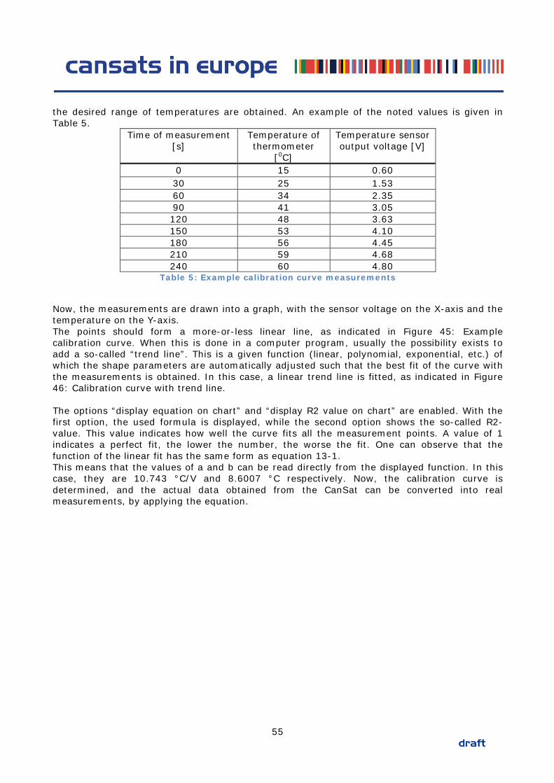
the desired range of temperatures are obtained. An example of the noted values is given in Table 5.

Time of measurement [s]

Temperature of thermometer

[0C]

Temperature sensor output voltage [V]

0 15 0.60 30 25 1.53 60 34 2.35 90 41 3.05 120 48 3.63 150 53 4.10 180 56 4.45 210 59 4.68 240 60 4.80

Table 5: Example calibration curve measurements

Now, the measurements are drawn into a graph, with the sensor voltage on the X-axis and the temperature on the Y-axis. The points should form a more-or-less linear line, as indicated in Figure 45: Example calibration curve. When this is done in a computer program, usually the possibility exists to add a so-called “trend line”. This is a given function (linear, polynomial, exponential, etc.) of which the shape parameters are automatically adjusted such that the best fit of the curve with the measurements is obtained. In this case, a linear trend line is fitted, as indicated in Figure 46: Calibration curve with trend line. The options “display equation on chart” and “display R2 value on chart” are enabled. With the first option, the used formula is displayed, while the second option shows the so-called R2- value. This value indicates how well the curve fits all the measurement points. A value of 1 indicates a perfect fit, the lower the number, the worse the fit. One can observe that the function of the linear fit has the same form as equation 13-1. This means that the values of a and b can be read directly from the displayed function. In this case, they are 10.743 °C/V and 8.6007 °C respectively. Now, the calibration curve is determined, and the actual data obtained from the CanSat can be converted into real measurements, by applying the equation.

55

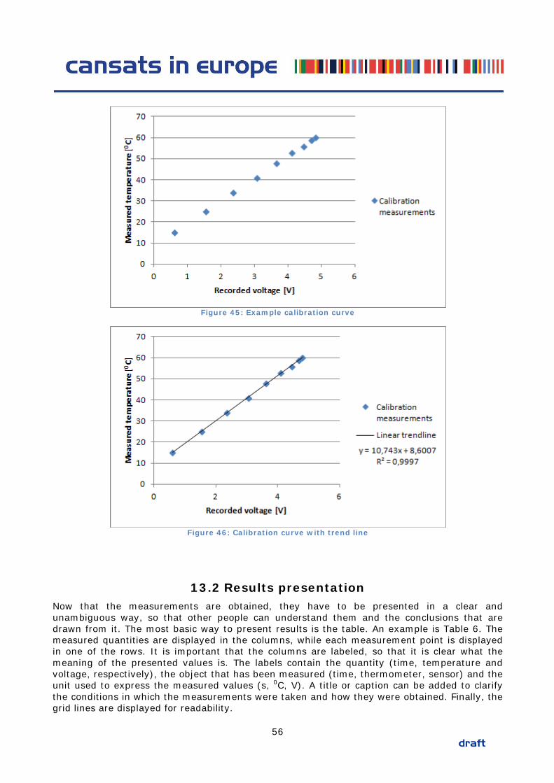
Figure 45: Example calibration curve

Figure 46: Calibration curve with trend line

13.2 Results presentation Now that the measurements are obtained, they have to be presented in a clear and unambiguous way, so that other people can understand them and the conclusions that are drawn from it. The most basic way to present results is the table. An example is Table 6. The measured quantities are displayed in the columns, while each measurement point is displayed in one of the rows. It is important that the columns are labeled, so that it is clear what the meaning of the presented values is. The labels contain the quantity (time, temperature and voltage, respectively), the object that has been measured (time, thermometer, sensor) and the unit used to express the measured values (s, 0C, V). A title or caption can be added to clarify the conditions in which the measurements were taken and how they were obtained. Finally, the grid lines are displayed for readability.

56

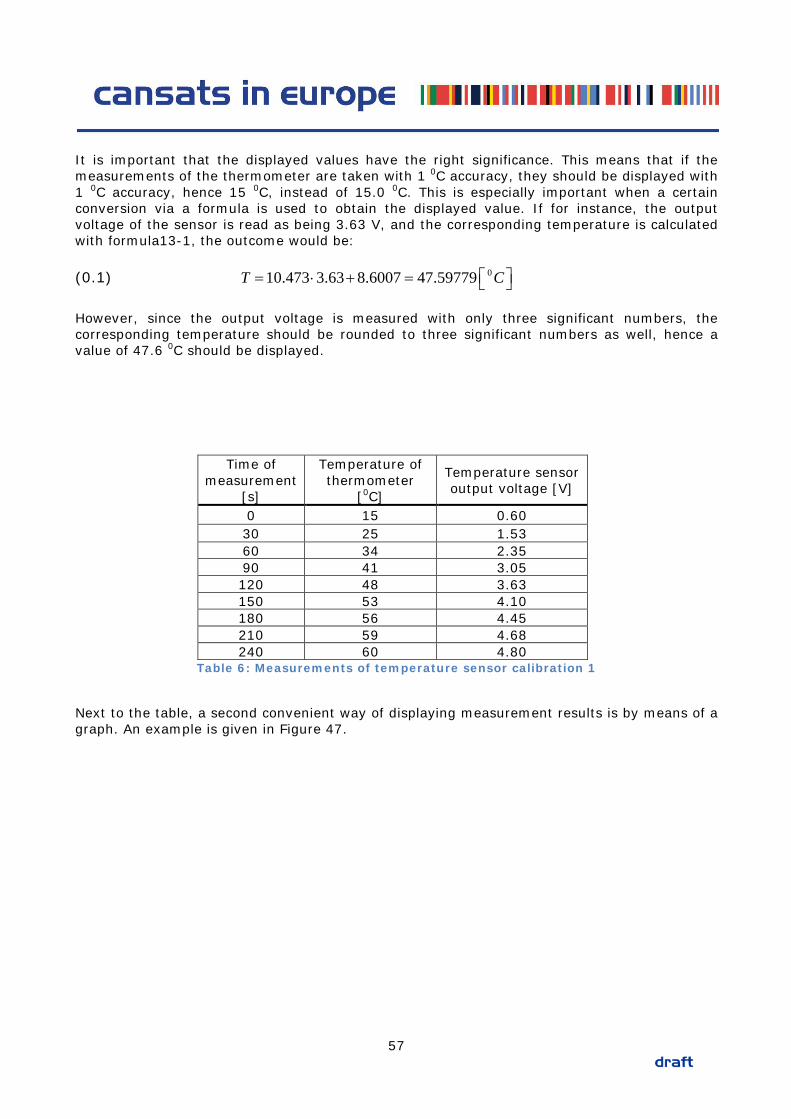
It is important that the displayed values have the right significance. This means that if the measurements of the thermometer are taken with 1 0C accuracy, they should be displayed with 1 0C accuracy, hence 15 0C, instead of 15.0 0C. This is especially important when a certain conversion via a formula is used to obtain the displayed value. If for instance, the output voltage of the sensor is read as being 3.63 V, and the corresponding temperature is calculated with formula13-1, the outcome would be: (0.1) 010.473 3.63 8.6007 47.59779T C = ⋅ + = However, since the output voltage is measured with only three significant numbers, the corresponding temperature should be rounded to three significant numbers as well, hence a value of 47.6 0C should be displayed.

Time of measurement

[s]

Temperature of thermometer

[0C]

Temperature sensor output voltage [V]

0 15 0.60 30 25 1.53 60 34 2.35 90 41 3.05 120 48 3.63 150 53 4.10 180 56 4.45 210 59 4.68 240 60 4.80

Table 6: Measurements of temperature sensor calibration 1

Next to the table, a second convenient way of displaying measurement results is by means of a graph. An example is given in Figure 47.

57

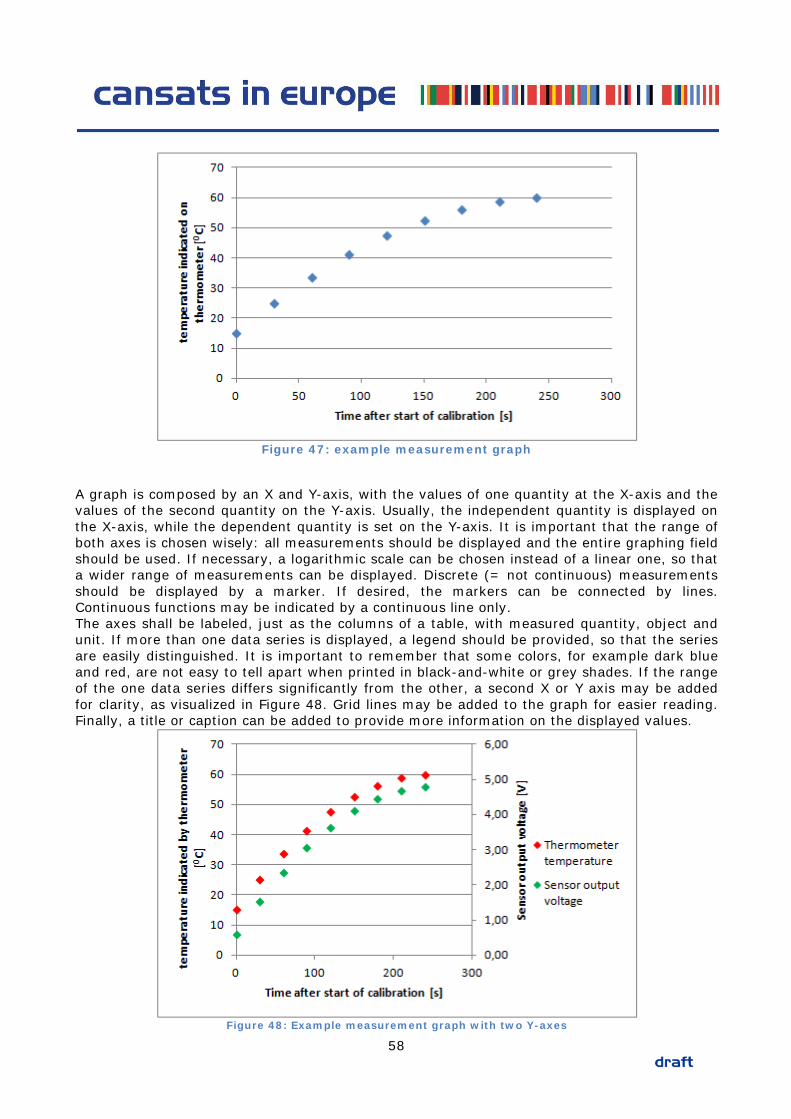
Figure 47: example measurement graph

A graph is composed by an X and Y-axis, with the values of one quantity at the X-axis and the values of the second quantity on the Y-axis. Usually, the independent quantity is displayed on the X-axis, while the dependent quantity is set on the Y-axis. It is important that the range of both axes is chosen wisely: all measurements should be displayed and the entire graphing field should be used. If necessary, a logarithmic scale can be chosen instead of a linear one, so that a wider range of measurements can be displayed. Discrete (= not continuous) measurements should be displayed by a marker. If desired, the markers can be connected by lines. Continuous functions may be indicated by a continuous line only. The axes shall be labeled, just as the columns of a table, with measured quantity, object and unit. If more than one data series is displayed, a legend should be provided, so that the series are easily distinguished. It is important to remember that some colors, for example dark blue and red, are not easy to tell apart when printed in black-and-white or grey shades. If the range of the one data series differs significantly from the other, a second X or Y axis may be added for clarity, as visualized in Figure 48. Grid lines may be added to the graph for easier reading. Finally, a title or caption can be added to provide more information on the displayed values.

Figure 48: Example measurement graph with two Y-axes

58

59

14 PRESENTATION, REPORTS AND BLOGS

In order to communicate in a large project, it is essential to have good presentation skills and a good, concise and clear reporting style. Both presentations and reporting are needed for your CanSat project. The FDR is needed to relay all project-information to the judges of the CanSat competition. Furthermore, a small presentation is needed to accompany this report that will explain what your project is about to people who did not read your report and did not follow your progress continuously.

14.1 Briefing and Debriefing presentations During the Launch Campaign, the competition winner will be decided based on the overall performance of the team. Each team must present the data obtained during the flight and the mission analysis. Each presentation should be concise and have no more than 10 slides. The presentation will contain:

• Introducing the team • General description of mission objectives • Description of the design • Brief introduction of the team • Graphics of the data obtained during the flight • Analysis of the data obtained • Success or failure analysis • Conclusions

Some tips to help you create a great PowerPoint Presentation:

• Do not put large amounts of text on the slides. • Do not read from the slides while you are presenting. • Create a clear and concise Power Point of 10-15 slides. • Use only information that is relevant to the subject you are presenting. • Use only one background throughout your presentation. • Stick to one font, keep it simple. • Keep transitions simple between slides. • Use pictures, diagrams, graphs wherever possible to illustrate your idea.

To give a presentation, for a lot of people, is something that everybody dislikes in the beginning. Some people really find it scary, but it is a skill that can be acquired very quickly. At first try to practice a couple of times what you want to say. Don’t learn your presentation “by heart”, because in the end you might rush your presentation or sound monotonous you do the final version in public. Some small tips for presenting:

• Try to be as relaxed and normal as possible. • Speak slowly, don’t try to rush everything to the end. If you have a watch or a small

clock, take it with you on the stage. You will directly see how much time you have left for your presentation. You can either slow down or accelerate if the time demands it.

• Know your stuff. If you did the research, you will be the person who knows everything there is to know. For questions about the subject you are the best person to answer it.

60

If you don’t know the answer then you can always say that it is a good question and you will look for an answer and contact the person after the presentation.

• Have fun. After a while you are not as scared anymore for speaking in public. Try to enjoy it, people in the audience will notice it and find it much easier to listen to it.

14.2 Reports For writing reports try to be as concise and to the point as possible. Do not use familiar language. Details are important as well but try to structure your ideas when writing your paper. Do not overload with electronic schematics, you can add them in an appendix. The document itself (without the appendices) should be a readable document for a technically educated person.

14.3 Team blog One important way for you to attract attention from the media, sponsors and your peers is to create your own blog. Writing a blog post has many different advantages depending on how you look at things. Whether you write every once in a while or once per week writing something is better than nothing and still has some advantages. Don’t be afraid to:

• To express your thoughts and opinions. You have something to say, and blogs provide a place to say it and be heard.

• To promote your team blogging is a great way to help market or promote your team. • To help people. Many blogs are written to help people who may be going through similar

situations like you have experienced. • To connect with people with the same interests. Blogging brings like-minded people

together. • To attract sponsors. You can post a logo or make an article about how a certain

business helped you in building your CanSat.

61

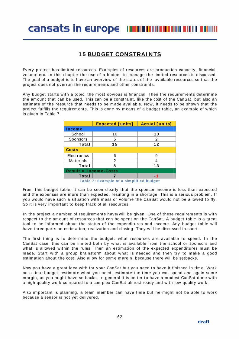
15 BUDGET CONSTRAINTS

Every project has limited resources. Examples of resources are production capacity, financial, volume,etc. In this chapter the use of a budget to manage the limited resources is discussed. The goal of a budget is to have an overview of the status of the available resources so that the project does not overrun the requirements and other constraints. Any budget starts with a topic, the most obvious is financial. Then the requirements determine the amount that can be used. This can be a constraint, like the cost of the CanSat, but also an estimate of the resource that needs to be made available. Now, it needs to be shown that the project fulfills the requirements. This is done by means of a budget table, an example of which is given in Table 7.

Expected [units] Actual [units] Income

School 10 10 Sponsors 5 2

Total 15 12 Costs Electronics 6 9 Materials 2 4

Total 8 13 Result = Income-Costs

Total 7 -1 Table 7: Example of a simplified budget

From this budget table, it can be seen clearly that the sponsor income is less than expected and the expenses are more than expected, resulting in a shortage. This is a serious problem. If you would have such a situation with mass or volume the CanSat would not be allowed to fly. So it is very important to keep track of all resources. In the project a number of requirements have/will be given. One of these requirements is with respect to the amount of resources that can be spent on the CanSat. A budget table is a great tool to be informed about the status of the expenditures and income. Any budget table will have three parts an estimation, realization and closing. They will be discussed in short. The first thing is to determine the budget: what resources are available to spend. In the CanSat case, this can be limited both by what is available from the school or sponsors and what is allowed within the rules. Then an estimation of the expected expenditures must be made. Start with a group brainstorm about what is needed and then try to make a good estimation about the cost. Also allow for some margin, because there will be setbacks. Now you have a great idea with for your CanSat but you need to have it finished in time. Work on a time budget; estimate what you need, estimate the time you can spend and again some margin, as you might have setbacks. In general it is better to have a modest CanSat done with a high quality work compared to a complex CanSat almost ready and with low quality work. Also important is planning, a team member can have time but he might not be able to work because a sensor is not yet delivered.

62

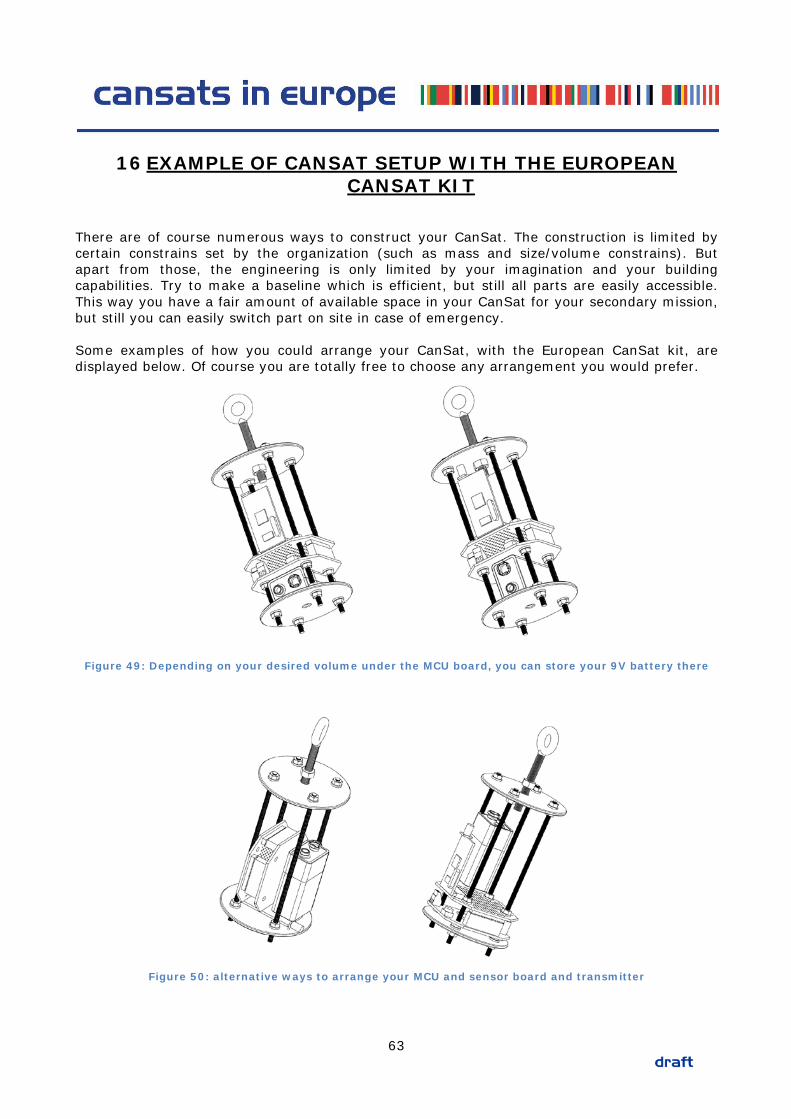
16 EXAMPLE OF CANSAT SETUP WITH THE EUROPEAN CANSAT KIT

There are of course numerous ways to construct your CanSat. The construction is limited by certain constrains set by the organization (such as mass and size/volume constrains). But apart from those, the engineering is only limited by your imagination and your building capabilities. Try to make a baseline which is efficient, but still all parts are easily accessible. This way you have a fair amount of available space in your CanSat for your secondary mission, but still you can easily switch part on site in case of emergency. Some examples of how you could arrange your CanSat, with the European CanSat kit, are displayed below. Of course you are totally free to choose any arrangement you would prefer.

Figure 49: Depending on your desired volume under the MCU board, you can store your 9V battery there

Figure 50: alternative ways to arrange your MCU and sensor board and transmitter

63

17 OTHER RESOURCES AND FURTHER INFORMATION

• http://upload.wikimedia.org/wikipedia/commons/0/07/Lithium_polymer_battery_%281

1.1_volts%29.jpg • http://www.produktinfo.conrad.com/datenblaetter/650000-674999/650411-da-01-en-

AGFAPHOTO_9V_E_BLOCK.pdf • http://www.conrad.nl/ce/nl/product/650411/ • http://upload.wikimedia.org/wikipedia/commons/e/e6/USMC_Paratrooper.jpg • http://en.wikipedia.org/wiki/File:Ram_air_square.jpg • http://forth.aero.cst.nihon-u.ac.jp/activity/e-a-pad.html • http://www.madehow.com/images/hpm_0000_0005_0_img0132.jpg • http://www.nakka-rocketry.net/xchute1.html • http://www.scienceprog.com/how-to-describe-embedded-software-design-using-

diagrams-and-pseudo-code/ • http://www.t-minus.nl/products/cansat-kit/

64