Signal Processing 101 (2014) 74–86

Contents lists available at ScienceDirect

Amplitu

the recties ov

http://d0165-16

n CorrE-m

sabrar@asoke.n

Signal Processing

journal homepage: www.elsevier.com/locate/sigpro

Newton-like minimum entropy equalization algorithmfor APSK systems

Anum Ali a,n, Shafayat Abrar b, Azzedine Zerguine a, Asoke K. Nandi c

a King Fahd University of Petroleum & Minerals, Dhahran 31261, Saudi Arabia

b COMSATS Institute of Information Technology, Islamabad, Pakistanc Brunel University, Uxbridge, Middlesex UB8 3PH, UK

& 2014 Elsevier B.V. All rights reserved.

a r t i c l e i n f o

Article history:Received 6 August 2013Received in revised form29 January 2014Accepted 5 February 2014Available online 13 February 2014

Keywords:Constant modulus algorithmBlind equalizerRecursive least squares algorithmNewton's method

de phase shift keying

eiver, except for its probabilistic or ser some known alphabets. As both th

x.doi.org/10.1016/j.sigpro.2014.02.00384 & 2014 Elsevier B.V. All rights reserved.

esponding author. Tel.: þ966 59 779 4592.ail addresses: anumali@ieee.org (A. Ali),comsats.edu.pk (S. Abrar), azzedine@kfupm.andi@brunel.ac.uk (A.K. Nandi).

a b s t r a c t

In this paper, we design and analyze a Newton-like blind equalization algorithm for theAPSK system. Specifically, we exploit the principle of minimum entropy deconvolutionand derive a blind equalization cost function for APSK signals and optimize it usingNewton's method. We study and evaluate the steady-state excess mean square errorperformance of the proposed algorithm using the concept of energy conservation.Numerical results depict a significant performance enhancement for the proposed schemeover well established blind equalization algorithms. Further, the analytical excess meansquare error of the proposed algorithm is verified with computer simulations and is foundto be in good conformation.

Tracking performance

1. Introduction

In digital communications at high enough data rates,almost all physical channels exhibit inter-symbol interfer-ence (ISI). One of the solutions to this problem is blindequalization, which is a method to equalize distortivecommunication channels and mitigate ISI without super-vision. Blind equalization algorithms do not require train-ing at either the startup period or restart after systembreakdown. This independence of blind schemes withrespect to training sequence results in improved systembandwidth efficiency.

In blind equalization, the desired signal is unknown to

tatistical proper-e channel and its

edu.sa (A. Zerguine),

input are unknown, the objective of blind equalization is torecover the unknown input sequence based solely on itsprobabilistic and statistical properties [1–3]. From the avail-able literature, it can be found that any admissible blindobjective (or cost) function has two main attributes: (1) itmakes use of the statistics which are significantly modifiedas the signal propagates through the channel [4] and(2) optimization of the cost function modifies the statisticsof the signal at the equalizer output, aligning them with thestatistics of the signal at the channel input [5].

One of the earliest methods of blind equalization wassuggested by Benveniste et al. [5]. Their proposed methodassumed the transmitted signal to be non-Gaussian, inde-pendent and identically distributed (i.i.d.) sequence of aknown statistical distribution. It sought to match the dis-tribution of its output (deconvolved sequence) with thedistribution of the transmitted signal and the adaptationcontinued until the said objective was achieved. Another

approach to this problem was devised by Donoho [4], whodefined a partial ordering, measuring the relative Gaussianity

ocessi

between random variables. He suggested to adjust theequalizer until the distribution of the deconvolved sequenceis as non-Gaussian as possible. A somewhat informal versionof Donoho's method appeared in the work of Wiggins [6,7].According to Wiggins, assuming the transmitted signal is anon-Gaussian signal with certain distribution pa, the equal-izer must be adjusted to make its output signal distributionresemble pa. He termed this approach as a minimum entropydeconvolution (MED) criterion.

In this work, the MED criterion is the subject of ourconcern for designing (and optimizing) cost functions toequalize signals blindly in amplitude phase shift keying(APSK) systems. The APSK signals are very important inmodern day communication systems due to their robustnessagainst nonlinear channel distortion and advantageous lowerpeak-to-average power ratio compared to the conventionalquadrature amplitude modulation signals (refer to APSKbased systems in [8–14] and references therein).

This paper is organized as follows: Section 2 discusses thebaseband communication system model, notion of Gaussian-ity, and traditional blind equalizers. Section 3 describes theMED criteria for channel equalization, discusses the admis-sibility of costs tailored for APSK, and stochastic gradient-based optimization. Section 4 formulates the proposedadaptive MED-based blind equalization scheme for APSKsystems exploiting Newton-like update. Section 5 provides asteady-state tracking performance of the proposed algorithm

A. Ali et al. / Signal Pr

in time varying scenario. Simulation results are discussed in

Section 6 and conclusions are provided in Section 7.

2. System model and traditional blind equalizers

The baseband model for a typical complex-valued datacommunication system, as shown in Fig. 1, consists of anunknown finite-impulse response filter hn, which repre-sents the physical inter-connection between the transmitterand the receiver. A zero-mean, i.i.d., circularly symmetric,complex-valued data sequence fang is transmitted throughthe channel, whose output xn is recorded by the receiver.The input/output relationship of the channel can be writtenas xn ¼∑kan�khkþνn; where the additive noise νn isassumed to be stationary, Gaussian, and independent ofthe channel input an. The function of equalizer at thereceiver is to estimate the delayed version of original data,an� τ , from the received signal xn. Let wn ¼ ½wn;0;wn;1;

…;wn;N�1�T be a vector of equalizer coefficients with Nelements and xn ¼ ½xn; xn�1;…; xn�Nþ1�T be the vector ofchannel observations (T denotes transpose operation). Theoutput of the equalizer is then given by yn ¼wH

n�1xn (H

denotes the Hermitian conjugate operator). If tn ¼ hn �wn

n�1 represents the overall channel-equalizer impulse

Fig. 1. A typical baseband communication system.

response (�denotes convolution), then

yn ¼∑iwn

n�1;ixn� i ¼ tn;τan� τþ ∑la τ

tn;lan� lþν 0n|fflfflfflfflfflfflfflfflfflfflfflfflfflfflfflfflfflfflfflfflfflffl{zfflfflfflfflfflfflfflfflfflfflfflfflfflfflfflfflfflfflfflfflfflffl}

signalþ ISIþnoise

ð1Þ

which demonstrates the adverse effect of inter-symbolinterference (ISI) and additive noise. The ISI is quantifiedas [15]:

ISI¼ ∑ijtn;ij2�maxfjtnj2gmaxfjtnj2g

ð2Þ

In subsequent discussions we drop the subscript n from t fornotational convenience. The idea behind a Bussgang blindequalizer is to minimize (or maximize), through the choiceof w, a certain cost function J depending on yn, such that ynprovides an estimate of an up to some inherent indetermi-nacies, giving, yn ¼ αan� τ , where α¼ jαjejθAC represents anarbitrary complex-valued gain. Hence, a Bussgang blindequalizer tries to solve the following optimization problem:

w† ¼ argw

optimize J with J ¼EJ ðynÞ ð3Þ

The cost J is a function of implicitly embedded statistics of ynand J ð�Þ is a real-valued function. Ideally, the cost J makesuse of statistics which are significantly modified as thesignal propagates through the channel, and the optimiza-tion of cost modifies the statistics of the signal at theequalizer output, aligning them with those at a channelinput. The equalization is accomplished when equalizedsequence yn acquires an identical distribution as that of thechannel input an. More formally, we have the followingtheorem [5]:

Theorem 1. If the transmitted signal is composed of non-Gaussian i.i.d. samples, both the channel and the equalizerare linear time-invariant filters, noise is negligible, and theprobability density functions (PDF) of transmitted and equal-ized signals are equal, then the channel has been perfectlyequalized.

This mathematical result is very important since itestablishes the possibility of obtaining an equalizer withthe sole aid of signal's statistical properties and withoutrequiring any knowledge of the channel impulse responseor training data sequence. Meanwhile, Donoho [4] notedthat, as a consequence of the central limit theorem, linearcombinations of identically distributed random variablesbecome more Gaussian than the individual variables.Therefore, the received signal xn will have a distributionthat is more nearly Gaussian than the distribution of an.Any suitable objective function capable of measuringGaussianity or non-Gaussianity can therefore be used fordeconvolution.

One of the measures of Gaussianity is (normalized)kurtosis, κ, which is a statistic based on second and fourth-order moments. For a circularly-symmetric complex-valued random variable X, kurtosis is defined as [15]:

κX ¼ Ejxj4ðEjxj2Þ2

�2 ð4Þ

ng 101 (2014) 74–86 75

κX is greater than zero, equal to zero, and less than zerofor super-Gaussian, Gaussian, and sub-Gaussian random

0 1 2 3 4 5 60

0.5

1

1.5

α

Ent

ropy

[in

nats

]

ocessing 101 (2014) 74–86

variables, respectively. Expectedly most of the existingblind equalizers use second and fourth-order statistics ofthe equalized sequence. The first ever method which relieson the aforesaid statistics is the constant modulus criter-ion [16]; it is given by

minw

fEjynj4�2R2Ejynj2g; ð5Þ

where R is the Godard radius and R2 ¼Ejanj4=Ejanj2 is theGodard dispersion constant [17]. For an input signal that hasa constant modulus janj ¼ R, the constant modulus criter-ion penalizes output samples yn that do not have thedesired constant modulus characteristics [18].

Shalvi and Weinstein [15] demonstrated that the con-dition of equality between the PDF of the transmitted andequalized signals, due to Theorem 1, was excessively tight.Under the similar assumptions, as laid in Theorem 1, theydiscussed the possibility to perform blind equalization bysatisfying the condition Ejynj2 ¼ Ejanj2 and ensuring that anonzero cumulant (of any order higher than 2) of an and ynare equal. For a two dimensional signal an with four-quadrant symmetry (i.e., Ea2n ¼ 0), they suggested to max-imize the following exemplary cost containing second andfourth-order statistics:

maxw

jEjynj4�2ðEjynj2Þ2j s:t: Ejynj2 ¼ Ejanj2 ð6Þ

In the next section, we discuss equalization/deconvolution

A. Ali et al. / Signal Pr76

techniques which evolved around the notion of entropy as

in the data [23]. Wiggins coined the term MED criterionfor the test (10).1 Immediately after Wiggins, Ooe and

1 The simple structure of the impulsive function led Wiggins to call

a measure of Gaussianity.

3. Minimum entropy deconvolution

In statistics, the most powerful test of the null hypoth-esis against another is one which maximizes discrimina-tion and minimizes the probability of accepting the nullhypothesis as true when actually the alternative is true.In information theory, a statistic that maximizes detect-ability of a signal while minimizing the probability of afalse alarm is most powerful. In seismic community,however, a statistical (rank-discriminating) test againstGaussianity, which can be used to design a deconvolutionfilter, is loosely termed as a MED criterion [4,6].

Hogg [19] developed a scale-invariant and the mostpowerful rank-discriminating test for one member of thegeneralized Gaussian against another by considering thefollowing PDF:

pY y; αð Þ ¼ α

2Γ1α

� � exp �jyjαð Þ; y o1j�� ð7Þ

where α40 is shape parameter, and Γð�Þ is the Gammafunction. To determine if a random set of samplesfy1; y2;…; yBg is drawn from the distribution pY ðy; α2Þ asopposed to pY ðy; α1Þ, a ratio test was derived (based on theprocedure described in [20]) as follows:

VY α1; α2ð Þ ¼1B∑B

i ¼ 1jyijα1� �B=α1

� �B=α2≷

α ¼ α2χ ð8Þ

1B∑B

i ¼ 1jyijα2α ¼ α1

where χ is some threshold. The larger V becomes, the moreprobable it is that the sample set Y is drawn from thedistribution pY ðy; α2Þ and not pY ðy; α1Þ.

It would be interesting to look at the entropy, HðαÞ,associated with (7); it is given as follows [21]:

H αð Þ ¼ log2α

ffiffiffiffiffiffiffiffiffiffiffiffiffiffiffiffiffiffiffiffiffiffiffiffiffiffiffiffiffiffiffiffiffiffiffiffiffiΓ

1α

� �3

Γ3α

� �2,vuut0@ 1Aþ 1

αð9Þ

This function is illustrated in Fig. 2 for different members ofthe family. The entropy is maximum for Gaussian (whenα¼ 2). Note that ðαo2Þ and ðα42Þ represent super-Gaussianand sub-Gaussian cases, respectively. As α-0, HðαÞ rapidlygoes to �1 which is the entropy of the certain event;however, on the other side, HðαÞ falls off slowly to anotherminimum, which is the entropy of the uniform distribution.

From the work of Geary [22], it became known to thestatistical community that the test against Gaussianity

1B∑B

i ¼ 1jxij41B∑B

i ¼ 1jxij2� �2

,

is most efficient when no information on the distributionof the random sample is available. Remarkably, Wigginsexploited the same idea and sought to determine theinverse channel w† that maximizes the kurtosis of thedeconvolved seismic data yn [6]. Since seismic data aresuper-Gaussian in nature, given B samples of yn, Wigginssuggested to maximize the following test (or cost):

JW yn� �¼ 1

B∑B

n ¼ 1jynj4

1B∑B

n ¼ 1jynj2� �2 ⟶

large B Ejynj4ðEjynj2Þ2

ð10Þ

This scheme seeks the smallest number of large spikes (orimpulses) consistent with the data, thus maximizing theorder, or equivalently, minimizing the entropy or disorder

Fig. 2. Entropy HðαÞ versus shape parameter α. For α¼ 2, entropy ismaximum and its value is logð

ffiffiffiffiffiffiffiffi2πe

pÞ.

his technique MED. According to [24], however, the approach whichWiggins actually adopts is not entropy; it is rather a variant of varimax

ocessi

Ulrych [24] realized that better deconvolution results maybe obtained for super-Gaussian signals if non-Gaussianityis maximized with some α less than two; they used ðα¼ 1Þand suggested

J OU yn� �¼ 1

B∑B

n ¼ 1jynj2

1B∑B

n ¼ 1 yn�� ��� �2 ⟶

large B Ejynj2ðEjynjÞ2

ð11Þ

Later, Gray presented a generic MED criterion with twodegrees of freedom [25]:

J G yn� �¼ 1

B∑B

n ¼ 1jynjp

1B∑B

n ¼ 1jynjq� �p=q ⟶

large B EjynjpðEjynjqÞp=q

ð12Þ

Note that costs (10)–(12) are members of (8) for differentvalues of shape parameters. In the context of digitalcommunication, where the underlying distribution of thetransmitted (possibly pulse amplitude modulated) datasymbols is closer to a uniform density (sub-Gaussian), wecan obtain a blind equalizer by optimizing Gray's cost (12)as follows [26,27]:

w† ¼maxw

J GðynÞ; for p¼ 2 and q42: ð13Þ

Recently, Abrar and Nandi [28] discussed the case ðp; qÞ ¼ð2;1Þ for the blind equalization of the APSK signal:

J AN yn� �¼ 1

B∑B

n ¼ 1jynj2

ðmaxfjynjgÞ2⟶

large B Ejynj2ðmaxfjynjgÞ2

ð14Þ

Maximizing (14) can be interpreted as determining theequalizer coefficients, w, which drives the distribution ofits output, yn, away from Gaussian distribution towarduniform, thus removing successfully the interference fromthe received signal. Note that the cost (14) is an optimal,

A. Ali et al. / Signal Pr

scale-invariant test for the APSK signal against Gaussianity

(refer to Appendix A for details).

3.1. Admissibility of the cost J ANðynÞ

In this section, we discuss the admissibility of J ANðynÞ(14). By admissibility, we mean that the cost J ANðynÞ yieldsconsistent estimates of the exact channel equalizer whenthe transmitted signal is i.i.d. or in other words the steady-state overall impulse response (t) is a delta function witharbitrary delay. Without loss of generality, we can assumethat the channel, the equalizer and the transmitted signalare real-valued. Note that maxfjynjg ¼maxfjanjg∑ljtljo1and, owing to i.i.d. property, Ey2n ¼ Ea2n∑lt2l . Next we canexpress the cost (14) in t domain as follows (assuminglarge B):

2

J AN tð Þ ¼ ∑ljtlj

ð∑ljtljÞ2ð15Þ

(footnote continued)rotation which is widely used in obtaining a simple factor structure infactor analysis.

Evaluating the gradient w.r.t. kth tap, we obtain

∂∂tk

J AN ¼ð∑ljtljÞ2

∂∑jt2j∂tk

� ∑lt2l� �∂ð∑jjtjjÞ2

∂tkð∑ljtljÞ4

¼2ð∑ljtljÞ2tk�2 ∑lt2l

� �ð∑jjtjjÞtkjtkj

ð∑ljtljÞ4ð16Þ

Equating the above to zero, we get jtkj∑jjtjj�∑lt2l ¼ 0.It shows that for a doubly infinite equalizer, the stableglobal maxima of J AN are along the axis, i.e.

fjtkjg ¼ δk�k† ; k† ¼…; �1;0;1;… ð17Þ

and unstable equilibria are along the diagonal, located atfjtkjg ¼ ð1=LÞ∑jA ILδk� j, where ILðLZ2Þ is any L-elementsubset of the integer set. The surface of cost (15) is depictedin Fig. 3(a) for a two-tap scenario; it can be seen that the costis maximized only for the solution specified in (17).

Next, incorporating the a priori signal knowledgeγ≔max janjf g, the cost (14) can be written in a constrainedform as follows:

w† ¼ arg maxw

Ejynj2 s:t: maxfjynjgrγ: ð18Þ

The geometry of the cost (18) is depicted in Fig. 3(b) for atwo-tap scenario; it can be seen that the cost is maximizedwhen the two balls, ∑ijtij2 and ∑ijtij, coincide. The cost(18) is quadratic, and the feasible region (constraint) is aconvex set. The problem, however, is non-convex and mayhave multiple local maxima. Nevertheless, we have thefollowing theorem (refer to [29] for proof):

Theorem 2. Assume w† is a local optimum in

w† ¼ arg maxw

Ejynj2 s:t: maxfjynjgrγ

and t† is the corresponding total channel equalizer impulse-response and channel noise is negligible. Then it holdsfjtkjg ¼ δk�k† , where k† ¼…; �1;0;1;….

Thus an equalizer which is maximizing the outputenergy and constraining the largest amplitude is able tomitigate the ISI induced by the channel.

3.2. Stochastic gradient-based optimization of J AN

When an equalizer w optimizes a cost J ¼EJ ðynÞ by thestochastic gradient-based adaptive method, the resultingalgorithm is wn ¼wn�17μ∂J =∂wn

n�1, where μ40 is thestep-size, governing the speed of convergence and the levelof steady-state performance [30]. The positive and negativesigns are for maximization and minimization, respectively.

Note that a straightforward gradient-based adaptiveimplementation of J AN is not possible. The reason is thatthe order statistic maxfjynjg is not a differentiable quantity.In [28], however, authors presented an instantaneous anddifferentiable version of constrained J AN and obtained thefollowing stochastic gradient-based algorithm:

wn ¼wn�1þμf nyn

nxn;

1 if jynjoγ;(

ng 101 (2014) 74–86 77

f n ¼ �β if jynjZγ:ð19Þ

t0 t0t1

t 1

−1 0 1−1

−0.5

0

0.5

1

t02+t1

2

|t0|+|t1|

−10

1

−10

1

0.6

0.8

1

Σiti /(Σj|tj|)22

o-tap

A. Ali et al. / Signal Processing 101 (2014) 74–8678

where β is a constant defined as follows (refer to Appendix B):

β≔Ejynj2fjyn jo γgEjynj2fjyn jZ γg

ð20Þ

The algorithm (19) was termed as beta constant modulusalgorithm (βCMA). The βCMA may be kept stable in mean-square sense if its step-size satisfies the condition 0oμo3=ð2βtrðRÞÞ, where trð�Þ is a trace operator and R¼ExnxHn is anautocorrelation matrix [31].

4. Adaptive Newton-like optimization of J AN

In this section, we aim to optimize J AN using theNewton-like adaptive method. When Newton-like optimi-zation is used by the equalizer, the update for a minimiza-tion scenario is given as follows [32]:

wn ¼wn�1�μ∂2J

∂wn�1∂wHn�1

!�1∂J

∂wn�1

� �n

ð21Þ

Firstly, to simplify algebraic manipulation, we suggest thefollowing instantaneous cost function:

w† ¼ arg minw

J n where J n≔jf njjjynj2�γ2j ð22Þ

where fn is as specified in (19). It is simple to show thatsolving (22) by the gradient-based method results inβCMA. For the formulation of a Newton-like scheme, weintroduce exponential weights (memory) in (22) as follows:

w† ¼ arg minw

~J ;

where ~J≔ ∑n

k ¼ 0λn�kjf kj � jwH

n�1xk|fflfflfflfflffl{zfflfflfflfflffl}≕yk

j2�γ2

�������������� ð23Þ

and λ is the forgetting factor. When λ equals 1, we have acost which may be considered as a sort of (infinite

Fig. 3. (a) The surface of cost J ANðtÞ for a tw

memory) least-squares problem. For 0oλo1, however,the cost has effective finite memory (1=ð1�λÞ) and it may

be optimized adaptively using (21). We readily evaluategradient gn and Hessian Hn for (23) as follows:

gn≔∂ ~J

∂wn�1¼ � ∑

n

k ¼ 0f kykx

n

kλn�k;

Hn≔∂2 ~J

∂wn�1∂wHn�1

¼ � ∑n

k ¼ 0f kxkx

Hk λ

n�k ð24Þ

Here, we encounter a problem. Note that, for the requiredsteady-state condition jykjrγ implying f k ¼ þ1; 8k, how-ever, it leads to an undesirable situation

Hn ¼ � 11�λ

bRn≼0 ð25Þ

where bRn≔∑nk ¼ 0xkx

Hk ≽0. So, assuming a converging equal-

izer, the Hessian is found to be negative definite. It meansthat such an equalizer will try to maximize the costinstead of minimizing it. This is contrary to the problemdefinition and we conclude that a straight Newton-likeβCMA equalizer, implementing Hessian as specified in (24),will diverge. Simulation study is found in conformationwith this argument.

One possible way to resolve this matter is to ensurethat the recursively computed Hessian remains positivedefinite. Consider the following solution:

Hn ¼ ∑n

k ¼ 0jf kjxkxHk λn�k ¼ λHn�1þjf njxnxHn ð26Þ

Invoking the matrix inversion lemma, we obtain

Pn ¼H�1n ¼ 1

λPn�1�

Pn�1xnxHnPHn�1

λznþxHnPn�1xn

!ð27Þ

where zn ¼ jf nj�1. It was shown in [33], that the perfor-mance of a Newton-like algorithm may be enhanced if zn iscomputed as an iterative estimate, that is zn � bzn ¼ ⟨jf nj�1⟩

where ⟨ � ⟩ represents some averaged estimate of the

equalizer and (b) coincidence of unit balls.

enclosed entity. One of the possibilities is bzn ¼ bzn�1þ1=ðnþ1Þðjf nj�1�bzn�1Þ. Further note that gn ¼ λgn�1þ f nynxn

n.

alk driving-noise sequence

(A.1)Q ¼Eq qH ¼ s2I≻0

Table 1NL-βCMA.

w0 ¼ ½01�ðN�1Þ=2 ;1;01�ðN�1Þ=2�T , β41,P0 ¼ εIN�N , I is identity matrix and 0oε⪡1

f n ¼1 if jynjoγ

�β if jynjZγ:

(bzn ¼ bzn�1þ

1nþ1

f nj�1�bzn�1�� ��

Pn ¼ 1λ

Pn�1�Pn�1xnxHn P

Hn�1

λbznþxHn Pn�1xn

!wn ¼wn�1þμPnf ny

nxn

A. Ali et al. / Signal Processi

For λ close to one, the vector gn will be dominated by itsformer estimate gn�1, that is gn � gn�1, and this leads to asimpler expression gn � ð1�λÞ�1f nynxn

n. With this consid-eration, the proposed Newton-like βCMA (NL-βCMA)update is given as follows:

wn ¼wn�1þμPnf nyn

nxn; ð28Þwhere Pn is as evaluated in (27) and the factor ð1�λÞ�1 ingn is merged with μ. Note that the recursive calculation ofPn keeps the computational complexity of the proposedscheme to OðN2Þ per iteration. The proposed scheme issummarized in Table 1.

5. Steady-state performance of NL-βCMA

In this section, we study the steady-state tracking perfor-mance of NL-βCMA in a non-stationary environment.Although the steady-state performance essentially corre-sponds to only one point on the learning curve of theadaptive filter, there are many situations where this informa-tion is of value by itself. The addressed approach is based onstudying the energy flow through each iteration of anadaptive filter [34,35], and it relies on a fundamental errorvariance relation that avoids the weight-error variancerecursion altogether. We may remark that although we focuson the steady-state performance of NL-βCMA, the sameapproach can also be used to study the transient (i.e.,convergence and stability) behavior of this filter. Thesedetails will be provided elsewhere.

Consider a non-stationary environment with time-varying optimal weight-vector wo

n, also called the Wienerfilter, given by

won ¼wo

n�1þqn ð29Þwhere qn is some random perturbation such that EqnqH

n ¼Q ¼ s2qI [36]. Using the Wiener solution, the data an can beexpressed as an ¼ ðwo

n�1ÞHxnþvn, where vn is disturbanceand is uncorrelated with xn, ðEvnnxn ¼ 0Þ [36]. The purposeof the tracking analysis of an adaptive filter is to study itsability to track such time variations. The weight errorvector ~wn which quantifies how far away the weightvector is from the Wiener solution is given as

~wn ¼won�wn ð30Þ

The so-called a posteriori and a priori error are defined as

n

ep;n ¼ ð ~wn�qnÞHxn and ea;n ¼ ~wHn�1xn, respectively. First

consider a generic update expression wn ¼wn�1þ

μPnφnnxn. Subtracting wo

n from both sides of this update,substituting its value from (29) and exploiting (30), we get

~wn ¼ ~wn�1�μPnφn

nxnþqn ð31ÞTaking Hermitian transpose of (31) and post-multiplyingby xn, we obtain:

ð ~wn�qnÞHxn ¼ ~wHn�1xn�μxHnPnxnφn ð32aÞ

) ep;n ¼ ea;n�μφn‖xn‖2Pnð32bÞ

where ‖xn‖2Pn≔xHnPnxn is the weighted Euclidian norm.

From (32b), we have φn ¼ μ�1‖xn‖�2Pn

ðea;n�ep;nÞ; xna0.Now, substituting in the value of φn in (31) we get

~wn�qn ¼ ~wn�1� ~μnPnðea;n�ep;nÞnxn ð33Þ

where ~μn≔ð‖xn‖2PnÞþ is used to define pseudo-inverse of

‖xn‖2Pn. Taking P�1

n weighted norm on both sides and simpli-

fying, we get ‖ ~wn�qn‖2P � 1n

on the left and following quantity

on the right ‖ ~wn�1‖2P � 1n

� ~μnjea;nj2þ ~μnjep;nj2. This results in

the energy conservation relation and it is summarized as

‖ ~wn�qn‖2P � 1n

þ ~μnjea;nj2 ¼ ‖ ~wn�1‖2P � 1n

þ ~μnjep;nj2 ð34Þ

Examining the expectation of the left most term of theenergy relation, we have

E‖ ~wn�qn‖2P � 1n

¼E‖ ~wn‖2P � 1n

þE‖qn‖2P � 1n

�2REqHnP

�1n ~wn

¼E‖ ~wn‖2P � 1n

þE‖qn‖2P � 1n

�2RðEqHnP

�1n ~wn�1

þE‖qn‖2P � 1n

�EqHn xnφ

n

nÞ¼E‖ ~wn‖2P � 1

n�E‖qn‖2P � 1

nð35Þ

where the vanished terms are a result of the following

ng 101 (2014) 74–86 79

assumfqng.

(A.2)

ptions about the random-w

qn is i.i.d. and Eqn ¼ 0

n n qfqng ? fxng, fqng ? fφng

Using (35) with (34), and noting that in steady stateE‖ ~wn‖2P � 1

n¼E‖ ~wn�1‖2P � 1

n, we obtain

~μnEjea;nj2 ¼ E‖qn‖2P � 1n

þ ~μnEjep;nj2 ð36Þ

This equation can now be solved for the steady-stateexcess mean-square-error (EMSE), which is defined by

ζ≔ limn-1

Ejea;nj2 ð37Þ

We emphasize that (36) is an exact relation that holdswithout any approximation or assumption, except for theassumption that the filter is in steady state. The procedureof finding the EMSE through (36) avoids the need forevaluating E‖ ~wn‖2 or its steady-state value E‖ ~w1‖2.

To pro(refer

ceed further, we make the following assumptionsto [37] for similar treatment):

EPnxnxHn ¼EPnExnxHn (holds in steady state as Pn canbe replaced by EPn, see [38])

ocessi

80

(A.3)(A.4)

A. Ali et al. / Signal Pr

E‖xn‖2Pnjea;nj2 ¼E‖xn‖2Pn

Ejea;nj2 (separation principle [38])limn-1EH�1

n ¼ ðlimn-1EHnÞ�1 (justified for com-

plex Wishart distribution in [30] and shown to bereasonable via simulations in [38])

From (32), we have ep;n ¼ ea;n�μφn‖xn‖2Pn, substituting it

into (36), we obtain

2ER½ena;nφn� ¼ μE‖xn‖2Pnjφnj2þμ�1E‖qn‖2 � 1 ð38Þ

Pn

So sol

ve the right hand side (RHS) of (38), we employ

(A.5) E‖xn‖2Pnjφnj2 ¼E‖xn‖2Pn

Ejφnj2 (separation principle [38])

First, let us solve E‖xn‖2Pnas

E‖xn‖2Pn¼ trðEPnxnxHn Þ¼ trðEPnExnxHn Þ¼ trðEPnRÞ ð39Þ

Here EPn requires further investigation. It is observed that

EHn ¼ ∑n

i ¼ 1λn� iE f n xnxHn þελnI

����¼Ejf njExnxHn ∑

n

i ¼ 1λn� iþελnI

¼ ρR1�λn

1�λþελnI for λo1 ð40Þ

where ρ≔Ejf nj. Further, exploiting A.4, we get

limn-1

EPn � limn-1

EHn

�1¼ 1

ρ1�λð ÞR�1 for λo1 ð41Þ

by using (41) with (39), the following equation results

E‖xn‖2Pn¼ tr

1ρ

1�λð ÞR�1R� �

¼ 1ρ

1�λð Þ tr Ið Þ ¼ 1ρ

1�λð ÞN:

ð42ÞProceeding to the second term on the RHS of (38), we get

E‖qn‖2P � 1n

¼EqHnHnqn ¼ tr Eqnq

HnHn

� �¼ tr ρEqnq

Hn ∑

n

i ¼ 1λn� iExnxHn þελnEqnq

Hn

!

¼ ρ tr QRð Þ ∑n

i ¼ 1λn� iþελn tr Qð Þ

¼ ρ1�λn

1�λtr QRð Þþελn tr Qð Þ for λo1 ð43Þ

so that

limn-1

E‖qn‖2P � 1n

¼ ρð1�λÞ�1 trðQRÞ for λo1 ð44Þ

Using (42) and (44) the RHS of (38) becomes

RHS¼ μ

ρN 1�λð ÞEjφnj2þ

ρ

μð1�λÞ�1 tr QRð Þ ð45Þ

The parameter ρ is computed as follows:

ρ≔E f n ¼ Pr yn oγ�� �þβ Pr yn 4γ

�� �����������

¼ 1þ β�1ð ÞPr yn 4γ�� �

���¼ 1þ β�1ð Þ ∑

L

j ¼ 1

Mj

M

Z 1

γp yn ;Rj

�� �d ynj�����

� �

¼ 1þ β�1ð ÞEQ1;0

janjs

;γ

s: ð46Þ

where Qm;vða;bÞ is the Nuttall Q-function [39] as definedbelow:

Qm;vða; bÞ≔Z 1

bxme�1=2ðx2 þa2ÞIvðaxÞ dx; a;b40 ð47Þ

where m41; vZ0 and Ivð�Þ is the vth-order modifiedBessel function of first kind. Now to solve Ejφnj2, whereφn ¼ f nyn, we see that fn is a piecewise function and it hasgot a discontinuity at jynj ¼ γ. We start as

Ejφnj2 ¼ Ef 2njynj2

¼ Ejynj2f0o jynjo γg þβ2Ejynj2fγr jyn jo1g

¼ Ejynj2þðβ2�1ÞEjynj2fγr jyn jo1g|fflfflfflfflfflfflfflfflfflfflfflffl{zfflfflfflfflfflfflfflfflfflfflfflffl}≕A

ð48Þ

where the factor A is expressed and evaluated as follows:

A≔Ejynj2fγr jynjo1g ¼ ∑L

j ¼ 1

Mj

M

Z 1

γjynj2p yn ;Rj

�� �djynj

���

¼ ∑L

j ¼ 1

Mj

M

Z 1

γ

jynj3s2

exp � jynj2þR2j

2s2

!I0

jynjRj

s2

� �djynj

¼ s2 ∑L

j ¼ 1

Mj

MQ3;0

Rj

s;γ

s

� �¼ s2EQ3;0

janjs

;γ

s

� �: ð49Þ

To solve (48), we need to calculate statistical moments ofthe modulus jynj. Next we compute the left hand side(LHS) of (38),

LHS¼ 2ER½ena;nφ� ¼ 2ER½ðan�ynÞnf nyn�

¼ 2ER½f nan

nyn��2Ef njynj2

¼ 2 Ef njanj2|fflfflfflfflffl{zfflfflfflfflffl}≕B

�ER½f nan

nea;n�|fflfflfflfflfflfflfflfflffl{zfflfflfflfflfflfflfflfflffl}≕C

�Ef njynj2|fflfflfflfflffl{zfflfflfflfflffl}≕D

0B@1CA ð50Þ

The term B is computed as follows:

B¼Ejanj2f0o jyn jo γg �βEjanj2fγr jynjo1g

¼Ejanj2� βþ1ð ÞEjanj2Q1;0janjs

;γ

s

� �; ð51Þ

Next, the term D is computed as follows:

D¼Ejynj2f0o jyn jo γg�βEjynj2fγr jyn jo1g

¼Ejynj2�ðβþ1ÞEjynj2fγr jyn jo1g|fflfflfflfflfflfflfflfflfflfflfflffl{zfflfflfflfflfflfflfflfflfflfflfflffl}≕A

ð52Þ

where A is as obtained in (49). Next the term C is computed:

C ¼ER½an

nea;n�f0o jynjo γg �βER½an

nea;n�fγr jynjo1g

¼ER½an

nea;n�|fflfflfflfflfflfflffl{zfflfflfflfflfflfflffl}¼ 0

� βþ1ð ÞER½an

nea;n�fγr jyn jo1g

¼ � βþ1ð Þ Ejanj2þζ

2Q1;0

janjs

;γ

s

� �� �2 � ��

ng 101 (2014) 74–86

� s2EQ3;0

janjs

;γ

s: ð53Þ

Table 2Summary of compared algorithms.

(a) CMA

f n ¼ R2�jynj2wn ¼wn�1þμf ny

nnxn

(b) β CMA

f n ¼1 if jynjoγ

�β if jynjZγ:

(wn ¼wn�1þμf ny

nnxn

(c) SQD

K 0s xð Þ ¼ � xffiffiffiffiffiffi

2πp

s3exp �x2=2s2

� �FðsÞ: compensation factorNs: Size of alphabet fagdi ¼ ðjynj2�FðsÞjaij2Þ∇wJ wð Þ ¼ 1

Ns∑Ns

i ¼ 1K0s dið Þyn

nxn

wn ¼wn�1�μ∇wJ ðwÞ

(d) RLS-CMA

P0 ¼ εIN�N , 0oε⪡1zn ¼ xnyn

n

gn ¼ Pn�1zn=ðλþzHn Pn�1znÞPn ¼ ðPn�1�gnzHn Pn�1Þ=λf n ¼ R2�jynj2wn ¼wn�1þμgnf n

(e) NL-CMA

P0 ¼ εIN�N , 0oε⪡1f n ¼ R2�jynj2

zn ¼ ð2jynj2�R2Þ�1 if ð2jynj2�R2Þ�1Z01 otherwise:

(

Pn ¼ 1λ

Pn�1�Pn�1xnxHn P

Hn�1

λznþxHn Pn�1xn

!wn ¼wn�1þμð1�λnÞPnf ny

nnxn

0 5 10 151

1.1

1.2

1.3

1.4

Kernel Size (σ)

F(σ)

16(8,8)APSK

ocessing 101 (2014) 74–86 81

Combining (45)–(53), we obtain the following expression tosolve for EMSE of the proposed NL-βCMA, ζNL:βCMA, asfollows2:

ζ 1� μ

ρN 1�λð Þ β�1ð Þ

� �EQ3;0

ffiffiffi2ζ

sanj j;

ffiffiffi2ζ

sγ

!

� 21þβ

ρtrðQRÞμð1�λÞ þ

μ

ρN 1�λð Þ ζþEjanj2

� �þ2ζ� �

þ2E ζ�janj2� �

Q1;0

ffiffiffi2ζ

sanj j;

ffiffiffi2ζ

sγ

!¼ 0: ð54Þ

where ρ is as specified in (46).

6. Simulation results

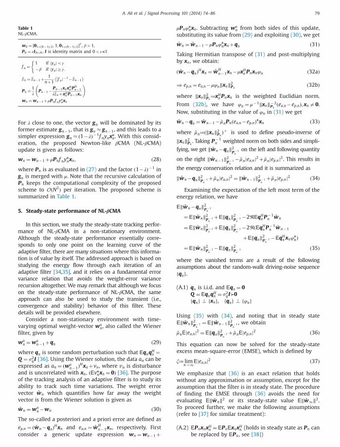
In [28], the βCMA has already been compared andshown to be better than four existing algorithms whichinclude traditional CMA [16] and three of its variants: the(unnormalized) relaxed CMA (RCMA) [40], the Shtrom–Fanalgorithm (SFA) [41] and the generalized CMA (GCMA)[42]. In this work, we provide performance comparison ofNL-βCMA (as summarized in Table 1) with Newton-likeCMA (NL-CMA) [32] and recursive least square CMA (RLS-CMA) [43]. The performances of CMA and βCMA are shownas standard benchmark. Moreover, we consider anunorthodox benchmark [44] which is an adaptive methodfor blind equalization and relies on explicit estimation ofPDF using Parzen window and is termed as a stochasticgradient algorithm (SQD). For reference CMA, βCMA, SQD,RLS-CMA and NL-CMA are summarized in Table 2.

Here we would like to highlight the following importantimplementation details: first, for the SQD scheme therequired compensation factor FðsÞ is computed numerically(see [44] for details). The compensation factor FðsÞ is afunction of the constellation scheme and hence we find thevalues of FðsÞ for 16APSK(8,8) using the bisection method(see Fig. 4). The authors of [44] highlight that the use of asmaller s (e.g., 1) results in an increased number of localminima of the cost function. It is for this reason that we use ahigher value of s (i.e., s¼ 15) in all simulations (thecorresponding FðsÞ is 1.325 as shown in Fig. 4). Secondly,to ensure the stability of NL-CMA, we slightly modify it.According to Miranda et al. [45] one must check thereliability of the error quantity in Hessian. If the statistic oferror quantity in Hessian is not reliable, one must adhere tosimple autocorrelation matrix. Incorporating this recommen-dation and owing to sub-Gaussian nature of the transmittedsignal, the stability of NL-CMA requires to use

zn ¼ ð2jynj2�R2Þ�1 if ð2jynj2�R2Þ�1Z01 otherwise:

(

For simulation purposes, equalizer length is set to

A. Ali et al. / Signal Pr

N¼7 (unless otherwise noted) and w0 ¼ ½01�⌊ðN�1Þ=2c;1;01�⌈ðN�1Þ=2⌉�T i.e., center tap initialization is used. The data

2 We have observed that the traditional root-finding methods likebisection or line-search are good enough for solving (54) and secondly,possibly due to the monotonicity of Nuttall Q-function, the expression(54) yielded unique solutions in all simulation examples considered inthis work.

is modulated using 8APSK(4,4) and 16APSK(8,8) shown inFig. 5(b) and (c). For all experiments, the value of β isobtained using (B.7) (this value is 1.9319 for 8APSK(4,4)

Fig. 4. Numerically computed FðsÞ for 16APSK(8,8).

and 3 for 16APSK(8,8)). ISI (as defined in (2)) is used asindex to evaluate the performance of different equalization

aI

γ aR

1

1.9323

1.586

Fig. 5. (a) A hypothetical dense APSK, (b) practical 8APSK(4,4), and (c) practical 16APSK(8,8).

0 1000 2000 3000 4000 5000 6000 7000−28

−23

−18

−13

−8

ISI [

dB]

Iterations

CMA: μ = 5e−5βCMA: μ =43e−5RLS−CMA μ= 8e−2, λ = 0.98NL−βCMA: μ = 14e−2, λ = 0.98SQD: μ = 18e−5NL−CMA: μ = 65e−3, λ = 0.98

βCMA

NL−CMA

SQDCMA

NL−βCMA

RLS−CMA

h low

A. Ali et al. / Signal Processing 101 (2014) 74–8682

schemes. Experiments comparing the proposed scheme toexisting equalization methods are discussed in 6.1 and 6.2.Furthermore, additional experiments are carried to com-pare the theoretical and practical EMSE of the proposedschemes for both 8APSK(4,4) and 16APSK(8,8). The detailsof these experiments are discussed in 6.3.

6.1. Experiment 1

In this experiment the performance of the proposedscheme is tested for a channel with low eigenvalue spread.The signal is modulated using 16APSK(8,8) and a complex-valued channel with coefficients hR ¼ ½�0:005;0:009;�0:024;0:854; �0:218;0:049; �0:016� and hI ¼ ½�0:004;0:03; �0:104;0:52;0:273; �0:074;0:02�, where h¼ hRþ jhI

is used [46]. The eigenvalue spread of the channel is 5.83.The signal-to-noise ratio (SNR) is set to 30 dB and sta-tionary environment is assumed (i.e., sq ¼ 0, where sq isthe standard deviation of the perturbation qn in (29)).Learning curves are obtained for 7000 iterations and areensemble averaged over 200 independent runs. The step

Fig. 6. Learning curves for channel wit

sizes and forgetting factors of all schemes are adjusted forcomparable performances (i.e., the same steady state ISI)

and are mentioned in Fig. 6. It can be observed from Fig. 6that NL-βCMA shows the fastest convergence rate followedby βCMA.

6.2. Experiment 2

In this experiment, a channel with higher eigenvaluespread is considered. Generally, an increase in the eigen-value spread of the channel results in poor performance ofequalization schemes. For this experiment, the 16APSK(8,8) modulated signal is passed through a channel withimpulse response h¼ ½0;0:1;0:4;0:8;0:4;0:1;0� (the eigen-value spread of this channel is calculated to be 65.28).Again, SNR is set to 30 dB and a stationary environment isassumed. The step sizes and forgetting factors of allschemes are adjusted for comparable performances andare summarized in Fig. 7. The learning curves are obtainedfor 40,000 iterations and are ensemble averaged over 200independent runs. It can be observed from Fig. 7 that theperformance of SQD, CMA and βCMA degrades signifi-cantly in comparison with the first experiment. However,

eigenvalue spread: N¼7, 16APSK(8,8).

it should be noted that NL-CMA, RLS-CMA and NL-βCMAconverge relatively faster. Further, among the three fast

0 0.5 1 1.5 2 2.5 3 3.5 4x 104

−25

−20

−15

−10

−5

0

ISI [

dB]

Iterations

CMA: μ = 1e−4βCMA: μ = 48e−5RLS−CMA μ= 14e−2, λ = 0.98NL−βCMA: μ = 16e−2, λ = 0.98SQD: μ = 33e−5NL−CMA: μ = 12e−2, λ = 0.98

CMA

SQD

βCMANL−CMA

NL−βCMA

RLS−CMA

Fig. 7. Learning curves for channel with high

10−3 10−2 10−1 100−30

−25

−20

−15

−10

−5

0

Stepsize: μ

EM

SE

:ζ [d

B]

SimulationTheory

16APSK(8,8)

8APSK(4,4)

4

A. Ali et al. / Signal Processing 101 (2014) 74–86 83

Fig. 8. Steady state EMSE using 8APSK(4,4) and 16APSK(8,8).

converging schemes, NL-βCMA shows the fastest conver-

gence rate.

6.3. Experiment 3

In this experiment, analytical and empirical perfor-mance of the proposed scheme is compared in a non-stationary environment. In steady state, we assume thatthe proposed scheme converges in the mean to a zeroforcing solution, i.e., the mean of combined channel-equalizer response converges to a delta function witharbitrary delay and phase rotation. We consider a non-stationary channel with sq ¼ 10�3, where sq is the stan-dard deviation of the perturbation qn in (29). The equalizerlength is set to N¼11 and the steady state EMSE isevaluated for 20,000 symbols in a noise-free environment.The forgetting factor is set to 0.98 and step size is varied toobtain the desired curves for both 8APSK(4,4) and 16APSK(8,8). A close match between the analytic and measured

EMSE for both constellation types is observed as depictedin Fig. 8.

7. Conclusion

Exploiting the notion of minimum entropy deconvolu-tion, a cost function was specifically derived for the blindchannel equalization of amplitude phase shift keying signalin digital communication systems. The cost was optimizedadaptively using Newton's method and it yielded a Newton-like constant modulus algorithm NL-βCMA. Tracking analysisof the proposed algorithm was performed based on Sayed-Rupp's feedback approach. Simulation results demonstratedsignificant improvement in performance compared withconventional algorithms. Further, observations of excessmean square error demonstrated good agreement betweentheoretical and practical findings.

Appendix A. Derivation of J ANðynÞ

Consider a continuous APSK signal, where signal alphabetsA¼ aRþ jaI are uniformly distributed (theoretically) over acircular region of radius γ, with the center at the origin. Thejoint PDF of aR and aI is given by (refer to Fig. A1(a))

pA yð Þ ¼1πγ2

;ffiffiffiffiffiffiffiffiffiffiffiffiffiffiffia2Rþa2I

q¼ jynjrγ;

0 otherwise:

8<: ðA:1Þ

Now consider the transformation ~Y ¼ jAj ¼ffiffiffiffiffiffiffiffiffiffiffiffiffiffiffia2Rþa2I

qand

Θ¼∠ðaR; aIÞ, where ~Y is the modulus and ∠ði; jÞ denotesthe angle in the range ð0;2πÞ that is defined by the point (i,j).The joint distribution of the modulus Y and Θ can be obtainedas p ~Y ;Θð ~y; ~θÞ ¼ ~y=ðπγ2Þ; ~yZ0;0r ~θo2π. Since ~Y and Θ are

independent, we obtain p ~Y ð ~y : H0Þ ¼ 2 ~y=γ2; ~yZ0, where H0

denotes the hypothesis that signal is distortion-free. Let~Y1; ~Y2;…; ~YB be a sequence, of size B, obtained by takingmodulus of randomly generated distortion-free signal alpha-bets A, where subscript n indicates discrete time index. Let

eigenvalue spread: N¼7, 16APSK(8,8).

Z1;Z2;…;ZB be the order statistic of sequence f ~Y g. Letp ~Y ð ~y1; ~y2;…; ~yB : H0Þ be a B-variate density of the continuous

−2

0

2

−2−1

01

20

0.2

0.4

0.6

0.8

1

−2

0

2

−2−1

01

20

0.2

0.4

0.6

0.8

1

nse) A

A. Ali et al. / Signal Processing 101 (2014) 74–8684

type, then, under the hypothesis H0, we obtain

pY ~y1;…; ~yB : H0� �¼ 2B

γ2B∏B

k ¼ 1~yk: ðA:2Þ

Next we find scale-invariant PDF psiYð ~y1; ~y2;…; ~yB : H0Þ forgiven B realizations of ~y as follows (below α is some positivescale):

psi~Y ~y1;…; ~yB : H0� �¼Z 1

0p ~Y α ~y1;…; α ~yB : H0� �

αB�1 dα

¼ 2B

γ2B∏B

k ¼ 1~yk

Z Ra=ðzB � z1Þ

0α2B�1 dα

¼ 2B�1

BðzB�z1Þ2B∏B

k ¼ 1~yk; ðA:3Þ

where z1; z2;…; zB are the order statistic of elements~y1; ~y2;…; ~yB, so that z1 ¼minf ~yg and zB ¼maxf ~yg. Nowconsider the next hypothesis (H1) that the signal suffers frommulti-path interference as well as with additive Gaussiannoise (refer to Fig. A1(b)).

Thus, the in-phase and quadrature components of thereceived signal are modeled as normal-distributed; owingto central limit theorem, it is theoretically justified.It means that the modulus of the received signal followsthe Rayleigh distribution,

p ~Y ~y : H1ð Þ ¼ ~ys2~y

exp � ~y2

2s2~y

!; ~yZ0; s ~y 40: ðA:4Þ

The B-variate densities p ~Y ð ~y1;…; ~yB : H1Þ and psi~Y ð ~y1;…; ~yB :

H1Þ are obtained as

p ~Y ~y1;…; ~yB : H1� �¼ 1

s2B~y∏B

k ¼ 1~ykexp � ~y2

k

2s2~y

!; ðA:5aÞ

psi~Y ~y1;…; ~yB : H1� �¼ 1

s2B∏B

~yk

Z 1exp � α2∑B

k0 ¼ 1~y2k0

2s2

!α2B�1 dα:

Fig. A1. PDFs (not to scale) of (a) hypothetical (de

~y k ¼ 1 0 ~y

ðA:5bÞ

Substituting u¼ 12 α

2s�2~y ∑B

k0 ¼ 1~y2k0 , we obtain

psi~Y ~y1;…; ~yB : H1� �¼ 2BΓðBÞ∏B

k ¼ 1~yk

2ð∑Bk ¼ 1

~y2k ÞB

ðA:6Þ

The scale-invariant uniformly most powerful test ofpsi~Y ð ~y1;…; ~yB : H0Þ against psi~Y ð ~y1;…; ~yB : H1Þ provides us,see [20]:

O ~y1� �¼ psi~Y ð ~y1;…; ~yB : H0Þ

psi~Y ð ~y1;…; ~yB : H1Þ¼ 1

B!

∑B

k ¼ 1~y2k

ðzB�z1Þ2

2666437775B

¼ 1B!

∑Bn ¼ 1jynj2

ðmaxfjynjg�minfjynjgÞ2

" #BðA:7Þ

In the present context, where yn is the deconvolvedsequence, we have minfjynjg ¼ 0. Further taking Bth rootof (A.7), ignoring constants and some manipulations, weget (14).

Appendix B. Evaluation of β for APSK

Expressing yn � an�ea;n, note that the amplitude janj isperturbed by ea;n; since ea;n is assumed to be zero-mean(complex-valued) narrowband Gaussian, the modulus jynjbecomes Rician distributed and its PDF (conditioned onjanj) can be expressed as

pðjynj; janjÞ ¼jynjs2

exp � jynj2þjanj22s2

� �I0

jynjjanjs2

� �ðB:1Þ

where s2≔EðR½ea�Þ2 ¼EðI½ea�Þ2, and I0 is zeroth ordermodified Bessel function of first kind (where R½�� and I½��refer to real and imaginary components of the enclosedcomplex-valued entity). Using (B.1), a kth-order momentof modulus jynj can be computed as follows:

Ejynjk ¼ ∑L

j ¼ 1

Mj

M

Z 1

0jynjkpðjynj;RjÞ djynj ðB:2Þ

PSK and (b) Gaussian distributed received signal.

Consider a distortion-free M-symbol complex-valued con-stellation fag which comprises L number of unique moduli,

ocessi

that is janjAfR1;R2;…;RLg, satisfying 0oR1oR2o⋯oRL ¼ γ. Now let Mj be the number of unique symbols onthe j th modulus Rj, this implies Ejanj2 ¼ ð1=MÞ ∑L

j ¼ 1MjR2j

is the per-symbol average energy of constellation fag.

β≔Ejynj2fjynjo γgEjynj2fjynjZ γg

¼Ejynj2�Ejynj2fjyn jZ γg

Ejynj2fjyn jZ γgðB:3Þ

Using (B.1), we obtain Ejynj2 ¼ 2s2þEjanj2 andEjynj2fjyn jZ γg ¼ s2EQ3;0ðjanj=s; γ=sÞ, where Qm;vða; bÞ is theNuttall Q-function as defined below [39]:

Qm;vða; bÞ≔Z 1

bxme�1=2ðx2 þa2ÞIvðaxÞ dx; a; b40 ðB:4Þ

for vZ0;mZ1 and Ivð�Þ is the vth-order modified Besselfunction of first kind. An approximate expression forQ3;0ða; bÞ is given as follows [47]:

Q3;0 a; bð Þ � 2þðaþbÞ2þb2ffiffiffiffiffiffiffiffiffiffiffi8πab

p exp � ðb�aÞ22

!

þ að3þa2Þþbð1þa2Þ4ffiffiffiffiffiffiab

p erfcb�affiffiffi

2p

� �: ðB:5Þ

Exploiting (B.5), we can evaluate β under the limit s-0.Denoting z¼ ðγ�janjÞ=ð

ffiffiffi2

psÞ, note that for γ4 janj, we have

lims-0expð�z2Þ ¼ lims-0erfcðzÞ-0. And for γ ¼ janj, wehave lims-0expð�z2Þ ¼ lims-0erfcðzÞ-1. So it is simpleto show that:

lims-0

Ejynj2fjyn jZ γg ¼ lims-0

s2EQ3;0janjs

;γ

s

� �-

MLγ2

2M: ðB:6Þ

Finally, the asymptotic value of β for the APSK signal underthe condition of vanishing convolutional noise of variance2s2 is given by

lims-0

β-2MEjanj2�MLγ2

MLγ2: ðB:7Þ

References

[1] S. Haykin, Blind Deconvolution, Snewblock Prentice Hall, NewJersey, 1994.

[2] C.R. Johnson Jr., P. Schniter, T.J. Endres, J.D. Behm, D.R. Brown,R.A. Casas, Blind equalization using the constant modulus criterion:a review, Proc. IEEE 86 (10) (1998) 1927–1950.

[3] Z. Ding, Y. Li, Blind Equalization and Identification, Marcel DekkerInc., New York, 2001.

[4] D. Donoho, On minimum entropy deconvolution, in: Proceedings of2nd Applied Time Series Symposium, March 1980, pp. 565–608.

[5] A. Benveniste, M. Goursat, G. Ruget, Robust identification of anonminimum phase system: blind adjustment of a linear equalizerin data communication, IEEE Trans. Autom. Control 25 (3) (1980)385–399.

[6] R.A. Wiggins, Minimum entropy deconvolution, in: Proceedings ofInternational Symposium Computer Aided Seismic Analysis andDiscrimination, 1977.

[7] R.A. Wiggins, Minimum entropy deconvolution, Geoexploration 16(1978) 21–35.

[8] A. Morello, V. Mignone, DVB-S2: the second generation standard forsatellite broad-band services, IEEE Proc. 94 (1) (2006) 210–227.

A. Ali et al. / Signal Pr

[9] R. De Gaudenzi, A. Guillén i Fàbregas, A. Martinez, Turbo-codedAPSK modulations design for satellite broadband communications,Int. J. Satell. Commun. Netw. 24 (4) (2006) 261–281.

[10] C.-Y. Kao, M.-C. Tseng, C.-Y. Chen, The performance analysis ofbackward compatible modulation with higher spectrum efficiencyfor DAB Eureka 147, IEEE Trans. Broadcast. 54 (1) (2008) 62–69.

[11] C. Shaw, M. Rice, Turbo-coded APSK for aeronautical telemetry, IEEEAerosp. Electron. Syst. Mag. 25 (4) (2010) 37–43.

[12] Z. Liu, Q. Xie, K. Peng, Z. Yang, APSK constellation with Graymapping, IEEE Commun. Lett. 15 (12) (2011) 1271–1273.

[13] H. Wang, Y. Li, X. Yi, D. Kong, J. Wu, J. Lin, APSK modulated CO-OFDMsystem with increased tolerance toward fiber nonlinearity, IEEEPhoton. Tech. Lett. 24 (13) (2012) 1085–1087.

[14] S. Fan, H. Wang, Y. Li, W. Du, X. Zhang, J. Wu, J. Lin, Optimal 16-AryAPSK encoded coherent optical OFDM for long-haul transmission,IEEE Photon. Tech. Lett. 25 (13) (2013) 1199–1202.

[15] O. Shalvi, E. Weinstein, New criteria for blind equalization of non-minimum phase systems, IEEE Trans. Inf. Theory 36 (2) (1990)312–321.

[16] D.N. Godard, Self-recovering equalization and carrier tracking intwo-dimensional data communications systems, IEEE Trans. Com-mun. 28 (11) (1980) 1867–1875.

[17] L.R. Litwin, Blind channel equalization, IEEE Potentials 18 (4) (1999)9–12.

[18] J.R. Treichler, B.G. Agee, A new approach to multipath correction ofconstant modulus signals, IEEE Trans. Acoust. Speech Signal Process.31 (2) (1983) 459–471.

[19] R.V. Hogg, More light on the kurtosis and related statistics, J. Am.Stat. Assoc. 67 (338) (1972) 422–424.

[20] Z. Sidak, P.K. Sen, J. Hajek, Theory of Rank Tests, 2 ed. AcademicPress, London, UK, 1999.

[21] J.P. Marques de Sa, L.M.A. Silva, J.M.F. Santos, L.A. Alexandre, Mini-mum Error Entropy Classification, Springer-Verlag, Berlin, Heidel-berg, 2013.

[22] R.C. Geary, Testing for normality, Biometrika 34 (3/4) (1947)S209–S242.

[23] A.T. Walden, Non-Gaussian reflectivity, entropy, and deconvolution,Geophysics 50 (12) (1985) 2862–2888.

[24] M. Ooe, T.J. Ulrych, Minimum entropy deconvolution with anexponential transformation, Geophysical Prospecting 27 (1979)458–473.

[25] W. Gray, Variable norm deconvolution (Ph.D. thesis), Stan. Univ.,1979.

[26] E.H. Satorius, J.J. Mulligan, Minimum entropy deconvolution andblind equalisation, IEEE Electron. Lett. 28 (16) (1992) 1534–1535.

[27] E.H. Satorius, J.J. Mulligan, An alternative methodology for blindequalization, Digital Signal Process.: Rev. J. 3 (3) (1993) 199–209.

[28] S. Abrar, A.K. Nandi, Adaptive minimum entropy equalization algo-rithm, IEEE Commun. Lett. 14 (10) (2010) 966–968.

[29] S. Abrar, A. Zerguine, A.K. Nandi, Adaptive blind channel equaliza-tion, in: C. Palanisamy (Ed.), Digital Communication, InTech Publish-ers, Rijeka, Croatia, 2012, pp. 93–118.

[30] S. Haykin, Adaptive Filtering Theory, Prentice-Hall, Englewood Cliffs,NJ, 1996.

[31] A.K. Nandi, S. Abrar, Adaptive blind equalization based on theminimum entropy principle, in: 5th International Conference onComputers and Devices for Communication (CODEC), December2012.

[32] G. Yan, H.H. Fan, A Newton-like algorithm for complex variableswith applications in blind equalization, IEEE Trans. Signal Process.48 (2) (2000) 553–556.

[33] S. Abrar, A. Zerguine, Enhancing the convergence speed of a multi-modulus blind equalization algorithm, in: IEEE SCONEST, 2004,pp. 41–44.

[34] M. Rupp, A.H. Sayed, A time-domain feedback analysis of filtered-error adaptive gradient algorithms, IEEE Trans. Signal Process. 44 (6)(1996) 1428–1439.

[35] N.R. Yousef, A.H. Sayed, A feedback analysis of the tracking perfor-mance of blind adaptive equalization algorithms, in: IEEE Confer-ence on Decision and Control, vol. 1, 1999, pp. 174–179.

[36] A.H. Sayed, T.Y. Al-Naffouri, Mean-square analysis of normalizedleaky adaptive filters, in: Proceedings of IEEE International Con-ference on Acoustics, Speech and Signal Processing (ICASSP), May2001.

[37] X. Wang, G. Feng, Performance analysis of RLS linearly constrainedconstant modulus algorithm for multiuser detection, Signal Process.89 (2009) 181–186.

[38] A.H. Sayed, Fundamentals of Adaptive Filtering, Wiley-Interscienceand IEEE Press, New York, 2003.

ng 101 (2014) 74–86 85

[39] A.H. Nuttall, Some integrals involving the Q-function, Naval Under-water Systems Center Technical Report 4297, April 1972.

ocessi

[40] O. Tanrikulu, A.G. Constantinides, J.A. Chambers, New normalizedconstant modulus algorithms with relaxation, IEEE Signal Process.Lett. 4 (9) (1997) 256–258.

[41] V. Shtrom, H.H. Fan, New class of zero-forcing cost functions in blindequalization, IEEE Trans. Signal Process. 46 (10) (1998) 2674.

[42] F.R.P. Cavalcanti, A.L. Brandao, J.M.T. Romano, The generalizedconstant modulus algorithm applied to multiuser space-time equal-ization, in: Proceedings of IEEE-SPAWC, 1999, pp. 94–97.

[43] C. Yuxin, T. Le-Ngoc, B. Champagne, X. Changjiang, Recursive least

A. Ali et al. / Signal Pr86

[44] M. Lazaro, I. Santamaria, D. Erdogmus, K.E. Hild, C. Pantaleon,J.C. Principe, Stochastic blind equalization based on PDF fitting usingparzen estimator, IEEE Trans. Signal Process. 53 (2) (2005) 696–704.

[45] M.D. Miranda, M.T.M. Silva, V.H. Nascimento, Avoiding divergence inthe Shalvi–Weinstein algorithm, IEEE Trans. Signal Process. 56 (11)(2008) 5403–5413.

[46] G. Picchi, G. Prati, Blind equalization and carrier recovery using a‘stop-and-go’ decision-directed algorithm, IEEE Trans. Commun. 35(9) (1987) 877–887.

ng 101 (2014) 74–86

squares constant modulus algorithm for blind adaptive array, IEEE [47] S. Abrar, A. Ali, A. Zerguine, A.K. Nandi, Tracking performance of twoconstant modulus equalizers, IEEE Commun. Lett. 17 (5) (2013)

830–833.

Trans. Signal Process. 52 (May (5)) (2004) 1452–1456.