IntroductionPrinciple of Automatic Control

浙江大学控制科学与工程学系

CHAPTER 7CHAPTER 7Frequency Response (P.244, Ch.8)Frequency Response (P.244, Ch.8)

Introduction

2

Outline of Chapter 7

Introduction Bode Plots (Logarithmic plots) Direct Polar Plots Nyquist’s Stability Criterion Phase Margin and Gain Margin and Their

Relation to Stability ………

Introduction

Harry Nyquist (1889-1976)– He received a Ph.D. in physics at

Yale University in 1917.– He developed the Nyquist stability

criterion for feedback systems in the 1930s.

– He worked at AT&T's Department of Development and Research from 1917 to 1934, and continued when it became Bell Telephone Laboratories in that year, until his retirement in 1954.

– http://en.wikipedia.org/wiki/Harry_Nyquist

Frequency Response: 1. Introduction

3

Introduction

Hendrik Wade Bode (1905 –1982)

– an American engineer, researcher, inventor, author and scientist, of Dutch ancestry. As a pioneer of modern control theory and electronic telecommunications

– He received his B.A Degree in 1924,M.A,1926, Ohio State University

– Sponsored by Bell Lab., he successfully completed his Ph.D, in physics in 1935.

– In 1938, he developed his asymptotic phase and magnitude plots.

– http://en.wikipedia.org/wiki/Hendrik_Wade_Bode

Frequency Response: 1. Introduction

4

Introduction

5

Frequency Response: 1. Introduction

The two basic methods for predicting and adjusting a system’s performance: The root-locus methods

Advantage: It displays the location of the closed-loop poles as a parameter (gain) is varied It explicitly gives information about transient performance

The actual time response is easily obtained by means of the inverse Laplace transform because the precise root locations are known.

Disadvantages: It does not provide steady state performance information It cannot handle constraints on frequency ranges for measurement noise and disturbance rejection

Need a new tool to address these issues

Introduction

6

The frequency-response method ---- a good complement to Root Locus We can infer stability and performance, namely steady state performance, from the same plot It is easy to include constraints on frequency ranges Permit evaluation of the effect of noise, exclude the noise by designing a passband and therefore improve the system performance Can use measured data when no model is available (also good forsystem identification) Time delays are handled correctly, contrary to root locus Analysis and design techniques are graphical (asymptotic lines) and easy to use

Frequency Response: 1. Introduction

Introduction

7

In this chapter:

Two graphical representation of transfer functions are presented:

the logarithmic plots

the polar plots.

Developing the Nyquist’s stability criterion using these plots.

The performance of frequency domain.

Frequency Response: 1. Introduction

Introduction

8

Frequency Response1. Introduction: Frequency characteristic

Considering a system

G(s)X(s) Y(s)

System block diagram

)()()( sG

sXsY

))(()( 22

jsjsX

sXsX

tXtx sin)( If the input is

LT

Introduction

9

)())(()(

)()()(

21 nsssssssA

sBsAsG

)()()( sG

sXsY

))(()( 22

jsjsX

sXsX

n

n

n

ssa

ssa

ssa

jsb

jsb

jsjsX

sssssssA

sXsGsY

2

2

1

1

21 ))(()())(()(

)()()(

Frequency Response1. Introduction: Frequency characteristic

Introduction

10

n

n

ssa

ssa

ssa

jsb

jsbsXsGsY

2

2

1

1)()()(

tsn

tststjtj neaeaeaebbety 2121)(

LT-1

For a stable system, all transient components will approach to zero when time t goes infinity, only steady-state response keep down.

t

tjtj

tebbetyty

)(lim)(

Where b can be found by residues theorem or other method.

)()()( sG

sXsY

Frequency Response1. Introduction: Frequency characteristic

Introduction

11

Where G(jω) is a complex number, can be expressed by

jXjGjs

jsjsXsGb js 2

)()())((

)(

jXjGjs

jsjsXsGb js 2

)()())((

)(

)()()( jejGjG

)(Re)(Im)()(

jGjGarctgjG

Similarly, G(-jω): )()( )()()( jj ejGejGjG

tjtj

tebbetyty

)(lim)(

)()()( sG

sXsY

Frequency Response1. Introduction: Frequency characteristic

Introduction

12

)sin()(2

)(

2)(

2)()(

)()(

)()(

tXjGjeeXjG

jXeejG

jXeejGebbety

tjtj

tjj

tjjtjtj

)sin()( tYtyor

Which is the magnitude of steady state response.

Where is usually called

frequency characteristic (----frequency transfer function 3.3).

)()( )()()( jjGj ejGejGjG

There are two methods to obtain G(j): analyzing and experiment.

tXtx sin)(

)()()( sG

sXsY

Frequency Response1. Introduction: Frequency characteristic

Introduction

13

Definition:The frequency response of a system is described as the steady-state

response with a sine-wave forcing function for all values of frequency.

Such as: Input:

Output:

tAtui sin)(

)](sin[)()( tMAtuo

)(M The magnitude ratio of the frequency response

)( The angle of the frequency response

When a linear system with transfer function G(s) is excited by a sinusoid of frequency ω, the steady state output is a sinusoid of the same frequency, with magnitude scaled by |G(jω)| and phase shifted by ∠G(jω).

Frequency Response1. Introduction: Frequency characteristic

Introduction

14

The transfer function of linear and stable system:

)())(()())((

)()()(

21

21

n

m

pspspszszszsK

sAsBsG

)(

)()()()(

)()()(

1

1

jG

pjpjzjzjK

jAjBM

m

m

)()()()(

)()()()(

11 nm pjpjzjzjK

jGjAjB

The frequency response:

jω

jω1

σ

p1

p2

p3 z1

jω1-p1

jω1-p2

jω1-p3jω 1-z 1

See Section.4.12

Frequency Response1. Introduction: Frequency characteristic

Introduction

15

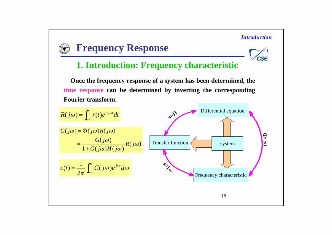
dtetrjR tj )()(

Once the frequency response of a system has been determined, the time response can be determined by inverting the corresponding Fourier transform.

)()()(1

))()()(

jRjHjG

jGjRjjC

(

dejCtc tj)(

21)(

Differential equation

systemTransfer function

Frequency characteristic

s=D

s=jω

jω=D

Frequency Response1. Introduction: Frequency characteristic

Introduction

16

The frequency domain plots belong to two categories:1) The plot of the magnitude of the output-input ratio vs. frequency in

rectangular coordinates and the corresponding phase angle vs. frequency. For example

In logarithmic coordinates these are known as bode plots or log magnitude diagram and phase diagram.

)(:)(: jYoutputjXinput

aja

asa

jXjYjG

)()()(

10.707

a ω→

22)()()(

a

ajXjYM

a ω→0°-45°

-90°

aarctg

jXjY

)()()(

See Section.4.12

Frequency Response1. Introduction: Frequency characteristic

Introduction

17

For a given sinusoidal input signal, the input and steady-state output are of the following forms:

tRtr sin)( )sin()( tCtc

ω

0°

α(ω)

(1)

(3)(2)

ωm

The Frequency-response characteristics of C(jω)/R(jω) in rectangular coordinates

10.707

ωb3

M(ω)(1)

(3)

(2)

ωb2ωm ω

See P.247, Fig.8.1

the closed-loop frequency response is given by

)()()()(1

)()()(

MjHjG

jGjRjC

ideal systemSys.3’s passband

Frequency Response1. Introduction: Frequency characteristic

Introduction

18

0.5 1Re

Im

2) The output-input ratio is plotted in polar coordinates with frequency as a parameter.-----generally used only for the open-loop response and commonly referred to as Nyquist plots.

TssG

11)(

22

2

21)(Im

21)(Re

jGjG

211

11)(

TTj

TjjG

ImG(jω) ω=0

ω=∞

The Nyquist plots is a arc of which the center of the circle is (0.5, j0) and the radius is 0.5

ReG(jω)

Example 7-1: the transfer function is G(s)

Frequency Response1. Introduction: Frequency characteristic

Introduction

19

The log magnitude and the angle are combined into a single curve of log magnitude vs. angle, with frequency as a parameter. This curve is called the Nichols chart or the log magnitude-angle diagram

Example 7-2: the transfer function is G(s)

)1(1)(

Tss

sG)1(

11)1(

1)( 2222 Tj

TT

TjjjG

)90()(0

jTjG

)180(000)(

jjG

ω=∞

Re

Im

ω=0

-T

Frequency Response1. Introduction: Frequency characteristic

Introduction

20

Frequency Response1. Introduction: Frequency characteristic

调入WORD文档－示例之一＿频率响应基本概念

控制科学与工程学系