2013 modele wp tse.doc · In this research, we examine the importance of complementarity among...
44
17‐772 “Complementarity and Bargaining Power” Timothy J. Richards, Celine Bonnet, and Zohra Bouamra‐Mechemache March 2017
Transcript of 2013 modele wp tse.doc · In this research, we examine the importance of complementarity among...

17‐772
“ComplementarityandBargainingPower”
TimothyJ.Richards,CelineBonnet,andZohraBouamra‐Mechemache
March2017
Complementarity and Bargaining Power
Timothy J. Richards, Celine Bonnet, and Zohra Bouamra-Mechemache�
March 1, 2017
Abstract
Bargaining power in vertical channels depends critically on the "disagreement pro�t"or the opportunity cost to each player should negotiations fail. In a multiproduct con-text, disagreement pro�t depends on the degree of substitutability among the productso¤ered by the downstream retailer. Horn and Wolinsky (1988) use this fact to arguefor the clear importance of complementarity relationships on bargaining power. Wedevelop an empirical framework that is able to estimate the e¤ect of retail complemen-tarity on bargaining power, and margins earned by manufacturers and retailers in theFrench soft drink industry. We show that complementarity increases the strength ofretailers�bargaining position, so their share of the total margin increases by almost28% relative to the no-complementarity case.
keywords: bargaining power, complementary goods, Nash-in-Nash equilibrium, retailing,soft drinks, vertical relationshipsJEL Codes: D43, L13, M31
�Richards is Professor and Morrison Chair of Agribusiness, Morrison School of Agribusiness, W. P. CareySchool of Business, Arizona State University; Bonnet and Bouamra-Mechemache are Researchers in theToulouse School of Economics and INRA, Toulouse, France. Contact author: Richards, Address: 7231E Sonoran Arroyo Mall, Mesa, AZ, 85212. Ph. 480-727-1488, email: [email protected] 2016.Users may copy with permission. Financial support from INRA, the Toulouse School of Economics, and theAgricultural and Food Research Initiative (NIFA, USDA) is gratefully acknowledged.
1 Introduction
Empirical models of vertical bargaining power rely critically on estimates of how consumers
respond to changes in prices in the downstream, or consumer, market. Typically, these
models address retail purchases from only one category at a time (Villas-Boas and Zhao
2005; Villas-Boas 2007), whereas consumers tend to buy products by the shopping basket
(Manchanda, Ansari, and Gupta 1999; Kwak, Duvvuri, and Russell 2015). Within a single
category, the choices �di¤erent brands, for example �are plausibly all substitutes for each
other. When buying multiple categories at a time, however, the purchase is likely to consist
of a mix of substitutes and complements. In a theoretical treatment of this setting, Horn
and Wolinksy (1988) show that when wholesale prices are negotiated between suppliers and
downstream buyers, di¤erences in how consumers respond to price changes can alter the
nature of the bargaining outcome qualitatively for the upstream �rms. While the potential
for a complex pattern of substitutability and complementarity among items in the shop-
ping basket may be relatively inconsequential if the items are from di¤erent manufacturers,
the implications for vertical relationships between retailers and manufacturers cannot be ig-
nored. In this research, we examine the importance of complementarity among retail grocery
products for bargaining power between retailers and manufacturers.
With the global consolidation of food production in fewer and fewer hands, some manu-
facturers may be responsible for items in several categories in a typical shopping basket. We
argue that this observation may have important implications for the balance of bargaining
power between manufacturers and retailers in the food supply chain. Namely, when down-
stream �rms sell complementary goods, an upstream supplier has less bargaining power than
if products downstream are substitutes because the cost of not arriving at an agreement is
higher for the supplier. Why? Because retailers are interested in category sales and manu-
facturers are interested in selling only their brands. When a retailer cannot sell a particular
brand, it will sell another, while if a manufacturer selling to multiple retailers loses a distrib-
ution contract, the lost sales cannot be replaced as easily. If the manufacturer sells items in
1
substitute categories �ketchup and mustard, for instance �the e¤ect may not be substantial
as lost sales can be regained elsewhere. However, if the manufacturer sells complementary
goods �potato chips and dip, for instance �the e¤ect of losing sales from a dropped brand
in one category will be ampli�ed by losses in the other. Therefore, the opportunity cost of
arriving at an agreement, which is manifest in the di¤erence between the current and dis-
agreement pro�ts, is higher for the manufacturer than the retailer. Because retail bargaining
power is the mirror of manufacturer power, we expect retailer bargaining power to be higher
when goods are complements.
It is well understood that complementarity a¤ects pricing strategies among retailers
downstream. Rhodes (2015) and Smith and Thomassen (2012) argue that internalizing cross-
product pricing e¤ects on the intra-retailer margin with complementarity leads to lower retail
prices as retailers have an incentive to drive volume rather than margin. On the other hand,
Richards and Hamilton (2016) show that complementarity on the inter-retailer margin is
associated with anti-competitive e¤ects and is a source of market power for retailers. How-
ever, none of these studies focus on vertical relationships between multi-product retailers
and manufacturers.
The increasing prevalence of highly granular data on consumer purchases, whether from
frequent shopper cards or from household panel data sets, both highlights the importance
of examining shopping-basket purchases, and makes structural models of multi-product pur-
chasing behavior possible. By observing purchases on each shopping-occasion basis, we have
a better understanding of how consumers combine products in a shopping list. Namely, pre-
vious research shows that consumers tend to make multiple discrete purchases (Dube 2004,
2005; Richards, Pofahl, and Gomez 2012) and tend to purchase some pairs of products at
the same time, for reasons other than traditional price-based complementarity reasons (Song
and Chintagunta 2007; Mehta 2007). In this paper, we develop a new model of retail demand
that explicitly recognizes the importance of these two features of consumer-level purchase
behavior.
2
Our demand model is of the multi-variate logit (MVL) class, in which consumers are
assumed to make discrete choices among baskets of items. Because each item can reside in
one of many di¤erent baskets, the choices cannot be described by a traditional logit model.
Russell and Peterson (2000) show how the auto-logistical model from spatial econometrics
(Besag 1974) can be used in a shopping-basket model environment to consistently estimate
demand elasticities that include a full-range of possibilities, from complementarity to substi-
tutability, and independence in demand. Further, because the estimating model assumes a
closed-form, Kwak, Duvvuri, and Russell (2015) show that it can be used to inform a wide
range of practical issues in structural demand modeling. For this paper, we demonstrate
how the implicit assumption of strict-substitutability from more usual logit models of de-
mand can impart signi�cant bias to bargaining power estimates in an environment in which
demand relationships are likely to be more general.
Structural models of vertical relationships between retailers and manufacturers are, by
now, reasonably well understood. Assuming Bertrand-Nash rivalry among downstream re-
tailers, the solution to the Nash bargaining problem between retailers and manufacturers
yields a single parameter that describes the share of the total margin that is appropriated by
either the manufacturer or the retailer, depending on the relative bargaining strength of ei-
ther party (Draganska, Klapper, and Villas-Boas 2010).1 While others investigate structural
factors that may in�uence the degree of bargaining power possessed by either side (Meza
and Sudhir 2010; Haucap et al. 2013; Bonnet and Bouamra-Mechemache 2016), the role
of demand-interrelationships among downstream retailers is not well understood, despite
the clear theoretical importance it plays in the likely outcome of any negotiation (Bulow
et al. 1985; Binmore, Rubinstein and Wolinsky 1986; Horn and Wolinsky 1988).2 In this
paper, we show that the structure of demand, namely whether products are substitutes or
1Misra and Mohanty (2006) develop a similar approach to modeling vertical relationships in which pricesare the result of a Nash bargaining equilibrium, and show that their model �ts the data better than existingempirical models in two di¤erent grocery categories.
2Iyer and Villas-Boas (2003) and Feng and Lu (2013a,b) apply a Nash bargaining model to verticalrelationships in a supply-chain context.
3

complements, can have dramatic e¤ects on estimated bargaining-power parameters.3
We test our hypothesis using data on multi-category soft drink purchases among house-
holds in France. While a discrete-choice model of category incidence would restrict all pairs
of categories to be substitutes, we �nd that complementarity is more common than subti-
tutability at the brand level. When we condition equilibrium wholesale prices on our MVL
demand estimates, we �nd that complementarity is associated with less manufacturer bar-
gaining power and greater retail bargaining power. When products sold by one manufacturer
are complements downstream, the disagreement pro�t, which is the amount earned if the
parties fail to agree, is lower with complementarity than under strict substitutability. Lower
disagreement pro�t implies a higher opportunity cost of agreeing. As a result, manufactur-
ers are essentially more keen to arrive at a negotiated solution, so their bargaining power is
lower. Our �ndings have broader implications for vertical relationships in any other indus-
try in which powerful suppliers sell complementary products through oligopoly downstream
retailers.
Our research contributes to both the theoretical literature on vertical relationships be-
tween suppliers and retailers, and the empirical literature on the nature of bargaining power
in those relationships. While Horn and Wolinsky (1988) identify the mechanism that is
likely to in�uence bargaining power in vertical relationships when products interact in the
downstream market, their model is highly stylized, as it is framed in terms of an upstream
duopoly and downstream duopoly �rms. Our model, however, is able to accommodate more
general oligopoly relationships among �rms both upstream and downstream. In terms of the
empirical bargaining power literature, we show how the single-category model of Draganska,
Klapper, and Villas-Boas (2010) can be extended to a more general, multi-category demand
framework, and show that doing so can have dramatic e¤ects on the nature of the equilibrium
bargaining solution that results.
In the next section, we describe our multi-category demand model, and how it is able to
3Dukes, Gal-Or, and Srinivasan (2006) show that di¤erences among retailers can be important in in�u-encing bargaining power in the vertical channel. Our empirical model captures retailer heterogeneity.
4

capture complementarity in household-level beverage purchases. The Nash bargaining power
model is presented in the third section, where we show how our core hypotheses regarding
complementarity and bargaining power are tested. We describe the data from our French
soft-drink example in the fourth section, and present some stylized facts that suggest how
a shopping-basket approach is both appropriate and necessary in data such as ours. We
present and interpret the demand and pricing model results in a �fth section, while the
�nal section concludes, and o¤ers some implications for settings beyond our retail grocery
example.
2 Empirical Model of Multi-Category Pricing
2.1 Overview
We examine the role of complementarity in bargaining power using a structural model of
multi-category retail demand, and vertical pricing relationships between beverage manu-
facturers and retailers in France. Our model is innovative in that the demand component
describes relationships among beverages found in a typical shopping-basket, unlike most
conventional analyses in this area (Draganska, Klapper, and Villas-Boas 2010). Our demand
model is multi-category in nature in that it recognizes the fact that items are purchased
through a discrete-choice data generating process, but will nearly as often be complemen-
tary as they are substitutes with other items in the basket. When a retailer sells items from
the same manufacturer that are likely to be complements, the implications for bargaining
power in the vertical channel may be dramatic. Our model is structural in that we estimate
equilibrium pricing relationships in the vertical channel, conditional on the structure of re-
tail demand (Villas Boas 2007; Bonnet and Dubois 2010; Bonnet and Bouamra-Mechemache
2016) across multiple product categories.
5

2.2 Model of Multi-Category Demand
We develop our empirical model of multi-category choice and local-content demand from
a single utility function, in the sense that consumers are assumed to maximize utility in
choosing which categories to buy from on each trip to each store, r = 1; 2; :::; R. For clarity,
we suppress the store subscript until we describe the equilibrium vertical pricing game below.
Consumers h = 1; 2; 3; :::; H in our model select items from among i = 1; 2; 3; :::; I categories,
ciht; in assembling a shopping basket, or bundle, bht = (c1ht; c2ht; c3ht; :::; cIht) on each trip,
t. De�ne the set of all possible bundles bht 2 B and the set of categories i; j 2 I: We focus
on purchase incidence, or the probability of choosing items from a particular category on
each trip to the store, and regard the brand of the chosen item as an attribute of the choice.
We assume consumers purchase only one brand within each category in order to remain
consistent with the literature. We further assume consumers choose categories in order
to maximize utility, Uht; and follow Song and Chintagunta (2006) in writing their utility in
terms of a discrete, second-order Taylor series approximation to an arbitrary utility function.
Utility is written as:
Uht(bht) = Vht(bht) + "ht (1)
=Xi2I�ihtciht +
Xi2I
Xj2I�ijhcihtcjht + "ht;
where �iht is the baseline utility for category i earned by household h on shopping trip t , ciht
is a discrete indicator that equals 1 when category i is purchased, and is 0 otherwise, "ht is
an error term that is Gumbel distributed, and iid across households and shopping trips, and
�ijh is a household-speci�c parameter that captures the degree of interdependence in demand
between categories i and j, such that if �ijh < 0; the categories are substitutes, if �ijh > 0,
the categories are complementary, and if �ijh = 0; the pair of categories are independent in
demand. For example, we would expect to �nd �ijh > 0 for ketchup and hamburger, but
�ijh < 0 for ketchup and bbq sauce, and �ijh = 0 for ketchup and laundry detergent. In order
to ensure that the model is identi�ed, it is necessary that all �ii = 0 and that symmetry be
6

imposed on the matrix of cross-purchase e¤ects such that �ijh = �jih;8i; j; h (Besag 1974,
Cressie 1993, Russell and Petersen 2000).
The probability that a household purchases in a given category on a purchase occasion,
or category incidence, depends on both perceived need, and marketing activities from the
brands in the category (Bucklin and Lattin 1992, Russell and Petersen 2000). Because
we seek to examine demand relationships, and pricing behavior, at the brand-and-retailer
level, however, we extend the usual MVL speci�cation to consider the demand for speci�c
items within each category. We then capture interactions in a parsimonious way through
the interaction terms given in (1).4 Therefore, we write baseline utility for each brand (k),
retailer (r), and category (i) as:
�ikrht = �ikr + �ihXikr + iZh; (2)
where �ikr are �xed e¤ects that control for the particular brand, k; that is purchased from
retailer, r, in category i, Xik is a matrix of category-speci�c marketing mix elements for each
brand, and Zh is a matrix of household attributes.5 Household attributes a¤ect perceived
need, as measured by the rate at which a household consumes products in the category,
which when combined with the frequency of category-purchase, determines the amount on
hand (INVh). We infer household inventory using methods that are standard in this lit-
erature (Bucklin and Lattin 1992). Namely, we calculate the category-consumption rate
for each household by calculating their total purchases over the sample period, and divide
by the total number of days in the data set. We then initialize inventory at the average
consumption-rate at the start of the time-period for each household, and increment inven-
tory upward with purchases, and downward each day by the average consumption rate. Need
is also determined by more fundamental household factors such as the size of the household
(HHh), income level (INCh), and education (EDUh). Any state dependence in demand
4Conceptually, a fully-nested version of the MVL would be preferably, but proved to be empiricallyintractable.
5One brand each in the fruit juice and iced tea categories was o¤ered in only one retailer, so brand e¤ectscould not be identi�ed separately from retailer e¤ects.
7

is assumed to be captured by the inventory variable as it re�ects intertemporal changes in
consumption behavior. Marketing mix elements at the brand-category level include the price
of the individual items in each category (pikr), and an indicator of whether the item was on
promotion during the purchase occasion at a particular retailer (PRikr).6
Each of the variables entering (2) represent sources of observed heterogeneity, whether at
the item (brand / category / retailer) (Xikr) or household (Zh) levels. However, there is also
likely to be substantial unobserved heterogeneity in household preferences and in attributes
of the item that may a¤ect incidence. Therefore, we capture unobserved heterogeneity in
item preference by allowing for randomly-distributed category-interactions (�ijh) and item-
level price-response (�pih). Formally, therefore, we estimate:
�pih = �pi0 + �pi1�i1; vi1 � N(0; �1); 8i; (3)
�ijh = �ij0 + �ij1�2; v2 � N(0; �2);
for the price-element of the marketing-mix matrix, and for each of the ij category-interaction
parameters. By allowing for a general pattern of correlation among these parameters (Singh,
Hansen, and Gupta 2005), we capture a primary source of coincident demand among cate-
gories. In other words, if households tend to be correlated in terms of their price sensitivity,
then allowing for co-movements in demand due to price responsiveness will remove some ele-
ment of randomness from the error term, leaving less variation to be explained by other fac-
tors. This extension to the MVL model, by incorporating random parameters into both the
marketing-mix and category-interaction parameters is called the random-parameters MVL
model, or RP-MVL.
With the error assumption in equation (1), the conditional probability of purchasing in
each category assumes a relatively simple logit form. Following Kwak, Duvvuri, and Russell
(2015), we simplify the expression for the conditional incidence probability by writing the
cross-category purchase e¤ect in matrix form, where: �h = [�1h;�2h; :::;�Nh] and each �ih6The promotion indicator is inferred from the prices paid by each household. If the price paid is less
than 90% of the previous price paid for that item, and the price rises back to the previous level on the nextpurchase occasion, then we infer that the purchase was made on promotion.
8

represents a column vector of the I � I cross-e¤ect �h matrix which is de�ned as:
�h =
266666640 �12h �13h ::: �1Ih�21h 0 ::: �2Ih�31h �32h 0 ::: �3Ih: : : ::: :: : : ::: :�I1h �I2h �I3h ::: 0
37777775 ; (4)
so that the conditional utility of purchasing an item in category i is written as:
Uht(cikrhtjcjkrht) = �0htbht +�0ihbht + "ht; (5)
for the items i; k; r in the basket vector bht: Conditional utility functions of this type po-
tentially convey important information, and are more empirically tractable that the full
probability distribution of all potential assortments (Moon and Russell 2008), but are lim-
ited in that they cannot describe the entire matrix of substitute relationships in a consistent
way, and are not econometrically e¢ cient in that they fail to exploit the cross-equation re-
lationships implied by the utility maximization problem. To see this more clearly, we derive
the estimating equation implied by the Gumbel error-distribution assumption, conditional
on the purchases made in all other categories, cjht: With this conditional assumption, the
probability of purchasing an item from category i = 1 is written as:
Pr(c1krht = 1jcjkrht) =[exp(�1krht +�
01hbht)]
c1krht
1 + exp(�1krht +�01hbht); (6)
and bht represents the basket vector. Estimating all I of these equations together in a system
is one option, or Besag (1974) describes how the full distribution of bht choices are estimated
together.
Assuming the �h matrix is fully symmetric, and the main diagonal consists entirely of
zeros, then Besag (1974) shows that the probability of choosing the entire vector bht is
written as:
Pr(bht) =exp(�0htbht +
12b0ht�hbht)X
bht2B
[exp(�0htbht +12b0ht�hbht)]
; (7)
9

where Pr(bht) is interpreted as the joint probability of choosing the observed combination
of categories from among the 2I potentially available from I categories.7 Assuming the
elements of the main diagonal of � is necessary for identi�cation, while the symmetry as-
sumption is required to ensure that (7) truly represents a joint distribution, a multi-variate
logistic distribution, of the category-purchase events. Essentially, the model in (7) represents
the probability of observing the simultaneous occurrence of I discrete events �a shopping
basket �at one point in time. And, due to the iid assumption of the logit errors associated
with each basket choice, the model in (7) implicitly assumes that the baskets are subject
to the independence of irrelevant alternatives (IAA), but the categories within the basket
are allowed to assume a more general correlation structure (Kwak, Duvvuri, and Russell
2015). Aggregating (7) over households then produces an expression for the probability of
purchasing each basket, and each component brand, category, retailer combination captured
by each basket.
Given the similarity of the choice probabilities to logit-choice probabilities, it is perhaps
not surprising that the form of the elasticity matrix is also similar. Given the probability
expression above, the marginal e¤ect of a price change in brand k, category i; and retailer
r, on the own-probability of purchase is written as:
@ Pr(cikr)
@pikr= �pih Pr(cikr)(1� Pr(cikr)); (8)
where �pih is the household-speci�c marginal utility of income for an item in category i,
and Pr(cikr) includes all baskets that contain the speci�c i; k; r item: Similarly, the marginal
e¤ect of a change in the price of an item in a di¤erent category (j), of a di¤erent brand (l)
in the same store on the probability of purchasing an item in category i, when the items are
7The practical limitations of describing 2I choices are somewhat obvious. Recently, others have developedways to either reduce the dimensionality of the bht vector, or of estimating it more e¢ ciently. Kwak,Duvvuri, and Russell (2015) focus on "clusters" of items within conventional category de�nitions, whileMoon and Russel (2008) project the bht vector into household-attribute space, so only 2 parameters areestimated. Kamakura and Kwak (2012) use the random-sampling approach of McFadden (1978) to reducethe estimation burden while leaving the size of the problem intact. Because our problem is well-describedwith only a small number of categories (4), we estimate the MVL model in its native form.
10

in the same baskets is given by:
@ Pr(cikr)
@pjlr= ��pih Pr(cikr) Pr(cjlr); (9)
and the marginal e¤ect of change in the price of an item that may be in the same category,
and of the same brand, but in a di¤erent store is:
@ Pr(cikr)
@piks= ��pih Pr(cikr) Pr(ciks) (10)
for all products not in the same store. With these expressions, we can estimate an entire
matrix of price responses, for all items with respect to all other items, whether they are from
the same brand, category, and store, or if they di¤er entirely.
In the absence of unobserved heterogeneity, the MVL model is estimated using maximum
likelihood in a relatively standard way. However, because we allow a range of parameters to
vary across panel observations, the likelihood function no longer has a closed form. Therefore,
the model is estimated using simulated maximum likelihood (SML, Train 2003), using r =
1; 2; 3::::R simulations. De�ne a set of indicator variables zk that assume a value of 1 if basket
k is chosen and 0 otherwise, so the likelihood function for a panel over h cross-sections and
t shopping occasions per household yields a simulated likelihood function written as (Kwak,
Duvvuri, and Russel 2015):
Lh(bht) =1
R
RXr=1
Yt
Yk
(Pr(bht = bkht)
zk ; (11)
where the joint distribution function for all possible baskets is given in (7). We then take
the log of (11), sum over all households, and maximize with respect to all parameters:
LLF (�;�; ;�) =PH
h=1 log Lh(bht): To increase the e¢ ciency of the SML routine, the
simulated draws follow a Halton sequence with 50 draws.
The MVL is powerful in its ability to estimate both substitute and complimentary rela-
tionships in a relatively parsimonious way, but su¤ers from the curse of dimensionality. That
is, with N products, the number of baskets is N2 � 1, so the problem quickly becomes in-
tractable for anything more then a highly stylized description of the typical shopping basket.
11
Therefore, we restrict our attention to four categories that are likely to exhibit a pattern
of both substitute and complementary relationships. Other methods have been developed
in order to explicitly address the problem of dimensionality inherent in shopping-basket de-
mand estimation (Kamakura and Kwak 2012), but have not yet proven to be as amenable
to estimation in panel-scanner data as the RP-MVL.
To this point, the development of the MVL model is relatively standard. However, in our
application we are interested not only in the magnitude of each of the �ij parameters (drop-
ping the household subscripts for clarity), but how a consumer�s willingness to substitute
(or complement) between categories a¤ects equilibrium prices charged by retailers in each
category, and how the resulting margins are divided between retailers and manufacturers.
We use the parameter estimates from the RP-MVL model above to condition equilibrium
pricing behavior by retailers, and their bargaining power relative to manufacturers in the
vertical channel using the Nash bargaining model developed in the next section.
3 Bargaining Power Model
In this section, we describe the empirical model used to estimate the e¤ect of complementarity
on brand-level bargaining power. For this purpose, we use the vertical Nash-in-Nash model
developed by Misra and Mohandy (2006) and Draganska, Klapper, and Villas-Boas (2010).
Our model di¤ers from either of these studies, however, in that we explicitly account for the
e¤ect of complementarity. Horn and Wolitzky (1988) show that complementarity is likely
to be critical in in�uencing the level of bargaining power possessed by either side because
downstream-substitution patterns a¤ect the disagreement pro�t earned by each party should
negotiations fail. Disagreement pro�t, in turn, depends upon how much the market share
of each product would rise if the object of the negotiation is dropped from the product line-
up. With strict-substitute demand models, the notion that market share will rise if another
product is dropped is a given as it is enforced, mathematically.
With complementary products, however, the e¤ect is not as straightforward. If I am a
12
retailer, and negotiations fail with my pasta-sauce supplier, I will still sell pasta-sauce from
another supplier (substitute product). If I also sell pasta from this same pasta-sauce supplier
(a complementary product), then the supplier�s loss in sales is magni�ed by the complemen-
tary relationship between pasta and sauce, but I continue to sell pasta from another supplier.
The disagreement pro�t for the retailer, therefore, is higher in the complementarity case than
it is when products are constrained to be strict substitutes, so retailer bargaining power is
expected to be higher. Ultimately, however, the complexity of the relationships involved in
any given shopping basket means that the implications of complementarity for bargaining
power is an empirical question. In this section, we describe how the Nash-in-Nash bargaining
power model applies to the case of shopping-basket shoppers.
We characterize the marketing channel as consisting of several, multi-product retailers,
and our several, multiple-product suppliers that sell to each of our sample retailers. We
assume retailers arrive at a Nash equilibrium in horizontal competition, pricing as if they were
Bertrand-Nash competitors selling di¤erentiated products. Following recent developments
in the empirical literature on vertical relationships, we then assume the supplier achieves a
Nash bargaining solution (Horn and Wolinsky 1988) with each of the retailers independently,
and estimate the resulting bargaining power parameter that divides the total margin (from
marginal production cost to retail price) between the supplier and retailers according to
their relative negotiating abilities (Draganska, Klapper, and Villas-Boas 2010). We begin by
solving for the optimal margin values, and then solve for the Nash bargaining solution.
Beginning with the retailer decision, and suppressing time period index (t) for clarity,
retailer g sets a price for each item under a maintained assumption of Nash rivalry to solve
the following problem: �g = maxpjPJg
j=1(pj � crj � wj)Msj; g = 1; 2; :::; G; where M is
total market demand, wj is the wholesale price, crj are unit retailing costs, sj is the market
share de�ned above, and retailer g sells a total of Jg products. Marginal retailing costs are
assumed to be constant in volume, and a function of input prices, which is plausible given the
share of store-sales accounted for by any individual product. The solution to this problem
13
is written in matrix notation as: mg= p� cr�w = �(g � sp)�1s; where mg is a vector of
retail margins, p is a J � 1 vector of prices, w is a J � 1 vector of wholesale prices, cr is a
J � 1vector of retailing costs (estimated as a linear function of retailing input prices), s is a
J � 1 vector of market shares, sp is a J � J matrix of share-derivatives with respect to all
retail prices, g is a retail ownership matrix, with each element equal to 1 if the row item
and column item are sold by the same retailer, and 0 otherwise, and � indicates element-
by-element multiplication. Equilibrium retail prices, therefore, are determined by demand
interrelationships at the retail level in Bertrand-Nash rivalry.
If retail prices are assumed to be determined by the Bertrand-Nash game played among
retailers, and marginal production costs determined by the engineering relationships that
govern the cost of making each item, then the allocation of the total margin (from retail
prices to marginal production costs) depends on how the wholesale price (wj) is determined.
Wholesale prices, in turn, are assumed to be determined by a Nash bargaining process
(Horn and Wolinksy 1988; Draganska, Klapper, and Villas-Boas 2010). In a Nash bargaining
solution, the allocation of the total margin between wholesalers and retailers depends on two
elements: (1) the disagreement pro�t that results when negotiations fail and the product
is not sold, and (2) the bargaining power parameter, which is a function of the inherent
bargaining position of the two players. The disagreement pro�t term re�ects the fact that
if a product is not sold, the sales, and pro�ts, of all the other items sold by the retailer,
or manufacturer, are a¤ected by the nature of the demand interrelationships each face.
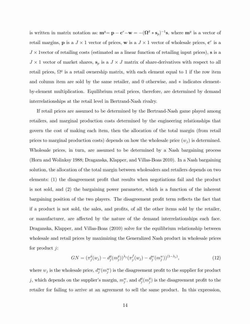
Draganska, Klapper, and Villas-Boas (2010) solve for the equilibrium relationship between
wholesale and retail prices by maximizing the Generalized Nash product in wholesale prices
for product j:
GN = (�gj (wj)� dgj (m
gj ))
�j(�fj (wj)� dwj (mwj ))
(1��j); (12)
where wj is the wholesale price, dwj (mwj ) is the disagreement pro�t to the supplier for product
j, which depends on the supplier�s margin, mwj ; and d
gj (m
gj ) is the disagreement pro�t to the
retailer for failing to arrive at an agreement to sell the same product. In this expression,
14

�j is the bargaining power parameter, which allocates the share of pro�t to the retailer
(�j) and the wholesaler (1 � �j) from the trade of product j. The �rst-order condition to
maximizing the Generalized Nash product is (dropping the product subscript and arguments
of the disagreement pro�t):
@GN
@w= �(�g � dg)(��1)@�
g
@w(�f � df )(1��) + (1� �)(�g � dg)�(�f � df )��@�
f
@w= 0: (13)
This expression simpli�es to give the equilibrium relationship between retail and wholesale
prices as a function of their respective disagreement pro�ts, and the relative bargaining power
parameter:
�
�(�f � df )@�
g
@w
�+ (1� �)
�(�g � dg)@�
f
@w
�= 0: (14)
Because retail prices are assumed �xed at the BN solution, the derivatives @�g
@w= @�f
@w=Ms
so this simpli�es to: (�g � dg) =�1���
�(�f � df ): Stacking over all item-pro�ts provides a
simple solution in matrix notation that de�nes the equilibrium bargaining power parameter,
and the margins for each item:
mf =
�1� ��
�[f � S]�1[g � S]mg; (15)
where f is the J�J manufacturer ownership matrix (with element = 1 if the manufacturer
owns product j and zero otherwise), mf is the manufacturer margin, and S is the matrix
that de�nes the incremental pro�t between when a product is sold, and when it is not (see
Draganska, Klapper, and Villas-Boas 2010 for details on its construction). Substituting the
expression for retail margins (mg) above, and solving for the total margin gives:
p� cf � cr = ��1� ��
[f � S]�1[g � S] + I�[g � sp]�1s(p); (16)
for the �nal estimating equation, where cf is a vector of manufacturing costs, estimated as
a linear function of manufacturing input prices.
In our empirical application, we recognize that bargaining power is likely to vary by each
retailer-manufacturer dyad in the data. Therefore, we allow the � parameter to be randomly
15

distributed over the entire category-retailer-brand sample (�j = �j0 + �j1�3; v3 � N(0; �3))
so that bargaining power re�ects any factors that may in�uence the relative strength of
each player�s position. Importantly, however, allowing � to vary randomly also means that
we are able to recover a value for the bargaining power parameter for every observation in
the data set. In this way, we use a supplementary regression to test whether bargaining
power is higher or lower for products that are complements for other products. Determining
whether an item is a complement or substitute is not straightforward because the notion
of complementarity is de�ned dyad-by-dyad, yet we seek a summary measure for each item
in our data set. Therefore, we use the matrix S to determine whether each product is a
net complement or net substitute over all other items in the store. That is, if removing the
item from the product lineup reduces the demand for all other products, then it must be
primarily a complement, and vice versa. We then de�ne a variable measuring the extent
of the impact of removing each item on the demand for all other items (COMPj) that
captures the complementary (COMPj < 0) or substitute (COMPj > 0) status of the item
in question.
Given that the bargaining power estimation routine already controls for the identity of
the retailer and other factors, we test our core hypothesis using a straightforward regression
model in which bargaining power is estimated as a linear function of the complementarity
variable, and an interaction term between complementarity and time such that:
^
�j = �0 + �1COMPj + �2COMPj � t+ �; (17)
where^
�jis the �tted-value from the random-parameter function described above, � is an iid
random variable, COMP � t is the complementarity variable interacted with a time variable,
and �i are parameters to be estimated.
In this model, our maintained hypothesis is supported if �1 < 0, as this implies that
retailers tend to have more bargaining power for complementary products than they do for
substitute products (recall that the COMP variable is negative-valued as it is measured as
the e¤ect on other product shares if the product is removed), and manufacturers, of course,
16
have less. Based on the theoretical insight of Horn and Wolinsky (1988), we attribute
this outcome to the exercise of market power in allocating the transaction surplus between
the buyer and the seller due to the fact that goods are complements. When retailers sell
complementary goods, and manufacturers are able to internalize the e¤ects of selling their
products through multiple retailers, then manufacturers�bargaining power will be lower for
that set of complementary items. Similarly, if �1 > 0 then suppliers earn higher margins
on complementary products, as the degree of bargaining power shifts to suppliers when
products are complements, contrary to the Horn and Wolinsky (1988) model. Further, if
�2 < 0 then any complementarity-premium earned by retailers erodes over time, and, by
de�nition, suppliers bene�t over time.
4 Data and Identi�cation Strategy
In this section, we describe the French soft-drink data and how we identify the parameters of
both the demand model, and the bargaining power model. Our data are from a large-scale
French consumer panel maintained by Kantar TNS Worldpanel for the year 2013. The panel
is designed to be representative of all French households, so contains observations from all
regions, urban and rural, and draw households from across all socioeconomic strata. We
draw a random sample of 330 households from the panel, who recorded a total of 29,026
transactions in 2013. As a household panel, the Kantar data includes information on the
speci�c item that was purchased, the package attributes, howmuch was paid, where and when
it was purchased, and a large set of household socioeconomic and demographic attributes.
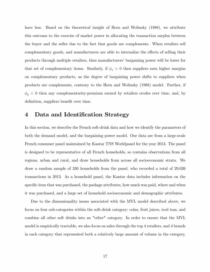
Due to the dimensionality issues associated with the MVL model described above, we
focus on four sub-categories within the soft-drink category: colas, fruit juices, iced teas, and
combine all other soft drinks into an "other" category. In order to ensure that the MVL
model is empirically tractable, we also focus on sales through the top 4 retailers, and 4 brands
in each category that represented both a relatively large amount of volume in the category,
17
and a presence in as many retailers as possible.8 Focusing on as many of the same brands
across retailers as possible is desirable for identi�cation as we capture as much cross-sectional
variation in margin behavior as possible. Although this 4 � 4 � 4 design may seem more
restrictive than is normally the case in other shopping-basket demand models, it is necessary
in our case because we need to be able to isolate speci�c retail-manufacturer pairs from the
demand model through the bargaining-power estimation process.
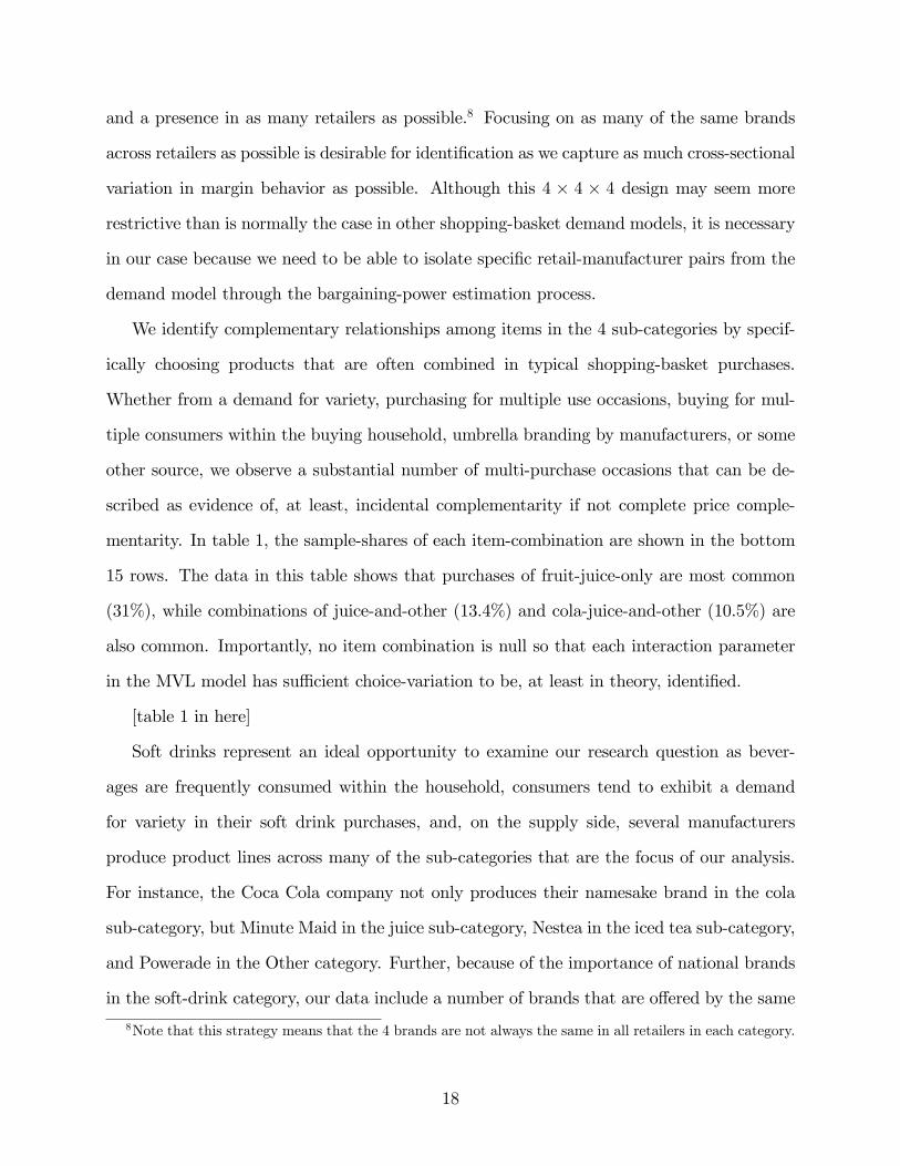
We identify complementary relationships among items in the 4 sub-categories by specif-
ically choosing products that are often combined in typical shopping-basket purchases.
Whether from a demand for variety, purchasing for multiple use occasions, buying for mul-
tiple consumers within the buying household, umbrella branding by manufacturers, or some
other source, we observe a substantial number of multi-purchase occasions that can be de-
scribed as evidence of, at least, incidental complementarity if not complete price comple-
mentarity. In table 1, the sample-shares of each item-combination are shown in the bottom
15 rows. The data in this table shows that purchases of fruit-juice-only are most common
(31%), while combinations of juice-and-other (13.4%) and cola-juice-and-other (10.5%) are
also common. Importantly, no item combination is null so that each interaction parameter
in the MVL model has su¢ cient choice-variation to be, at least in theory, identi�ed.
[table 1 in here]
Soft drinks represent an ideal opportunity to examine our research question as bever-
ages are frequently consumed within the household, consumers tend to exhibit a demand
for variety in their soft drink purchases, and, on the supply side, several manufacturers
produce product lines across many of the sub-categories that are the focus of our analysis.
For instance, the Coca Cola company not only produces their namesake brand in the cola
sub-category, but Minute Maid in the juice sub-category, Nestea in the iced tea sub-category,
and Powerade in the Other category. Further, because of the importance of national brands
in the soft-drink category, our data include a number of brands that are o¤ered by the same
8Note that this strategy means that the 4 brands are not always the same in all retailers in each category.
18
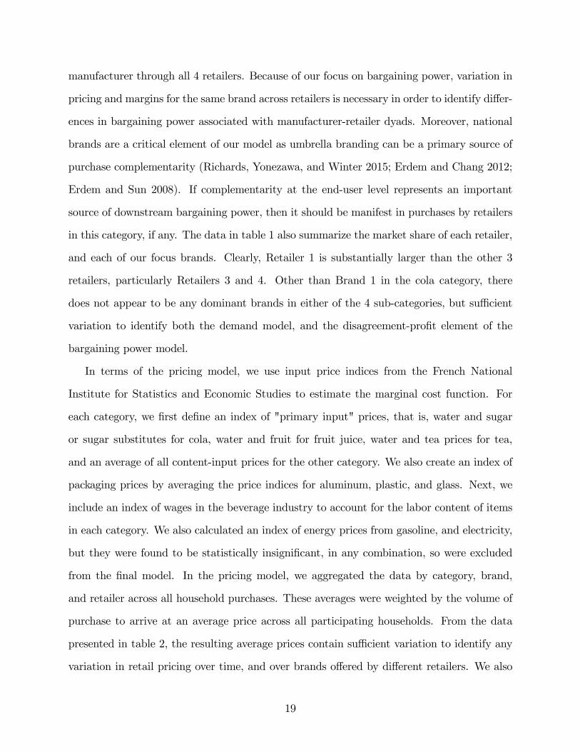
manufacturer through all 4 retailers. Because of our focus on bargaining power, variation in
pricing and margins for the same brand across retailers is necessary in order to identify di¤er-
ences in bargaining power associated with manufacturer-retailer dyads. Moreover, national
brands are a critical element of our model as umbrella branding can be a primary source of
purchase complementarity (Richards, Yonezawa, and Winter 2015; Erdem and Chang 2012;
Erdem and Sun 2008). If complementarity at the end-user level represents an important
source of downstream bargaining power, then it should be manifest in purchases by retailers
in this category, if any. The data in table 1 also summarize the market share of each retailer,
and each of our focus brands. Clearly, Retailer 1 is substantially larger than the other 3
retailers, particularly Retailers 3 and 4. Other than Brand 1 in the cola category, there
does not appear to be any dominant brands in either of the 4 sub-categories, but su¢ cient
variation to identify both the demand model, and the disagreement-pro�t element of the
bargaining power model.
In terms of the pricing model, we use input price indices from the French National
Institute for Statistics and Economic Studies to estimate the marginal cost function. For
each category, we �rst de�ne an index of "primary input" prices, that is, water and sugar
or sugar substitutes for cola, water and fruit for fruit juice, water and tea prices for tea,
and an average of all content-input prices for the other category. We also create an index of
packaging prices by averaging the price indices for aluminum, plastic, and glass. Next, we
include an index of wages in the beverage industry to account for the labor content of items
in each category. We also calculated an index of energy prices from gasoline, and electricity,
but they were found to be statistically insigni�cant, in any combination, so were excluded
from the �nal model. In the pricing model, we aggregated the data by category, brand,
and retailer across all household purchases. These averages were weighted by the volume of
purchase to arrive at an average price across all participating households. From the data
presented in table 2, the resulting average prices contain su¢ cient variation to identify any
variation in retail pricing over time, and over brands o¤ered by di¤erent retailers. We also
19
impute a promotion variable at the household level by measuring the di¤erence in price
for the same brand at the same retailer from one week to the next. Any price di¤erence
that is larger than -10%, and remains for 1 week, is de�ned as a temporary price reduction,
or a promotion. Table 2 presents summary statistics for all input prices, item prices, and
promotional activity.
[table 2 in here]
In the demand model, prices are likely to be endogenous (Villas-Boas and Winer 1999).
That is, at the household level, the error term for each demand equation contains some
information that the retailer observes in setting equilibrium prices: advertising, in-store dis-
plays, preferred shelf-space, or a number of other factors that we do not observe in our data.
Therefore, we estimate the demand model using the control function method (Petrin and
Train 2010). Essentially, the control function approach consists of using the residuals from
a �rst-stage instrumental variables regression as additional variables on the right-side of the
demand model. Because the residuals from the instrumental variables regression contain
information on the part of the endogenous price variable that is not explained by the in-
struments, they have the e¤ect of removing the correlated part from the demand equation.
Because input prices are expected to be correlated with retail prices, and yet independent
of demand, our �rst-stage control function regression uses the set of input price variables
as instruments. We also include brand and retailer �xed-e¤ects in order to account for any
endogenous e¤ects that are unique to each item. Although these variables should represent
e¤ective instruments, whether they are weak in the sense of Staiger and Stock (1997) is
evaluated on the basis of the F-test that results from the �rst-stage instrumental variables
regression.9 In this case, the F-statistic is 65:4, which is much larger than the threshold of
10:0 suggested by Staiger and Stock (1997). Therefore, we conclude that our instruments
are not weak.
We can also draw some stylized facts from our demand data. Our interest in studying
9Detailed results from the �rst-stage instrumental variables regression are available from the authors.
20

the structural e¤ects of complementarity on bargaining power follows from a simple obser-
vation: In our soft-drink data, when items from di¤erent categories are purchased together,
consumers appear to be willing to pay a signi�cant price-premium for either product, relative
to their respective category averages (�gure 1). That is, if a consumer purchases only a fruit
juice, they would be willing to pay more for the same fruit juice if they also purchased at
least one item from another category.10 While there are many factors that may explain this
di¤erence, it is suggestive of a pattern that consumers are willing to pay more for items when
combined in a shopping basket, than when purchased alone.11 Whether this represents a
greater demand for complementary items remains to be determined by estimating the MVL
model described above, and calculating equilibrium prices for complementary items.
[�gure 1 in here]
5 Results and Discussion
In this section, we �rst present the results from estimating several versions of the MVL
shopping-basket model, and then the estimates from the Nash bargaining-equilibrium model.
All bargaining-power estimates are conditioned on the preferred speci�cation for demand,
in order to ensure that our estimates are consistent across all of the models used. Because
we are able to use these estimates to derive a vector of bargaining-power estimates across
each category-retailer-brand observation, we then present the results from a supplementary
regression of bargaining power on the extent of complementarity associated with each item.
In this way, we are able to test our primary hypothesis regarding the relationship between
complementarity and bargaining power.
10The di¤erences are statistically signi�cant at the 5% level for the juice, iced tea, and other categories,and at 15% for the cola category.11We considered the possibility that this observation was due to the fact that single-category purchases
are likely to involve greater quantities, and hence lower unit prices. However, consumers in our samplepurchased greater quantities only during multi-category shopping trips for 2 of the 4 categories.
21
5.1 Demand Model Results
Our demand-model estimates are shown in tables 3 and 4 below. Table 3 presents the
structural estimates for each baseline-utility model, while table 4 presents the full set of
interaction parameters, estimated from the same model. In each case, we compare the
estimates from a �xed coe¢ cient version of the MVL model to one that takes unobserved
heterogeneity explicitly into account by including random coe¢ cients for both the marginal
utility of income, and the category-interaction parameters. A likelihood ratio (LR) test
comparing the �xed and random-coe¢ cient versions of the model yields a test-statistic value
of 186:2, whereas the critical Chi-square value at 5% and 7 degrees of freedom is 14:07, so
we interpret the results from the preferred, random-coe¢ cient version of the model.
[table 3 in here]
Comparing the estimates between the two models also shows the extent of bias from not
accounting for unobserved heterogeneity, as the marginal utility of income, for example, is
nearly 1/3 as large in the random-coe¢ cient relative to the �xed-coe¢ cient model.12 Among
the other parameters of interest in the demand model, note that inventory has a strong,
negative e¤ect on the probability that a shopping basket contains each category, except in
the case of fruit juice. Because fruit juice is the least storable of any category included here,
this result is intuitive. Further, promotion generally has a strong, positive e¤ect on demand
in each category but tea. Although an interaction term between price and promotion could
not be identi�ed in our data, it is likely the case that promoting tea caused the demand curve
to rotate, or become more elastic, su¢ cient to cause the net e¤ect on category-demand to
become negative. In each case, the control function parameter was statistically signi�cant,
which implies that endogeneity is an important feature of our data. Of more interest with
this model, however, is the sign and signi�cance of utility-interactions among categories.
Based on the estimates in table 4, we conclude that there are signi�cant interaction ef-
12Note that we restrict the marginal utility of income to be equal across all categories as, logically, thisparameter is an attribute of household preferences and should not vary across categories.
22

fects associated with purchasing items from di¤erent categories together in the same shopping
basket. In fact, because each mean-estimate is positive, these results suggest that comple-
mentarity is rather the rule than the exception. Because the scale parameter associated with
4 of the 6 interaction-pairs are negative, however, many of the point-estimates for speci�c
items will indeed be negative in total. This is particularly true for the Cola, Fruit Juice in-
teraction parameter, and the Fruit Juice, Other interaction parameter, which show relatively
large scale estimates. In general, the statistical signi�cance of these interaction parameters
suggests that models that do not allow for utility-interaction among category purchases are
fundamentally mis-speci�ed as complementarity is likely to be important. Our interest in
this paper, however, does not lie in identifying complementarity per se, but rather its impact
on equilibrium pricing, and bargaining power. We examine these e¤ects in the next section.
[table 4 in here]
5.2 Bargaining Power Results
Our empirical bargaining power model is structural in nature in the sense that describes how
the total margin (retail price less production and distribution cost) is allocated between the
manufacturer and retailer, and the bargaining power parameter is identi�ed by variation in
the rate at which changes in cost are passed-through to the retail level. Estimates from the
base bargaining power model, and a �xed-coe¢ cient alternative, are shown in table 5. Similar
to our approach in evaluating the importance of unobserved heterogeneity for the demand
model, we conduct a LR speci�cation test in order to determined the preferred form of the
pricing model. Using the results in table 5, the Chi-squared LR statistic is 1; 180:2, while the
critical value is 3:84 with on degree of freedom. Consequently, we reject the �xed coe¢ cient
version and interpret the bargaining power estimates allowing for random variation of the
bargaining power parameter. From a practical perspective, allowing � to vary over time by
retailer also allows us to identify factors that may or may not be associated with variation
in market power over time.
23
[table 5 in here]
The bargaining-power estimates are found after controlling for variation in input prices,
and retailer-�xed e¤ects. Interpreted at the mean of the � point-estimates, we �nd that
retailers earn approximately 2=3 of the total margin across all of our sample beverage cate-
gories.13 This �nding is somewhat surprising, given the importance of large, multi-national
beverage manufacturers such as Coca Cola and Pepsico, but re�ects the fundamental eco-
nomics of selling through oligopoly retail channels. Although net margins in the retailing
industry may be traditionally low, these �ndings suggest that retailers still earn a relatively
large share of the price-cost margin, but much of these rents are absorbed by the �xed costs
of retailing.
5.3 Bargaining Power and Complementarity
The point estimate in table 5, however, does not tell us anything about the relationship be-
tween bargaining power and complementarity. Ailawadi, et al. (2010), however, argue that
explaining variation in bargaining power is an important insight that needs to come out of
the vertical relationships literature. Therefore, we present the results from a supplementary
regression of bargaining power on a measure of complementarity, and retailer �xed e¤ects,
in table 6. Our primary hypothesis concerns the empirical relationship between bargaining
power and complementarity. Complementarity means that retailers, who internalize pric-
ing externalities from selling products that are related in demand, earn lower margins on
complementary products (Rhodes 2015; Zhou 2014) relative to items that are substitutes
in demand. Therefore, retailers�disagreement pro�t is lower for complementary products.
Manufacturers negotiate with retailers�incentives �rmly in mind, so complementarity should
imply more retailer bargaining power, and lower manufacturer power, relative to the usual
substitute-products case.
We investigate this question in table 6, in which we estimate a model that shows how � to
13Note, however, that this does not mean that retailers earn fully 2=3 of the pro�t as manufacturers earnsome of the disagreement pro�t according to equation (15), depending on the re-allocation of demand.
24
varies over retailers, and with the degree of complementarity. In this table, Model 1 considers
the possibility that retailers� bargaining power erodes over time, while Model 2 removes
the time-decay e¤ect. Model 3 includes a binary indicator (Cat �Mfg) that captures the
e¤ect of manufacturers that sell items in multiple categories. From the estimates reported
in this table, we �nd support for our hypothesis. Namely, because the COMP variable
is continuously valued, and negative for a product that complements others, these results
suggest that complementary products are associated with a share of the total margin that is
approximately 28% greater from the retailers�perspective, ceteris paribus. Said di¤erently, if
an item is complementary with other items, then that item is associated with a share of the
total margin that is almost one-third higher for the retailer compared to a di¤erent item that
tends to substitute for others. Although we allowed for the possibility that retailer bargaining
power also erodes over time, we failed to reject the null hypothesis of no time-dependency
over time. Although it is likely that bargaining power does change over a longer time-
series, a one-year time period is not su¢ cient to capture changes in retailer-manufacturer
relationships in our data.
[table 6 in here]
The estimates in table 6 also show that Retailers 2 and 3 appear to be slightly more
successful in bargaining with the set of manufacturers in our data compared to Retailer
1. While we cannot disclose the identity of the retailers, Retailers 2 and 3 are far larger,
measured by sales, relative to Retailer 1, so a high degree of bargaining power is perhaps to
be expected. This �nding also suggests that there is a substantial component of the variation
in bargaining power that is due to di¤erences in size, managerial e¤ectiveness, product-mix,
geographical distribution or other factors that a¤ect performance in the vertical channel.
Manufacturers may also o¤er items across-categories, whether complementary or not.
There are two possible e¤ects on their bargaining power: First, if a manufacturer o¤ers a
number of "must have" national brands in key categories, then it may be the case that
manufacturer barganing power rises if it controls brands in a number of categories. Second,
25

a manufacturer may o¤er a "full line forcing" or bundling arrangement in order to ensure
that the retailer provides its brands as wide of coverage as possible. Ho, Ho, and Mortimer
(2012) �nd that such an arrangement in the video rental industry is responsible for lower
wholesale prices, and, often, lower supplier pro�ts. When we estimate a version of the
bargaining power model in which we control for both complementarity and a binary indicator
for multi-category presence (Model 3), we �nd empirical support for the �ndings of Ho, Ho,
and Mortimer (2012).14 That is, a multi-category presence is associated with higher retailer
bargaining power, so it appears as though manufacturers in the soft drink industry are willing
to give up value in order to secure broad coverage for all their brands.
The analysis in tables 6, however, concerns only the exogenous part of bargaining power,
or the � parameter that divides the share of the total margin into the part earned by the
retailer, and the part earned by the manufacturer. How the level of each margin varies
with complementarity, however, is also of interest. We o¤er some evidence in that regard in
table 7. In this table, we calculate the implied total, retail, and manufacturer margins, as
well as the prices received by the retailer. The �ndings in this table show that the positive
relationship between complementarity and retailer bargaining power appears to be driven
largely by two categories �colas and fruit juice �while bargaining power in the other two
categories is more equally shared. From the summary statistics in table 1, it is clear that
the majority of shopping baskets that contain soft drinks consist of some combination of
colas and fruit juices. Therefore, if complementarity is indeed an important in�uence on
the balance of negotiating power between retailers and manufacturers, it is likely to involve
these two categories. Further, total margins in the cola and fruit juice categories appear
to be substantially smaller for items that have a complementary relationship with others
relative to those that have a substitute relationship, even when, in the case of fruit juice,
the average retail price is higher. This �nding suggests that retailers and manufacturers are
willing to take smaller margins on items that drive tra¢ c to other, more pro�table categories.
14The speci�c estimates are available from the authors upon request.
26
Nonetheless, this table shows that bargaining power, and margins, di¤er considerably among
categories.
[table 7 in here]
Our �ndings are critical to outcomes for vertical relationships in the food industry, but are
also relevant to a broad class of retailer-manufacturer relationships. Because food is typically
purchased from multi-product retailers, in combinations that include many di¤erent pairs
of complements and substitutes, the supermarket case represents an ideal context in which
to investigate our research question. But, many types of manufacturers sell complemen-
tary items into oligopolistic retail channels, whether the context is computer accessories and
hardware (Dell, Lenovo), sporting goods and accessories or apparel (Adidas, Specialized),
or farm equipment and data services (John Deere, New Holland). In each case, retailers
have expanded over time to take advantage of the incentives inherent in multi-product re-
tailing �generally de�ned as economies of scope and scale �but there has been no research
to this point that identi�es bargaining power as an additional explanation for the expan-
sion of multi-category retailers. In fact, as retailers begin to sell through multiple channels,
including online, bricks-and-mortar, and print-catalogue, the complementarity inherent in
cross-channel selling may further manifest in even higher retailer margins through the mech-
anism we identify.
6 Conclusion and Implications
In this paper, we investigate the role of complementarity in in�uencing the relative bargaining
power between retailers and manufacturers in a vertical channel. Based on theoretical models
of bargaining in a vertical channel, with multi-product retailers and manufacturers (Horn
and Wolinsky 1988) we expect that the nature of demand relationships in the downstream
market are critically important to how bargaining power manifests in the share of the price-
cost margin earned by each party. Namely, we expect downstream complementarity to be
associated with higher levels of retailer bargaining power as manufacturers�disagreement
27
pro�t is lower if products are purchased together by consumers in the retail market. Lower
disagreement pro�t means that manufacturers have an incentive to reach agreements to
sell complementary products through their retail partners, and retailers negotiate with this
understanding in mind.
We test our hypothesis using a new model of shopping-basket demand that accounts for
both the discrete nature of category-level purchases, and the complementarity associated
with combining items from several categories on each trip to the store. The MVL model
is able to capture the observation that some pairs of items from di¤erent categories tend
to be purchased together, even when they are not complements in the traditional sense
of bread-and-better, or ketchup-and-hamburger. We apply the MVL model to a sample
household-level data from four soft-drink categories purchased by French households in the
2013 calendar year, focusing on purchases made by households at the top four retail chains,
buying the top four brands sold across all retailers.
We �nd that selling complementary product pairs is associated with roughly 9% greater
retailer margin-share than would otherwise be the case. That is, retailers are able to enhance
their bargaining power relative to manufacturers by selling complementary products across
categories. When entering negotiations, retailers understand that manufacturers have to
o¤er a broad array of items across di¤erent categories in order to extend their brand appeal.
Knowing the pressures faced by manufacturers, retailers negotiate accordingly, and are able
to extract greater rents in the vertical channel by leveraging the fundamental economics of
multi-product selling.
Our �ndings are likely relevant to other markets in which retail complementarity is im-
portant. As brands expand across related categories, and even related channels, retailers will
be able to take advantage of the fact that manufacturers need to be omni-present in order
to stay in the minds of consumers. Whether in the technology, sports, industrial equipment,
or other markets, retailers share a common attribute of being the primary means by which
manufacturers are able to reach consumers �consumers who prefer to purchase goods from
28
one outlet.
Our research is not without limitations. First, we focus our empirical analysis on a single
super-category of items, namely soft drinks. Future research that extends our approach to
data from other food categories, or even other categories of non-food products, would be
valuable. Second, our analysis is restricted to the particular context of French retailing. For
our results to generalize beyond the French context, the nature of bargaining relationships
between manufacturers and retailers would have to be at least similar. Third, our �ndings
are also limited to the European case where anti-trust restrictions to not shape retailer-
manufacturer bargaining, as the Robinson-Patman Act does, at least nominally, in the U.S.
Given the weakness of the Robinson-Patman law, however, it would be of real interest to
use the approach described here to examine the e¤ectiveness of the law itself (Luchs et al.
2010).
29
References
[1] Ailawadi, K.L., Bradlow, E.T., Draganska, M., Nijs, V., Rooderkerk, R.P., Sudhir, K.,
Wilbur, K.C. and Zhang, J., 2010. Empirical models of manufacturer-retailer interac-
tion: A review and agenda for future research. Marketing Letters, 21(3), 273-285.
[2] Besag, J. (1974). Spatial interaction and the statistical analysis of lattice systems. Jour-
nal of the Royal Statistical Society. Series B (Methodological), 36, 192-236.
[3] Binmore, K., A. Rubinstein, and A. Wolinsky. (1986). The Nash bargaining solution in
economic modelling. RAND Journal of Economics, 17, 176-188.
[4] Bucklin, R. E., and J. M. Lattin. (1992). A model of product category competition
among grocery retailers. Journal of Retailing, 68, 271-287.
[5] Bulow, J, J. Geanakoplos, and P. Klemperer. (1985). Multimarket oligopoly: strategic
substitutes and complements. Journal of Political Economy, 93, 488-511.
[6] Bonnet, C., and P. Dubois. (2010). Inference on vertical contracts between manufac-
turers and retailers allowing for nonlinear pricing and resale price maintenance. RAND
Journal of Economics, 41(1), 139-164.
[7] Bonnet, C. and Z. Bouamra-Mechemache (2016). Organic label, bargaining power, and
pro�t-sharing in the French �uid milk market. American Journal of Agricultural Eco-
nomics, 98(1), 113-133.
[8] Cressie, N. A.C. (1993). Statistics for spatial data. New York: John Wiley and Sons.
[9] Draganska, M., Klapper, D., and S. B. Villas-Boas. (2010). A larger slice or a larger pie?
An empirical investigation of bargaining power in the distribution channel. Marketing
Science, 29(1), 57-74.
[10] Dubé, J. P. (2004). Multiple discreteness and product di¤erentiation: Demand for car-
bonated soft drinks. Marketing Science, 23(1), 66-81.
30
[11] Dubé, J. P. (2005). Product di¤erentiation and mergers in the carbonated soft drink
industry. Journal of Economics & Management Strategy, 14(4), 879-904.
[12] Dukes, A., E. Gal-Or, K. Srinivasan. (2006). Channel bargaining with retailer assymetry.
Journal of Marketing Research, 18, 84�97.
[13] Erdem, T., and B. Sun. (2002). An empirical investigation of the spillover e¤ects of
advertising and sales promotions in umbrella branding. Journal of Marketing Research,
39, 1�16.
[14] Erdem, T., S. R. Chang. (2012). A cross-category and cross-country analysis of umbrella
branding for national and store brands. Journal of the Academy of Marketing Science,
40, 86-101.
[15] Feng, Q., and L. X. Lu. (2013a). Supply chain contracting under competition: Bilateral
bargaining vs. Stackelberg. Production and Operations Management, 22(3), 661-675.
[16] Feng, Q., and L. X. Lu. (2013b). The role of contract negotiation and industry structure
in production outsourcing. Production and Operations Management, 22(5), 1299-1319.
[17] Haucap, J., Heimesho¤, U., Klein, G. J., Rickert, D., and C. Wey. (2013). Bargaining
power in manufacturer-retailer relationships (No. 107). DICE Discussion Paper, Dus-
seldorf, Germany.
[18] Ho, K., Ho, J., J. H. Mortimer. (2012). The use of full-line forcing contracts in the video
rental industry. American Economic Review, 102(2), 686-719.
[19] Horn, H., and A. Wolinsky. (1988). Bilateral monopolies and incentives for merger.
RAND Journal of Economics, 408-419.
[20] Iyer, G., M. Villas-Boas. (2003). A bargaining theory of distribution channels. Journal
of Marketing Research, 40, 80�100.
31
[21] Kamakura, W. A., and K. Kwak. (2012). Menu-choice modeling. Working paper, De-
partment of Marketing, Rice University, Houston, TX.
[22] Kwak, K., S. D. Duvvuri, and G. J. Russell. (2015). An analysis of assortment choice
in grocery retailing. Journal of Retailing, 91, 19-33.
[23] Luchs, R., Geylani, T., Dukes, A., & Srinivasan, K. (2010). The end of the Robinson-
Patman act? Evidence from legal case data. Management Science, 56(12), 2123-2133.
[24] Manchanda, P., A. Ansari, S. Gupta. (1999). The shopping basket: A model for multi-
category purchase incidence decisions. Marketing Science, 18, 95�114.
[25] Mehta, N. (2007). Investigating consumer�s purchase incidence and brand choice deci-
sions across multiple categories: a theoretical and empirical analysis.Marketing Science,
26, (2), 196�217.
[26] Meza, S., and K. Sudhir. (2010). Do private labels increase retailer bargaining power?
Quantitative Marketing and Economics, 8(3), 333-363.
[27] Misra, S., S. Mohanty. (2006). Estimating bargaining games in distribution channels.
Working paper, University of Rochester, Rochester, NY.
[28] Moon, S. and G. J. Russell. (2008). Predicting product purchase from inferred customer
similarity: an autologistic model approach. Management Science, 54, 71�82.
[29] Petrin, A. and K. Train. (2010): A control function approach to endogeneity in consumer
choice models. Journal of Marketing Research 47, 3-13.
[30] Rhodes, A. (2015). Multiproduct retailing. The Review of Economic Studies, 82, 360-
390.
[31] Richards, T. J., M. I. Gómez, and G. Pofahl. (2012). A multiple-discrete/continuous
model of price promotion. Journal of Retailing, 88(2), 206-225.
32

[32] Richards, T., K. Yonezawa, and S. Winter, S. (2014). Cross-category e¤ects and private
labels. European Review of Agricultural Economics, 42, 187-216.
[33] Richards, T. J. and S. F. Hamilton. (2016). Retail market power in a shopping basket
model of supermarket competition. Working paper, W. P. Carey School of Business,
Arizona State University, Tempe, AZ.
[34] Russell, G. J. and A. Petersen. (2000). Analysis of cross category dependence in market
basket selection. Journal of Retailing, 76, 367�92.
[35] Singh, V. P., K. T. Hansen, and S. Gupta. (2005). Modeling preferences for common
attributes in multicategory brand choice. Journal of Marketing Research, 42(2), 195-209.
[36] Smith, H., O. Thomassen. (2012). Multi-category demand and supermarket pricing.
International Journal of Industrial Organization, 30, 309-314.
[37] Song, I. and P. K. Chintagunta. (2006). Measuring cross-category price e¤ects with
aggregate store data. Management Science, 52, 1594�609.
[38] Staiger, D., and Stock, J. H. (1997). Instrumental variables regression with weak instru-
ments. Econometrica, 65, 557-586.
[39] Villas-Boas, S. B. (2007). Vertical relationships between manufacturers and retailers:
Inference with limited data. Review of Economic Studies, 74(2), 625�652.
[40] Villas-Boas, M., R. Winer. (1999). Endogeneity in brand choice models. Management
Science, 45(10), 1324�1338.
[41] Villas-Boas, M., Y. Zhao. (2005). Retailers, manufacturers, and individual consumers:
Modeling the supply side in the ketchup marketplace. Journal of Marketing Research,
42(1), 83�95.
[42] Villas-Boas, S. (2007). Vertical contracts between manufacturers and retailers: inference
with limited data. Review of Economic Studies, 74, 625-652.
33
[43] Zhou, J. (2014). Multiproduct search and the joint search e¤ect. American Economic
Review, 104, 2918�2939.
34

Table 1. Summary of Sample SharesRetailers / Brands Baskets
Variable Mean Std. Dev. Variable Mean Std. Dev.
Retailer 1 0.353 0.478 Cola Only 0.088 0.284Retailer 2 0.278 0.448 Fruit Juice Only 0.310 0.462Retailer 3 0.190 0.393 Iced Tea Only 0.014 0.119Retailer 4 0.179 0.384 Other Soft Drink Only 0.082 0.275Brand 1, Category 1 0.300 0.458 Cola and Juice 0.098 0.297Brand 2, Category 1 0.031 0.172 Cola and Tea 0.005 0.068Brand 3, Category 1 0.001 0.030 Cola and Other 0.055 0.229Brand 4, Category 1 0.022 0.147 Juice and Tea 0.017 0.130Brand 1, Category 2 0.171 0.377 Juice and Other 0.134 0.340Brand 2, Category 2 0.071 0.257 Tea and Other 0.008 0.090Brand 3, Category 2 0.044 0.204 Cola, Juice, and Tea 0.017 0.130Brand 4, Category 2 0.004 0.063 Cola, Juice, and Other 0.105 0.307Brand 1, Category 3 0.074 0.261 Cola, Tea, and Other 0.005 0.073Brand 2, Category 3 0.013 0.115 Juice, Tea, and Other 0.028 0.164Brand 3, Category 3 0.003 0.055 Cola, Juice, Tea, and Other 0.032 0.177Brand 4, Category 3 0.065 0.476Brand 1, Category 4 0.066 0.248Brand 2, Category 4 0.059 0.237Brand 3, Category 4 0.046 0.209Brand 4, Category 4 0.016 0.125Note: Brand and retailer identities cannot be disclosed.
35

Table 2. Summary of Soft Drink Pricing DataVariable Units Mean Std. Dev. Min. Max. N
Aluminum Price Index 93.800 4.989 86.700 102.400 3328Plastic Price Index 106.300 0.332 105.700 106.900 3328Glass Price Index 104.967 0.661 103.500 105.700 3328Sugar Price Index 147.106 7.636 134.100 158.500 3328Gasoline Price Index 113.156 2.265 110.300 118.000 3328Electricity Price Index 115.331 4.921 107.300 121.300 3328Sugar Substitute Price Index 104.588 0.700 103.510 106.010 3328Fruit Price Index 2.578 0.115 2.433 2.778 3328Tea and Co¤ee Price Index 114.602 1.001 112.600 116.000 3328Bottled Water Price Index 110.010 0.533 108.500 110.800 3328Beverage Industry Wage Index 110.650 0.415 110.000 111.100 3328Cola Price Euros / liter 0.891 0.245 0.295 1.808 3328Fruit Juice Price Euros / liter 1.855 0.538 0.756 3.333 3328Iced Tea Price Euros / liter 0.918 0.221 0.226 2.500 3328Other Soft Drink Price Euros / liter 1.106 0.405 0.212 9.909 3328Cola Promotion % 0.060 0.238 0.000 1.000 3328Fruit Juice Promotion % 0.052 0.222 0.000 1.000 3328Iced Tea Promotion % 0.064 0.244 0.000 1.000 3328Other Soft Drink Promotion % 0.070 0.255 0.000 1.000 3328Note: Input prices used to form indices in the �nal estimated model. Promotion indicators calcu-
lated using price-reduction threshold of 10%.
36

Table 4. Interaction Parameters from MVLFixed Coe¢ cient Random Coe¢ cientEstimate t-ratio Estimate t-ratio
Cola, Fruit Juice 48.4471* 78.4467 59.2950* 96.0119Scale -13.8800* -49.5913Cola, Tea 97.7647* 251.6550 45.9108* 118.1784Scale -8.4682* -99.9394Cola, Other 76.0721* 177.6280 42.6219* 99.5219Scale -1.0608* -3.9993Fruit Juice, Tea 89.2720* 271.4451 73.5761* 223.7192Scale 21.6681* 5.1517Fruit Juice, Other 63.3418* 165.5473 77.2406* 201.8725Scale -18.9383* -37.2703Tea, Other 40.8367* 95.1759 36.4701* 84.9990Scale 3.2041 1.5656Note: A single asterisk indicates signi�cance at a 5% level.
37

Table3.MVLDemandEstimates
FixedCoe¢cients
RandomCoe¢cients
FixedCoe¢cients
RandomCoe¢cients
Category
Variable
Estimate
t-ratio
Estimate
t-ratio
Estimate
t-ratio
Estimate
t-ratio
Price
-10.3737
-122.4276
-2.9824
-35.1971
Std.Dev.
1.4678
1.7505
Colas
Constant
-6.0480
-21.6088
-3.6304
-12.9709
Tea
Constant
2.2721
5.1544
-4.0582
-9.2063
Promotion
20.5123
77.3327
11.0433
41.6340
Promotion
-2.5425
-6.1794
-7.6689
-18.6389
HHSize
-56.1220
-13.3433
0.8892
0.2114
HHSize
-65.1401
-13.4826
146.6066
30.3445
Income
-0.9482
-1.8660
7.4980
14.7560
Income
1.4321
1.6988
2.3930
2.8387
Education
-5.7064
-2.7882
-73.9114
-36.1135
Education
-96.3142
-39.4185
-47.4332
-19.4130
Inventory
-134.3834
-16.0262
-157.1277
-18.7387
Inventory
-165.2920
-17.5644
-212.1655
-22.5453
Retailer2
-1.6959
-5.4678
-14.9241
-48.1185
Retailer2
-1.7250
-4.5174
-23.8198
-62.3808
Retailer3
-4.8390
-11.5203
2.6727
6.3631
Retailer3
0.4224
1.1767
0.9384
2.6144
Retailer4
-8.4185
-61.4891
2.2564
16.4810
Retailer4
-0.0597
-0.3504
7.5996
44.6397
Brand1
36.4939
130.7971
28.5176
102.2093
Brand1
39.9710
53.1157
53.1672
70.6515
Brand2
2.3531
8.0344
5.1927
17.7297
Brand3
4.2490
8.6083
10.1732
20.6103
Brand3
-27.6063
-9.3762
-34.8226
-11.8271
Brand4
-6.6287
-24.8196
-13.7564
-51.5075
Brand4
58.0533
177.6811
-2.8304
-8.6630
CF
-10.6674
-38.1133
-15.3591
-49.5210
CF
-17.0717
-64.3616
-26.4124
-192.9166
FruitJuice
Constant
-1.9568
-7.9419
-2.0928
-8.4939
Other
Constant
-4.8275
-17.8587
-3.3627
-12.4400
Promotion
5.0975
44.2928
15.3943
133.7640
Promotion
15.6611
92.7254
11.9560
70.7881
HHSize
-164.2370
-45.4800
-102.8920
-28.4925
HHSize
-104.8114
-24.6190
-71.5824
-16.8139
Income
10.4865
31.8333
13.0656
39.6625
Income
3.7661
11.0882
7.8993
23.2571
Education
-19.4736
-11.0123
-45.6109
-25.7928
Education
-8.1430
-4.0154
-43.7277
-21.5625
Inventory
54.4302
4.5909
122.5980
10.3404
Inventory
33.1227
3.2762
-12.7122
-1.2574
Retailer2
-1.4999
-5.3536
-14.8281
-52.9280
Retailer2
-2.4039
-8.2860
-15.8365
-54.5862
Retailer3
-5.7978
-17.5062
1.6649
5.0270
Retailer3
-5.7158
-16.9274
1.8109
5.3630
Retailer4
-7.3244
-64.0657
2.4833
21.7211
Retailer4
-7.3527
-56.1555
2.4551
18.7506
Brand2
11.2502
0.2847
34.7106
0.8783
Brand1
7.1033
15.8607
7.5656
16.8928
Brand3
3.0818
21.9648
20.7182
147.6651
Brand2
184.8058
126.2629
19.4588
13.2946
Brand4
45.1965
134.4622
2.5195
7.4958
Brand3
10.4618
60.6124
6.0893
35.2797
CF
8.8679
104.6567
0.8377
1.9943
Brand4
6.5542
16.5531
5.6731
14.3279
CF
7.0862
1.6848
-0.0690
-0.2474
LLF/AIC
-2324.5900
0.0348
-2231.46
0.0334
Note:CFisthecontrolfunctionparameter.Asingleasteriskindicatessigni�canceat5%.
38
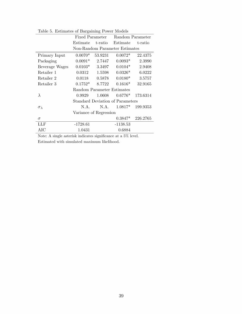
Table 5. Estimates of Bargaining Power ModelsFixed Parameter Random ParameterEstimate t-ratio Estimate t-ratioNon-Random Parameter Estimates
Primary Input 0.0070* 53.9231 0.0072* 22.4375Packaging 0.0091* 2.7447 0.0093* 2.3990Beverage Wages 0.0103* 3.3497 0.0104* 2.9408Retailer 1 0.0312 1.5598 0.0326* 6.0222Retailer 2 0.0118 0.5878 0.0180* 3.5757Retailer 3 0.1752* 8.7722 0.1616* 32.9165
Random Parameter Estimates� 0.9929 1.0608 0.6776* 173.6314
Standard Deviation of Parameters�� N.A. N.A. 1.0817* 199.9353
Variance of Regression� 0.3847* 226.2765LLF -1728.61 -1138.53AIC 1.0431 0.6884Note: A single asterisk indicates signi�cance at a 5% level.
Estimated with simulated maximum likelihood.
39

40

Table6.BargainingPowerandComplementarity
Model1
Model2
Model3
Retailer1
0.3540*
8.4495
0.3540*
8.4556
0.3169*
7.0454
Retailer2
0.3848*
9.5946
0.3848*
9.5946
0.3601*
8.6447
Retailer3
0.3924*
9.6484
0.3924*
9.6484
0.3615*
8.5249
Cat*Mfg
0.0988*
2.2599
Complementarity
-0.2792
-1.8632
-0.2781*
-3.7868
-0.2792*
-3.7932
Comp*Time
0.0042
0.8714
RandomParameterScale
Complementarity
0.0334
1.4477
0.0334
1.4477
0.0331
1.4420
ParameterVariance
1.1630*
73.0509
1.1630
73.0968
1.1620*
72.9466
LLF
-5224.7921
-5224.7910
-5222.0722
AIC/N
3.2409
3.2409
3.2392
Note:Asingleasteriskindicatessigni�canceata5%
level.
41
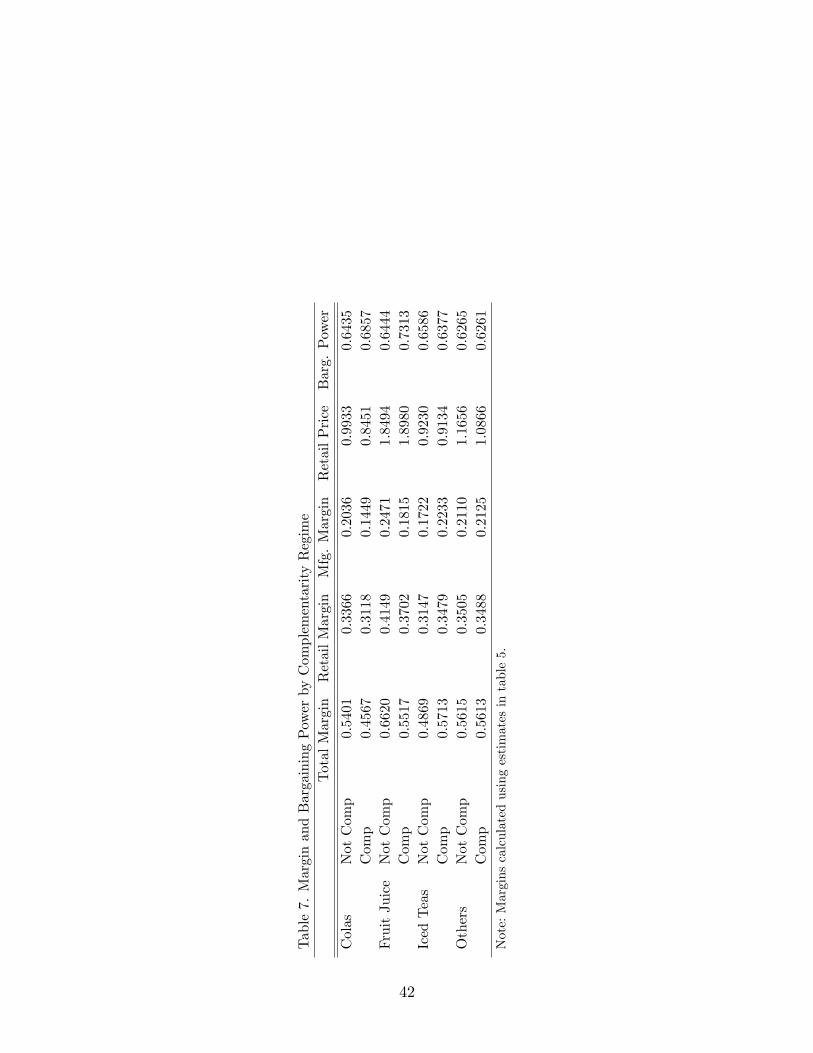
Table7.MarginandBargainingPowerbyComplementarityRegime
TotalMargin
RetailMargin
Mfg.Margin
RetailPrice
Barg.Power
Colas
NotComp
0.5401
0.3366
0.2036
0.9933
0.6435
Comp
0.4567
0.3118
0.1449
0.8451
0.6857
FruitJuice
NotComp
0.6620
0.4149
0.2471
1.8494
0.6444
Comp
0.5517
0.3702
0.1815
1.8980
0.7313
IcedTeas
NotComp
0.4869
0.3147
0.1722
0.9230
0.6586
Comp
0.5713
0.3479
0.2233
0.9134
0.6377
Others
NotComp
0.5615
0.3505
0.2110
1.1656
0.6265
Comp
0.5613
0.3488
0.2125
1.0866
0.6261
Note:Marginscalculatedusingestimatesintable5.
42