2012 Simulations of the DARPA Suboff submarine … · University of Iowa Iowa Research Online...
60
University of Iowa Iowa Research Online eses and Dissertations 2012 Simulations of the DARPA Suboff submarine including self-propulsion with the E1619 propeller Nathan Chase University of Iowa Follow this and additional works at: hp://ir.uiowa.edu/etd Part of the Mechanical Engineering Commons is dissertation is available at Iowa Research Online: hp://ir.uiowa.edu/etd/2837 Recommended Citation Chase, Nathan. "Simulations of the DARPA Suboff submarine including self-propulsion with the E1619 propeller." thesis, University of Iowa, 2012. hp://ir.uiowa.edu/etd/2837.
Transcript of 2012 Simulations of the DARPA Suboff submarine … · University of Iowa Iowa Research Online...

University of IowaIowa Research Online
Theses and Dissertations
2012
Simulations of the DARPA Suboff submarineincluding self-propulsion with the E1619 propellerNathan ChaseUniversity of Iowa
Follow this and additional works at: http://ir.uiowa.edu/etdPart of the Mechanical Engineering Commons
This dissertation is available at Iowa Research Online: http://ir.uiowa.edu/etd/2837
Recommended CitationChase, Nathan. "Simulations of the DARPA Suboff submarine including self-propulsion with the E1619 propeller." thesis, Universityof Iowa, 2012.http://ir.uiowa.edu/etd/2837.

Report Documentation Page Form ApprovedOMB No. 0704-0188
Public reporting burden for the collection of information is estimated to average 1 hour per response, including the time for reviewing instructions, searching existing data sources, gathering andmaintaining the data needed, and completing and reviewing the collection of information. Send comments regarding this burden estimate or any other aspect of this collection of information,including suggestions for reducing this burden, to Washington Headquarters Services, Directorate for Information Operations and Reports, 1215 Jefferson Davis Highway, Suite 1204, ArlingtonVA 22202-4302. Respondents should be aware that notwithstanding any other provision of law, no person shall be subject to a penalty for failing to comply with a collection of information if itdoes not display a currently valid OMB control number.
1. REPORT DATE 2012 2. REPORT TYPE
3. DATES COVERED 00-00-2012 to 00-00-2012
4. TITLE AND SUBTITLE Simulations of the DARPA Suboff submarine including self-propulsionwith the E1619 propeller
5a. CONTRACT NUMBER
5b. GRANT NUMBER
5c. PROGRAM ELEMENT NUMBER
6. AUTHOR(S) 5d. PROJECT NUMBER
5e. TASK NUMBER
5f. WORK UNIT NUMBER
7. PERFORMING ORGANIZATION NAME(S) AND ADDRESS(ES) University of Iowa,Iowa City ,IA, 52242
8. PERFORMING ORGANIZATIONREPORT NUMBER
9. SPONSORING/MONITORING AGENCY NAME(S) AND ADDRESS(ES) 10. SPONSOR/MONITOR’S ACRONYM(S)
11. SPONSOR/MONITOR’S REPORT NUMBER(S)
12. DISTRIBUTION/AVAILABILITY STATEMENT Approved for public release; distribution unlimited
13. SUPPLEMENTARY NOTES
14. ABSTRACT Simulations of the DARPA Suboff submarine and the submarine propeller E1619 using the overset flowsolver CFDShip-Iowa V4.5 are presented. The hull was tested in a straight ahead simulation and also in astarboard turn. Propeller open water curves were obtained for two grids for a wide range of advancecoefficients covering high to moderately low loads, and results compared with available experimental data.A verification study was performed for one advance coefficient ( ) on four grids and three time step sizes.The effect of the turbulence model on the wake was evaluated at comparing results with RANS, DES,DDES, and with no turbulence model showing that RANS overly dissipates the wake and that in thesolution with no turbulence model the tip vortices quickly become unphysically unstable. Tip vortexpairing is observed and described for revealing multiple vortices merging for higher loads. The wakevelocities are compared against experimental data for showing good agreement. Self-propulsioncomputations of the DARPA Suboff generic submarine hull fitted with sail, rudders, stern planes, and theE1619 propeller were performed in model scale and the resulting propeller performance analyzed.
15. SUBJECT TERMS
16. SECURITY CLASSIFICATION OF: 17. LIMITATION OF ABSTRACT Same as
Report (SAR)
18. NUMBEROF PAGES
60
19a. NAME OFRESPONSIBLE PERSON
a. REPORT unclassified
b. ABSTRACT unclassified
c. THIS PAGE unclassified
Standard Form 298 (Rev. 8-98) Prescribed by ANSI Std Z39-18

SIMULATIONS OF THE DARPA SUBOFF SUBMARINE INCLUDING SELF-
PROPULSION WITH THE E1619 PROPELLER
by
Nathan Chase
A thesis submitted in partial fulfillment of the requirements for the Master of
Science degree in Mechanical Engineering in the Graduate College
of The University of Iowa
May 2012
Thesis Supervisor: Associate Professor Pablo M. Carrica

Graduate College
The University of Iowa
Iowa City, Iowa
CERTIFICATE OF APPROVAL
_______________________
MASTER’S THESIS
______________
This is to certify that the Master’s thesis of
Nathan Chase
has been approved by the Examining Committee
for the thesis requirement for the Master of Science
degree in Mechanical Engineering at the May 2012 graduation.
Thesis Committee: _____________________________________________
Pablo M. Carrica, Thesis Supervisor
_____________________________________________
Ching-Long Lin
_____________________________________________
Frederick Stern

ii
ACKNOWLEDGEMENTS
I would like to thank my advisor, Dr. Pablo Carrica. His guidance and
encouragement throughout my graduate career has been instrumental. I would also like
to thank my other committee members, Dr. Fred Stern and Dr. Ching-Long Lin, for
taking time out of their schedules to assist me in this process.
I would like to also acknowledge the help I have received from other students at
IIHR-Hydroscience and Engineering and the financial support from the Office of Naval
Research under Grant N000141110232, with Dr. Ki-Han Kim as the program manager.
iii
ABSTRACT
Simulations of the DARPA Suboff submarine and the submarine propeller E1619
using the overset flow solver CFDShip-Iowa V4.5 are presented. The hull was tested in a
straight ahead simulation and also in a starboard turn. Propeller open water curves were
obtained for two grids for a wide range of advance coefficients covering high to
moderately low loads, and results compared with available experimental data. A
verification study was performed for one advance coefficient ( ) on four grids
and three time step sizes. The effect of the turbulence model on the wake was evaluated
at comparing results with RANS, DES, DDES, and with no turbulence model
showing that RANS overly dissipates the wake and that in the solution with no turbulence
model the tip vortices quickly become unphysically unstable. Tip vortex pairing is
observed and described for revealing multiple vortices merging for higher
loads. The wake velocities are compared against experimental data for showing
good agreement. Self-propulsion computations of the DARPA Suboff generic submarine
hull fitted with sail, rudders, stern planes, and the E1619 propeller were performed in
model scale and the resulting propeller performance analyzed.

iv
TABLE OF CONTENTS
LIST OF TABLES ..................................................................................................... v
LIST OF FIGURES .................................................................................................. vi CHAPTER
1 INTRODUCTION .................................................................................. 1 1.1. Background ...................................................................................... 1 1.2. Objectives and Approach ................................................................. 4 2 COMPUTATIONAL METHODS .......................................................... 6 2.1. Overview .......................................................................................... 6 2.2. Mathematical Modeling ................................................................... 6 2.2.1. Governing Equations ............................................................... 6 2.2.2. Turbulence Modeling ............................................................... 7 2.2.3. Numerical Methods and Motion Controller ............................ 8 3 DARPA SUBOFF SUBMARINE ........................................................ 10 3.1. Straight-ahead Simulation ............................................................. 10 3.2. Turning Simulation ........................................................................ 17
4 INSEAN E1619 PROPELLER ............................................................. 22 4.1. Geometry and Simulation Conditions ........................................... 22 4.2. Verification and Validation ........................................................... 26 4.3. Open Water Curve ......................................................................... 28 4.4. Wake Analysis ............................................................................... 30 4.4.1. Grid Comparison ................................................................... 30 4.4.2. Wake Grid .............................................................................. 31
5 SELF-PROPULSION ........................................................................... 38 5.1. Simulation Conditions ................................................................... 38 5.2. Self-propelled Analysis ................................................................. 40 5.3. Blade Analysis ............................................................................... 43 6 CONCLUSIONS AND RECOMMENDATIONS FOR FUTURE
WORK .................................................................................................. 46 6.1. Conclusions.................................................................................... 46 6.2. Recommendations for Future Work .............................................. 47
REFERENCES ........................................................................................................ 48

v
LIST OF TABLES
Table 3.1: DARPA Suboff and David Taylor Research Center Anechoic Flow Facility main parameters ....................................................................... 10
Table 3.2: Grid dimensions for AFF-8 submarine ................................................... 11
Table 3.3: DARPA Suboff fully-appended turning case main parameters .............. 17
Table 3.4: Grid dimensions for AFF-8 submarine turning case .............................. 18 Table 4.1: INSEAN E1619 main propeller parameters ........................................... 22
Table 4.2: Dimensions for grids used for verification study ................................... 24
Table 4.3: Details of the wake grid .......................................................................... 25
Table 4.4: Numerical uncertainty from grid and time step convergence
for .......................................................................................... 28 Table 4.5: Different solver methods at ....................................................... 34
Table 5.1: DARPA Suboff self-propelled by INSEAN E1619 main parameters ... 38
Table 5.2: Grid dimensions for self-propelled grid ................................................. 39
Table 5.3: Self-propelled solution at m/s ................................................ 41
vi
LIST OF FIGURES Figure 3.1: AFF-8 and deep water towing tank grid ................................................ 10
Figure 3.2: Resistance of Suboff Model 5470 ......................................................... 12
Figure 3.3: AFF-8 wake at ................................................................. 13
Figure 3.4: AFF-8 circumferentially averaged velocity at ................ 14 Figure 3.5: AFF-8 shear stress at ....................................................... 14
Figure 3.6: AFF-8 wake at ................................................................... 15
Figure 3.7: AFF-8 wake at ..................................................................... 15
Figure 3.8: View of the DARPA Suboff submarine in straight-ahead case ............ 16 Figure 3.9: Rotating arm submarine turning case .................................................... 17
Figure 3.10: View of the DARPA Suboff submarine in rotating arm turn ............. 19
Figure 3.11: Turn velocity at ............................................................. 19
Figure 3.12: Turn velocity vectors and vorticity at ............................. 20
Figure 3.13: Turn velocity vectors and vorticity at ............................. 21
Figure 4.1: Coarse grid system ................................................................................ 22
Figure 4.2: Wake grid system .................................................................................. 25
Figure 4.3: Convergence history of the thrust coefficient for different grids .......... 26 Figure 4.4: Convergence history of the torque coefficient for different grids ......... 27
Figure 4.5: Grid and time step convergence ............................................................ 27
Figure 4.6: E1619 OWC for wake and fine grids .................................................... 29
Figure 4.7: isosurfaces at for grids using DDES ................. 30 Figure 4.8: Vorticity for all grids at using DDES ................................... 31
Figure 4.9: isosurfaces for different turbulence models at .............................................................................................. 32
Figure 4.10: Vorticity for different turbulence models at ........................... 33
Figure 4.11: Q isosurfaces for all J's using DDES with the wake grid .................... 34
Figure 4.12: Vorticity at different J's using DDES with the wake grid ................... 35
vii
Figure 4.13: Propeller velocity for at (data from Liefvendahl et al. 2010) ........................................................................ 36
Figure 5.1: Grid for self-propelled submarine computations................................... 38 Figure 5.2: Convergence history of boat velocity and propeller rotational speed ... 40
Figure 5.3: Cross sections of the wake at two axial positions (left) and at
(right) for self-propelled submarine ...................................................... 42
Figure 5.4: View of the self-propelled DARPA Suboff submarine with vortical structures as isosurfaces of ............................................... 42
Figure 5.5: Thrust coefficient of three contiguous blades for three full rotations of the propeller. Blade 1 is on top at 0 degrees, with blade 2 the next one to port and blade 7 the previous to starboard ......................... 43 Figure 5.6: Instantaneous wake at an axial location upstream of the propeller. Every 11
th vector is shown for clarity .................................. 45

1
CHAPTER 1
INTRODUCTION
1.1 Background
Propeller performance and efficiency are important parameters for all marine
vehicles, but especially so on a submarine. A submarine propeller is optimized for noise
reduction and therefore has more blades and is relatively larger than a ship propeller
(Felli et al. 2008). Computational Fluid Dynamics (CFD) provides a more cost effective
method of testing new propeller designs compared to Experimental Fluid Dynamics
(EFD) as experimental prototypes are expensive and time consuming to create. CFD also
enables more efficient optimization of propeller design due to shorter design cycles.
Designers can quickly test different blade shapes, sizes, and number of blades without the
cost of unnecessary fabrication. However, numerical simulations must be validated
before extensive use on design and test purposes and CFD is costly compared to other
simulation approaches, like potential flow methods.
Propeller forces have been studied and experimentally tested for over 70 years.
Denny (1968) describes the process of obtaining propeller open water performance as it
was done in the past. Current experimental procedures and corresponding uncertainty
analysis are periodically updated by the International Towing Tank Conference (2002).
Though submarine data is mostly unavailable, experimental results for the generic
submarine propeller INSEAN E1619 were reported by Di Felice et al. (2009), who
studied open water performance and the wake of the propeller under various loads. Pitot
tubes, hot-wire, Laser Doppler Velocimetry (LDV) and Particle Image Velocimetry (PIV)
techniques have all been used to measure the wake of propellers. Inoue and Kuroumaru
(1984) first investigated the structure and decay of vorticity of an impeller flow field
utilizing a slanted single hot-wire. As technology advanced, LDV and PIV have become
the preferred methods for wake analysis as they allow more efficient data acquisition and
easy reconstruction of a flow field cross section (Di Felice et al. 2009, Felli et al. 2011).

2
The most common numerical methodologies for studying propeller flows are
classified as potential flow or CFD approaches although other methods such as actuator
disc can be used. Potential flow models are cheaper and easier to use, however they are
reliable only if minor viscous effects are expected. The relative simplicity of potential
flow codes enabled them to be used when computers were still in their infancy, and thus
have been used longer than CFD codes. CFD is more accurate and can capture the wake
and highly transient effects, but it is considerably more expensive.
A potential flow low-order 3-D boundary element method was used by Young
and Kinnas (2003) to evaluate supercavitating and surface-piercing propellers. The
simulation’s predicted results compare well with experimental measurements for steady
inflow. Fuhs (2005) evaluated PUF-2, PUF-14, MPUF-3A, and PROPCAV solvers with
DTMB propellers 4119, 4661, 4990, and 5168 under different conditions. He found that
none of these potential flow solvers performed significantly better than the others under
non-cavitating conditions.
Gatchell et al. (2011) evaluated open water propeller performance using the
potential flow panel code PPB and the Reynolds averaged Navier-Stokes (RANS) solver
FreSCo+. The codes gave similar results at advance coefficient (J) values higher than 1.3
but PPB dramatically under predicted the torque and thrust at lower J’s. Watanabe et al.
(2003) showed that the RANS solver Fluent version 6.1 predicted thrust and torque
coefficients in agreement with the measurements taken from uniform flow. Califano and
Steen (2011) found that a RANS simulation on a generic propeller provides satisfactory
values when compared to experimental results at low J’s but became inaccurate at higher
J’s. They concluded that the inability of the RANS model to resolve tip vortices was the
cause of the discrepancies. Hsiao and Pauley (1999) attempted to reduce the inaccuracies
of a RANS model by incorporating the Baldwin-Barth turbulence method with RANS
computations to compute tip vortex flows around the P5168 propeller. The general flow
characteristics were in agreement with the measured values but the tip vortex was overly

3
diffused. Rhee and Joshi (2005) also simulated the P5168 propeller utilizing a k-w
turbulence model and found that the thrust and torque values are in good agreement with
measured values, but turbulence quantities in the tip vortex region were under-predicted.
To resolve the unsteady flow field behind a DTMB 4118 propeller, Yu-cun and
Huai-xin (2010) employed Detached-Eddy Simulation (DES) modeling. DES resolves
the tip vortices better than RANS because the turbulent viscosity is reduced where the
grid is fine enough to capture large vortices. The DES calculated open water curve
(OWC) and experimental OWC showed great similarity with the trends being virtually
identical. Yu-cun and Huai-xin (2010) were also able to calculate vortex structures in the
flow and accurately predict the pressure distribution at different blade sections. Castro et
al. (2011) simulated the KP 505 propeller using DES to obtain the OWC and determine
the self-propulsion point for the KRISO container ship KCS. In that case, the OWC was
measured at model-scale but was simulated at full-scale. Despite the differences in
propeller size, the OWCs indicated very good agreement between the simulated and
experimental results.
CFD self-propulsion simulations usually utilize a body force model of the
propeller rather than the direct modeling method used by Carrica et al. (2010, 2011).
Direct modeling is less commonly used because the propeller rotates much faster than the
ship advances, necessitating a small time step to provide sufficient resolution of the
propeller flow. While a body force model provides acceptable results for hull analysis, a
discretized propeller is needed to fully investigate the interaction of wake and appendages
with the propeller. Liefvendahl et al. (2010) and Liefvendahl and Tröeng (2011) used a
Large Eddy Simulation (LES) method to simulate the E1619 propeller wake in both free
stream and under moving conditions using the Defense Advanced Research Projects
Agency (DARPA) Suboff submarine hull near self-propulsion, reporting OWC results as
well as transient loads on the propeller and individual blades. A discretized propeller was

4
also used by Carrica et al. (2010) for a self-propelled ship, and this technique is applied
in this paper to the DARPA Suboff submarine propelled by the E1619 propeller.
The flow around the DARPA Suboff has previously been computed without a
propeller by Bull (1996) and by Rhee (2003). Alin et al. (2010) computed the flow
around the Suboff body both with and without an actuator disk propeller model. Vaz et
al. (2010) computed the Suboff body in both straight-ahead conditions and at an angle of
incidence.
1.2 Objectives and Approach
This work utilized the code CFDShip-Iowa V4.5 (Carrica et al. 2007a, 2007b) to
study the DARPA Suboff submarine and the generic propeller E1619. The performance
of different turbulence modeling approaches to obtain the OWC and the vortical structure
of the generic submarine propeller INSEAN E1619 were evaluated. RANS, DES,
Delayed Detached-Eddy Simulation (DDES), and with No Turbulence Model (NTM)
simulations were performed at a single advance coefficient ( ). The OWC and the
vortical structure were found using DDES at six different ’s.
A validation and verification study with four different grids and three time steps
was performed for one advance coefficient ( ) using experimental data from
INSEAN. Uncertainty analysis was performed utilizing the procedures described in
(Stern et al. 2001a, 2001b) to estimate the grid, time step, and total errors. The wake
profile was further analyzed utilizing a grid with an extra refinement block behind the
propeller. Vorticity and isosurface results from this wake grid were compared to the fine
grid results, and tip vortex resolution and vortex pairing were evaluated. The propeller
was then attached to the DARPA Suboff geometry and the self-propulsion point was
found, along with the propeller performance at the aforementioned point. Computations
of the captive DARPA Suboff were performed under several conditions to test the ability
of the code to simulate this type of geometry.

5
The Suboff model was chosen due to the large amount of experimental data
available. Experimental information on submarine hulls is largely unobtainable since
most countries prefer not to share that information. Suboff has publicly available data for
hull resistance in addition to velocity and pressure fields for straight ahead and rotating
arm experiments.

6
CHAPTER 2
COMPUTATIONAL METHODS
2.1 Overview
The simulations were performed with CFDShip-Iowa v4.5 (Carrica et al. 2007a,
2007b), a CFD code with RANS, DES, and DDES capabilities. It uses dynamic overset
grids to resolve large-amplitude motions and a single-phase level set approach to model
the free surface. The RANS and DES approaches are based on a blended
shear stress transport (SST) turbulence model (Menter 1994). Rigid-body motion
computations with six degrees of freedom are possible and can incorporate moving
control surfaces and modeled or resolved propulsors. CFDShip-Iowa is capable of
including regular and irregular waves, maneuvering controllers, and autopilot and has
been validated for steady-state and dynamic problems (Carrica et al. 2007a, 2007b).
2.2 Mathematical Modeling
2.2.1 Governing Equations
The incompressible Navier-Stokes equations are non-dimensionalized using the
reference velocity and a characteristic length L. The mass and momentum
conservation equations are written as:
(1)
[
(
)] (2)
where the dimensionless piezometric pressure is and is the
absolute pressure. The effective Reynolds number is , with the
turbulent viscosity obtained from the turbulence model.

7
2.2.2 Turbulence Modeling
The turbulence model used is a blended model. The turbulent
kinetic energy and the specific dissipation rate are computed from the transport
equations for the model:
(
)
(3)
(
)
(4)
The turbulent viscosity is and the Peclet numbers are defined as:
,
(5)
The source for and are
(6)
(
) ( ) (
) (
)
(7)
where
(
) (8)
[( ( (√
)
))
] (9)
(
(
) (
) ) (10)
The blending function switches from zero in the wake region to one in the
logarithmic and sublayer regions of boundary layers. In order to calculate the distance
to the nearest no-slip surface, , is needed.

8
The SST model is a user specified option that accounts for turbulent stresses
transport. This inclusion improves the results for flows containing opposing pressure
gradients. The model varies from the blended model with the absolute
value of the vorticity, , used to define the turbulent viscosity as:
( ) (11)
[( ( √
))
] (12)
2.2.3 Numerical Methods and Motion Controller
The regions of massively separated flows can be modeled using
based DES or DDES models. The dissipative term of the k-transport equation is revised
as:
(13)
(14)
The length scales are:
( ) (15)
( ) (16)
where and is the local grid spacing. This formulation determines where
the LES or RANS models will be applied. A detailed description of the DES and DDES
implementation into CFDShip-Iowa is found in (Xing et al. 2007) and (Xing et al. 2010),
respectively.

9
The self-propelled simulation used a proportional-integral speed controller to alter
the propeller RPS to achieve the target speed. The instantaneous RPS is computed as
∫
(17)
where P and I are the proportional and integral constants of the control and the velocity
error is defined as .
10
CHAPTER 3
DARPA SUBOFF SUBMARINE
3.1 Straight-ahead Simulation
Table 3.1: DARPA Suboff and David Taylor Research Center Anechoic Flow Facility
main parameters
Reynolds number 1.2x10⁷
DARPA Suboff
Hull Diameter [m] 0.508
Hull Length [m] 4.356
DTRC AFF
Wind Tunnel Width [m] 2.44
Wind Tunnel Height [m] 2.44
Wind Tunnel Length [m] 4.19
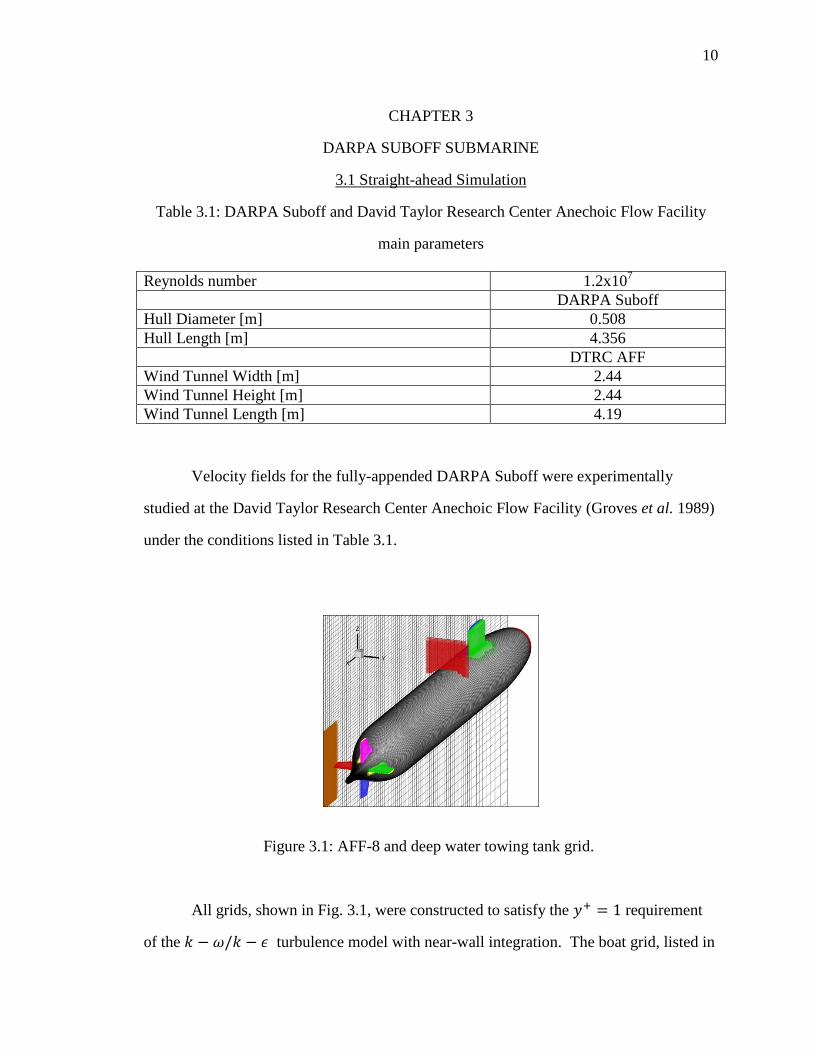
Velocity fields for the fully-appended DARPA Suboff were experimentally
studied at the David Taylor Research Center Anechoic Flow Facility (Groves et al. 1989)
under the conditions listed in Table 3.1.
Figure 3.1: AFF-8 and deep water towing tank grid.
All grids, shown in Fig. 3.1, were constructed to satisfy the requirement
of the turbulence model with near-wall integration. The boat grid, listed in
11
Table 3.2, consists of a hull grid (‘O’ type) and overlapping appendage grids intended to
provide a fine computational mesh for the wake. A Cartesian background grid is used to
impose wind tunnel boundaries, and two Cartesian refinement grids are used, one to
better capture the sail wake and the other grid to capture the wake of the boat. The
domain connectivity needed to perform overset computations was obtained using the
code Suggar (Noack, 2005) while surface overlap was pre-processed using Usurp (Boger
and Dreyer, 2006) to integrate the forces.
Table 3.2: Grid dimensions for AFF-8 submarine
Grid
Size
Total Points
Type
Hull 361x61x151 3.33 M ‘O‘
Nose 61x51x61 190 k Wrapped
Sail 2x61x51x121 2x376 k Wrapped
Rudders 4x61x51x61 4x190 k Wrapped
Stern Planes 4x61x51x61 4x190 k Wrapped
Refinement 1 351x109x101 3.86 M Cartesian
Refinement 2 277x205x205 11.6 M Cartesian
Background 187x109x109 2.22 M Cartesian
Total 23.5 M
A fourth-order biased scheme was used for convection for the momentum
equations with a second-order centered scheme used for diffusion and a second-order
backward discretization used in time. The turbulence equations used the same schemes
for diffusion and time but differed from the momentum equations by utilizing a second-
order upwind scheme for convection. The boundary conditions used were: no-slip for the
hull and appendages, imposed incoming velocity for the inlet, zero normal second
derivative for the exit, and farfield conditions for the tank.
Before computing self-propulsion a set of computations were performed for
DARPA Suboff towed in fully appended configuration without a propeller. These results

12
were compared against the data by Crook (1990), who measured the resistance in a deep
water towing tank. Figure 3.2 shows that the resistance predicted by RANS and DDES
computations is very close to the experimental values, and that DDES shows accurate
predictions for a wide range of speeds.
Figure 3.2: Resistance of Suboff Model 5470.
RANS and DDES were used to simulate the submarine moving straight ahead.
The wake was analyzed at the location for both simulations and the
experimental cases and shown in Fig 3.3. The hole in the center of each wake profile is
due to the trailing edge of the submarine and this testing void was duplicated for all
locations. The overall pattern of each wake is very similar, with reduced flow velocity
downstream of the appendages. Notice the high velocity observed in the wake of the sail,
where necklace vortices deplete the boundary layer at the center and send low-
momentum flow to the sides, causing a “V” shaped high-speed carving in the wake.
0
100
200
300
400
500
600
700
800
900
0.0 3.0 6.0 9.0 12.0 15.0 18.0 21.0
Res
ista
nce
[N
]
Model speed [Knots]
EFD (Crook 1990)EFD_BlockedCFD DDESCFD RANS

13
Figure 3.3: AFF-8 wake at .
The circumferentially averaged velocity is shown in Fig. 3.4 for RANS, DDES,
and EFD. The average velocity was found by creating a 360 node circular grid, one
degree separation between each node, and interpolating the RANS solution at each of
those locations. This procedure was repeated all radii and also for DDES and EFD
solutions. The two numerical simulations predicted almost the same value at large radii
(larger than ) but are a higher velocity than EFD. The largest difference occurs
at where the RANS velocity is 3.85% higher than experimental and the DDES
velocity is 3.95% higher. RANS begins to underpredict the velocity near the hull,
ultimately yielding a -12.9% error at compared to the 2.13% experienced by
DDES at that same radius.

14
Figure 3.4: AFF-8 circumferentially averaged velocity at .
Figure 3.5: AFF-8 shear stress at .
0
0.4
0.8
1.2
1.6
2
0.4 0.5 0.6 0.7 0.8 0.9 1.0
No
rmal
ized
Rad
ius
[-]
Normalized Velocity [-]
EFD Baseline and AppendagesCFD RANSCFD DDES
0
0.2
0.4
0.6
0.8
1
1.2
0.25 0.75 1.25 1.75
Shea
r St
ress
[m
Pa]
Normalized Radius [-]
EFDDDESRANS

15
The shear stress is shown in Fig. 3.5 for RANS, DDES, and EFD. With the
exception of the first and last radius, the stress predicted by RANS is always lower than
the measured experimental value. DDES predictions are closer to experimental than
RANS with most of the data points being within 5% of the measured values.
Figure 3.6: AFF-8 wake at .
Figure 3.7: AFF-8 wake at .
The wake profile was similarly evaluated downstream as previously done for
. Figure 3.6 and 3.7 show the wake at and . The
wake pattern is in good agreement with experiments. As expected, RANS predicts a more
16
diffused wake, while DDES tends to overpredict the effects of the sail on the flow field
causing a sharp contrast between the high speed flow immediately trailing the sail and the
low speed necklace wake. The wake shows a predictable trend as the flow becomes more
uniform farther away from the boundary layer effects of the submarine.
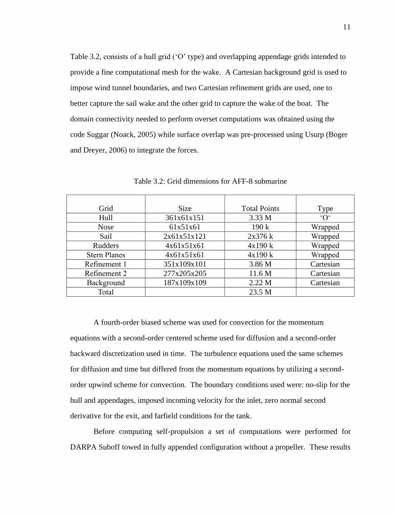
Figure 3.8 shows the submarine as it travels straight-ahead in the CFD DDES
simulation. The hull of the boat is colored by pressure while the slices are colored by
axial velocity. The wake development details can be observed as the boundary layer gets
thinner immediately downstream of the sail and thicker on the sides of this depleted area.
Figure 3.8: View of the DARPA Suboff submarine in straight-ahead case.

17
3.2 Turning Simulation
Table 3.3: DARPA Suboff fully-appended turning case main parameters.
Reynolds number 6.53x10⁶
Velocity [knots] 3
Rudder Angle [o] - 10
[o] 8.2
The Suboff submarine was experimentally tested completing a starboard turn with
a drift angle ( ) ranging between and for the bare hull and a single test of
for the fully-appended model. The steady turning experiments were performed
at Naval Surface Warfare Center Carderock Division in the Rotating Arm Basin. Static
pressure along the hull surface was measured with twenty-three pressure taps at each
location, and . Stereo PIV was used at the same axial locations
as the pressure measurements to capture the wake during the turn. The fully appended
simulation shown in Fig 3.9 was initialized in the middle of the turn, rotating
for with a and the parameters are listed in Table 3.3.
Figure 3.9: Rotating arm submarine turning case.

18
The turning case grids, found in Table 3.4, were constructed in the same manner
as was described in the straight-ahead simulation with a few minor changes. The hull
grid density was increased, as was the density on the rudders and stern planes. The
density of the refinement grid trailing the sail was also increased and the grid direction
reoriented, whereas the secondary refinement grid was coarsened for a total grid increase
of 2.9 M nodes.
Table 3.4: Grid dimensions for AFF-8 submarine turning case.
Grid
Size
Total Points
Type
Hull 481x101x241 11.7 M ‘O‘
Nose 61x51x61 190 k Wrapped
Sail 2x61x51x121 2x376 k Wrapped
Rudders 4x61x51x121 4x376 k Wrapped
Stern Planes 4x61x51x121 4x376 k Wrapped
Propeller Hub 101x37x101 377 k ‘O’
Refinement Gaps for Appendages 4x84x87x26 4x190 k Curvilinear Block
Refinement Sail Wake 386x121x111 5.18 M Cartesian
Refinement Wake 187x109x109 2.22 M Cartesian
Background 187x109x109 2.22 M Cartesian
Total 26.4 M
Figure 3.10 shows the submarine as it travels in the CFD rotating arm simulation.
The hull of the boat is colored by pressure while the slices are colored by total velocity to
display the boundary layer. The vortical structures, also colored by total velocity, are
shown as isosurfaces of . It is noticeable the effect of the necklace vortex on the
boundary layer, causing again a boundary layer depletion that the cross flow from the
rotation transports to starboard. The sail tip vortex rolls the low velocity wake flow from
the sail. The rudders produce significant tip vortices, indicating that under these
conditions the incoming flow angle of attack is large. The necklace vortices from the
rudders are very strong and become unstable, forming braided vortical wakes.

19
Figure 3.10: View of the DARPA Suboff submarine in rotating arm turn.
Figure 3.11: Turn velocity at .
The wake at was compared to the straight-ahead case to analyze
how the flow was change by the turning motion in Fig 3.11. The turning case exhibits an
almost horizontally symmetrical flow field with small influences from the sail. A vortex
20
from the tip of the port side stern plane is noticeable, although there is only marginal flow
impact from the rest of the stern plane. The effect of the other stern plane is lost among
the strong wake created by the drifting hull. The drifting hull is also largely responsible
for the large flow disturbance caused by the rudders, including the tip vortices seen at the
top and bottom of the frame.
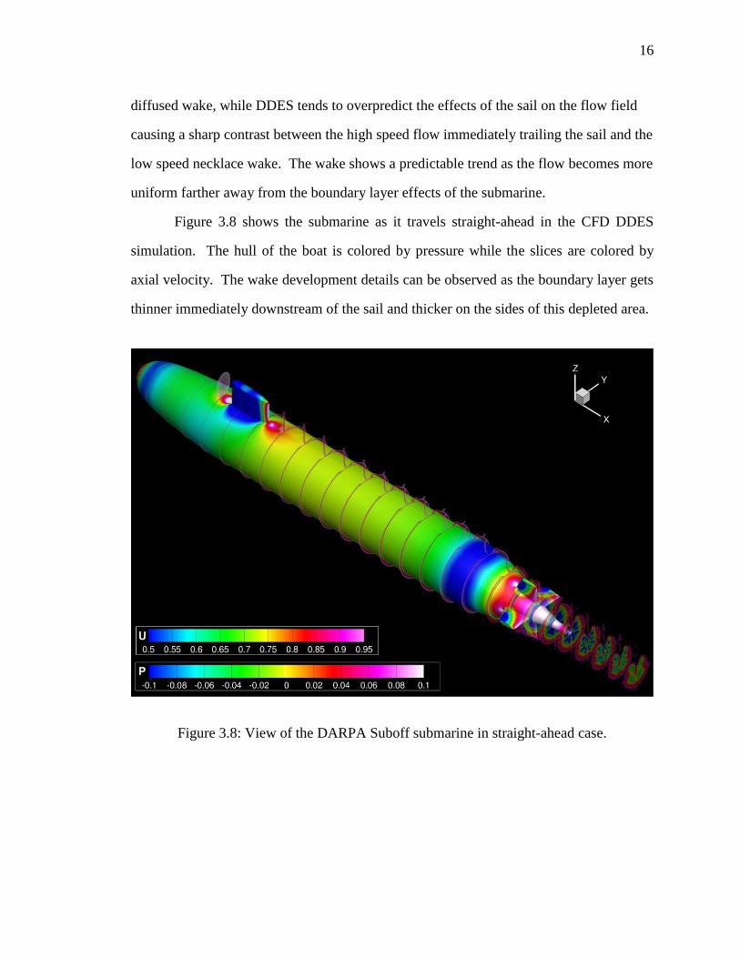
The vorticity found in the PIV experiment was compared to the CFD result at
in Fig 3.12. Color was omitted for vorticity values between -15 and 15 to
match the format of the experimental results (Atsavapranee 2010). The experimental axis
scales were also duplicated for proper comparison. There is good agreement between
CFD and experiments for the magnitude and location of the vorticity caused by the hull.
The sail tip vortex is also very well predicted, both in location and magnitude.
Figure 3.12: Turn velocity vectors and vorticity at .
Vorticity was also compared at , shown in Fig. 3.13, with CFD and
PIV in good agreement even though the drift angle in the experiment is 9% larger. While
the trends and magnitudes of vorticity are similar for both cases, CFD tends to diffuse the
vortical structures as evidenced by the less concentrated intensity in the sail tip vortex.

21
Figure 3.13: Turn velocity vectors and vorticity at .

22
CHAPTER 4
INSEAN E1619 PROPELLER
4.1. Geometry and Simulation Conditions
Table 4.1: INSEAN E1619 main propeller parameters
INSEAN E1619
Number of blades 7
Diameter [mm] 485
Hub Diameter Ratio 0.226
Pitch at r = 0.7 R 1.15
Chord at 0.75 R [mm] 6.8
The geometry of interest is the E1619 propeller, a seven bladed design by
INSEAN shown in Fig. 4.1. The propeller used in the experiments was created from one
single piece of avional aluminum alloy with a black anodized outer skin (Di Felice et al.
2009). The propeller’s main parameters are shown in Table 4.1. Open water
experiments were performed in the INSEAN towing tank, and wake velocity
measurements were made with LDV in a closed test loop.
Figure 4.1: Coarse grid system.
The overset grid system, shown in Fig. 4.1, was designed to rotate as a rigid body
in the Earth system of coordinates. All grids were constructed to satisfy the

23
requirement of the turbulence model with near-wall integration. Each
blade consists of a blade grid (‘O’ type) and a tip grid intended to close the blade and
provide a fine computational mesh for the tip vortices. The blade grids overlap with an
‘O’ shaft grid that contains the hub and the shaft profile. A Cartesian background grid is
used to impose the far-field, inlet and exit boundary conditions, and a Cartesian
refinement grid is used to better capture the wake of the propeller. The code Suggar
(Noack, 2005) was used to obtain the domain connectivity needed to perform overset
computations. To integrate the forces the surface overlap was pre-processed using Usurp
(Boger and Dreyer, 2006).
A grid for the shaft and hub alone was constructed by removing the blades from
the grids in Table 4.2, and used to correct the propeller thrust and torque by subtracting
the shaft/hub forces from the full grid forces, as done in the experiments. These
corrections are very minor.
For the momentum equations and all runs a fourth-order biased scheme was used
for convection, a second-order centered scheme was used for diffusion and a second-
order backward discretization was used in time. The same was used for the turbulence
equations but with a second-order upwind scheme for convection. No-slip boundary
conditions were used for the shaft, hub and blades, imposed incoming velocity for the
inlet, zero normal second derivative for the exit, and farfield conditions for the side of the
domain.

24
Table 4.2: Dimensions for grids used for verification study
Grid
Size
(Coarse, Medium,
Fine, Very Fine)
Total Points
(Coarse, Medium,
Fine, Very Fine)
Type
Shaft
159x29x80
201x37x101
253x46x127
318x57x159
369 k
751 k
1.48 M
2.88 M
‘O‘
Blades (1-7)
7x80x29x80
7x101x37x101
7x127x46x127
7x159x57x159
7x186 k
7x377 k
7x742 k
7x1.44 M
‘O‘
Tips (1-7)
7x48x40x48
7x61x51x61
7x76x64x76
7x95x80x95
7x92.2 k
7x190 k
7x370 k
7x722 k
Wrapped
Refinement
191x175x175
241x221x221
303x278x278
381x350x350
5.85 M
11.8 M
23.4 M
46.7 M
Cartesian
Background
148x86x86
187x109x109
235x137x137
295x172x172
1.09 M
2.22 M
4.41 M
8.73 M
Cartesian
Total
9.26 M
18.7 M
37.1 M
73.4 M
For the grid convergence study, four grids (coarse, medium, fine and very fine)
were generated. A grid coarsening factor of √ was applied in each direction with a
trilinear interpolation algorithm to the very fine grid to obtain the fine grid so that each
grid shape and point distribution would be as close to the source grid as possible. This
procedure was then repeated to create the medium and coarse grids. Details of the grids
are summarized in Table 4.2.

25
Figure 4.2: Wake grid system.
An additional grid was constructed to better capture the wake. The wake grid,
shown in Fig. 4.2, was created by taking the medium grid and adding a very fine
refinement block immediately downstream of the propeller blades. This block was added
to calculate the wake and tip vortices with much better accuracy than it was possible with
the previous grid system. The refinement grid added to the wake matches the grid size of
the fine grids used for the tips of the blades, thus providing a grid of consistent
refinement for the tip vortices in the wake. The wake grid is summarized in Table 4.3.
Table 4.3: Details of the wake grid
Grid
Size
Total Points
Type
Shaft 201x37x101 751 k ‘O‘
Blades (1-7) 7x101x37x101 7x377 k ‘O‘
Tips (1-7) 7x61x51x61 7x190 k Wrapped
Refinement 1 361x386x386 53.8 M Cartesian
Refinement 2 241x221x221 11.8 M Cartesian
Background 187x109x109 2.22 M Cartesian
Total 72.5 M

26
4.2. Verification and Validation
A grid convergence study was performed at using DDES. The
convergence histories of the thrust coefficient and torque coefficient for all grids
are shown in Figs. 4.3 and 4.4, respectively. The time step, , was
nondimensionalized using the last calculated time step of each specific simulation. These
figures show that the thrust and torque converge in time and that as the grid is refined
both and tend to converge to smaller values, with faster convergence for .
Figure 4.3: Convergence history of the thrust coefficient for different grids.

27
Figure 4.4: Convergence history of the torque coefficient for different grids.
Figure 4.5: Grid and time step convergence.

28
The grid and time step convergence results are shown in Fig. 4.5 with , , and
being nondimensionalized as , , and , respectively.
Three different time steps were used for the fine grid: fine ( ), medium ( ), and
coarse ( ) where (240 time steps per propeller revolution). The very
fine grid simulations under predict the torque and thrust by 1% and 5% respectively,
resulting in an overprediction of the efficiency of 4%. While these errors respect to the
experimental values are small and consistent with other CFD for propellers, the reasons
for the discrepancies are unknown.
The uncertainty analysis was done using the procedures described in (Stern et al.
2001a, 2001b) to estimate the grid and time step errors for , , and . The iterative
convergence error was neglected as every time step was reasonably converged for all the
variables. Table 4.4 shows the grid size and time step uncertainties for the three variables
and the two groups of three grids. The overall numerical uncertainty was estimated using
the group containing the very fine grid.
Table 4.4: Numerical uncertainty from grid and time step convergence for
KT 10 KQ
Grid Uncertainty (Coarse, Medium, and Fine
grids) ± 0.0033 ± 0.0111 ± 0.0086
Grid Uncertainty (Medium, Fine, and Very
Fine grids) ± 0.0004 ± 0.0019 ± 0.0053
Time Step Uncertainty ± 0.0450 ± 0.0128 ± 0.0017
CFD Result and Overall Numerical
Uncertainty
0.251±
0.045
0.465±
0.017
0.611±
0.009
4.3. Open Water Curve
The OWC was created by simulating the fine propeller grid at six different
advance coefficients and the wake grid at seven different coefficients. Comparison with
the experimental results is shown in Fig. 4.6, where the lines show the experimental

29
results. The numerical results for both grids are in excellent agreement with the data, but
slightly under predict thrust and torque at high propeller loads (low J) and overpredict at
lower loads (high J). Besides possible limitations with the computational method, these
differences between CFD and experiments could be caused by a variety of factors, among
them errors arising from differences in the geometry or the presence of the driving
mechanism for the shaft in the towing tank, which was neglected in the CFD
computations.
Figure 4.6: E1619 OWC for wake and fine grids.
The magnitude of the differences shown in Fig. 4.6 between CFD and
experiments are consistent with other computations of open water curves for surface ship
propellers (Rhee and Joshi 2005, Castro et al. 2011) and submarine propellers (Di Felice
et al. 2009). This paper computed a wide range of loads ( ), while Di
Felice et al. (2009) limit their analysis to .

30
4.4. Wake Analysis
4.4.1 Grid Comparison
The effects of the grid refinement on the wake are shown in Fig. 4.7, which
displays isosurfaces of the second invariant of the rate of strain tensor at for
the four grids. Axial velocity is indicated by levels of grey. Tip vortex pairing can be
observed for the fine and very fine grids but is not resolved by the coarser grids as the
lack of refinement causes the vortices to dissipate before pairing can occur. The effect of
the grid refinement on the wake solution is much stronger than in the resulting forces and
moments, as seen in the previous section. The strong hub vortex is visible in all levels of
refinement with the details less pronounced in coarser grids.
Figure 4.7: isosurfaces at for grids using DDES.

31
The total vorticity at the plane is shown in Fig. 4.8. Though the general
vorticity patterns are similar for all grids, diffusion and loss of vorticity are dramatic for
the coarser grids. Vortex pairing is evident in the fine and very fine grids as the co-
rotating tip vortices merge downstream of the propeller. This phenomenon was first
reported by Felli et al. (2011), and is more likely occur with tip vortices closer to each
other. The tip vortices are closer to each other at higher loads (low ) and for propellers
with more blades.
Figure 4.8: Vorticity for all grids at using DDES.
4.4.2 Wake Grid
At this point the computations are performed using the wake grid, which provides
a finer refinement in the wake region and thus suffers less from numerical diffusion than
the very fine grid. One high-load advance coefficient ( ) that presents significant
tip vortex interaction and was therefore computed with three turbulence approaches

32
(RANS, DES, DDES) and with no turbulence model to evaluate the effect of the
resolved/unresolved turbulence on the wake and the vortex pairing process.
Vortical structures for the four different solutions are shown in Fig. 4.9, displayed
as isosurfaces of greyscaled with axial velocity. For all cases the vortical
structures are observed until the end of the refinement grid, where the mesh resolution
becomes too coarse and the vortices are lost to diffusion.
Figure 4.9: isosurfaces for different turbulence models at .
Figure 4.10 shows the total vorticity at cross sections at the plane for the
four solution approaches. The with no turbulence model solution has only molecular
viscosity and is only subject to the small numerical diffusivity caused by the fourth-order
biased scheme (Ismail et al. 2010). As expected, the RANS solution overly dissipates the
tip vortices through an excess of modeled turbulent viscosity. The DES approach solves
the RANS problem of excessive diffusion by transitioning from RANS to LES in well

33
resolved grid regions, but usually tends to over-predict separation (Spalart 2009). This
problem is solved in many cases by DDES (Spalart 2009). Notice in Fig. 4.9 that the
solution with no turbulence model tends to show early instability of the tip vortices and
much more intense vorticity near the hub where necklace and trailing edge vortices are
strong. The DES and DDES solutions are similar, though DES predicts slightly stronger
vortices and thus a bit earlier pairing. The DDES solutions look more consistent with the
observations of tip vortices and pairing by Felli et al. (2011), and thus the method is
chosen for the following discussions.
Figure 4.10: Vorticity for different turbulence models at .
The efficiency along with the torque and thrust coefficients were calculated for
each method and the resulting values compared to the measured experimental values in
Table 4.5. As shown in Fig. 4.6 and Table 4.5, both thrust and torque are under-predicted
with CFD by about 7.8% and 5.9%, respectively, but the efficiency shows much smaller

34
error. The computations with no turbulence model yielded the results closest to the
experimental values with a difference in efficiency of 0.63%, while the RANS solution
was the least accurate with a difference in efficiency of 2.29%. DDES (1.74%) proved to
be slightly more accurate than DES (1.81%), although the variance was very small.
Table 4.5: Different solver methods at
KT 10 KQ
Experimental 0.4095 0.6226 0.4175
DDES 0.3777 0.5861 0.4103
RANS 0.3740 0.5835 0.4080
No turbulence model 0.3821 0.5863 0.4149
DES 0.3772 0.5857 0.4100
Figure 4.11: Q isosurfaces for all J's using DDES with the wake grid.
Isosurfaces of Q greyscaled with axial velocity for the six different advance
coefficients computed are shown in Fig. 4.11. The Q value and axial velocity range were

35
altered at each J value to match the corresponding propeller induced velocity, much
higher at lower J’s. Vortex pairing can be observed for all J’s lower than and is
delayed further downstream as the advance coefficient increases. As expected, the CFD
simulations correctly predict that the strength of the tip vortices decreases as the load
decreases.
Vorticity slices were taken for the six advance coefficients using the method
previously described and are shown in Fig. 4.12. At higher loads it is shown that the tip
vortices merge very quickly, initially in pairs of contiguous vortices, which results first in
three merged pairs and a free tip vortex, then these vortices merge in pairs forming two
stronger vortices, and ultimately these two also merge forming one large vortex at
.
Figure 4.12: Vorticity at different J's using DDES with the wake grid.

36
The phenomenon of helical vortex instability was numerically studied for wind
turbine rotors by Ivanell et al. (2010), who found pairing occurred several rotor radii
downstream of the hub for their conditions. Felli et al. (2011) observed that closer tip
vortices resulted in faster induction pairing. To reduce the distance between vortices and
study pairing the authors used higher advance coefficient for the same propeller geometry
or larger number of blades for the same advance coefficient. These two mechanisms in a
marine propeller lead to larger induced wake velocities and thus larger contraction of the
wake, favoring stronger mutual vortex induction and pairing over expanding wakes as is
the case of a wind turbine rotor.
Figure 4.13: Propeller velocity for at (data from Liefvendahl et al.
2010).
Figure 4.13 shows computed and experimental normalized axial velocity at
downstream of the propeller plane for , where R is the radius of the
propeller. The computations were performed with DDES on the wake grid, while the
experimental results were reported by Liefvendahl et al. (2010). The similarities between
CFD and experiments are remarkable, including the maximum velocity in the wake of the

37
blades, the velocity deficit induced by the tip vortices, and the acceleration around the
low velocity region in the trailing edge of the blades.

38
CHAPTER 5
SELF-PROPULSION
5.1. Simulation Conditions
Table 5.1: DARPA Suboff self-propelled by INSEAN E1619 main parameters
Reynolds number 1.2x10⁷
DARPA Suboff
Hull Diameter [m] 0.508
Hull Length [m] 4.356
INSEAN E1619
Propeller diameter [m] 0.262
A simulation of the DARPA Suboff fitted with the E1619 propeller under self-
propelled conditions was performed using DDES and the methodology described in
Carrica et al. (2010). Geometric details are similar to those used by Liefvendahl et al.
(2010), and are shown in Table 5.1. The grid is composed of overset blocks to build the
hull, sail, rudders, stern planes, and propeller. The assembly of individual meshes is
highlighted in Fig. 5.1, using different colors to denote each grid.
Figure 5.1: Grid for self-propelled submarine computations.

39
Table 5.2: Grid dimensions for self-propelled grid
Grid
Size
Total Points
Type
Hull 481x101x241 11.7 M ‘O‘
Nose 61x51x61 190 k Wrapped
Sail 2x61x51x121 2x376 k Wrapped
Rudders 4x61x51x121 4x376 k Wrapped
Stern Planes 4x61x51x121 4x376 k Wrapped
Propeller Hub 101x37x101 377 k ‘O’
Blades 7x101x37x101 7x377 k ‘O’
Tips 7x61x51x61 7x190 k Wrapped
Refinement Gaps for Appendages 4x84x87x26 4x190 k Curvilinear Block
Refinement Wake 241x221x221 11.8 M Cartesian
Refinement Wake 119x79x79 743 k Cartesian
Background 187x109x109 2.22 M Cartesian
Total 38.5 M
The grid dimensions for the self-propelled submarine are shown in Table 5.2.
The blade and tip grids around the propeller are the same as the medium grid from the
grid study. The grids that make up the propeller rotate as a child of the submarine. The
submarine and all related grids can move forward in surge, resulting in a computation in
an Earth-fixed inertial coordinate system. The computations for the self-propulsion case
use the same time step and reference values for length and velocity as the propeller open-
water curve case. A PI controller as described in Eq. (17) was used to modify the
rotational speed of the propeller, and to speed up the computation the inertia of the
submarine was reduced by a factor of 10, resulting in faster acceleration but in the same
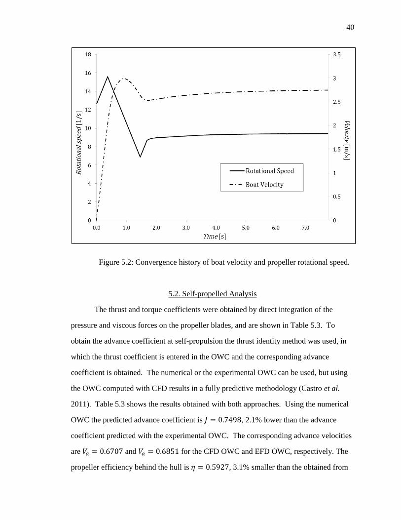
steady-state self-propulsion result. Convergence of the propeller rotational speed and boat
speed during the self-propulsion computation is shown in Fig. 5.2.
40
Figure 5.2: Convergence history of boat velocity and propeller rotational speed.
5.2. Self-propelled Analysis
The thrust and torque coefficients were obtained by direct integration of the
pressure and viscous forces on the propeller blades, and are shown in Table 5.3. To
obtain the advance coefficient at self-propulsion the thrust identity method was used, in
which the thrust coefficient is entered in the OWC and the corresponding advance
coefficient is obtained. The numerical or the experimental OWC can be used, but using
the OWC computed with CFD results in a fully predictive methodology (Castro et al.
2011). Table 5.3 shows the results obtained with both approaches. Using the numerical
OWC the predicted advance coefficient is , 2.1% lower than the advance
coefficient predicted with the experimental OWC. The corresponding advance velocities
are and for the CFD OWC and EFD OWC, respectively. The
propeller efficiency behind the hull is , 3.1% smaller than the obtained from

41
the OWC at the same operating point. These results are very close to those reported by
Liefvendahl and Tröeng (2011) for their computations of Suboff using a LES method.
Table 5.3: Self-propelled solution at m/s
KT
10 KQ
(CFD or OWC)
(CFD or OWC) J Va
Self-Propelled 0.2342 0.4714 0.5927 - -
Using CFD OWC 0.2342 0.4577 0.6115 0.7498 0.6707
Using Experimental OWC 0.2342 0.4353 0.6602 0.7659 0.6851
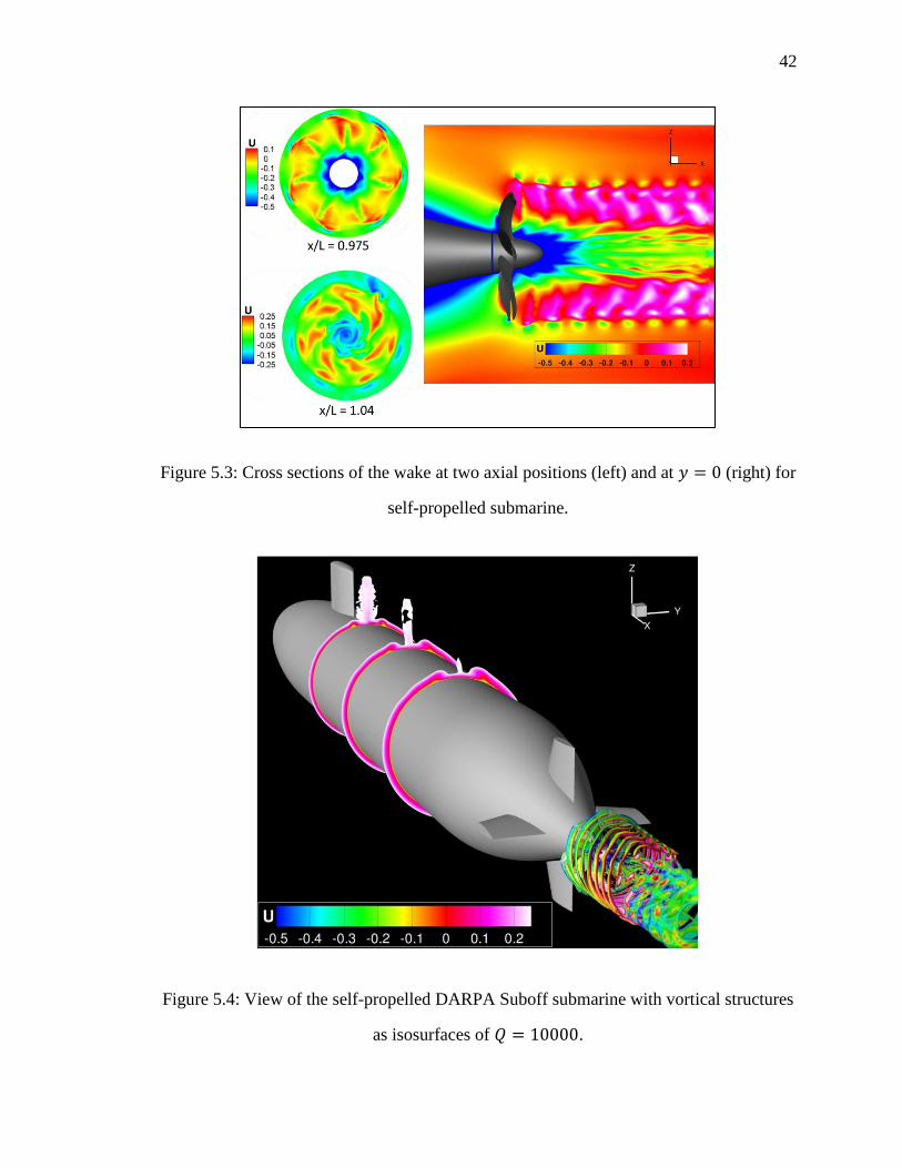
Cross-sectional cuts showing the instantaneous axial velocity at two different
axial planes behind the propeller can be found in Fig. 5.3, along with a cross section at
the plane . The far-field velocity for this computation is , since the
simulation is performed in an Earth-fixed coordinate system. The slice at is
comparable to the slice shown in Fig. 4.13. Notice the effect of the wake of the
submarine, which results in lower velocity behind the propeller closer to the hub, and
consequently higher load. At approximately 40 degrees from the top the wake of the sail
can be observed as a low velocity section and a stronger tip vortex due to the increased
load and leakage. At the effect of the sail is more noticeable and the induced
rotation inside the propeller wake has caused a significant distortion of the original flow
field. The decreasing radius of the wake as the flow accelerates behind the propeller is
evident, induced by both the propeller and the convergence of the flow behind the hull.
42
Figure 5.3: Cross sections of the wake at two axial positions (left) and at (right) for
self-propelled submarine.
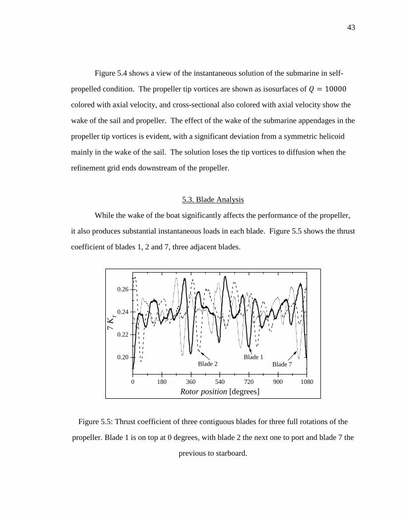
Figure 5.4: View of the self-propelled DARPA Suboff submarine with vortical structures
as isosurfaces of .
43
Figure 5.4 shows a view of the instantaneous solution of the submarine in self-
propelled condition. The propeller tip vortices are shown as isosurfaces of
colored with axial velocity, and cross-sectional also colored with axial velocity show the
wake of the sail and propeller. The effect of the wake of the submarine appendages in the
propeller tip vortices is evident, with a significant deviation from a symmetric helicoid
mainly in the wake of the sail. The solution loses the tip vortices to diffusion when the
refinement grid ends downstream of the propeller.
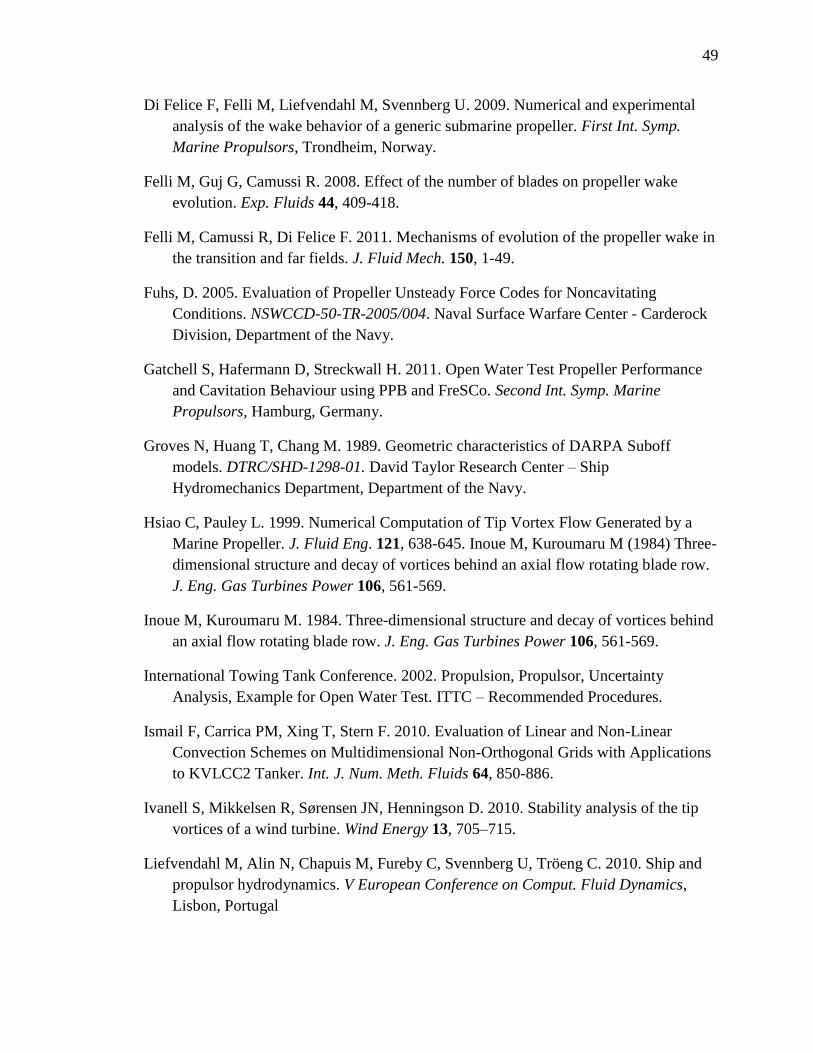
5.3. Blade Analysis
While the wake of the boat significantly affects the performance of the propeller,
it also produces substantial instantaneous loads in each blade. Figure 5.5 shows the thrust
coefficient of blades 1, 2 and 7, three adjacent blades.
Figure 5.5: Thrust coefficient of three contiguous blades for three full rotations of the
propeller. Blade 1 is on top at 0 degrees, with blade 2 the next one to port and blade 7 the
previous to starboard.
0 180 360 540 720 900 1080
0.20
0.22
0.24
0.26
Blade 2 Blade 7
7 K
T
Rotor position [degrees]
Blade 1

44
Blade 1 is on top at 0 degree rotation of the propeller, while blades 2 and 7 are
51.43 degrees to port and starboard, respectively. Notice in Fig. 5.5 that the peak to peak
fluctuations in thrust reach about 34% of the average thrust coefficient. The minimum
thrust occurs when the blades go through the top crossing the wake of the sail and the
maximum immediately before, which occurs approximately 40 degrees to port in this
right-handed propeller (angle in Fig. 5.5 increases clockwise looking at the propeller
from the stern).
The minimum thrust is due to the wake of the high speed downstream of the sail
caused by the boundary layer thinning resulting from the action of the necklace vortex
created by the sail, see Fig. 5.4. The wake in an axial plane upstream of the
propeller, presented in Fig. 5.6, shows the high axial speed region on top, and also the
low axial speed wake around it caused by the same necklace vortices. In these low speed
regions the load on the blades increases due to a locally lower advance velocity and
resulting higher effective angle of attack. Figure 5.6 also shows significant fluctuations
around this general behavior for different revolutions, though less energetic than those
predicted by Liefvendahl and Tröeng (2011) with their LES computations. The wake of
the rudders and stern planes are clearly visible, though relatively weak. Strong unsteady
vortices are present at about 120 and 160 degrees, and cause unsteady peaks in blade
thrust. These vortices are also necklace type and originated in the root of the rudders and
stern planes.

45
Figure 5.6: Instantaneous wake at an axial location upstream of the propeller. Every
11th
vector is shown for clarity.

46
CHAPTER 6
CONCLUSIONS AND RECOMMENDATIONS FOR FUTURE WORK
6.1. Conclusions
Results of a CFD study of the DARPA Suboff generic submarine hull fitted with
sail, rudders, stern planes, and submarine propeller E1619 have been presented. The
CFD computations were performed with a Delayed Detached Eddy Simulation approach.
The CFD wake of the submarine was in good agreement with the experimental data but
tended to overpredict the turbulence caused by the appendages. A rotating arm
simulation of the boat showed large disturbances of the wake caused by the necklace
wake generated at the sail that could result in large load fluctuations on the propeller
blades.
The predicted propeller open water curves for the generic propeller E1619 are
close to the experimental data, but tend to underpredict thrust and torque at high loads
and overpredict for lower loads. The verification study, performed on four grids and
three time steps for , shows that the thrust, torque and efficiency converge faster
in grid than in time step, and also that the wake is much more affected by the grid
refinement than the forces and moments. The wake of the propeller was analyzed with a
grid specifically refined to capture the tip vortices. A study of different turbulence
models at shows that RANS overly dissipates the wake and that in the solution
with no turbulence model the tip vortices quickly become physically unstable. DES and
DDES provide similar results, with DES showing slightly more vortex mutual induction.
Tip vortex pairing, studied experimentally by Felli et al. (2011) was observed at high
loads, showing multiple vortices merging for . The agreement of CFD with
experiments on the near wake axial velocities for is excellent.
Self-propulsion computations of the DARPA Suboff generic submarine hull fitted
with sail, rudders, stern planes and the E1619 propeller were performed in model scale
and the resulting propeller performance analyzed for conditions similar to those used by

47
Liefvendahl et al. (2010). The thrust identity method was used to obtain an effective
advance coefficient and advance velocity, and to compare the operating efficiency with
the open water efficiency. The results show that the same methodology applied to
surface ships by Carrica et al. (2010) and Castro et al. (2011) can be used to compute
self-propulsion of submarines.
6.2. Recommendations for Future Work
Future work is focused on coupling CFDShip-Iowa V4.5 with the potential flow
propeller solver PUF-14, with the goal of realizing substantial time savings over
discretized propeller computations, while still accounting for inhomogeneous and
transient wakes. The coupled solver needs to be validated for the E1619 propeller using
the experimental results previously described. After validation, CFDShip/PUF could be
used with the Suboff submarine to estimate self-propulsion and compare with the
discretized propeller for different maneuvers. The coupled solver could also be used to
evaluate other submarines under self-propulsion.

48
REFERENCES
Alin N., Bensow R.E., Fureby C., Huuva T., and Svennberge U. 2010. “Current
Capabilities of DES and LES for Submarines at Straight Course,” J. Ship Research
54, pp. 184-196.
Atsavapranee P. 2010. “Experimental Measurements for CFD Validation of the Flow
about a Submarine Model (Suboff),” Submarine Hydrodyn. Working Group Meeting,
Bethesda, MD, USA.
Boger DA, Dreyer JJ. 2006. Prediction of hydrodynamic forces and moments for
underwater vehicles using overset grids. AIAA Paper 2006-1148, 44th
AIAA
Aerospace Sciences Meeting, Reno, NV, USA.
Bull, P. 1996. “The validation of CFD predictions of nominal wake for the SUBOFF
fully appended geometry,” Twenty-first Symposium on Naval Hydrodynamics.
Trondheim, Norway.
Califano A, Steen S. 2011. Numerical simulations of a fully submerged propeller subject
to ventilation. Ocean Eng. 38, 1582-1599.
Carrica PM, Wilson RV, Stern F. 2007a. An unsteady single-phase level set method for
viscous free surface flows. Int. J. Numer. Meth. Fluids 53, 229-256.
Carrica PM, Wilson RV, Noack RW, Stern F. 2007b. Ship motions using single-phase
level set with dynamic overset grids Comput. Fluids 36, 1415-1433.
Carrica PM, Castro AM, Stern F. 2010. Self-propulsion computations using a speed
controller and a discretized propeller with dynamic overset grids. J. Mar. Sci.
Technol. 15, 316-330.
Carrica PM, Fu H, Stern F. 2011. Computation of self-propulsion free to sink and trim
and of motions in head waves of the KRISO Container Ship (KCS) model. Appl.
Ocean Res. 33, 309-320.
Castro AM, Carrica PM, Stern F. 2011. Full scale self-propulsion computations using
discretized propeller for the KRISO container ship KCS. Comput. Fluids 51, 35-47.
Crook B. 1990. Resistance for DARPA Suboff as Represented by Model 5470. David
Taylor Research Center report DTRC/SHD-1298-07.
Denny S. 1968. Cavitation and open-water performance tests of a series of propellers
designed by lifting-surface methods. Naval Ship Research and Development Center
report 2878, Naval Ship Research and Development Center, Department of the
Navy.
49
Di Felice F, Felli M, Liefvendahl M, Svennberg U. 2009. Numerical and experimental
analysis of the wake behavior of a generic submarine propeller. First Int. Symp.
Marine Propulsors, Trondheim, Norway.
Felli M, Guj G, Camussi R. 2008. Effect of the number of blades on propeller wake
evolution. Exp. Fluids 44, 409-418.
Felli M, Camussi R, Di Felice F. 2011. Mechanisms of evolution of the propeller wake in
the transition and far fields. J. Fluid Mech. 150, 1-49.
Fuhs, D. 2005. Evaluation of Propeller Unsteady Force Codes for Noncavitating
Conditions. NSWCCD-50-TR-2005/004. Naval Surface Warfare Center - Carderock
Division, Department of the Navy.
Gatchell S, Hafermann D, Streckwall H. 2011. Open Water Test Propeller Performance
and Cavitation Behaviour using PPB and FreSCo. Second Int. Symp. Marine
Propulsors, Hamburg, Germany.
Groves N, Huang T, Chang M. 1989. Geometric characteristics of DARPA Suboff
models. DTRC/SHD-1298-01. David Taylor Research Center – Ship
Hydromechanics Department, Department of the Navy.
Hsiao C, Pauley L. 1999. Numerical Computation of Tip Vortex Flow Generated by a
Marine Propeller. J. Fluid Eng. 121, 638-645. Inoue M, Kuroumaru M (1984) Three-
dimensional structure and decay of vortices behind an axial flow rotating blade row.
J. Eng. Gas Turbines Power 106, 561-569.
Inoue M, Kuroumaru M. 1984. Three-dimensional structure and decay of vortices behind
an axial flow rotating blade row. J. Eng. Gas Turbines Power 106, 561-569.
International Towing Tank Conference. 2002. Propulsion, Propulsor, Uncertainty
Analysis, Example for Open Water Test. ITTC – Recommended Procedures.
Ismail F, Carrica PM, Xing T, Stern F. 2010. Evaluation of Linear and Non-Linear
Convection Schemes on Multidimensional Non-Orthogonal Grids with Applications
to KVLCC2 Tanker. Int. J. Num. Meth. Fluids 64, 850-886.
Ivanell S, Mikkelsen R, Sørensen JN, Henningson D. 2010. Stability analysis of the tip
vortices of a wind turbine. Wind Energy 13, 705–715.
Liefvendahl M, Alin N, Chapuis M, Fureby C, Svennberg U, Tröeng C. 2010. Ship and
propulsor hydrodynamics. V European Conference on Comput. Fluid Dynamics,
Lisbon, Portugal

50
Liefvendahl M, Tröeng C. 2011. Computation of cycle-to-cycle variation in blade load
for a submarine propeller using LES. Second Int. Symp. Marine Propulsors,
Hamburg, Germany.
Menter FR. 1994. 2-equation Eddy Viscosity Turbulence Models per Engineering
Applications. AIAA J. 32, 1598-1605.
Noack R. 2005. Suggar: a general capability for moving body overset grid assembly.
AIAA paper 2005-5117, 17th AIAA Computational Fluid Dynamics Conf., Toronto,
ON, Canada.
Rhee S, Joshi S. 2005. Computational Validation for Flow around a Marine Propeller
Using Unstructed Mesh Based Navier-Stokes Solver. JSME Int. J. 48, 562-570
Stern F, Wilson R, Coleman H, Paterson E. 2001a. Comprehensive approach to
verification and validation of CFD simulations—Part 1: Methodology and
procedures. J. Fluids Eng. 123, 793-802
Stern F, Wilson R, Coleman H, Paterson E. 2001b. Comprehensive approach to
verification and validation of CFD simulations—Part 2: Application for RANS
simulation of a cargo/container ship. J. Fluids Eng. 123, 803-810
Spalart P. 2009. Detached Eddy Simulation. Annu. Rev. Fluid Mech. 41, 181–202
Watanabe T, Kawamura T, Takekoshi Y, Maeda M, Rhee S. 2003. Simulation of steady
and unsteady cavitation on a marine propeller using a RANS CFD code. Fifth Int.
Symp. Cavitation, Osaka, Japan.
Xing T, Kandasamy M, Stern F. 2007. Unsteady free-surface wave-induced separation:
analysis of turbulent structures using detached eddy simulation and single-phase
level set. J. Turbulence 8, 1-35
Xing T, Carrica PM, Stern F. 2010. Large-scale RANS and DDES computations of
KVLCC2 at drift angle 0 degree. A Workshop on Numerical Ship Hydrodynamics,
Gothenburg, Sweden
Young Y, Kinnas S. 2003. Analysis of supercavitating and surface-piercing propeller
flows via BEM. Comput. Mech. 32, 269-280.
Yu-cun P, Huai-xin Z. 2010. Numerical Hydro-Acoustic Prediction of Marine Propeller
Noise. J. Shanghai Jiaotong Univ. (Sci.) 15, 707-712.