Parkland College

A with Honors Projects Honors Program

2012

Heat EquationWyatt SherlockParkland College

Open access to this Article is brought to you by Parkland College's institutional repository, SPARK: Scholarship at Parkland. For more information,please contact spark@parkland.edu.

Recommended CitationSherlock, Wyatt, "Heat Equation" (2012). A with Honors Projects. 52.http://spark.parkland.edu/ah/52

PARKLAND COLLEGE MATH 229

Heat Equation Derivation and Analytical Solution

Wyatt Sherlock Spring 2012

Abstract

This document describes the process of deriving the heat equation from known thermodynamic laws followed by an analytic solution. Towards the end of the document, the heat equation is discussed in terms of practical engineering problems.

Introduction

z

0 ≤ x ≤ L

x

y

0 a Δx b L

The cylinder above is a section of thin metal rod with insulation. The inner cylinder is the metal rod while the outer cylinder is rubber insulation. Let’s say that the insulation inhibits the flow of heat in the y and z directions so that the heat flows in the x direction only. Since the metal rod is very thin, this can be regarded as a one dimensional case. A very thin metal plate would be an example of a two dimensional case.

Deriving the Heat Equation in One Dimension

It is experimentally determined that

∆𝑄 = 𝑐𝜌𝑢(𝑥, 𝑡)∆𝑉

Where Q is the heat, c is the specific heat, 𝜌 is the density, u is the temperature as a function of x and t, and ∆𝑉 is a very small volume.

Since the rod is of a uniform diameter, the equation becomes

∆𝑄 = 𝑐𝜌𝑢(𝑥, 𝑡)𝐴∆𝑥

where A is the cross sectional surface area of the rod. If I integrate both sides from b to a, the equation becomes

∫ 𝑑𝑄 = ∫ 𝑐𝜌𝐴𝑢(𝑥, 𝑡)𝑑𝑥

𝑄(𝑡) = 𝑐𝜌𝐴𝑢(𝑥, 𝑡)𝑑𝑥𝑎

𝑏

where Q is a function of time. Differentiating and using Leibniz’s Rule

𝑑𝑄𝑑𝑡

=𝑑𝑑𝑡 𝑐𝜌𝐴𝑢(𝑥, 𝑡)𝑑𝑥 =𝑎

𝑏 𝑐𝜌𝐴

𝜕𝑢𝜕𝑡𝑑𝑥

𝑎

𝑏

Fourier’s Law states that heat will flow from hot regions to cold regions. Heat is proportional to the negative gradient of the temperature.

𝒒 = −𝑘𝐴𝛁𝑢

The rate of heat passing through the boundary at position a is given by

𝑑𝑄𝑑𝑡

= 𝑘𝐴𝛁𝑢(𝑥, 𝑡) ⋅ 𝒏𝑑𝑠𝑎

where n is the unit normal vector and ds is an infinitesimal surface at a. The Divergence Theorem in general is

𝑭 ⋅ 𝒏𝑑𝑠𝑆

= 𝛁 ⋅ 𝑭𝑑𝑉𝑄

F = 𝜵𝑢(𝑥, 𝑡)

n

a b

where S is a closed surface from a to b. Q is the small volume from a to b. Since the vector field (heat) is only flowing in the x direction, the theorem can be simplified.

𝑭 = 𝜵𝑢(𝑥, 𝑡) =𝜕𝑢𝜕𝑥

𝚤 +𝜕𝑢𝜕𝑦

𝚥+𝜕𝑢𝜕𝑧

𝑘 =𝜕𝑢𝜕𝑥

𝚤

The flux through the surface at a is

𝑭 ⋅ 𝒏𝑑𝑠 = 𝜕𝜕𝑥

𝚤 ⋅𝜕𝑢𝜕𝑥

𝚤𝑑𝑥𝑎

𝑏𝑎

𝑑𝑄𝑑𝑡

= 𝑘𝐴𝛁𝑢(𝑥, 𝑡) ⋅ 𝒏𝑑𝑠𝑎

= 𝑘𝐴𝜕𝜕𝑥

𝑎

𝑏𝜕𝑢𝜕𝑥𝑑𝑥

𝑑𝑄𝑑𝑡

= 𝑘𝐴 𝜕2𝑢𝜕𝑥2

𝑎

𝑏𝑑𝑥

𝑑𝑄𝑑𝑡

= 𝑐𝜌𝐴𝜕𝑢𝜕𝑡𝑑𝑥

𝑎

𝑏= 𝑘𝐴

𝜕2𝑢𝜕𝑥2

𝑎

𝑏𝑑𝑥

𝑐𝜌𝐴𝜕𝑢𝜕𝑡𝑑𝑥

𝑎

𝑏= 𝑘𝐴

𝜕2𝑢𝜕𝑥2

𝑎

𝑏𝑑𝑥

𝑐𝜌𝐴𝜕𝑢𝜕𝑡𝑑𝑥

𝑎

𝑏− 𝑘𝐴

𝜕2𝑢𝜕𝑥2

𝑎

𝑏𝑑𝑥 = 0

𝑐𝜌𝐴𝜕𝑢𝜕𝑡

− 𝑎

𝑏 𝑘𝐴

𝜕2𝑢𝜕𝑥2

𝑑𝑥 = 0

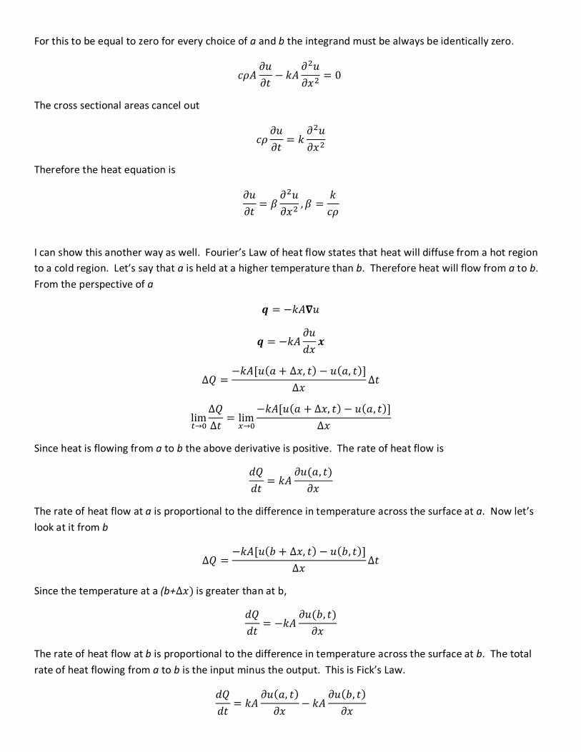
For this to be equal to zero for every choice of a and b the integrand must be always be identically zero.

𝑐𝜌𝐴𝜕𝑢𝜕𝑡

− 𝑘𝐴𝜕2𝑢𝜕𝑥2

= 0

The cross sectional areas cancel out

𝑐𝜌𝜕𝑢𝜕𝑡

= 𝑘𝜕2𝑢𝜕𝑥2

Therefore the heat equation is

𝜕𝑢𝜕𝑡

= 𝛽𝜕2𝑢𝜕𝑥2

,𝛽 =𝑘𝑐𝜌

I can show this another way as well. Fourier’s Law of heat flow states that heat will diffuse from a hot region to a cold region. Let’s say that a is held at a higher temperature than b. Therefore heat will flow from a to b. From the perspective of a

𝒒 = −𝑘𝐴𝛁𝑢

𝒒 = −𝑘𝐴𝜕𝑢𝑑𝑥

𝒙

∆𝑄 =−𝑘𝐴[𝑢(𝑎 + ∆𝑥, 𝑡) − 𝑢(𝑎, 𝑡)]

∆𝑥∆𝑡

lim𝑡→0

∆𝑄∆𝑡

= lim𝑥→0

−𝑘𝐴[𝑢(𝑎 + ∆𝑥, 𝑡) − 𝑢(𝑎, 𝑡)]∆𝑥

Since heat is flowing from a to b the above derivative is positive. The rate of heat flow is

𝑑𝑄𝑑𝑡

= 𝑘𝐴𝜕𝑢(𝑎, 𝑡)𝜕𝑥

The rate of heat flow at a is proportional to the difference in temperature across the surface at a. Now let’s look at it from b

∆𝑄 =−𝑘𝐴[𝑢(𝑏 + ∆𝑥, 𝑡) − 𝑢(𝑏, 𝑡)]

∆𝑥∆𝑡

Since the temperature at a (b+∆𝑥) is greater than at b,

𝑑𝑄𝑑𝑡

= −𝑘𝐴𝜕𝑢(𝑏, 𝑡)𝜕𝑥

The rate of heat flow at b is proportional to the difference in temperature across the surface at b. The total rate of heat flowing from a to b is the input minus the output. This is Fick’s Law.

𝑑𝑄𝑑𝑡

= 𝑘𝐴𝜕𝑢(𝑎, 𝑡)𝜕𝑥

− 𝑘𝐴𝜕𝑢(𝑏, 𝑡)𝜕𝑥

Using the Fundamental Theorem of Calculus

𝑑𝑄𝑑𝑡

= 𝑘𝐴𝜕𝜕𝑥

𝑎

𝑏

𝜕𝑢𝜕𝑥

𝑑𝑥

The result is the same

𝜕𝑢𝜕𝑡

= 𝛽𝜕2𝑢𝜕𝑥2

,𝛽 =𝑘𝑐𝜌

Solving the Heat Equation

β is called thermal diffusivity and it can vary depending on the type of material used. Let’s say that β is .05.

𝛽 = .05 m2

𝑠

I am going to set up some initial and boundary conditions for the heat equation. These can vary depending on the problem.

𝑢(𝑥, 0) = 0 0 < 𝑥 < 𝐿

𝑢(0, 𝑡) = 0

𝑢(𝐿, 𝑡) = 100, 𝐿 = 4m

𝜕𝑢𝜕𝑡

= 𝛽𝜕2𝑢𝜕𝑥2

So let’s say that the left end is submersed in a tank of boiling water kept at 100° C. The right end of the rod is in contact with a block of ice that is always kept at 0° C

100° C 0° C

The heat equation is linear. I can write the solution as a linear combination of two other solutions. The first solution I can find is the steady state solution. Steady state means that rate of heat flowing into the rod is equal to the rate of heat flowing out of the rod. So the rod is in a state of heat equilibrium. Fourier’s Law states that heat will diffuse from hot areas to cold areas. After a long amount of time the rod will be at heat equilibrium, the rate of heat flowing into and out of the rod is the same. As time t goes to infinity heat equilibrium will not change. So temperature becomes a function of x only. Therefore

𝜕𝑢𝐸𝜕𝑡

=𝜕2𝑢𝐸𝜕𝑥2

= 0,𝑢𝐸(0) = 0,𝑢𝐸(4) = 100

uE is the equilibrium temperature. Integrating twice produces

𝑢𝐸 = 𝐴𝑥 + 𝐵,𝑢𝐸(0) = 0,𝑢𝐸(4) = 100

So plugging in initial conditions I find that B is zero and A is 25.

𝑢𝐸(𝑥) = 𝑇𝑓 − 𝑇𝑖𝐿

𝑥 + 𝑇𝑖

𝑢𝐸(𝑥) = 100 − 0

4𝑥 + 0 = 25𝑥

Next I want to look at when heat is initially diffusing through the rod. Let’s define the function

𝑤(𝑥, 𝑡) = 𝑢(𝑥, 𝑡) − 𝑢𝐸(𝑥)

Where u is the solution to the heat equation and 𝑢𝐸 is the equilibrium condition. Let’s take the first and second derivatives with respect to t.

𝜕𝑤(𝑥, 𝑡)𝜕𝑡

=𝜕𝑢(𝑥, 𝑡)𝜕𝑡

−𝜕𝑢𝐸(𝑥)𝜕𝑡

𝜕2𝑤(𝑥, 𝑡)𝜕𝑡2

=𝜕2𝑢(𝑥, 𝑡)𝜕𝑡2

So u and w satisfy the same partial differential equation. Now I am going to plug in my initial and boundary conditions.

𝑤(𝑥, 0) = 𝑢(𝑥, 0) − 25𝑥 = 0 − 25𝑥 = −25𝑥

𝑤(0, 𝑡) = 𝑢(0, 𝑡) − 0 = 0

𝑤(4, 𝑡) = 𝑢(4, 𝑡) − 100 = 0

Now the boundary conditions are homogenous, therefore I can use separation of variables.

𝑤(𝑥, 𝑡) = 𝑋(𝑥)𝑇(𝑡)

Plugging back into the heat equation

𝑋(𝑥)𝑑𝑇(𝑡)𝑑𝑡

= 𝛽𝑇(𝑡)𝑑2𝑋(𝑥)𝑑𝑥2

Using prime notation

𝑇′

𝛽𝑇=𝑋′′

𝑋= −Ω

For whatever choice of t the right hand side must equal to a constant, Ω. The same goes whatever choice of x. From the assumption above, these two expressions must equal each other for whatever choice of x and t. Choosing omega to be negative is just for convenience.

𝑇′ + 𝛽Ω𝑇 = 0 [1]

𝑋′′ + Ω𝑋 = 0 [2]

These are two ordinary differential equations

Solving equation 1

𝑑𝑇𝑑𝑡

= −𝛽Ω𝑇

𝑑𝑇 = −𝛽Ω𝑇𝑑𝑡

𝑑𝑇 = −𝛽Ω𝑇𝑑𝑡

𝑇(𝑡) = 𝐶1𝑒−𝛽Ω𝑡

Solving equation 2

𝑋′′ + Ω𝑋 = 0

This is a homogeneous second order linear differential equation with constant coefficients. The solution for the differential equation will differ based on the value of Ω.

If Ω < 0

Ω = −ψ2

where ψ is some nonzero constant. I make this substitution because it avoids square roots.

𝑋′′ − ψ2𝑋 = 0

The characteristic polynomial is

𝑟2 − ψ2 = 0

𝑟 = ±ψ

𝑋(𝑥) = 𝐶2𝑒ψ𝑥 + 𝐶3𝑒−ψ𝑥

Plugging in initial conditions

𝑢(0, 𝑡) = 0 = 𝑢(𝐿, 𝑡)

0 = 𝐶2 + 𝐶3

𝐶2 = −𝐶3

0 = 𝐶2𝑒ψ𝐿 + 𝐶3𝑒−ψ𝐿

0 = 𝐶2(𝑒ψ𝐿 − 𝑒−ψ𝐿)

Ω is some constant ≠ 0 so then ψ is ≠ 0. Therefore 𝐶2 must be zero as well as 𝐶3.

𝑋(𝑥) = 0

This will produce a trivial solution.

Ω = 0 will produce a trivial solution as well.

Now let’s say that Ω > 0

Ω = ψ2

𝑋′′ + ψ2𝑋 = 0

The characteristic polynomial is

𝑟2 + ψ2 = 0

𝑟 = ±ψi

𝑋(𝑥) = 𝐶2𝑐𝑜𝑠𝜓𝑥 + 𝐶3𝑠𝑖𝑛𝜓𝑥

Plugging in initial conditions

𝑢(0, 𝑡) = 0 = 𝑢(𝐿, 𝑡)

𝐶2 = 0

0 = 𝐶3𝑠𝑖𝑛𝜓𝐿

The sine function is 0 when

𝜓𝐿 = 𝑛𝜋, 𝑛 = 0, 1, 2, 3, 4 …

As a result

𝑋(𝑥) = 𝑠𝑖𝑛𝑛𝜋𝑥𝐿

[1]

I can leave off the constant because it will be absorbed into a single constant at the end.

Ω𝑛 = ψ2 = 𝑛𝜋𝐿2

[2]

Equation 1 is the eigenfunction and equation 2 is the eigenvalue for the problem. Here I left off n = 0 because it produces zero for any choice of x. So

𝑛 = 1, 2, 3, 4 …

Hence there are infinitely many solutions to the spatial differential equation.

𝑋𝑛(𝑥) = 𝑠𝑖𝑛𝑛𝜋𝑥𝐿

The solution is

𝑤𝑛(𝑥, 𝑡) = 𝐶𝑛𝑠𝑖𝑛𝑛𝜋𝑥𝐿

𝑒−𝛽𝑛𝜋𝐿

2𝑡

I have found infinitely many solutions. The solution above satisfies the homogenous boundary conditions. The entire solution is the sum of all the eigenvalues and eigenfunctions. Cn will change for each value of n.

𝑤(𝑥, 𝑡) = 𝐶𝑛𝑠𝑖𝑛𝑛𝜋𝑥𝐿

𝑒−𝛽𝑛𝜋𝐿

2𝑡

∞

𝑛=1

At t = 0, the exponential factor equals one.

𝑤(𝑥) = 𝐶𝑛𝑠𝑖𝑛𝑛𝜋𝑥𝐿

∞

𝑛=1

= −25𝑥

𝐶𝑛𝑠𝑖𝑛𝑛𝜋𝑥𝐿

∞

𝑛=1

This is the Fourier sine series. Now I need to find the value of Cn.

First I am going to assume that w(x) is an odd function. This makes sense because sine is also an odd function. I am also going to assume that the series converges to w(x) on the interval –L ≤ x ≤ L. Next, I want to show that

𝑠𝑖𝑛𝑛𝜋𝑥𝐿

Is mutually orthogonal for n = 1,2,3,4…, on the interval –L ≤ x ≤ L and 0 ≤ x ≤ L. Two functions are said to be mutually orthogonal for m = 1,2,3,4…

𝑓(𝑥)𝑖𝑔(𝑥)𝑗𝑑𝑥 = 0, 𝑛 ≠ 𝑚𝜀 > 0, 𝑛 = 𝑚

𝑏

𝑎

Therefore

𝑠𝑖𝑛𝑛𝜋𝑥𝐿

𝐿

−𝐿𝑠𝑖𝑛

𝑚𝜋𝑥𝐿

𝑑𝑥 = 2 𝑠𝑖𝑛𝑛𝜋𝑥𝐿

𝑠𝑖𝑛𝑚𝜋𝑥𝐿

𝑑𝑥𝐿

0

This is true because two odd functions will produce an even function.

Now if n = m then the expression results in

2 𝑠𝑖𝑛𝑛𝜋𝑥𝐿

𝑠𝑖𝑛𝑚𝜋𝑥𝐿

𝑑𝑥𝐿

0= 2 𝑠𝑖𝑛2

𝑛𝜋𝑥𝐿

𝑑𝑥 = 1 − 𝑐𝑜𝑠2𝑛𝜋𝑥𝐿

𝑑𝑥 = 𝐿 − 𝑠𝑖𝑛2𝑛𝜋𝐿𝐿

×𝐿

2𝑛𝜋

𝐿

0

𝐿

0

Therefore

𝑠𝑖𝑛𝑛𝜋𝑥𝐿

𝐿

−𝐿𝑠𝑖𝑛

𝑚𝜋𝑥𝐿

𝑑𝑥 = 2 𝑠𝑖𝑛𝑛𝜋𝑥𝐿

𝑠𝑖𝑛𝑚𝜋𝑥𝐿

𝑑𝑥𝐿

0= 𝐿 𝑓𝑜𝑟 𝑎𝑙𝑙 𝑚 𝑎𝑛𝑑 𝑛 𝑤ℎ𝑒𝑛 𝑛 = 𝑚

Now if n ≠ m

𝑠𝑖𝑛𝑛𝜋𝑥𝐿

𝐿

−𝐿𝑠𝑖𝑛

𝑚𝜋𝑥𝐿

𝑑𝑥 = 2 𝑠𝑖𝑛𝑛𝜋𝑥𝐿

𝑠𝑖𝑛𝑚𝜋𝑥𝐿

𝑑𝑥𝐿

0

Using the trigonometric identity

𝑠𝑖𝑛𝐴𝑠𝑖𝑛𝐵 =12

[cos(𝐴 − 𝐵) − cos (𝐴 + 𝐵)]

2 𝑠𝑖𝑛𝑛𝜋𝑥𝐿

𝑠𝑖𝑛𝑚𝜋𝑥𝐿

𝑑𝑥𝐿

0= 𝑐𝑜𝑠

𝑛𝜋𝑥 − 𝑚𝜋𝑥𝐿

𝐿

0− 𝑐𝑜𝑠

𝑛𝜋𝑥+ 𝑚𝜋𝑥𝐿

𝑑𝑥

Therefore

𝑐𝑜𝑠𝑛𝜋𝑥 −𝑚𝜋𝑥

𝐿

𝐿

0− 𝑐𝑜𝑠

𝑛𝜋𝑥+ 𝑚𝜋𝑥𝐿

𝑑𝑥 = 𝑠𝑖𝑛 𝑛𝜋𝐿 −𝑚𝜋𝐿

𝐿×

𝐿𝜋(𝑛 −𝑚)− 𝑠𝑖𝑛

𝑛𝜋𝐿+ 𝑚𝜋𝐿𝐿

×𝐿

𝜋(𝑛+ 𝑚)

This becomes

𝑠𝑖𝑛(𝜋(𝑛 −𝑚)) ×𝐿

𝜋(𝑛 −𝑚)− 𝑠𝑖𝑛𝜋(𝑛 + 𝑚)×𝐿

𝜋(𝑛 +𝑚) = 0 𝑓𝑜𝑟 𝑎𝑙𝑙 𝑚 𝑎𝑛𝑑 𝑛 𝑤ℎ𝑒𝑛 𝑛 ≠ 𝑚

𝑠𝑖𝑛𝑛𝜋𝑥𝐿

𝐿

−𝐿𝑠𝑖𝑛

𝑚𝜋𝑥𝐿

𝑑𝑥 = 2 𝑠𝑖𝑛𝑛𝜋𝑥𝐿

𝑠𝑖𝑛𝑚𝜋𝑥𝐿

𝑑𝑥 = 0 𝐿

0

Now

𝑤(𝑥) = 𝐶𝑛𝑠𝑖𝑛𝑛𝜋𝑥𝐿

∞

𝑛=1

= −25𝑥

Multiplying both sides by

𝑠𝑖𝑛𝑚𝜋𝑥𝐿

Produces

𝑠𝑖𝑛𝑛𝜋𝑥𝐿

𝑤(𝑥) = 𝐶𝑛𝑠𝑖𝑛𝑛𝜋𝑥𝐿

𝑠𝑖𝑛𝑚𝜋𝑥𝐿

∞

𝑛=1

Then integrating

𝑠𝑖𝑛𝑛𝜋𝑥𝐿

𝑤(𝑥)𝑑𝑥 = 𝐶𝑛𝑠𝑖𝑛𝑛𝜋𝑥𝐿

𝑠𝑖𝑛𝑚𝜋𝑥𝐿

∞

𝑛=1

𝑑𝑥𝐿

−𝐿

𝐿

−𝐿

𝑠𝑖𝑛𝑛𝜋𝑥𝐿

𝑤(𝑥)𝑑𝑥 = 𝐶𝑛 𝑠𝑖𝑛𝑛𝜋𝑥𝐿

𝑠𝑖𝑛𝑚𝜋𝑥𝐿

𝑑𝑥𝐿

−𝐿

∞

𝑛=1

𝐿

−𝐿

Now the right hand side of the equation is always zero when n ≠ m. The equation below is true only when n = m. Therefore there will be one non-zero integral.

1𝐿 𝑠𝑖𝑛

𝑚𝜋𝑥𝐿

𝑤(𝑥)𝑑𝑥 =2𝐿 𝑠𝑖𝑛

𝑚𝜋𝑥𝐿

𝑤(𝑥)𝑑𝑥 =𝐿

0𝐶𝑚,𝑚 = 1,2,3,4 …

𝐿

−𝐿

So

2𝐿 𝑠𝑖𝑛

𝑛𝜋𝑥𝐿

𝑤(𝑥)𝑑𝑥 = 𝐶𝑛, 𝑛 = 1,2,3,4 …𝐿

0

𝐶𝑛 =24 𝑠𝑖𝑛

𝑛𝜋𝑥4

𝐿

0(−25𝑥)𝑑𝑥 = −

252 𝑥𝑠𝑖𝑛

𝑛𝜋𝑥4

4

0𝑑𝑥 = −

252

16(sin(𝑛𝜋)− 𝑛𝜋 cos(𝑛𝜋))𝑛2𝜋2

= −252−16𝑛𝜋(−1)𝑛

𝑛2𝜋2 =

200𝜋𝑛

(−1)𝑛

Sine is always zero for multiples of pi and cosine alternates between negative one and positive one.

So plugging everything back in, I get

𝑤(𝑥) = 200𝜋𝑛

(−1)𝑛𝑠𝑖𝑛𝑛𝜋𝑥𝐿

∞

𝑛=1

= −25𝑥

𝑤(𝑥, 𝑡) = 200𝜋𝑛

(−1)𝑛𝑠𝑖𝑛𝑛𝜋𝑥

4

∞

𝑛=1

𝑒−(.05)𝑛𝜋4 2𝑡

Therefore

𝑢(𝑥, 𝑡) = 25𝑥 + 200𝜋𝑛

(−1)𝑛𝑠𝑖𝑛𝑛𝜋𝑥

4

∞

𝑛=1

𝑒−(.05)𝑛𝜋4 2𝑡

As you can see this satisfies the initial condition and the steady state condition

At t = 0, u(x,t) = 0 because the sum converges to -25x for 0 < x < L. As t goes to ∞, u(x,t) approaches 25x

It also satifies the boundary conditions at x = 0, u(x,t) = 0 and at x = L = 4, u(x,t) = 100.

The following graph shows the preceeding expression plotted as a function of distance and time. As time goes to infinity, the temperature approaches the steady state condition.

Importance to Engineering

I showed how heat diffuses through a very thin metal rod. This is interpreted as temperature as a function of distance and time. This is not exclusively for thin metal rods, it can be used in two and three dimensions as well. Also boundary and initial conditions can change from example to example.

In the world of engineering, mechanical engineering in particular, this is very important. It allows for the modeling of heat transfer through an engine, for example. Different materials behave differently under high temperature conditions. An engine block machined out of cast iron will respond differently to heat transfer than an aluminum one. Choosing the right type of material is critical in engineering a car. Failure to do so may result in the melting of the engine.

One instance, the Chevrolet Vega had a cast aluminum engine block. This was ideal for fuel consumption and strength however problems with the coolant system ultimately led to engine distortion and failure. MG Midgets had a similar coolant system problem however Midget engine blocks were cast iron and could handle much higher temperatures.

The thermal diffusivity, β, of aluminum and iron:

𝛽𝐴𝑙 = .08418

𝛽𝐹𝑒 = .023

Since the thermal diffusivity of aluminum is greater than iron’s, an aluminum engine block will heat up much quicker than an iron one. On the following page I have provided two graphs. One shows the temperature as a function of distance and time of a four meter length of aluminum rod. The other is for an iron rod of the same dimension.

The graph on top is of the iron rod and the one on the bottom is of the aluminum one. We can see that at t = 60 s, the aluminum rod is very close to the steady state condition while the iron rod is still approaching the steady state condition.