2011 Load Impact Evaluation of California Statewide …€¦ · Table 7.2: Specification Test...
70
Christensen Associates Energy Consulting, LLC 800 University Bay Drive, Suite 400 Madison, WI 53705-2299 Voice 608.231.2266 Fax 608.231.2108 2011 Load Impact Evaluation of California Statewide Demand Bidding Programs (DBP) for Non-Residential Customers: Ex Post and Ex Ante Report CALMAC Study ID SCE0317 Steven D. Braithwait Daniel G. Hansen Jess D. Reaser May 29, 2012
Transcript of 2011 Load Impact Evaluation of California Statewide …€¦ · Table 7.2: Specification Test...

Christensen Associates Energy Consulting, LLC 800 University Bay Drive, Suite 400 Madison, WI 53705-2299 Voice 608.231.2266 Fax 608.231.2108
2011 Load Impact Evaluation of California Statewide Demand Bidding Programs (DBP) for Non-Residential Customers: Ex Post and Ex Ante Report CALMAC Study ID SCE0317 Steven D. Braithwait Daniel G. Hansen Jess D. Reaser May 29, 2012

i CA Energy Consulting
Table of Contents
Abstract .............................................................................................................................. 1 Executive Summary .......................................................................................................... 3
ES.1 Resources covered .................................................................................................. 3 DBP Program .......................................................................................................... 3 Enrollment............................................................................................................... 4 Bidding Behavior .................................................................................................... 5
ES.2 Evaluation Methodology ........................................................................................ 5 ES.3 Ex Post Load Impacts ............................................................................................. 6 ES.4 TA/TI and AutoDR Effects .................................................................................... 6 ES.5 Baseline Analysis ................................................................................................... 7 ES.6 Ex Ante Load Impacts ............................................................................................ 7
1. Introduction and Purpose of the Study..................................................................... 10 2. Description of Resources Covered in the Study ....................................................... 10
2.1 Program Descriptions.............................................................................................. 10 PG&E’s DBP Program ......................................................................................... 11 SCE’s DBP Program ............................................................................................. 12 SDG&E’s DBP Program....................................................................................... 12
2.2 Participant Characteristics ...................................................................................... 12 2.2.1 Development of Customer Groups .............................................................. 12 2.2.2 Program Participants by Type ...................................................................... 12
2.3 Event Days .............................................................................................................. 15 3. Study Methodology ..................................................................................................... 15
3.1 Overview ................................................................................................................. 15 3.2 Description of methods ........................................................................................... 16
3.2.1 Regression Model ........................................................................................ 16 3.2.2 Development of Uncertainty-Adjusted Load Impacts ................................. 17
4. Detailed Study Findings ............................................................................................. 18 4.1 PG&E Load Impacts ............................................................................................... 18
4.1.1 Average Hourly Load Impacts by Industry Group and LCA ...................... 18 4.1.2 Hourly Load Impacts ................................................................................... 20
4.2 SCE Load Impacts .................................................................................................. 22 4.2.1 Average Hourly Load Impacts by Industry Group and LCA ...................... 22 4.2.2 Hourly Load Impacts ................................................................................... 24
4.3 Effect of TA/TI and AutoDR on Load Impacts ...................................................... 25 PG&E .................................................................................................................... 27 SCE ....................................................................................................................... 29
5. Baseline Analysis ......................................................................................................... 31 5.1 Objectives ............................................................................................................... 31 5.2 Measures of baseline performance .......................................................................... 32 5.3 Data ......................................................................................................................... 33 5.4 Results ..................................................................................................................... 33
5.4.1 PG&E DBP .................................................................................................. 33 5.4.2 SCE DBP ..................................................................................................... 38
5.5 Summary of Results ................................................................................................ 42 6. Ex Ante Load Impact Forecast .................................................................................. 43

ii CA Energy Consulting
6.1 Ex Ante Load Impact Requirements ....................................................................... 43 6.2 Description of Methods........................................................................................... 43
6.2.1 Development of Customer Groups .............................................................. 43 6.2.2 Development of Reference Loads and Load Impacts .................................. 44
6.3 Enrollment Forecasts .............................................................................................. 48 6.4 Reference Loads and Load Impacts ........................................................................ 50
6.4.1 PG&E ........................................................................................................... 50 6.4.2 SCE .............................................................................................................. 53 6.4.3 Comparison to Previous Ex Ante Forecast .................................................. 56
7. Validity Assessment .................................................................................................... 57 7.1 Model Specification Tests....................................................................................... 57 7.2 Refinement of Customer-Level Models .................................................................. 62 7.3 Comparison of Load Impacts to Program Year 2010 ............................................. 63
8. Recommendations ....................................................................................................... 64 Appendices ....................................................................................................................... 65
iii CA Energy Consulting
Tables Table 2.1: DBP Enrollees by Industry group – PG&E ................................................................. 13 Table 2.2: DBP Enrollees by Industry group – SCE ..................................................................... 13 Table 2.3: DBP Enrollees by Local Capacity Area – PG&E ....................................................... 14 Table 2.4: DBP Enrollees by Local Capacity Area – SCE ........................................................... 14 Table 2.5: DBP Bidding Behavior – PG&E ................................................................................. 14 Table 2.6: DBP Bidding Behavior – SCE ..................................................................................... 15 Table 2.7: DBP Events – 2011 ...................................................................................................... 15 Table 3.1: Descriptions of Terms included in the Ex Post Regression Equation ......................... 17 Table 4.1: 2011 Average Hourly Load Impacts by Event, PG&E ............................................... 18 Table 4.2: 2011 Average Hourly Bid Realization Rates by Event, PG&E .................................. 19 Table 4.3: 2011 Average Hourly Load Impacts – PG&E DBP, by Industry Group ..................... 19 Table 4.4: 2011 Average Hourly Load Impacts – PG&E DBP, by LCA ...................................... 20 Table 4.5: DBP Hourly Load Impacts for the Average Event Day – PG&E ............................... 21 Table 4.6: 2011 Average Hourly Load Impacts by Event, SCE ................................................... 22 Table 4.7: 2011 Average Hourly Bid Realization Rates by Event, SCE ...................................... 23 Table 4.8: 2011 Average Hourly Load Impacts – SCE DBP, by Industry Group ........................ 23 Table 4.9: 2011 Average Hourly Load Impacts – SCE DBP, by LCA ......................................... 23 Table 4.10: 2011 DBP Hourly Load Impacts for the Average Event Day, SCE .......................... 24 Table 4.11: Average Hourly Load Impacts by Event, PG&E TA/TI ............................................ 27 Table 4.12: Number of Service Accounts by Group , PG&E TA/TI ............................................ 27 Table 4.13: Average Hourly Load Impacts by Event, PG&E AutoDR ........................................ 27 Table 4.14: Number of Service Accounts by Group, PG&E AutoDR .......................................... 28 Table 4.15: Average Hourly TA/TI Load Impacts by Event, SCE TA/TI ..................................... 29 Table 4.16: Number of Service Accounts by Group, SCE TA/TI ................................................. 30 Table 4.17: Average Hourly AutoDR Load Impacts by Event, SCE AutoDR .............................. 30 Table 4.18: Number of Service Accounts by Group, SCE AutoDR.............................................. 31 Table 5.1: Accuracy of Alternative Baselines – PG&E DBP ...................................................... 34 Table 5.2: Bias of Alternative Baselines – PG&E DBP .............................................................. 35 Table 5.3: Percentiles of Relative Errors of Alternative Baselines – PG&E DBP ....................... 37 Table 5.4: Accuracy of Alternative Baselines – SCE DBP ......................................................... 39 Table 5.5: Bias of Alternative Baselines – SCE DBP ................................................................. 40 Table 5.6: Percentiles of Percent Errors of Alternative Baselines – SCE DBP ............................ 41 Table 6.1: Descriptions of Terms included in the Ex Ante Regression Equation ........................ 45 Table 6.2: Average Event-Hour Percentage Load Impacts by Cell, PG&E ................................. 47 Table 6.3: Average Event-Hour Percentage Load Impacts by Group, SCE ................................. 48 Table 6.4: Comparison of Current and Previous Ex Ante Forecasts, Program-Level .................. 56 Table 6.5: Comparison of Current and Previous Ex Ante Forecasts, Portfolio-Level .................. 57 Table 7.1: Specification Test Results, PG&E ............................................................................... 62 Table 7.2: Specification Test Results, SCE .................................................................................. 62 Table 7.3: Comparison of Load Impacts (in MW) in PY 2010 and PY 2011, PG&E .................. 64 Table 7.4: Comparison of Load Impacts (in MW) in PY 2010 and PY 2011, SCE ..................... 64
iv CA Energy Consulting
Figures
Figure ES.1 Distribution of DBP Enrollment by Industry Type – PG&E...................................... 4 Figure ES.2 Distribution of DBP Enrollment by Industry Type – SCE ......................................... 5 Figure ES.3: Average 1-in-2 Weather Year Load Impacts by Year and Scenario, PG&E ............ 8 Figure ES.4: Average 1-in-2 Weather Year Load Impacts by Year and Scenario, SCE ................ 9 Figure 4.1: 2011 DBP Load Impacts – PG&E ............................................................................. 22 Figure 4.2: 2011 DBP Load Impacts – SCE ................................................................................. 25 Figure 4.3: 2011 Hourly Load Impacts by Event – SCE DBP ...................................................... 25 Figure 5.1: Accuracy of Alternative Baselines – PG&E DBP (All Industry Types) ................... 34 Figure 5.2: Bias of Alternative Baselines – PG&E DBP (All Industry Types) ........................... 35 Figure 5.3: Percentiles of Relative Errors of Alternative Baselines – PG&E DBP ..................... 38 Figure 5.4: Accuracy of Alternative Baselines – SCE DBP (All Industry Types) ...................... 39 Figure 5.5: Bias of Alternative Baselines – SCE DBP (All Industry Types) .............................. 40 Figure 5.6: Percentiles of Percent Errors of Alternative Baselines – SCE DBP........................... 42 Figure 6.1: Number of Enrolled Customers in August of Each Forecast Year, PG&E ............... 49 Figure 6.2: Number of Enrolled Customers in August of Each Forecast Year, SCE ................... 50 Figure 6.3: PG&E Hourly Event Day Load Impacts for the Typical Event Day in a 1-in-2 Weather Year for August 2014, Program Level ........................................................................... 51 Figure 6.4: PG&E Hourly Event Day Load Impacts for the Typical Event Day in a 1-in-2 Weather Year for August 2014, Portfolio Level ........................................................................... 51 Figure 6.5: Share of Load Impacts by LCA for the August 2014 Typical Event Day in a 1-in-2 Weather Year ................................................................................................................................ 52 Figure 6.6: Average PG&E DBP Hourly Load Impacts by Scenario and Year .......................... 53 Figure 6.7: SCE Hourly Event Day Load Impacts for the Typical Event Day in a 1-in-2 Weather Year for August 2015-2022, Program Level ................................................................................ 54 Figure 6.8: SCE Hourly Event Day Load Impacts for the Typical Event Day in a 1-in-2 Weather Year for August 2015-2022, Portfolio Level ................................................................................ 54 Figure 6.9: Share of SCE DBP Load Impacts by Local Capacity Area ....................................... 55 Figure 6.10: Average PG&E SCE Hourly Load Impacts by Scenario and Year .......................... 56 Figure 7.1: Average Temperatures versus Aggregate DBP Loads, PG&E .................................. 59 Figure 7.2: Average Temperatures versus Aggregate DBP Loads, SCE ...................................... 59 Figure 7.3: Predicted versus Observed Loads on Event-Like Non-Event Days, PG&E .............. 60 Figure 7.4: Predicted versus Observed Loads on Event-Like Non-Event Days, SCE .................. 61 Figure 7.5: Example of an Edited Customer Load Impact Estimate ............................................ 63

1 CA Energy Consulting
Abstract This report documents an ex post load impact evaluation for the Demand Bidding Program (“DBP”) administered by Pacific Gas and Electric Company (“PG&E”) and Southern California Edison (“SCE”). The evaluation first reports on the estimation of DBP load impacts that occurred on the event days called during the 2011 program year at PG&E and SCE and then presents the ex ante load impacts for 2012 through 2022. In addition, Decision 12-04-045 issued by the California Public Utilities Commission (CPUC) on April 19, 2012 requires a baseline analysis for DBP. Baselines are the basis for DBP payments to customers, as they represent estimates of the hourly energy that the customer would have used in the absence of a DBP event. This report contains the baseline evaluation required by the Decision. DBP is a voluntary demand response bidding program that provides enrolled customers with the opportunity to receive financial incentives in payment for providing load reductions on event days. Credits are based on the difference between the customers’ actual metered load during an event to a baseline load that is calculated from each customer’s usage data prior to the event. Customers are notified of events by 12:00 noon on the previous day. PG&E called two four-hour test events on September 8th and September 22nd. SCE called five DBP events in 2011, all lasting from noon to 8 p.m. Enrollment in PG&E’s DBP was 1,039 service accounts in 2011. The sum of enrolled customers’ non-coincident maximum demands was 1,099 MW. Enrollment in SCE's DBP was 1,416 service accounts in 2011. The sum of enrolled customers’ non-coincident maximum demands was 1,370 MW. Ex post load impacts were estimated from regression analysis of customer-level hourly load data, where the equations modeled hourly load as a function of variables that control for factors affecting consumers’ hourly demand levels. DBP load impacts for each event were obtained by summing the estimated hourly event coefficients across the customer-level models. The total program load impact for PG&E’s test events averaged 57 MW, or 7.0 percent of enrolled load. The load impacts differed somewhat across the two event days, with a 67 MW load impact on the first test event and a 47 MW load impact for the second test event. For SCE, average hourly program load impacts averaged approximately 78 MW across four events, or 7.6 percent of the total reference load. The event-specific load impacts ranged from a low of 70 MW to a high of 89.5 MW. We separately summarized average event-hour load impacts for customers participating in the Technical Assistance and Technology Incentives (TA/TI) program or the Automated Demand Response (AutoDR) program. For PG&E, the TA/TI service account

2 CA Energy Consulting
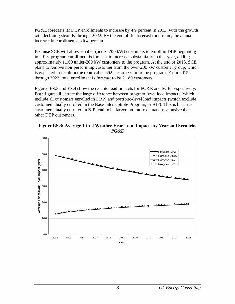
provided 122 kW of load impacts and AutoDR service accounts provided 16.8 MW. For SCE, TA/TI service accounts provided 6.4 MW of load impacts and AutoDR service accounts provided 13.2 MW. The baseline analysis analyzed measures of accuracy (how close the program baseline is to the "true" baseline) and bias (whether the program baseline has a tendency to be above or below the "true" baseline). The findings differed somewhat across utilities and customer groups. For PG&E, a 30 percent adjustment cap produces the most accurate baselines. For SCE, a 40 percent adjustment cap produces the most accurate baselines across all bidding customers, but a 20 percent cap is most accurate for customers who have selected the day-of adjustment. For PG&E, bias is slightly exacerbated by the day-of adjustment for customers who have selected it. However, the results show that the day-of adjustment (at any cap level) would nearly eliminate bias for the median customer among those who have not yet selected it. At SCE, the results indicate that bias is substantially reduced by the day-of adjustment, regardless of whether the customer has selected the day-of adjustment. For customers who have selected the optional adjustment, bias is minimized with a 20 percent adjustment cap. For customers who have not yet selected the optional adjustment, bias is minimized with a 40 percent cap. In the ex ante evaluation, SCE forecasts that DBP customer enrollment to increase substantially in 2013, decline slightly in 2014 and remain at that level through 2022. During this period, SCE's average event-hour load impact is approximately 89.9 MW. For PG&E, DBP enrollment increases by 4.9 percent in 2013 because of the incorporation of PeakChoice customers, after which the growth rate declines to approximately 0.4 percent by the end of the forecast timeframe. PG&E's program-level load impacts decline from 49.2 MW in 2012 to 34.0 MW in 2022. For both utilities, the portfolio-level load impacts are substantially less than the program-level load impacts because of the high level of load response provided by customers dually enrolled in the Base Interruptible Program (BIP). For SCE, the portfolio-level load impact is 11.9 MW from 2015-2022. For PG&E, the portfolio-level load impact increases from 12.8 MW in 2012 to 19.3 MW in 2022.
3 CA Energy Consulting
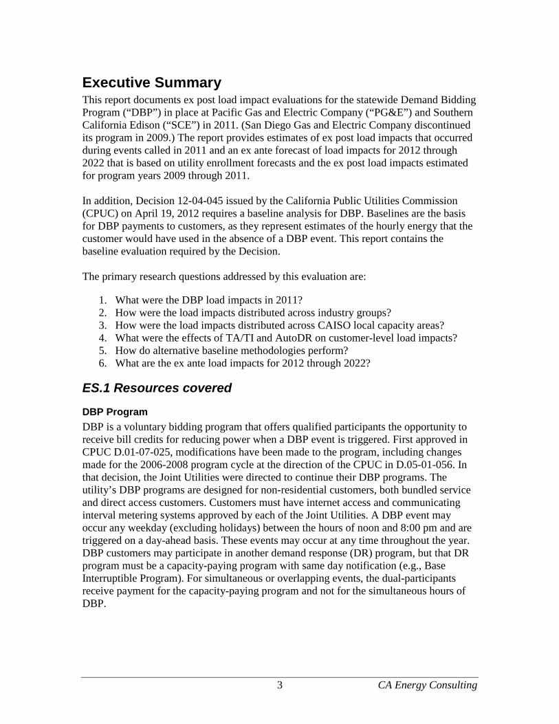
Executive Summary This report documents ex post load impact evaluations for the statewide Demand Bidding Program (“DBP”) in place at Pacific Gas and Electric Company (“PG&E”) and Southern California Edison (“SCE”) in 2011. (San Diego Gas and Electric Company discontinued its program in 2009.) The report provides estimates of ex post load impacts that occurred during events called in 2011 and an ex ante forecast of load impacts for 2012 through 2022 that is based on utility enrollment forecasts and the ex post load impacts estimated for program years 2009 through 2011. In addition, Decision 12-04-045 issued by the California Public Utilities Commission (CPUC) on April 19, 2012 requires a baseline analysis for DBP. Baselines are the basis for DBP payments to customers, as they represent estimates of the hourly energy that the customer would have used in the absence of a DBP event. This report contains the baseline evaluation required by the Decision. The primary research questions addressed by this evaluation are:
1. What were the DBP load impacts in 2011? 2. How were the load impacts distributed across industry groups? 3. How were the load impacts distributed across CAISO local capacity areas? 4. What were the effects of TA/TI and AutoDR on customer-level load impacts? 5. How do alternative baseline methodologies perform? 6. What are the ex ante load impacts for 2012 through 2022?
ES.1 Resources covered
DBP Program DBP is a voluntary bidding program that offers qualified participants the opportunity to receive bill credits for reducing power when a DBP event is triggered. First approved in CPUC D.01-07-025, modifications have been made to the program, including changes made for the 2006-2008 program cycle at the direction of the CPUC in D.05-01-056. In that decision, the Joint Utilities were directed to continue their DBP programs. The utility’s DBP programs are designed for non-residential customers, both bundled service and direct access customers. Customers must have internet access and communicating interval metering systems approved by each of the Joint Utilities. A DBP event may occur any weekday (excluding holidays) between the hours of noon and 8:00 pm and are triggered on a day-ahead basis. These events may occur at any time throughout the year. DBP customers may participate in another demand response (DR) program, but that DR program must be a capacity-paying program with same day notification (e.g., Base Interruptible Program). For simultaneous or overlapping events, the dual-participants receive payment for the capacity-paying program and not for the simultaneous hours of DBP.

4 CA Energy Consulting
PG&E called two test events in 2011, on September 8th and 22nd. The event window for both events was hours ending 15 through 18. SCE called five events, all of which were eight-hour events from hours-ending 13 through 20.
Enrollment Enrollment in PG&E’s DBP decreased slightly between the last two program years, from 1,052 in 2010 to 1,039 in 2011. The sum of enrolled customers’ non-coincident maximum demands amounted to 1,099 MW, or 1.1 MW per service account. Average hourly usage for enrolled customers was 725 MW, or 698 kW per service account. The manufacturing; and offices, hotels, health care and services industry groups made up the majority of PG&E’s DBP enrollment. Figure ES.1 illustrates the distribution of DBP load across the indicated industry types.
Figure ES.1 Distribution of DBP Enrollment by Industry Type – PG&E
Manufacturing39%
Whole., Trans., Util.14%
Retail3%
Offices, Hotels, Health, Services
26%
Schools2%
Other0%
Ent, Other svcs, Govt.10% Ag., Mining, Constr.
6%
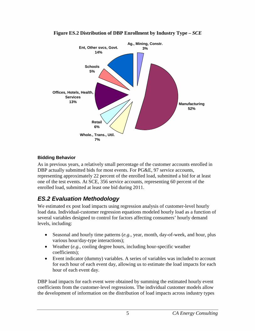
SCE’s enrollment in DBP decreased slightly from 1,421 service accounts in 2010 to 1,416 in 2011. These accounted for a total of 1,370 MW of maximum demand, or 1.0 MW per service account. Manufacturers continued to make up more than half of the enrolled load. Figure ES.2 illustrates the distribution of SCE’s DBP load across the indicated industry types.
5 CA Energy Consulting
Figure ES.2 Distribution of DBP Enrollment by Industry Type – SCE
Ag., Mining, Constr.3%
Manufacturing52%
Whole., Trans., Util.7%
Retail6%
Offices, Hotels, Health, Services
13%
Schools5%
Ent, Other svcs, Govt.14%
Bidding Behavior As in previous years, a relatively small percentage of the customer accounts enrolled in DBP actually submitted bids for most events. For PG&E, 97 service accounts, representing approximately 22 percent of the enrolled load, submitted a bid for at least one of the test events. At SCE, 356 service accounts, representing 60 percent of the enrolled load, submitted at least one bid during 2011.
ES.2 Evaluation Methodology We estimated ex post load impacts using regression analysis of customer-level hourly load data. Individual-customer regression equations modeled hourly load as a function of several variables designed to control for factors affecting consumers’ hourly demand levels, including:
• Seasonal and hourly time patterns (e.g., year, month, day-of-week, and hour, plus various hour/day-type interactions);
• Weather (e.g., cooling degree hours, including hour-specific weather coefficients);
• Event indicator (dummy) variables. A series of variables was included to account for each hour of each event day, allowing us to estimate the load impacts for each hour of each event day.
DBP load impacts for each event were obtained by summing the estimated hourly event coefficients from the customer-level regressions. The individual customer models allow the development of information on the distribution of load impacts across industry types

6 CA Energy Consulting
and geographical regions, by aggregating customer load impacts for the relevant industry group or local capacity area.
ES.3 Ex Post Load Impacts The total program load impact for PG&E’s test events averaged 57 MW, with a 67 MW load reduction (8.3 percent of enrolled load) for the first event, and 47 MW (5.6 percent of enrolled load) for the second event. Of the average 57 MW load impact across the two events, 45 MW came from customers enrolled in both DBP and BIP. For SCE, average hourly program load impacts averaged approximately 78 MW across four events.1 The load impacts across the four event days ranged from a low of 70 MW to a high of 89.5 MW. On average, the load impacts were approximately 7.6 percent of the total reference load. On a summary level, the average per-customer event-hour load impact was 55 kW for PG&E's program and 57 kW for SCE's program.
ES.4 TA/TI and AutoDR Effects We separately summarized average event-hour load impacts for customers participating in the Technical Assistance and Technology Incentives (TA/TI) program or the Automated Demand Response (AutoDR) program. Our goal was to estimate both total and incremental load impacts for TA/TI and AutoDR. Total load impacts are simply the sum of the estimated load impacts for the TA/TI and AutoDR customers, as estimated using the methods described in Section ES.2. Incremental load impacts are the load impacts achieved by these customers less the amount of the load impact one would expect in the absence of TA/TI or AutoDR. Given data limitations, we were unable to estimate reliable incremental load impacts. Specifically, we developed comparison groups according to industry classifications (SIC codes for SCE and NAICS codes for PG&E). Our findings revealed that the industry-level comparisons are based on too few customers to produce reliable results. In addition, we lack sufficient information on the comparison and "treatment" (AutoDR or TA/TI) customers to ensure that the comparison is valid. Specifically, we do not know relevant information about the comparison group customers, such as details regarding their technological processes (and hence their ability to reduce load during event hours) or whether they possess enabling technology. The total load estimated load impacts are summarized as follows. For PG&E, the TA/TI service account provided 122 kW of load impacts and AutoDR service accounts provided 16.8 MW. For SCE, TA/TI service accounts provided 6.4 MW of load impacts and AutoDR service accounts provided 13.2 MW.
1 A fifth event was called for October 13th, but this date fell outside of our analysis timeframe.
7 CA Energy Consulting
ES.5 Baseline Analysis DBP uses a 10-in-10 baseline method, including an optional day-of adjustment based on the ratio of the current day's pre-event usage level to the usage level in the same period for the 10-in-10 baseline.2 The tariff language currently limits this adjustment to +/- 20 percent. The utilities proposed an aggregated 10-in-10 baseline with the optional day-of adjustment limited to +/- 40%. As required by Decision 12-04-045, this report studies the following alternative baseline methodologies: unadjusted baselines, and day-of adjusted baselines with cap percentages of 20, 30, 40, and 50 percent, as well as an uncapped adjustment. Data from each event day from July 2011 through September 2011 were studied. The alternate baselines were compared to the estimated baseline load implied by the customer-specific regression models developed in the course of the DBP load impact evaluation. Measures of accuracy (how close the program baseline is to the "true" baseline) and bias (whether the program baseline has a tendency to be above or below the "true" baseline) were used in the evaluation. The findings differed somewhat across utilities and customer groups. For PG&E, a 30 percent adjustment cap produces the most accurate baselines. For SCE, a 40 percent adjustment cap produces the most accurate baselines across all bidding customers, though the error rate does not vary much with the cap level. However, removing the cap entirely produces a large reduction in baseline accuracy (this result is largely driven by the results for one large industrial customer). For customers who have selected the day-of adjustment, the variation in accuracy across alternative cap levels is larger, with a 20 percent cap level producing the most accurate baselines. For PG&E, bias is slightly exacerbated by the day-of adjustment for customers who have selected it, and the bias displays little variation across the alternative cap levels. However, the results show that the day-of adjustment (at any cap level) would nearly eliminate bias for the median customer among those who have not yet selected it. At SCE, the results indicate that bias is substantially reduced by the day-of adjustment. This is true regardless of whether the customer has selected the day-of adjustment. For customers who have selected the optional adjustment, bias is minimized with a 20 percent adjustment cap. For customers who have not yet selected the optional adjustment, bias is minimized with a 40 percent cap.
ES.6 Ex Ante Load Impacts Scenarios of ex ante load impacts are developed by combining enrollment forecasts with per-customer reference loads and load impacts, which were developed using the data and results of the ex post load impact evaluation.
2 The 10-in-10 baseline is calculated as the average energy usage for each hour across the ten most recent non-event weekdays. The day-of adjustment is calculated using average hourly consumption in the first three hours of the four hours prior to the event period.
8 CA Energy Consulting
PG&E forecasts its DBP enrollments to increase by 4.9 percent in 2013, with the growth rate declining steadily through 2022. By the end of the forecast timeframe, the annual increase in enrollments is 0.4 percent. Because SCE will allow smaller (under-200 kW) customers to enroll in DBP beginning in 2013, program enrollment is forecast to increase substantially in that year, adding approximately 1,100 under-200 kW customers to the program. At the end of 2013, SCE plans to remove non-performing customer from the over-200 kW customer group, which is expected to result in the removal of 662 customers from the program. From 2015 through 2022, total enrollment is forecast to be 2,189 customers. Figures ES.3 and ES.4 show the ex ante load impacts for PG&E and SCE, respectively. Both figures illustrate the large difference between program-level load impacts (which include all customers enrolled in DBP) and portfolio-level load impacts (which exclude customers dually enrolled in the Base Interruptible Program, or BIP). This is because customers dually enrolled in BIP tend to be larger and more demand responsive than other DBP customers.
Figure ES.3: Average 1-in-2 Weather Year Load Impacts by Year and Scenario, PG&E
0.0
10.0
20.0
30.0
40.0
50.0
60.0
2012 2013 2014 2015 2016 2017 2018 2019 2020 2021 2022
Year
Ave
rage
Eve
nt-H
our L
oad
Impa
ct (M
W)
Program 1in2Portfolio 1in10Portfolio 1in2Program 1in10

9 CA Energy Consulting
Figure ES.4: Average 1-in-2 Weather Year Load Impacts by Year and Scenario, SCE
0.0
10.0
20.0
30.0
40.0
50.0
60.0
70.0
80.0
90.0
100.0
2012 2013 2014 2015-2022
Year
Ave
rage
Eve
nt-H
our L
oad
Impa
ct (M
W)
Program 1in2Program 1in10Portfolio 1in2Portfolio 1in10

10 CA Energy Consulting
1. Introduction and Purpose of the Study This report documents ex post load impact evaluations for the statewide Demand Bidding Program (“DBP”) in place at Pacific Gas and Electric Company (“PG&E”) and Southern California Edison (“SCE”) in 2011. (San Diego Gas and Electric Company discontinued its program in 2009.) The report provides estimates of ex post load impacts that occurred during events called in 2011 and an ex ante forecast of load impacts for 2012 through 2022 that is based on utility enrollment forecasts and the ex post load impacts estimated for program years 2009 through 2011. In addition, Decision 12-04-045 issued by the California Public Utilities Commission (CPUC) on April 19, 2012 requires a baseline analysis for DBP. Baselines are the basis for DBP payments to customers, as they represent estimates of the hourly energy that the customer would have used in the absence of a DBP event. This report contains the baseline evaluation required by the Decision. The primary research questions addressed by this evaluation are:
1. What were the DBP load impacts in 2011? 2. How were the load impacts distributed across industry groups? 3. How were the load impacts distributed across CAISO local capacity areas? 4. What were the effects of TA/TI and AutoDR on customer-level load impacts? 5. How do alternative baseline methodologies perform? 6. What are the ex ante load impacts for 2012 through 2022?
The report is organized as follows. Section 2 contains a description of the DBP programs, the enrolled customers, and the events called; Section 3 describes the methods used in the study; Section 4 contains the detailed ex post load impact results, including estimates of the incremental effect of TA/TI and AutoDR on load impacts; Section 5 contains a study of the program baseline methodologies; Section 6 describes the ex ante load impact forecast; Section 7 contains an assessment of the validity of the study; and Section 8 provides recommendations.
2. Description of Resources Covered in the Study This section provides details on the Demand Bidding Programs, including the credits paid, the characteristics of the participants enrolled in the programs, and the events called in 2011.
2.1 Program Descriptions DBP is a voluntary bidding program that offers qualified participants the opportunity to receive bill credits for reducing power when a DBP event is triggered. First approved in CPUC D.01-07-025, modifications have been made to the program, including changes made for the 2006-2008 program cycle at the direction of the CPUC in D.05-01-056. In that decision, the Joint Utilities were directed to continue their DBP programs. The utility’s DBP programs are designed for non-residential customers, both bundled service and direct access customers. Customers must have internet access and communicating interval metering systems approved by each of the Joint Utilities. A DBP event may
11 CA Energy Consulting
occur any weekday (excluding holidays) between the hours of noon and 8:00 pm and are triggered on a day-ahead basis. These events may occur at any time throughout the year. DBP customers may participate in another demand response (DR) program, but that DR program must be a capacity-paying program with same day notification (e.g., Base Interruptible Program). For simultaneous or overlapping events, the dual-participants receive payment for the capacity-paying program and not for the simultaneous hours of DBP.
PG&E’s DBP Program At PG&E, DBP is available to time-of-use customers with billed maximum demands of 200 kW or higher (less for aggregated customer service accounts) who commit to reduce load by a minimum of 50 kW in each hour for two consecutive hours during a DBP event. Eligible customers must have an interval meter which is paid for by PG&E, except for direct access customers. For aggregated customer service accounts, there must be at least one service agreement with a maximum demand of 200 kW or greater for at least one or more of the past 12 billing months within each aggregated group that will be designated as the primary service agreement for the aggregated group. The DBP program operates year-round and can be called from 12:00 p.m. to 8:00 p.m. on weekdays, excluding holidays. There is no limit to the number of days on which DBP events may be called. Notification of an event day is provided on a day-ahead basis. Events are triggered with a California ISO Alert Notice for the following day when the California ISO’s day-ahead peak demand forecast is 43,000 MW or greater, or when PG&E, in its own opinion, forecasts that its other resources may not be sufficient or otherwise too costly to procure. PG&E may also activate up to two DBP test events per year in order to simulate an emergency event. When an event is called, enrolled customers may choose to bid a load reduction for the event or not to participate for that event. The incentive payment is $0.50 per kWh reduced below a baseline level. Customers must reduce load by a minimum of 50 percent of their bid amount to qualify for a credit, and they are paid for load reductions up to 150 percent of their bid amount. The hourly baseline for load reductions is calculated as the average usage from the previous ten qualifying days (non-holiday, non-event weekdays), with the customer having the option to include a day-of adjustment based on their usage in pre-event hours. There is no penalty for failing to comply with the terms of the submitted bid. Each bid must be a minimum of two consecutive hours during the event. Bids must meet the threshold of 50 kW for each hour and customers may submit only one bid for each event notification. Although PG&E customers enrolled in DBP may participate in other DR programs (Day-of notice in AMP, CBP, BIP, and OBMC), they do not receive a day-ahead DBP incentive payment for those hours in which a day-of event from another DR program in which the customer is enrolled occur simultaneously.

12 CA Energy Consulting
SCE’s DBP Program SCE’s DBP program design is similar to PG&E’s, with two exceptions: enrolled customers are required to commit to a minimum load reduction of 30 kW (versus 50 kW at PG&E); and bidding customers are paid for load reductions up to twice their bid amount. DBP participants may also participate in BIP or OBMC. However, the customer will not receive DBP incentive payments during overlapping event hours.
SDG&E’s DBP Program SDG&E discontinued its DBP in 2009.
2.2 Participant Characteristics
2.2.1 Development of Customer Groups In order to assess differences in load impacts across customer types, the program participants were categorized according to eight industry types. The industry groups are defined according to their applicable two-digit North American Industry Classification System (NAICS) codes:3
1. Agriculture, Mining and Oil and Gas, Construction: 11, 21, 23 2. Manufacturing: 31-33 3. Wholesale, Transport, other Utilities: 22, 42, 48-49 4. Retail stores: 44-45 5. Offices, Hotels, Finance, Services: 51-56, 62, 72 6. Schools: 61 7. Entertainment, Other services and Government: 71, 81, 92 8. Other or unknown.
In addition, each utility provided information regarding the CAISO Local Capacity Area (LCA) in which the customer resides (if any).4
2.2.2 Program Participants by Type The following sets of tables summarize the characteristics of the participating customer accounts, including size, industry type, and LCA. Table 2.1 shows DBP enrollment by industry group for PG&E. Enrollment in PG&E’s DBP decreased slightly between the last two program years, from 1,052 in 2010 to 1,039 in 2011.5 The sum of enrolled customers’ non-coincident maximum demands6, amounted to 1,099 MW, or 1.1 MW for 3 SCE provided Standard Industrial Classification (SIC) codes in place of NAICS codes. The industry groups were therefore defined according the following SIC codes: 1 = under 2000; 2 = 2000 to 3999; 3 = 4000 to 5199; 4 = 5200 to 5999; 5 = 6000 to 8199; 6 = 8200 to 8299; 7 = 8300 and higher. 4 Local Capacity Area (or LCA) refers to a CAISO-designated load pocket or transmission constrained geographic area for which a utility is required to meet a Local Resource Adequacy capacity requirement. There are currently seven LCAs within PG&E’s service area, 3 in SCE’s service territory, and 1 representing SDG&E’s entire service territory. In addition, PG&E has many accounts that are not located within any specific LCA. 5 "Enrollment" is defined as having been enrolled at any time during the program year. 6 Customer-level demand is calculated as the average of the monthly maximum demands during the program months.
13 CA Energy Consulting
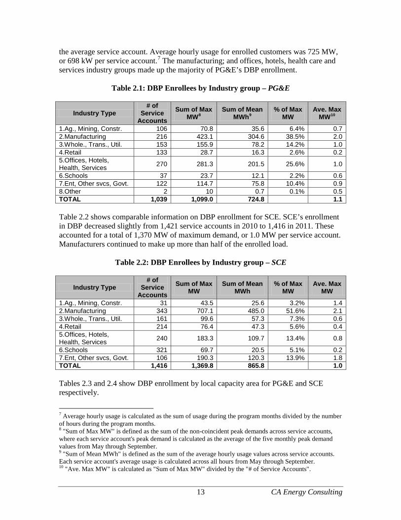
the average service account. Average hourly usage for enrolled customers was 725 MW, or 698 kW per service account.7 The manufacturing; and offices, hotels, health care and services industry groups made up the majority of PG&E’s DBP enrollment.
Table 2.1: DBP Enrollees by Industry group – PG&E
Industry Type # of
Service Accounts
Sum of Max MW8
Sum of Mean MWh9
% of Max MW
Ave. Max MW10
1.Ag., Mining, Constr. 106 70.8 35.6 6.4% 0.7 2.Manufacturing 216 423.1 304.6 38.5% 2.0 3.Whole., Trans., Util. 153 155.9 78.2 14.2% 1.0 4.Retail 133 28.7 16.3 2.6% 0.2 5.Offices, Hotels, Health, Services 270 281.3 201.5 25.6% 1.0
6.Schools 37 23.7 12.1 2.2% 0.6 7.Ent, Other svcs, Govt. 122 114.7 75.8 10.4% 0.9 8.Other 2 10 0.7 0.1% 0.5 TOTAL 1,039 1,099.0 724.8 1.1 Table 2.2 shows comparable information on DBP enrollment for SCE. SCE’s enrollment in DBP decreased slightly from 1,421 service accounts in 2010 to 1,416 in 2011. These accounted for a total of 1,370 MW of maximum demand, or 1.0 MW per service account. Manufacturers continued to make up more than half of the enrolled load.
Table 2.2: DBP Enrollees by Industry group – SCE
Industry Type # of
Service Accounts
Sum of Max MW
Sum of Mean MWh
% of Max MW
Ave. Max MW
1.Ag., Mining, Constr. 31 43.5 25.6 3.2% 1.4 2.Manufacturing 343 707.1 485.0 51.6% 2.1 3.Whole., Trans., Util. 161 99.6 57.3 7.3% 0.6 4.Retail 214 76.4 47.3 5.6% 0.4 5.Offices, Hotels, Health, Services 240 183.3 109.7 13.4% 0.8
6.Schools 321 69.7 20.5 5.1% 0.2 7.Ent, Other svcs, Govt. 106 190.3 120.3 13.9% 1.8 TOTAL 1,416 1,369.8 865.8 1.0 Tables 2.3 and 2.4 show DBP enrollment by local capacity area for PG&E and SCE respectively.
7 Average hourly usage is calculated as the sum of usage during the program months divided by the number of hours during the program months. 8 "Sum of Max MW" is defined as the sum of the non-coincident peak demands across service accounts, where each service account's peak demand is calculated as the average of the five monthly peak demand values from May through September. 9 "Sum of Mean MWh" is defined as the sum of the average hourly usage values across service accounts. Each service account's average usage is calculated across all hours from May through September. 10 "Ave. Max MW" is calculated as "Sum of Max MW" divided by the "# of Service Accounts".

14 CA Energy Consulting
Table 2.3: DBP Enrollees by Local Capacity Area – PG&E
Local Capacity Area
# of Service Accounts
Sum of Max MW
Sum of Mean MWh
% of Max MW
Ave. Max MW
Greater Bay Area 483 465.6 335.0 42.4% 1.0 Greater Fresno 55 46.7 29.8 4.2% 0.8 Humboldt 13 3.8 2.1 0.3% 0.3 Kern 53 38.0 22.0 3.5% 0.7 Northern Coast 74 45.8 25.7 4.2% 0.6 Not in any LCA 287 471.6 295.8 42.9% 1.6 Sierra 48 19.8 10.2 1.8% 0.4 Stockton 26 7.8 4.2 0.7% 0.3 TOTAL 1,039 1,099.0 724.8 1.1
Table 2.4: DBP Enrollees by Local Capacity Area – SCE Local Capacity
Area # of Service Accounts
Sum of Max MW
Sum of Mean MWh
% of Max MW
Ave. Max MW
LA Basin 1,110 906.1 562.5 66.1% 0.8 Outside LA Basin 67 184.2 120.5 13.4% 2.7 Ventura 239 279.5 182.8 20.4% 1.2 TOTAL 1,416 1,369.8 865.8 1.0 Tables 2.5 and 2.6 summarize the characteristics of customer accounts that submitted a bid for at least one 2011 event for PG&E and SCE respectively. For both utilities, the manufacturing industry group had the highest amount of load that submitted a bid.
Table 2.5: DBP Bidding Behavior – PG&E
Industry Type # Bidders
Sum of Max MW
% of Enrolled Max MW11
Avg. Hourly Bid MW
1.Ag., Mining, Constr. 4 9.6 13.6% 0.6 2.Manufacturing 24 127.4 30.1% 49.5 3.Whole., Trans., Util. 25 54.6 35.0% 13.6 4.Retail 15 10.7 37.3% 3.1 5.Offices, Hotels, Health, Services 16 52.2 18.6% 1.9
6.Schools 2 2.9 12.2% 0.3 7. Ent, Other svcs, Govt. 11 48.9 42.6% 3.6 TOTAL 97 306.3 27.9% 72.6
11 "% of Enrolled Max kW" is defined as the "Sum of Max kW" for bidders divided by the corresponding value for all enrolled customers, where the calculation is performed by industry group.

15 CA Energy Consulting
Table 2.6: DBP Bidding Behavior – SCE
Industry Type # Bidders
Sum of Max MW
% of Enrolled Max MW
Avg. Hourly Bid MW
1.Ag., Mining, Constr. 14 24.3 55.9% 7.1 2.Manufacturing 139 450.3 63.7% 113.5 3.Whole., Trans., Util. 52 67.7 68.0% 10.6 4.Retail 24 43.7 57.2% 4.0 5.Offices, Hotels, Health, Services 84 97.3 53.1% 7.5
6.Schools 23 30.5 43.8% 1.7 7. Ent, Other svcs, Govt. 20 107.6 56.5% 2.5 TOTAL 356 821.4 60.0% 146.9
2.3 Event Days Table 2.7 lists DBP event days for the two utilities in 2011. PG&E called two test events, on September 8th and 22nd. The event window for both events was hours ending 15 through 18. SCE called five events, all of which were eight-hour events from hours-ending 13 through 20.
Table 2.7: DBP Events – 2011 Date Day of Week SCE PG&E
7/5/2011 Tuesday 1 8/26/2011 Friday 2
9/7/2011 Wednesday 3 9/8/2011 Thursday 4 1 (Test)
9/22/2011 Thursday 2 (Test) 10/13/2011 Thursday 5
3. Study Methodology
3.1 Overview We estimated ex post hourly load impacts using regression equations applied to customer-level hourly load data. The regression equation models hourly load as a function of a set of variables designed to control for factors affecting consumers’ hourly demand levels, such as:
• Seasonal and hourly time patterns (e.g., year, month, day-of-week, and hour, plus various hour/day-type interactions);
• Weather (e.g., cooling degree hours, including hour-specific weather coefficients);
• Event variables. A series of dummy variables was included to account for each hour of each event day, allowing us to estimate the load impacts for all hours across the event days.
16 CA Energy Consulting
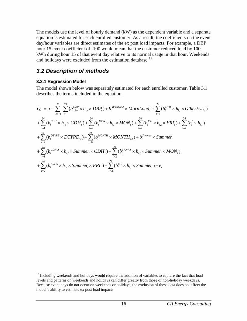
The models use the level of hourly demand (kW) as the dependent variable and a separate equation is estimated for each enrolled customer. As a result, the coefficients on the event day/hour variables are direct estimates of the ex post load impacts. For example, a DBP hour 15 event coefficient of -100 would mean that the customer reduced load by 100 kWh during hour 15 of that event day relative to its normal usage in that hour. Weekends and holidays were excluded from the estimation database.12
3.2 Description of methods
3.2.1 Regression Model The model shown below was separately estimated for each enrolled customer. Table 3.1 describes the terms included in the equation.
ti
ttiSh
ii
tttiSFRI
i
ittti
SMONi
ittti
SCDHi
tSummert
iti
MONTHi
iti
DTYPEi
iti
hi
itti
FRIi
itti
MONi
itti
CDHi
i ititi
OTHit
MornLoadtti
DBPEvti
E
Evtt
eSummerhbFRISummerhb
MONSummerhbCDHSummerhb
SummerbMONTHbDTYPEb
hbFRIhbMONhbCDHhb
OtherEvthbMornLoadbDBPhbaQ
+××+×××+
×××+×××+
×+×+×+
×+××+××+××+
××+×+××+=
∑∑
∑∑
∑∑
∑∑∑∑
∑ ∑∑
==
==
==
====
= ==
)()(
)()(
)()(
)()()()(
)()(
24
2,
,24
2,
,
24
2,
,24
1,
,
10
6,
5
2,
24
2,
24
2,
24
2,
24
1,
24
1
24
1,,,,
1
12 Including weekends and holidays would require the addition of variables to capture the fact that load levels and patterns on weekends and holidays can differ greatly from those of non-holiday weekdays. Because event days do not occur on weekends or holidays, the exclusion of these data does not affect the model’s ability to estimate ex post load impacts.

17 CA Energy Consulting
Table 3.1: Descriptions of Terms included in the Ex Post Regression Equation Variable Name
/ Term Variable / Term Description
Qt the demand in hour t for a customer enrolled in DBP prior to the last event date
The various b’s the estimated parameters hi,t a dummy variable for hour i
DBPt an indicator variable for program event days CDHt cooling degree hours13
E the number of event days that occurred during the program year MornLoadt a variable equal to the average of the day’s load in hours 1 through 10
OtherEvtt equals one in the event hours of other demand response programs in which the customer is enrolled
MONt a dummy variable for Monday FRIt a dummy variable for Friday
DTYPEi,t a series of dummy variables for each day of the week MONTHi,t a series of dummy variables for each month
Summert a variable indicating summer months (defined as mid-June through mid-August)14, which is interacted with the weather and hourly profile variables
et the error term. The “morning load” variable was used in lieu of a more formal autoregressive structure in order to adjust the model to account for the level of load on a particular day. Because of the autoregressive nature of the morning load variable, no further correction for serial correlation was performed in these models. Separate models were estimated for each customer. The load impacts were aggregated across customer accounts as appropriate to arrive at program-level load impacts, as well as load impacts by industry group and local capacity area (LCA).
3.2.2 Development of Uncertainty-Adjusted Load Impacts The Load Impact Protocols require the estimation of uncertainty-adjusted load impacts. In the case of ex post load impacts, the parameters that constitute the load impact estimates are not estimated with certainty. We base the uncertainty-adjusted load impacts on the variances associated with the estimated load impact coefficients. Specifically, we added the variances of the estimated load impacts across the customers who submit a bid for the event in question. These aggregations were performed at either the program level, by industry group, or by LCA, as appropriate. The uncertainty-adjusted scenarios were then simulated under the assumption that each hour’s load impact is normally distributed with the mean equal to the sum of the estimated load impacts and the standard deviation equal to the square root of the sum of the variances of the errors 13 Cooling degree hours (CDH) was defined as MAX[0, Temperature – 50], where Temperature is the hourly temperature in degrees Fahrenheit. Customer-specific CDH values are calculated using data from the most appropriate weather station. 14 This variable was initially designed to reflect the load changes that occur when schools are out of session. We have found the variables to a useful part of the base specification, as they reflect changes in usage patterns and weather response that differ during the analysis timeframe for many customers, even those that are not schools.

18 CA Energy Consulting
around the estimates of the load impacts. Results for the 10th, 30th, 70th, and 90th percentile scenarios are generated from these distributions.
4. Detailed Study Findings The primary objective of the ex post evaluation is to estimate the aggregate and per-customer DBP event-day load impacts for each utility. In this section we first summarize the estimated DBP load impacts for both utilities’ using a metric of estimated average hourly load impacts by event and for the average event. We also report average hourly load impacts for the average event by industry type and local capacity area. We then present tables of hourly load impacts for an average event (also referred to as a “typical event day”) in the format required by the Load Impact Protocols adopted by the California Public Utilities Commission (CPUC) in Decision (D.) 08-04-050 (“the Protocols”), including risk-adjusted load impacts at different probability levels, and figures that illustrate the reference loads, observed loads and estimated load impacts. The section concludes with an assessment of the effects of TA/TI and AutoDR. On a summary level, the average event-hour load impact per enrolled customer was 55 kW for PG&E's program and 53 kW for SCE's program.
4.1 PG&E Load Impacts
4.1.1 Average Hourly Load Impacts by Industry Group and LCA Table 4.1 summarizes average hourly reference loads and load impacts at the program level for each of PG&E’s two DBP events. The average hourly load impact across both events was 57 MW. The average load impact on the first event day was 20 MW higher than the load impact on the second event day. On average, the load impacts were 7.0 percent of the total reference load.
Table 4.1: 2011 Average Hourly Load Impacts by Event, PG&E
Event Date Day of Week
Estimated Reference Load
(MW) Observed Load (MW)
Estimated Load Impact (MW) % LI
1 9/8/2011 Thursday 810 742 67 8.3% 2 9/22/2011 Thursday 825 779 47 5.6%
Average 818 761 57 7.0% Std. Dev. 11 26 15 1.8%
Table 4.2 compares the bid quantities to the estimated load impacts for each event. Across both events, the bid amount averaged approximately 57.6 MW, while the estimated average hourly load impact was 56.9 MW. The average bid realization rate (estimated load impacts as a percentage of bid amounts) across all event hours was 99 percent.

19 CA Energy Consulting
Table 4.2: 2011 Average Hourly Bid Realization Rates by Event, PG&E
Event Date Day of Week
Average Bid Quantity (MW)
Estimated Load Impact (MW)
LI as % of Bid Amount
1 9/8/2011 Thursday 64.7 67.2 104% 2 9/22/2011 Thursday 50.5 46.5 92%
Average 57.6 56.9 99% Table 4.3 summarizes average hourly DBP load impacts at the program level (i.e., including both bidders and non-bidders) and by industry group for each of PG&E’s event days. Across all event hours, the average hourly load impact was 57 MW, or 7.0 percent of enrolled load. The Manufacturing industry group accounted for the largest share of the load impacts.
Table 4.3: 2011 Average Hourly Load Impacts – PG&E DBP, by Industry Group
Industry Group # of Service Accounts
Estimated Reference Load (MW)
Observed Load (MW)
Estimated Load Impact
(MW) % LI
Agriculture, Mining, & Construction 105.5 36.9 35.9 1.0 2.7%
Manufacturing 216 326.6 294.8 31.8 9.7% Wholesale, Transportation, & Other Utilities
153 73.2 55.2 18.0 24.6%
Retail Stores 133 22.8 20.9 1.9 8.5% Offices, Hotels, Health, Services 270 246.2 245.4 0.8 0.3%
Schools 37 18.8 19.4 -0.5 -2.7% Entertainment, Other Services, Government
122 92.2 88.5 3.7 4.0%
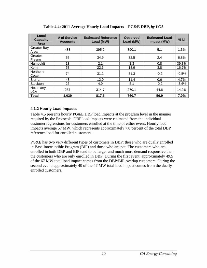
Other or Unknown 2 0.8 0.7 0.1 8.6% Total 1,039 817.6 760.7 56.9 7.0% Table 4.4 summarizes load impacts by local capacity area (LCA), showing that the highest share of the load impacts came from service accounts not associated with any LCA.
20 CA Energy Consulting
Table 4.4: 2011 Average Hourly Load Impacts – PG&E DBP, by LCA
Local Capacity
Area # of Service Accounts
Estimated Reference Load (MW)
Observed Load (MW)
Estimated Load Impact (MW) % LI
Greater Bay Area 483 395.2 390.1 5.1 1.3%
Greater Fresno 55 34.9 32.5 2.4 6.8%
Humboldt 13 2.1 1.3 0.8 39.3% Kern 53 22.6 18.9 3.8 16.7% Northern Coast 74 31.2 31.3 -0.2 -0.5%
Sierra 48 12.0 11.4 0.6 4.7% Stockton 26 4.9 5.1 -0.2 -3.6% Not in any LCA 287 314.7 270.1 44.6 14.2%
Total 1,039 817.6 760.7 56.9 7.0%
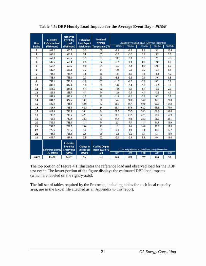
4.1.2 Hourly Load Impacts Table 4.5 presents hourly PG&E DBP load impacts at the program level in the manner required by the Protocols. DBP load impacts were estimated from the individual customer regressions for customers enrolled at the time of either event. Hourly load impacts average 57 MW, which represents approximately 7.0 percent of the total DBP reference load for enrolled customers. PG&E has two very different types of customers in DBP: those who are dually enrolled in Base Interruptible Program (BIP) and those who are not. The customers who are enrolled in both DBP and BIP tend to be larger and much more demand responsive than the customers who are only enrolled in DBP. During the first event, approximately 49.5 of the 67 MW total load impact comes from the DBP/BIP-overlap customers. During the second event, approximately 40 of the 47 MW total load impact comes from the dually enrolled customers.
21 CA Energy Consulting
Table 4.5: DBP Hourly Load Impacts for the Average Event Day – PG&E
Uncertainty Adjusted Impact (MWh/ hr)- Percentiles10th%ile 30th%ile 50th%ile 70th%ile 90th%ile
1 667.2 665.7 1.5 66 -7.3 -2.1 1.5 5.2 10.42 659.1 658.9 0.1 65 -8.7 -3.5 0.1 3.7 9.03 652.0 653.5 -1.5 63 -10.3 -5.1 -1.5 2.1 7.34 649.6 650.4 -0.8 62 -9.7 -4.4 -0.8 2.8 8.05 658.7 659.6 -0.8 61 -9.6 -4.4 -0.8 2.8 8.06 689.7 693.4 -3.7 61 -12.5 -7.3 -3.7 -0.1 5.17 734.1 738.7 -4.6 60 -13.4 -8.2 -4.6 -1.0 4.28 758.0 758.0 0.0 60 -8.8 -3.6 0.0 3.6 8.89 783.1 786.0 -2.9 63 -11.7 -6.5 -2.9 0.7 5.910 802.1 807.9 -5.8 66 -14.6 -9.4 -5.8 -2.2 3.011 818.6 824.8 -6.1 70 -14.9 -9.7 -6.1 -2.5 2.712 829.6 833.7 -4.1 74 -12.9 -7.7 -4.1 -0.5 4.713 832.6 835.5 -2.9 77 -11.8 -6.5 -2.9 0.7 5.914 841.7 827.5 14.2 80 5.4 10.6 14.2 17.8 23.015 840.4 781.4 59.0 82 50.2 55.4 59.0 62.6 67.816 825.6 763.4 62.2 84 53.4 58.6 62.2 65.8 71.017 817.5 758.4 59.1 84 50.3 55.5 59.1 62.8 68.018 786.7 739.6 47.1 82 38.3 43.5 47.1 50.7 55.919 762.4 739.2 23.3 79 14.4 19.6 23.3 26.9 32.120 749.5 738.4 11.1 74 2.3 7.5 11.1 14.7 19.921 739.7 729.7 10.0 71 1.2 6.4 10.0 13.6 18.822 725.5 718.6 6.9 69 -2.0 3.3 6.9 10.5 15.723 704.3 701.2 3.1 68 -5.8 -0.6 3.1 6.7 11.924 689.7 687.0 2.8 67 -6.1 -0.9 2.8 6.4 11.6
Uncertainty Adjusted Impact (MWh/ hour) - Percentiles10th 30th 50th 70th 90th
Daily 18,018 17,751 267 33.9 n/a n/a n/a n/a n/a
Weighted Average
Temperature (oF)
Reference Energy Use (MWh)
Estimated Event Day
Energy Use (MWh)
Change in Energy Use
(MWh)
Cooling Degree Hours (Base 75
oF)
Hour Ending
Estimated Reference Load
(MWh/hour)
Observed Event Day
Load (MWh/hour)
Estimated Load Impact (MWh/hour)
The top portion of Figure 4.1 illustrates the reference load and observed load for the DBP test event. The lower portion of the figure displays the estimated DBP load impacts (which are labeled on the right y-axis). The full set of tables required by the Protocols, including tables for each local capacity area, are in the Excel file attached as an Appendix to this report.

22 CA Energy Consulting
Figure 4.1: 2011 DBP Load Impacts – PG&E
0
100
200
300
400
500
600
700
800
900
1 2 3 4 5 6 7 8 9 10 11 12 13 14 15 16 17 18 19 20 21 22 23 24
Hour
Load
(MW
)
-10
0
10
20
30
40
50
60
70
80
Load
Impa
ct (M
W)
ReferenceObservedLoad Impact
4.2 SCE Load Impacts
4.2.1 Average Hourly Load Impacts by Industry Group and LCA Table 4.6 summarizes average hourly reference loads and load impacts at the program level for each of SCE’s four DBP events.15 Across all events, the average hourly load impact was approximately 78 MW. The load impacts showed little variation across event days, with a low of 70 MW, a high of 89.5 MW, and a standard deviation of 8 MW. On average, the load impacts were 7.6 percent of the total reference load.
Table 4.6: 2011 Average Hourly Load Impacts by Event, SCE
Event Date Day of Week
Estimated Reference Load
(MW) Observed Load (MW)
Estimated Load Impact (MW) % LI
1 7/5/2011 Tuesday 939.0 865.0 74.0 7.9% 2 8/26/2011 Friday 1,036.0 965.7 70.3 6.8% 3 9/7/2011 Wednesday 1,069.0 992.3 76.8 7.2% 4 9/8/2011 Thursday 1,051.5 962.0 89.5 8.5%
Average 1,023.9 946.2 77.7 7.6% Std. Dev. 58.2 55.8 8.3 0.8%
15 A fifth event day was called on October 13, 2011, but this date falls outside of our analysis timeframe, which ends on September 30, 2011.

23 CA Energy Consulting
Table 4.7 compares the bid quantities to the estimated load impacts for each event. Across all events, the bid amount averaged approximately 129.1 MW, while the estimated average hourly load impact was 77.7 MW. The average bid realization rate (estimated load impacts as a percentage of bid amounts) across all event hours was 60 percent.
Table 4.7: 2011 Average Hourly Bid Realization Rates by Event, SCE
Event Date Day of Week
Average Bid Quantity (MW)
Estimated Load Impact (MW)
LI as % of Bid Amount
1 7/5/2011 Tuesday 134.2 74.0 55% 2 8/26/2011 Friday 111.7 70.3 63% 3 9/7/2011 Wednesday 132.1 76.8 58% 4 9/8/2011 Thursday 138.5 89.5 65%
Average 129.1 77.7 60% Tables 4.8 and 4.9 summarize average hourly load impacts for the average event by industry group and LCA. Manufacturing service accounts accounted for the largest share of the load impacts. By region, the highest share of the average load impact came from the LA Basin.
Table 4.8: 2011 Average Hourly Load Impacts – SCE DBP, by Industry Group
Industry Group # of Service Accounts
Estimated Reference Load (MW)
Observed Load (MW)
Estimated Load Impact
(MW) % LI
Agriculture, Mining, & Construction 29 27.2 24.4 2.9 10.5%
Manufacturing 333 532.9 472.1 60.8 11.4% Wholesale, Transportation, & Other Utilities
155 59.5 51.5 8.0 13.5%
Retail Stores 202 60.1 58.1 2.0 3.4% Offices, Hotels, Health, Services 231 145.5 144.4 1.1 0.7%
Schools 300 39.5 38.1 1.4 3.4% Entertainment, Other Services, Government
104 159.2 157.7 1.5 1.0%
Total 1,354 1,023.9 946.2 77.7 7.6%
Table 4.9: 2011 Average Hourly Load Impacts – SCE DBP, by LCA
Local Capacity Area
# of Service
Accounts
Estimated Reference Load
(MW) Observed Load (MW)
Estimated Load Impact
(MW) % LI
LA Basin 1,059 673.0 620.5 52.5 7.8% Outside LA Basin
64 137.3 122.9 14.4 10.5%
Ventura 230 213.5 202.8 10.7 5.0% Total 1,354 1,023.9 946.2 77.7 7.6%

24 CA Energy Consulting
4.2.2 Hourly Load Impacts Table 4.10 presents hourly load impacts at the program level for the average DBP event in the manner required by the Protocols. Hourly load impacts for the average event range from 65 MW to 84 MW. These load impacts represent 7.6 percent of the total enrolled DBP reference load.
Table 4.10: 2011 DBP Hourly Load Impacts for the Average Event Day, SCE
Uncertainty Adjusted Impact (MWh/ hr)- Percentiles10th%ile 30th%ile 50th%ile 70th%ile 90th%ile
1 812.2 794.0 18.2 76 4.9 12.7 18.2 23.6 31.52 800.7 785.1 15.6 75 2.3 10.2 15.6 21.1 29.03 789.9 776.0 13.9 74 0.5 8.4 13.9 19.3 27.24 790.5 778.6 11.9 73 -1.4 6.4 11.9 17.4 25.35 810.0 800.0 10.0 72 -3.3 4.6 10.0 15.5 23.46 855.4 846.3 9.1 71 -4.3 3.6 9.1 14.6 22.57 905.2 900.1 5.1 70 -8.2 -0.3 5.1 10.6 18.58 951.6 957.0 -5.4 70 -18.7 -10.9 -5.4 0.1 8.09 999.9 1,013.9 -14.0 72 -27.4 -19.5 -14.0 -8.6 -0.710 1,034.0 1,042.4 -8.4 76 -21.8 -13.9 -8.4 -3.0 4.911 1,065.6 1,066.1 -0.5 80 -13.8 -5.9 -0.5 5.0 12.912 1,079.4 1,047.7 31.6 83 18.3 26.2 31.6 37.1 45.013 1,078.2 1,004.2 74.0 86 60.7 68.6 74.0 79.5 87.314 1,083.3 1,006.5 76.8 88 63.5 71.4 76.8 82.3 90.115 1,078.0 998.3 79.7 89 66.4 74.3 79.7 85.1 93.016 1,052.8 971.8 81.0 90 67.6 75.5 81.0 86.4 94.317 1,023.3 941.0 82.4 89 69.1 77.0 82.4 87.8 95.718 991.1 907.5 83.6 89 70.3 78.2 83.6 89.0 96.919 951.2 872.7 78.5 88 65.2 73.0 78.5 83.9 91.820 933.3 868.0 65.2 85 51.9 59.8 65.2 70.7 78.621 918.2 874.9 43.3 82 30.0 37.9 43.3 48.8 56.722 891.1 865.1 25.9 79 12.6 20.5 25.9 31.4 39.223 856.4 829.8 26.5 77 13.2 21.1 26.5 32.0 39.824 833.5 813.8 19.7 76 6.3 14.2 19.7 25.1 33.0
Uncertainty Adjusted Impact (MWh/ hour) - Percentiles10th 30th 50th 70th 90th
Daily 22,585 21,761 824 132.2 n/a n/a n/a n/a n/a
Weighted Average
Temperature (oF)
Reference Energy Use (MWh)
Estimated Event Day
Energy Use (MWh)
Change in Energy Use
(MWh)
Cooling Degree Hours (Base 75
oF)
Hour Ending
Estimated Reference Load
(MWh/hour)
Observed Event Day
Load (MWh/hour)
Estimated Load Impact (MWh/hour)
The top portion of Figure 4.2 illustrates the hourly reference load and observed load for the average DBP event. The bottom portion of Figure 4.2 displays the estimated hourly load impacts (scale is presented on the right y-axis) for the average DBP event. Figure 4.3 shows the variability of estimated load impacts across events. The load impacts were quite consistent across events, particularly when compared to SCE's load impacts from the previous program year.

25 CA Energy Consulting
Figure 4.2: 2011 DBP Load Impacts – SCE
0
200
400
600
800
1,000
1,200
1 2 3 4 5 6 7 8 9 10 11 12 13 14 15 16 17 18 19 20 21 22 23 24
Hour
Load
(MW
)
-20
0
20
40
60
80
100
Load
Impa
ct (M
W)
ReferenceObservedLoad Impact
Figure 4.3: 2011 Hourly Load Impacts by Event – SCE DBP
-40.0
-20.0
0.0
20.0
40.0
60.0
80.0
100.0
120.0
1 2 3 4 5 6 7 8 9 10 11 12 13 14 15 16 17 18 19 20 21 22 23 24
Hour
Load
Impa
ct (M
W)
Average Event Day7/5/20118/26/20119/7/20119/8/2011
4.3 Effect of TA/TI and AutoDR on Load Impacts This section describes the ex post load impacts achieved by DBP customer accounts that participated in two demand response incentive programs: TA/TI and AutoDR.

26 CA Energy Consulting
The Technical Assistance and Technology Incentives (TA/TI) program has two parts: technical assistance in the form of energy audits, and technology incentives. The objective of the TA portion of the program is to subsidize customer energy audits that have the objective of identifying ways in which customers can reduce load during demand response events. The TI portion of the program then provides incentive payments for the installation of equipment or control software supporting DR. The Automated Demand Response (AutoDR) program helps customers to activate DR strategies, such as managing lighting or heating, ventilation and air conditioning (HVAC) systems, whereby electrical usage can be automatically reduced or eliminated during times of high electricity prices or electricity system emergencies. Our goal was to estimate both total and incremental load impacts for TA/TI and AutoDR. Total load impacts are simply the sum of the estimated load impacts for the TA/TI and AutoDR customers, as estimated using the methods described in Section 3.2.1. Incremental load impacts are the load impacts achieved by these customers less the amount of the load impact one would expect in the absence of TA/TI or AutoDR. Given data limitations, we were unable to estimate reliable incremental load impacts. Specifically, we developed comparison groups according to industry classifications (SIC codes for SCE and NAICS codes for PG&E). Where possible, we compared customers within a 6-digit NAICS code or 4-digit SIC code. Where a comparison at this level of disaggregation was not possible, we compared at a higher level of industry aggregation, such as using one of the eight industry groups described in Section 2.2.1. Our findings revealed that the industry-level comparisons are based on too few customers to produce reliable results. We considered aggregating AutoDR and TA/TI customers into larger industry groups as a solution to the sample-size issue, but this solution raises serious questions about the comparability of the results between the two groups. We have found that percentage load impacts can vary substantially across industry sub-groups, which calls into question the reasonableness of comparing customers within a higher-level industry group (e.g., all manufacturing customers). In addition, we lack sufficient information on the comparison and "treatment" (AutoDR or TA/TI) customers to ensure that the comparison is valid. Specifically, we do not know relevant information about the comparison group customers, such as details regarding their technological processes (and hence their ability to reduce load during event hours) or whether they possess enabling technology. For each utility and incentive program, we present two tables. The first table (e.g., Table 4.11) contains the overall average hourly load impacts provided by the service accounts that participated in TA/TI or AutoDR. The second table (e.g., Table 4.12) displays the number of service accounts by industry group for the comparison group customers and the AutoDR or TA/TI customers. This table format illustrates the small sample size issue described above.

27 CA Energy Consulting
The sub-sections below present the results for each of the utilities.
PG&E TA/TI According to data provided by PG&E, one DBP service account participating in the TA/TI program submitted a bid for the September 8, 2011 event. No such service accounts submitted a bid for the September 22, 2011 event. Table 4.11 shows the event-specific load impact for the TA/TI participant. The TA/TI customer provided an average hourly load reduction of 122 kW, or 3.1 percent of their reference load.
Table 4.11: Average Hourly Load Impacts by Event, PG&E TA/TI Event Date
Number of SAIDs
Estimated Reference Load (kW)
Observed Load (kW)
Estimated Load Impact (kW)
% Load Impact
9/8/2011 1 4,062 3,940 122 3.1% As shown in Table 4.12, only one service account is present in the comparison and treatment groups, raising questions about the reasonableness of a comparison of the responsiveness between them.
Table 4.12: Number of Service Accounts by Group , PG&E TA/TI
NAICS Code NAICS Description Basis of Comparison
Number of SAIDs
No TA/TI TA/TI 541380 Testing Laboratories 6-digit NAICS 1 1
AutoDR According to data provided by PG&E, an average of 65 DBP service accounts participating in the AutoDR program submitted a bid for the 2011 test events. Table 4.13 shows the average hourly load impact for the AutoDR participants, which was 16,835 kW, or 30 percent of their reference load. Note that the total and percentage load impacts are strongly influenced by one SAID that reduced its load by 100 percent, or 13.8 MW.
Table 4.13: Average Hourly Load Impacts by Event, PG&E AutoDR Event Date
Number of SAIDs
Estimated Reference Load (kW)
Observed Load (kW)
Estimated Load Impact (kW)
% Load Impact
9/8/11 67 50,772 35,720 15,052 29.6% 9/22/11 62 61,341 42,722 18,618 30.4% Average 65 56,057 39,221 16,835 30.0% AutoDR participants were spread across 25 6-digit NAICS industry codes. In nine of these industry groups, non-AutoDR bidders are present to serve as a comparison group. For the remaining 16 industry groups with Auto-DR customers, comparisons are made at a more aggregated level. The “Basis of Comparison” column identifies the industry level used for the comparison group. Table 4.14 shows the sample size by industry group.

28 CA Energy Consulting
Twenty-two of the twenty-five industry groups contain a comparison in which at least one of the groups has only one service account.
Table 4.14: Number of Service Accounts by Group, PG&E AutoDR
NAICS Code NAICS Description
Basis of Comparison
Number of SAIDs No
AutoDR AutoDR 115114 Postharvest Crop Activities (except Cotton Ginning) 6-Digit 1 3
221112 Fossil Fuel Electric Power Generation Utilities, Wholesale 17 1
325120 Industrial Gas Manufacturing Manufacturing 14 1
334112 Computer Storage Device Manufacturing 6-Digit 1 6
423930 Recyclable Material Merchant Wholesalers Utilities, Wholesale 17 1
424410 General Line Grocery Merchant Wholesalers Utilities, Wholesale 17 1
452111 Department Stores (except Discount Department Stores) 6-Digit 1 23
518210 Data Processing, Hosting, and Related Services 6-Digit 2 2
53112 Lessors of Nonresidential Buildings (except Miniwarehouses) 5-Digit 2 1
54171 Research and Development in the Physical, Engineering, and Life Sciences 5-Digit 1 2
551114 Corporate, Subsidiary, and Regional Managing Offices 6-Digit 1 2
6214 Outpatient Care Centers Information 12 1
621491 HMO Medical Centers Information 12 1
62211 General Medical and Surgical Hospitals Information 12 1
624 Social Assistance Information 12 1
624190 Other Individual and Family Services Information 12 1
624310 Vocational Rehabilitation Services Information 12 1
713940 Fitness and Recreational Sports Centers 6-Digit 10 4
812910 Pet Care (except Veterinary) Services Arts, Entertainment 18 1
921190 Other General Government Support 6-Digit 2 7
922120 Police Protection 2-Digit 6 1
922130 Legal Counsel and Prosecution 2-Digit 6 1
922140 Correctional Institutions 6-Digit 1 3
922160 Fire Protection 2-Digit 6 1
923130 Administration of Human Resource Programs (except Education, Public Health, and Veterans' Affairs Programs) 6-Digit 1 1

29 CA Energy Consulting
SCE TA/TI Table 4.15 shows the DBP load impacts provided by SCE’s TA/TI service accounts for each event. An average of 51 of SCE’s DBP service accounts participated in TA/TI. The load impacts are much higher for the first event than the subsequent events. This is due to one service account that provided essentially no load impact for three events, but provided approximately 19 MW of load response for the first event. The load impacts in the absence of this customer average 1.7 MW, or 4.8 percent of the remaining reference load.
Table 4.15: Average Hourly TA/TI Load Impacts by Event, SCE TA/TI
Event Date
Number of SAIDs
Estimated Reference Load (kW)
Observed Load (kW)
Estimated Load Impact (kW)
% Load Impact
7/5/11 51 52,222 31,032 21,190 40.6%
8/26/11 51 55,108 53,248 1,859 3.4%
9/7/11 51 54,457 53,136 1,322 2.4%
9/8/11 51 54,328 53,253 1,074 2.0% Average 51 54,029 47,667 6,361 11.8%
Table 4.16 shows the number of service accounts by industry group. Eight of the fourteen industry groups contain a comparison in which at least one of the groups has only one service account.

30 CA Energy Consulting
Table 4.16: Number of Service Accounts by Group, SCE TA/TI
SIC Code SIC Description
Basis of Comparison
Number of SAIDs
No TA/TI TA/TI
2026 Fluid Milk 2 Dig. SIC 2 1
2041 Flour and Other Grain Mill Products 4 Dig. SIC 2 1
2813 Industrial Gases 4 Dig. SIC 4 2
2834 Pharmaceutical Preparations 4 Dig. SIC 2 1
3728 Aircraft Parts and Equipment, NEC 4 Dig. SIC 2 1
5072 Hardware 1 Dig. SIC 11 2
5318 Shopping Centers-Retail Sales 4 Dig. SIC 1 1
5411 Grocery Stores 4 Dig. SIC 8 13 5651 Family Clothing Stores 4 Dig. SIC 1 2
5912 Drug Stores and Proprietary Stores 1 Dig. SIC 11 1
6512 Nonresidential Building Operators 4 Dig. SIC 18 21
6514 Dwelling Operators, Exc. Apartments 4 Dig. SIC 6 4
7011 Hotels and Motels 4 Dig. SIC 21 1
8011 Offices & Clinics of Medical Doctors 4 Dig. SIC 6 1
AutoDR Table 4.17 shows the total DBP load impacts for SCE’s AutoDR participants. The percentage load impacts are uniformly high across events, averaging 32 percent, or a 13.2 MW load impact. This result is driven by the participation of one SAID from the Industrial Gases SIC (2813), which consistently reduced load by approximately 11 MW.
Table 4.17: Average Hourly AutoDR Load Impacts by Event, SCE AutoDR
Event Date
Number of SAIDs
Estimated Reference Load (kW)
Observed Load (kW)
Estimated Load Impact (kW)
% Load Impact
7/5/11 82 29,493 16,461 13,031 44.2%
8/26/11 90 49,182 36,088 13,095 26.6%
9/7/11 94 48,646 34,625 14,021 28.8%
9/8/11 77 38,416 25,950 12,467 32.5%
Average 86 41,434 28,281 13,154 31.7%

31 CA Energy Consulting
Table 4.18 shows the number of service accounts by industry group. Nine of the eleven industry groups contain a comparison in which at least one of the groups has two or fewer service accounts.
Table 4.18: Number of Service Accounts by Group, SCE AutoDR
SIC Code SIC Description
Basis of Comparison
Number of SAIDs
No AutoDR AutoDR
2026 Fluid Milk 4 Dig. SIC 2 2
2653 Corrugated And Solid Fiber Boxes 4 Dig. SIC 1 1
2656 Sanitary Food Containers 4 Dig. SIC 2 2
2813 Industrial Gases 4 Dig. SIC 4 1 3089 Plastics Products, NEC 4 Dig. SIC 20 2 3691 Storage Batteries 2 Dig. SIC 68 1 5311 Department Stores 4 Dig. SIC 2 45 5712 Furniture Stores 4 Dig. SIC 1 2
5731 Radio, TV, & Electronic Stores 4 Dig. SIC 11 9
5941 Sporting Goods and Bicycle Shops 2 Dig. SIC 33 21
6531 Real Estate Agents And Managers 1 Dig. SIC 30 2
5. Baseline Analysis
5.1 Objectives Decision 12-04-045 (pages 63-4) issued by the California Public Utilities Commission (CPUC) on April 19, 2012 requires a baseline analysis for DBP. Baselines are the basis for DBP payments to customers, as they represent estimates of the hourly energy that the customer would have used in the absence of a DBP event. Specifically, DBP uses a 10-in-10 baseline method, including an optional day-of adjustment based on the ratio of the current day's pre-event usage level to the usage level in the same period for the 10-in-10 baseline.16 The tariff language currently limits this adjustment to +/- 20 percent. The utilities proposed an aggregated 10-in-10 baseline with the optional day-of adjustment limited to +/- 40%. The Decision raises the cap to 40% for the individual 10-in-10 baseline, but requires further study of the issue, which this section represents. The alternative baseline methodologies that we examined include 10-in-10 unadjusted baselines, and day-of adjusted baselines with cap percentages of 20, 30, 40, and 50
16 The 10-in-10 baseline is calculated as the average energy usage for each hour across the ten most recent non-event weekdays. The day-of adjustment is calculated using average hourly consumption in the first three hours of the four hours prior to the event period.

32 CA Energy Consulting
percent, as well as an uncapped adjustment. For each DBP event day from July through September 2011, we compared each of the baselines to the estimated baseline load implied by the customer-specific regression models developed in the course of the DBP load impact evaluation. The baseline implied by the regression model for a particular customer was derived by adding the estimated hourly load impact coefficients from the regression equation to that customer’s observed load during the event hours. For example, if a customer’s observed load during an event was 800 kW in each hour, and the estimated load impact coefficients were 200 kW in each hour of the event, then the implied reference, or baseline, load would be the sum of the two values, or 1,000 kW per hour. That reference load then becomes the “true” baseline load to which the alternative program baseline loads are compared. To examine potential differences in baseline performance by customer type, customers were classified into one of three categories—Industrial-type customers (which included industry groups 1, 2, and 3), who are assumed to be not particularly weather sensitive; Commercial-type customers (industry groups 4, 5, and 7), who are presumed to be weather sensitive; and Schools (industry group 6), whose load patterns often vary during summer months due to vacation schedules for which information is often not available.17
5.2 Measures of baseline performance Performance of the alternative baseline methods was measured primarily by two statistics that have been used in previous baseline studies. The performance measures are calculated using the average across the event hours of each event day for each customer service account. That is, the observations used in constructing the performance statistics represent outcomes on a customer's event day. The statistics combine information across customers of various types, and events. Baseline accuracy (relative to the regression-based baseline) was measured using the relative root mean square error statistic (RRMSE, sometimes referred to as the Theil U-statistic). This statistic measures the degree of difference, or error, regardless of sign, between two data series, which in this case are the alternative baselines and the regression-based baseline. This statistic is nominally bounded by 0 and 1, with values closer to 0 indicating greater accuracy. Since the root-mean squared errors are normalized by the root-mean squared load levels, the resulting statistic is a normalized, or percentage measure of accuracy relative to the true baseline. For example, a value of 0.05 indicates an average 5 percent error in the baseline (or difference between an alternative program baseline and the regression-based baseline) relative to its mean value. The formula for this statistic is the following:
U-statistic = [(1/n) ∑ (ed)2] 1/2 / [(1/n) ∑(LAd)2]1/2 ,
where in this case ed = (LA
d – LPd),
17 PG&E has only four customers in the "Schools" industry group. Because of this small sample size, we do not report PG&E's results for this industry group.

33 CA Energy Consulting
LAd is the regression-based average baseline load during the event hours on
on event day d, LP
d is one of the alternative predicted (program) average baseline load during the event hours on event day d, n is the total number of customer event days and hours, and the sum is across event days and hours, for each sub-group of customers (e.g., by industry type).
Bias was measured using the median percent error, or difference, where the percent error is defined as the difference between the “true” baseline load (in this case the regression-based baseline) and an alternative estimate of the baseline load, divided by the level of the true baseline. Using this convention, positive errors indicate downward bias (i.e., the true baseline exceeds the estimated baseline), and negative errors indicate upward bias (i.e., the estimated baseline exceeds the true baseline). The median percent error statistic is the median value of all of the percent errors calculated across customers and event days. This statistic indicates the extent to which a given baseline method tends to over-state or under-state the true baseline. While the median statistic provides a useful indicator of the typical bias tendency, examining the distribution of percent errors provides greater insight into the full range of differences in the alternative baselines. For that reason, we also show deciles of the distribution of percent errors (where the value that determines the 50th percentile is the median value of the distribution).
5.3 Data We examined only customers who submitted a bid for at least one event day from July through September 2011. For each of PG&E’s two DBP event days, the baseline differences were calculated for the four event hours (HE 15 – 18), resulting in a database of 390 customer event days. For SCE, the differences were calculated for each of the eight hours (HE 13 – 20) of each event day. This results in a database of 2,497 customer event days.
5.4 Results
5.4.1 PG&E DBP Table 5.1 summarizes the accuracy results for the alternative baselines compared to the regression-based baseline, with results reported according to whether the customer selected the optional day-of adjustment and by industry group. Figure 5.1 presents the results aggregated across industry types in graphical form. The results indicate that the RRMSE of the unadjusted baseline across all customer types is 16 percent, ranging from 3.5 percent for commercial customers who selected the adjustment option to 22.9 percent for industrial customers who selected the option. Day-of adjustments improve the accuracy of the baselines for industrial customers who selected the baseline adjustment, but not the baselines of the commercial customers who selected the option, whose baseline accuracy was high to begin with. Among those

34 CA Energy Consulting
customers who did not select the option, the day-of adjustment does not improve the baseline accuracy very much for industrial customers, but does do so for commercial customers, whose baseline accuracy was already high. As in previous baseline studies, the industrial customers experience the largest improvement in baseline accuracy from the day-of adjustment. For the customers selecting the day-of adjustment, the baseline is most accurate using a 30 percent adjustment cap.
Table 5.1: Accuracy of Alternative Baselines – PG&E DBP (Relative Root Mean Square Error)
Customer Group # of Cust.-Events
Baseline Adjustment Examined Industry Group
Selected Adjustment? Unadj. 20% 30% 40% 50% No
Cap All All 390 16.0% 12.4% 11.7% 12.0% 12.6% 13.4% All Yes 267 18.6% 12.1% 11.2% 12.1% 13.6% 15.1% All No 123 12.7% 12.6% 12.2% 11.8% 11.5% 11.3%
Industrial Yes 77 22.9% 14.9% 13.7% 14.8% 16.6% 18.6% Commercial Yes 188 3.5% 3.3% 3.4% 3.5% 3.5% 3.5%
Industrial No 63 17.7% 17.9% 17.3% 16.8% 16.4% 16.1% Commercial No 58 3.8% 2.2% 2.2% 2.2% 2.2% 2.2%
Figure 5.1: Accuracy of Alternative Baselines – PG&E DBP (All Industry Types)
(Relative Root Mean Square Error)
0.0%
5.0%
10.0%
15.0%
20.0%
25.0%
Selected Adj. Did Not Select Adj. All
Rel
ativ
e A
ccur
acy
(RR
MSE
)
Unadj.20% cap30% cap40% cap50% capNo cap
Table 5.2 presents results for the typical bias of the alternative baselines relative to the regression-based baseline. The overall median percent error of the unadjusted baseline (top line) is 2.1 percent, indicating a relatively small downward bias. Results by industry type and selection of the adjustment are similar in magnitude, except for industrial

35 CA Energy Consulting
customers who did not select the adjustment, where the bias is negative 2.4 percent, indicating a small upward bias. The day-of adjustment actually increases the bias somewhat for the baselines for both industrial and commercial customers who selected the day-of adjustment, and reduces it for customers who did not. Recall that a positive bias value means that the baseline in question underestimates the "true" baseline (i.e., customers are underpaid by the program baseline in question). The results therefore indicate that the day-of adjustment may have contributed to a small overall underpayment to customers for their load response, and the bias results do not differ substantially as the level of the adjustment cap is changed. Note that these results are different from the findings for SCE's DBP program reported below, which suggests that the effect of day-of adjustment on baseline bias is not the same in all cases.
Table 5.2: Bias of Alternative Baselines – PG&E DBP (Median Percent Difference)
Customer Group # of Cust.-Events
Baseline Adjustment Examined Industry Group
Selected Adjustment? Unadj. 20% 30% 40% 50% No
Cap All All 390 2.1% 2.3% 2.3% 2.3% 2.3% 2.3% All Yes 267 2.0% 2.8% 2.7% 2.8% 2.7% 2.7% All No 123 2.2% 0.3% 0.3% 0.2% 0.3% 0.3%
Industrial Yes 77 1.5% 2.5% 2.5% 2.5% 2.5% 2.4% Commercial Yes 188 2.4% 3.1% 3.1% 3.1% 3.1% 3.1%
Industrial No 63 -2.4% -1.0% -1.2% -1.6% -1.2% -1.2% Commercial No 58 3.3% 0.7% 0.7% 0.7% 0.7% 0.7%
Figure 5.2: Bias of Alternative Baselines – PG&E DBP (All Industry Types) (Median Percent Difference)

36 CA Energy Consulting
0.0%
0.5%
1.0%
1.5%
2.0%
2.5%
3.0%
Selected Adj. Did Not Select Adj. All
Med
ian
% E
rror
Unadj.20% cap30% cap40% cap50% capNo cap
Table 5.3 indicates that median values of percent baseline errors provide incomplete information on the range of biases across customers. It expands on the single median value of the percent differences between the alternative baselines and the regression-based values by providing values that determine deciles of the percent differences. That is, ten percent of the percent error values across customers and event hours fall within each decile. Nine values are provided for each baseline, each representing boundary values between deciles of values. The 50th percentile values represent the median values of the distributions. Thus, for example, the median percent difference for the unadjusted baseline for all bidding customers is 2.1 percent, as reported above, indicating a modest “typical” under-statement relative to the regression-based baseline. However, the 70th percentile value indicates that 30 percent of the under-statements exceed 6.6 percent, while the 30th percentile value indicates that another 30 percent of the values reflect over-statements that exceed 1.6 percent. The distributions tend to be more spread out for the cases using the day-of adjustment, with the spread tending to increase as the cap is less restrictive. The distributions are also more spread out for customers who did not select the day-of adjustment than it is for those who did.

37 CA Energy Consulting
Table 5.3: Percentiles of Relative Errors of Alternative Baselines – PG&E DBP Customer
Group Count Decile Unadj. 20% 30% 40% 50% No Cap
All 390 10 -11.1% -13.9% -14.4% -13.7% -13.7% -14.4% 20 -5.1% -3.1% -3.2% -3.2% -3.2% -3.2% 30 -1.6% -0.5% -0.7% -0.7% -0.6% -0.7% 40 0.5% 0.9% 0.7% 0.7% 0.8% 0.7%
Median 2.1% 2.3% 2.3% 2.3% 2.3% 2.3% 60 4.1% 3.9% 3.9% 3.9% 3.9% 3.9% 70 6.6% 6.7% 6.9% 6.9% 7.0% 6.8% 80 10.8% 11.3% 11.5% 11.3% 11.0% 10.9% 90 21.1% 23.9% 28.2% 29.7% 31.4% 31.2%
Selected Adj.
267 10 -8.9% -10.6% -10.6% -9.8% -9.8% -10.0% 20 -3.9% -2.2% -2.6% -2.5% -2.5% -2.6% 30 -0.6% 0.4% 0.4% 0.4% 0.4% 0.4% 40 1.0% 1.9% 1.9% 1.9% 1.9% 1.9%
Median 2.0% 2.8% 2.7% 2.8% 2.7% 2.7% 60 4.1% 4.7% 4.7% 4.7% 4.7% 4.7% 70 6.7% 7.4% 7.7% 7.6% 7.6% 7.4% 80 10.5% 11.5% 12.5% 12.5% 12.3% 12.3% 90 19.9% 22.4% 24.8% 28.2% 31.0% 31.0%
Did Not Select Adj.
123 10 -20.0% -24.7% -24.7% -23.9% -24.7% -24.7% 20 -8.1% -5.8% -7.1% -7.1% -5.9% -5.9% 30 -4.1% -2.7% -2.9% -2.9% -2.9% -2.9% 40 -1.1% -0.7% -0.7% -1.0% -0.7% -0.7%
Median 2.2% 0.3% 0.3% 0.2% 0.3% 0.3% 60 3.6% 2.2% 2.2% 2.0% 2.2% 2.2% 70 6.3% 4.5% 4.7% 4.5% 4.7% 4.5% 80 10.9% 9.7% 9.7% 9.7% 9.7% 8.2% 90 34.7% 30.4% 31.4% 31.4% 38.6% 31.4%
Figure 5.3 illustrates the decile values graphically for all of PG&E's bidders. The figure reflects the fact that the use of a day-of baseline adjustment tends to increase the range of outcomes across the deciles, and that the distribution of outcomes is biased toward understated baselines, which leads to the underpayment of customers for their demand response.

38 CA Energy Consulting
Figure 5.3: Percentiles of Relative Errors of Alternative Baselines – PG&E DBP
-40.0%
-30.0%
-20.0%
-10.0%
0.0%
10.0%
20.0%
30.0%
40.0%
50.0%
Unadj. 20% 30% 40% 50% No Cap
% B
asel
ine
Erro
r, by
Dec
ile
10th %ile20th %ile30th %ile40th %ileMedian60th %ile70th %ile80th %ile90th %ile
5.4.2 SCE DBP Table 5.4 summarizes the accuracy results for the alternative baselines compared to the regression-based baseline for SCE’s DBP bidders, with results reported according to whether the customer selected the optional day-of adjustment and by industry group. Figure 5.4 presents the top three lines of the table in graphical form. The overall RRMSE of the unadjusted baseline is 20.3 percent, ranging from 11.3 percent for those choosing the adjustment to 20.9 percent for those that did not. Further distinguishing by industry type, for the customers who did not select the adjustment, overall accuracy was substantially greater for commercial customers (RRMSE of 5.8 percent) than for industrials and schools (26.1 percent and 28.8 percent respectively). In the case of SCE, day-of adjustments improve baseline accuracy both for customers who did and did not select it. This contrasts with the results for PG&E. The adjustment cap that minimizes the baseline error varies by sub-group. For customers who selected the day-of adjustment, a 20 percent cap minimizes baseline error, with accuracy generally falling as the cap is raised. For those that did not select the adjustment, the greatest accuracy for industrials and schools appears to occur with a 50 percent cap, while for commercial customers, whose unadjusted baseline has an error of only 5.8 percent, accuracy is improved by about a percentage point for adjustments with any of the caps. Notice that elimination of the cap can produce some very high errors, with a 162 percent RRMSE across all customers who selected the optional day-of adjustment. This result is
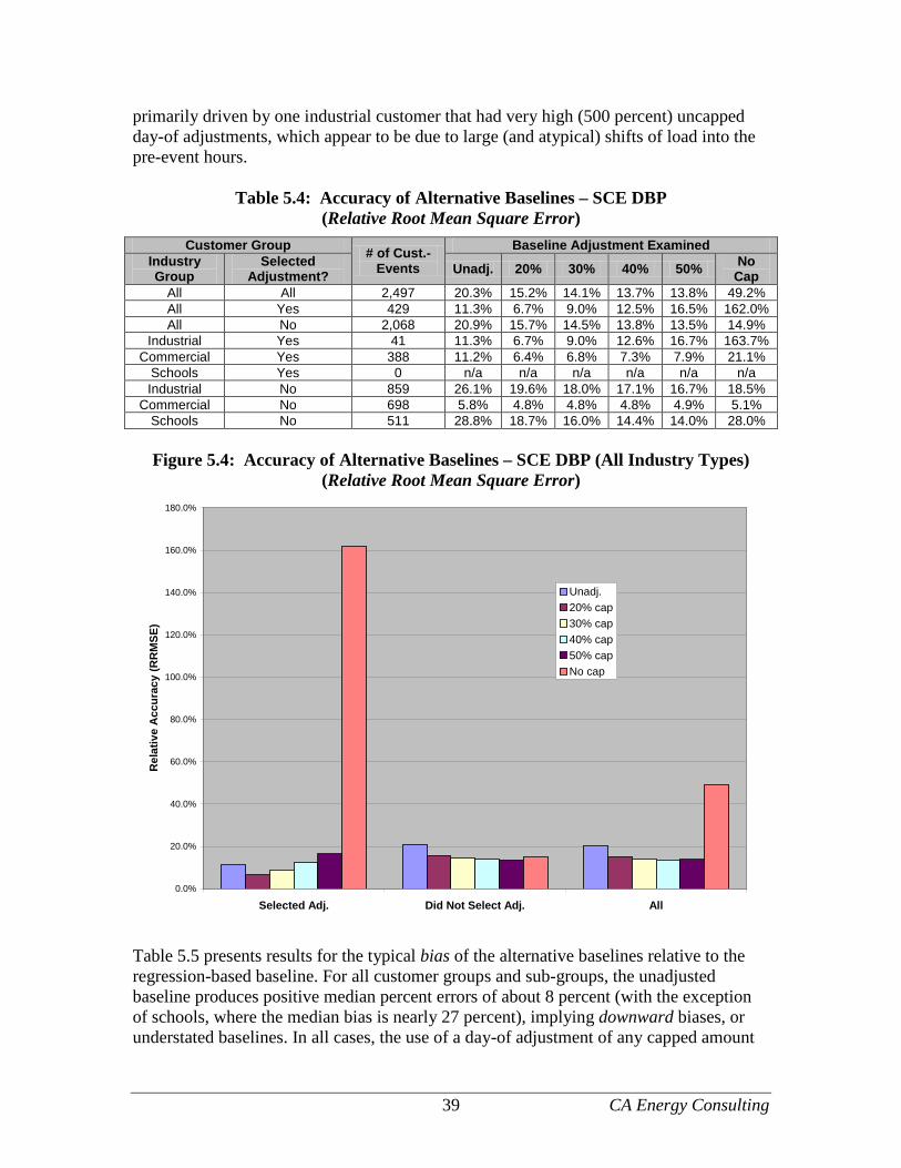
39 CA Energy Consulting
primarily driven by one industrial customer that had very high (500 percent) uncapped day-of adjustments, which appear to be due to large (and atypical) shifts of load into the pre-event hours.
Table 5.4: Accuracy of Alternative Baselines – SCE DBP (Relative Root Mean Square Error)
Customer Group # of Cust.-Events
Baseline Adjustment Examined Industry Group
Selected Adjustment? Unadj. 20% 30% 40% 50% No
Cap All All 2,497 20.3% 15.2% 14.1% 13.7% 13.8% 49.2% All Yes 429 11.3% 6.7% 9.0% 12.5% 16.5% 162.0% All No 2,068 20.9% 15.7% 14.5% 13.8% 13.5% 14.9%
Industrial Yes 41 11.3% 6.7% 9.0% 12.6% 16.7% 163.7% Commercial Yes 388 11.2% 6.4% 6.8% 7.3% 7.9% 21.1%
Schools Yes 0 n/a n/a n/a n/a n/a n/a Industrial No 859 26.1% 19.6% 18.0% 17.1% 16.7% 18.5%
Commercial No 698 5.8% 4.8% 4.8% 4.8% 4.9% 5.1% Schools No 511 28.8% 18.7% 16.0% 14.4% 14.0% 28.0%
Figure 5.4: Accuracy of Alternative Baselines – SCE DBP (All Industry Types)
(Relative Root Mean Square Error)
0.0%
20.0%
40.0%
60.0%
80.0%
100.0%
120.0%
140.0%
160.0%
180.0%
Selected Adj. Did Not Select Adj. All
Rel
ativ
e A
ccur
acy
(RR
MSE
)
Unadj.20% cap30% cap40% cap50% capNo cap
Table 5.5 presents results for the typical bias of the alternative baselines relative to the regression-based baseline. For all customer groups and sub-groups, the unadjusted baseline produces positive median percent errors of about 8 percent (with the exception of schools, where the median bias is nearly 27 percent), implying downward biases, or understated baselines. In all cases, the use of a day-of adjustment of any capped amount
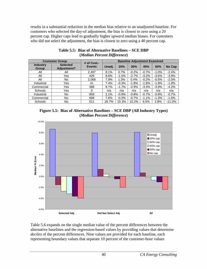
40 CA Energy Consulting
results in a substantial reduction in the median bias relative to an unadjusted baseline. For customers who selected the day-of adjustment, the bias is closest to zero using a 20 percent cap. Higher caps lead to gradually higher upward median biases. For customers who did not select the adjustment, the bias is closest to zero using a 40 percent cap.
Table 5.5: Bias of Alternative Baselines – SCE DBP (Median Percent Difference)
Customer Group # of Cust.-Events
Baseline Adjustment Examined Industry Group
Selected Adjustment? Unadj. 20% 30% 40% 50% No Cap
All All 2,497 8.1% 0.7% -0.2% -0.7% -1.0% -2.4% All Yes 429 8.6% -1.5% -2.7% -3.2% -3.6% -3.9% All No 2,068 7.9% 1.3% 0.4% -0.2% -0.5% -2.0%
Industrial Yes 41 7.4% -0.3% -1.8% -1.8% -1.8% -1.8% Commercial Yes 388 8.7% -1.7% -2.9% -3.4% -3.9% -4.2%
Schools Yes 0 n/a n/a n/a n/a n/a n/a Industrial No 859 2.1% -0.9% -0.8% -0.7% -0.8% -0.7%
Commercial No 698 7.6% -0.3% -0.7% -1.1% -1.3% -1.6% Schools No 511 26.7% 15.3% 10.2% 6.5% 2.8% -11.0%
Figure 5.5: Bias of Alternative Baselines – SCE DBP (All Industry Types)
(Median Percent Difference)
-6.0%
-4.0%
-2.0%
0.0%
2.0%
4.0%
6.0%
8.0%
10.0%
Selected Adj. Did Not Select Adj. All
Med
ian
% E
rror
Unadj.20% cap30% cap40% cap50% capNo cap
Table 5.6 expands on the single median value of the percent differences between the alternative baselines and the regression-based values by providing values that determine deciles of the percent differences. Nine values are provided for each baseline, each representing boundary values that separate 10 percent of the customer-hour values
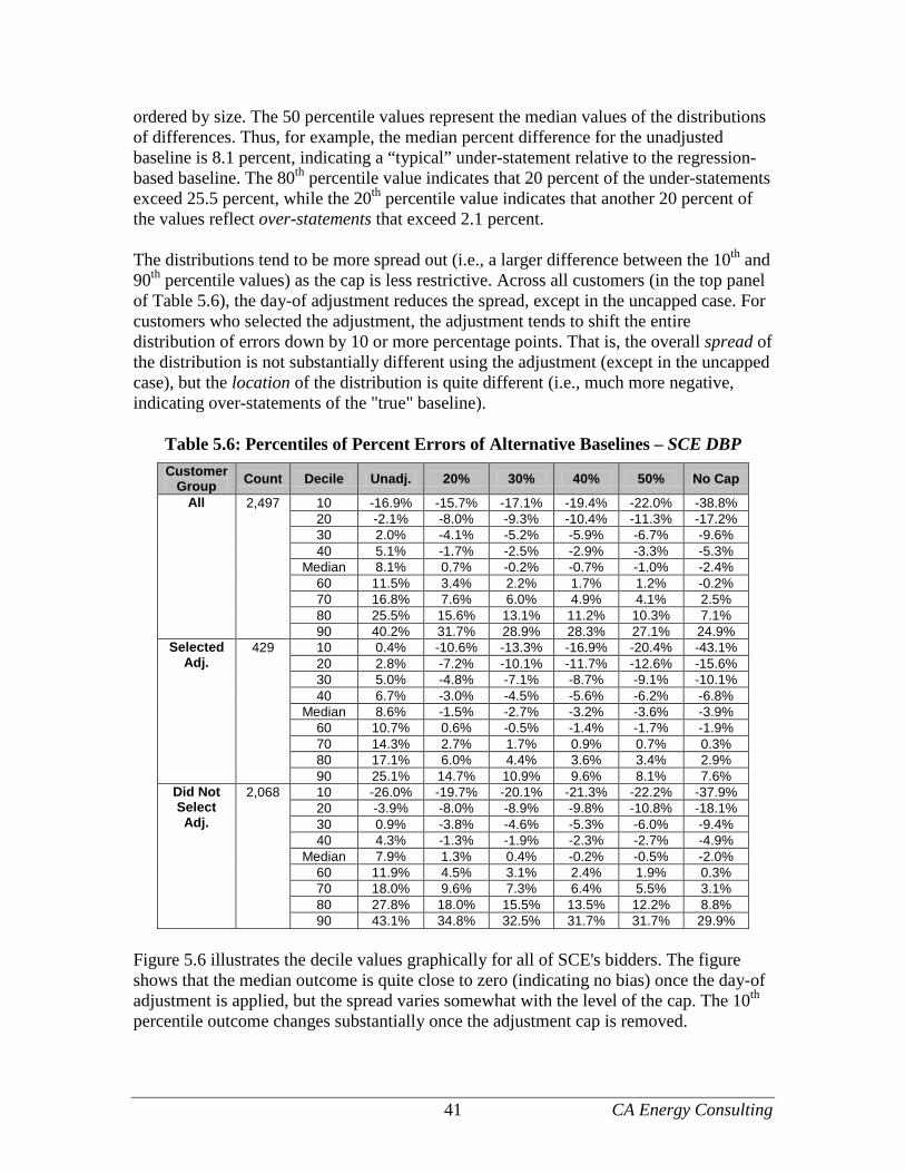
41 CA Energy Consulting
ordered by size. The 50 percentile values represent the median values of the distributions of differences. Thus, for example, the median percent difference for the unadjusted baseline is 8.1 percent, indicating a “typical” under-statement relative to the regression-based baseline. The 80th percentile value indicates that 20 percent of the under-statements exceed 25.5 percent, while the 20th percentile value indicates that another 20 percent of the values reflect over-statements that exceed 2.1 percent. The distributions tend to be more spread out (i.e., a larger difference between the 10th and 90th percentile values) as the cap is less restrictive. Across all customers (in the top panel of Table 5.6), the day-of adjustment reduces the spread, except in the uncapped case. For customers who selected the adjustment, the adjustment tends to shift the entire distribution of errors down by 10 or more percentage points. That is, the overall spread of the distribution is not substantially different using the adjustment (except in the uncapped case), but the location of the distribution is quite different (i.e., much more negative, indicating over-statements of the "true" baseline).
Table 5.6: Percentiles of Percent Errors of Alternative Baselines – SCE DBP Customer
Group Count Decile Unadj. 20% 30% 40% 50% No Cap
All 2,497 10 -16.9% -15.7% -17.1% -19.4% -22.0% -38.8% 20 -2.1% -8.0% -9.3% -10.4% -11.3% -17.2% 30 2.0% -4.1% -5.2% -5.9% -6.7% -9.6% 40 5.1% -1.7% -2.5% -2.9% -3.3% -5.3%
Median 8.1% 0.7% -0.2% -0.7% -1.0% -2.4% 60 11.5% 3.4% 2.2% 1.7% 1.2% -0.2% 70 16.8% 7.6% 6.0% 4.9% 4.1% 2.5% 80 25.5% 15.6% 13.1% 11.2% 10.3% 7.1% 90 40.2% 31.7% 28.9% 28.3% 27.1% 24.9%
Selected Adj.
429 10 0.4% -10.6% -13.3% -16.9% -20.4% -43.1% 20 2.8% -7.2% -10.1% -11.7% -12.6% -15.6% 30 5.0% -4.8% -7.1% -8.7% -9.1% -10.1% 40 6.7% -3.0% -4.5% -5.6% -6.2% -6.8%
Median 8.6% -1.5% -2.7% -3.2% -3.6% -3.9% 60 10.7% 0.6% -0.5% -1.4% -1.7% -1.9% 70 14.3% 2.7% 1.7% 0.9% 0.7% 0.3% 80 17.1% 6.0% 4.4% 3.6% 3.4% 2.9% 90 25.1% 14.7% 10.9% 9.6% 8.1% 7.6%
Did Not Select Adj.
2,068 10 -26.0% -19.7% -20.1% -21.3% -22.2% -37.9% 20 -3.9% -8.0% -8.9% -9.8% -10.8% -18.1% 30 0.9% -3.8% -4.6% -5.3% -6.0% -9.4% 40 4.3% -1.3% -1.9% -2.3% -2.7% -4.9%
Median 7.9% 1.3% 0.4% -0.2% -0.5% -2.0% 60 11.9% 4.5% 3.1% 2.4% 1.9% 0.3% 70 18.0% 9.6% 7.3% 6.4% 5.5% 3.1% 80 27.8% 18.0% 15.5% 13.5% 12.2% 8.8% 90 43.1% 34.8% 32.5% 31.7% 31.7% 29.9%
Figure 5.6 illustrates the decile values graphically for all of SCE's bidders. The figure shows that the median outcome is quite close to zero (indicating no bias) once the day-of adjustment is applied, but the spread varies somewhat with the level of the cap. The 10th percentile outcome changes substantially once the adjustment cap is removed.

42 CA Energy Consulting
Figure 5.6: Percentiles of Percent Errors of Alternative Baselines – SCE DBP
-40.0%
-30.0%
-20.0%
-10.0%
0.0%
10.0%
20.0%
30.0%
40.0%
50.0%
Unadj. 20% 30% 40% 50% No Cap
% B
asel
ine
Erro
r, by
Dec
ile
10th %ile20th %ile30th %ile40th %ileMedian60th %ile70th %ile80th %ile90th %ile
5.5 Summary of Results The baseline analysis provides strong evidence that day-of adjustments to the 10-in-10 baseline improve accuracy. For PG&E, a 30 percent adjustment cap produces the most accurate baselines. In this case, the error does not vary substantially with changes in the cap percentage. It is interesting to note that the day-of adjustment does not improve baseline accuracy for the industrial customers who have selected it. The story is somewhat different for SCE, and depends more strongly upon whether one examines all bidding customers or only bidding customers who have selected the day-of adjustment. Across all bidding customers, a 40 percent adjustment cap produces the most accurate baselines, though the error rate does not vary much with the cap level. However, removing the cap entirely produces a large reduction in baseline accuracy (this result is largely driven by the results for one large industrial customer). For customers who have selected the day-of adjustment, the variation in accuracy across alternative cap levels is larger, with a 20 percent cap level producing the most accurate baselines. Regarding bias (as measured by the median percentage error), the story differs across utilities. At PG&E, bias is slightly exacerbated by the day-of adjustment for customers who have selected it, and the bias displays little variation across the alternative cap levels. However, the results show that the day-of adjustment (at any cap level) would nearly eliminate bias for the median customer among those who have not yet selected it.

43 CA Energy Consulting
At SCE, the results indicate that bias is substantially reduced by the day-of adjustment. This is true regardless of whether the customer has selected the day-of adjustment. For customers who have selected the optional adjustment, bias is minimized with a 20 percent adjustment cap. For customers who have not yet selected the optional adjustment, bias is minimized with a 40 percent cap.
6. Ex Ante Load Impact Forecast
6.1 Ex Ante Load Impact Requirements The DR Load Impact Evaluation Protocols require that hourly load impact forecasts for event-based DR resources must be reported at the program level and by LCA for the following scenarios:
• For a typical event day in each year; and • For the monthly system peak load day in each month for which the resource is
available;
under both:
• 1-in-2 weather-year conditions, and • 1-in-10 weather-year conditions.
at both:
• the program level (i.e., in which only the program in question is called), and • the portfolio level (i.e., in which all demand response programs are called).
6.2 Description of Methods This section describes the methods used to develop the relevant groups of customers, to develop reference loads for the relevant customer types and event day-types, and to develop percentage load impacts for a typical event day.
6.2.1 Development of Customer Groups For PG&E’s program, customer accounts were assigned to one of three size groups and the relevant LCA. The three size groups were the following:
• Small – maximum demand less than 20 kW; • Medium – maximum demand between 20 and 200 kW; • Large – maximum demand greater than 200 kW.
The specific definition of “maximum demand” was based on the tariff on which the customer is served. For example, a tariff may require that a customer’s monthly peak demand exceeds 20kW during any one of the previous twelve months. The total number of customer “cells” developed is therefore equal to 24 (= 3 size groups x 8 LCAs). For SCE, the analysis is complicated by two upcoming changes to the program. In 2013, the program will begin enrolling customers with demands under 200 kW. In addition, at

44 CA Energy Consulting
the end of 2013, SCE will remove "non-performing" customers from DBP. Customers will be identified as "non-performing" if they do not receive a credit during the program year.
6.2.2 Development of Reference Loads and Load Impacts Reference loads and load impacts for all of the above factors were developed in the following series of steps:
1. Define data sources; 2. Estimate ex ante regressions and simulate reference loads by cell and scenario; 3. Calculate percentage load impacts by cell; 4. Apply percentage load impacts to the reference loads; and 5. Scale the reference loads using enrollment forecasts.
Each of these steps is described below. Define data sources For both PG&E and SCE, the reference loads and percentage load impacts are developed using data for customers enrolled in DBP during the 2011 program year, using data from the 2009 through 2011 program years. We divided the DBP customers into two groups according to whether they are dually enrolled in the Base Interruptible Program (BIP). BIP customers tend to be larger and more demand responsive (even during DBP events) than other DBP customers. For PG&E, separating the dually enrolled customers helped ensure that The Brattle Group was able to properly match enrollments to load impacts. For both PG&E and SCE, separating dually enrolled customers allowed us to produce portfolio load impacts, which are the load impacts that occur when all DR programs are simultaneously called. Specifically, when DBP and BIP events are called for the same hours, customers enrolled in both programs may not participate in the DBP event. Therefore, the portfolio load impacts for DBP exclude load impacts from customers dually enrolled in BIP. Program-level load impacts include all enrolled customers. Simulate reference loads In order to develop reference loads, we first re-estimated regression equations for each enrolled customer account, using data for program years 2009 through 2011. These equations were then used to simulate reference loads by customer type under the various scenarios required by the Protocols (e.g., the typical event day in a 1-in-2 weather year). For the summer months, the re-estimated regression equations were similar in design to the ex post load impact equations described in Section 3.2, differing in four ways. First, the ex ante models excluded the morning-usage variable. While this variable is useful for improving accuracy in estimating ex post load impacts for particular events, it complicates the use of the equations in ex ante simulation. That is, it would require a separate simulation of the level of the morning load. Second, the ex ante models excluded the summer variables (e.g., the summer variable interacted with the hourly profile).

45 CA Energy Consulting
Third, the event variables were modified from the version that produces estimates of 24 hourly load impact values for each event, to a version that produces estimates of average hourly event-period load impacts across all events. The fourth difference between the ex post and ex ante models is that the ex ante model uses separate month and year indicator variables, whereas the ex post model interacted them (such that each month and year had its own intercept). Because DBP events may be called in any month of the year, we estimated separate regression models to allow us to simulate non-summer reference loads. The non-summer model is shown below. This model is estimated separately from the summer ex ante model. It only differs from the summer model in two ways: it includes HDHt variables, where the summer model does not; and the month dummies relate to a different set of months. Table 6.1 describes the terms included in the equation.
ti
tiYEARi
iti
MONTHi
iti
DTYPEi
iti
hi
itti
FRIi
itti
MONi
itti
HDHi
itti
CDHi
ititi
BIPi
i ititi
OTHitti
DBPit
eYEARbMONTHb
DTYPEbhbFRIhb
MONhbHDHhbCDHhb
BIPEvthbOtherEvthbDBPhbaQ
+×+×+
×+×+××+
××+××+××+
××+××+××+=
∑∑
∑∑∑
∑∑∑
∑∑ ∑
=−−=
===
===
== =
)()(
)()()(
)()()(
)()()(
2011
2009,
1210,52,
5
2,
24
2,
24
2,
24
2,
24
1,
24
1,
24
1,,
24
1
24
1,,,
Table 6.1: Descriptions of Terms included in the Ex Ante Regression Equation
Variable Name Variable Description
Qt the demand in hour t for a customer enrolled in DBP prior to the last event date The various
b’s the estimated parameters
hi,t a dummy variable for hour i DBPt an indicator variable for program event days CDHt cooling degree hours HDHt heating degree hours18
OtherEvtt equals one in the event hours of other demand response programs in which the customer is enrolled
BIPEvti,t Equals one in BIP event hours if the customer is enrolled in BIP program MONt a dummy variable for Monday FRIt a dummy variable for Friday
DTYPEi,t a series of dummy variables for each day of the week MONTHi,t a series of dummy variables for each month YEARi,t a series of dummy variables for each year; and et is the error term
et the error term. 18 Heating degree hours (HDH) was defined as MAX[0, 50 – TMP], where TMP is the hourly temperature expressed in degrees Fahrenheit. Customer-specific HDH values are calculated using data from the most appropriate weather station.

46 CA Energy Consulting
Once these models were estimated, we simulated 24-hour load profiles for each required scenario. Each of the profiles was simulated as an average of Tuesday, Wednesday, and Thursday profiles. The typical event day was assumed to occur in August. Much of the differences across scenarios can be attributed to varying weather conditions. The definitions of the 1-in-2 and 1-in-10 weather years are the same as those used to develop ex ante load forecasts in the previous two studies (developed following PY2009). Calculate forecast percentage load impacts For both PG&E and SCE, the percentage load impacts were based on estimates from a model using data from program years 2009 through 2011. Specifically, we examined only customers enrolled in PY2011, but included data from the previous two program years for customers that were enrolled in those years. This method allowed us to base the ex ante load impacts on a larger sample of events, which should improve the reliability and consistency of the load impacts across forecasts. For PG&E, hourly percentage load impacts were developed by size group, LCA and whether the customer was dually enrolled in BIP. Because the forecast event window (1:00 to 6:00 p.m. in April through October; and 4:00 to 9:00 p.m. in all other months) differs from the historical event window (2:00 to 6:00 p.m.), we needed to adjust the historical percentage load impacts for use in the ex ante study. Specifically, in summer months, we shifted the load impacts back one hour beginning at hour ending 14 (1:00 to 2:00 p.m.) and replicated the hour ending 15 hour for hour ending 14. This method ensured that the load impact pattern in the pre- and post-event hours was maintained. For the non-summer months, the summer hourly percentage load impacts were shifted forward three hours, so that the event hours matched the required 4:00 to 9:00 p.m. window. We pooled customers across cells where sample sizes were small to estimate more reliable load impacts. For the DBP-only customers, the following cells were pooled:
• All under 20 kW customers; • 20 to 200 kW customers in the Greater Fresno, Humboldt, Kern, and Sierra; and • Over 200 kW customers in Humboldt and Stockton were based on an average of
all over 200 kW customers. For DBP/BIP customers, the following cells were pooled:
• All under 20 kW except those in the Greater Bay Area; • All 20 to 200 kW customers; and • Over 200 kW customers in Greater Fresno, Humboldt, Northern Coast, Sierra,
and Stockton. The uncertainty-adjusted load impacts (i.e., the 10th, 30th, 50th, 70th, and 90th percentile scenarios of load impacts) were calculated under the assumption that the load impacts are normally distributed with a mean equal to the total estimated load impact and a variance equal to the sum of the variances (the squares of the standard errors) associated with the load impact estimates.

47 CA Energy Consulting
Table 6.2 shows the average event-hour percentage load impacts used in the ex ante analysis. Note that the highest percentage load impacts occur in the DBP/BIP cells.
Table 6.2: Average Event-Hour Percentage Load Impacts by Cell, PG&E
Size Group Local Capacity Area Customer Group DBP Only DBP/BIP
Under 20 kW
Greater Bay Area 5.0% 98.7% Greater Fresno 5.0% 0.0% Humboldt 5.0% 0.0% Kern 5.0% 0.0% Northern Coast 5.0% 0.0% Other 5.0% 0.0% Sierra 5.0% 0.0% Stockton 5.0% 0.0%
20 to 200 kW
Greater Bay Area 2.8% 9.4% Greater Fresno 4.0% 9.4% Humboldt 4.0% 9.4% Kern 4.0% 9.4% Northern Coast 4.1% 9.4% Other 1.7% 9.4% Sierra 4.0% 9.4% Stockton 3.0% 9.4%
Over 200 kW
Greater Bay Area 1.3% 9.2% Greater Fresno 6.4% 1.8% Humboldt 1.9% 1.8% Kern 10.2% 21.5% Northern Coast 0.5% 1.8% Other 2.1% 32.1% Sierra 4.3% 1.8% Stockton 1.9% 1.8%
The process was somewhat different for SCE, primarily to account for program changes that will be occurring during the forecast window. First, under 200kW customers will be allowed to enroll in DBP beginning in 2013. Second, at the end of 2013, SCE plans to remove "non-performing" customers from the over 200kW group. "Non-performing" customers will be defined as those who were not paid a credit. In addition, the process needs to differentiate between customers enrolled only in DBP and those dually enrolled in DBP and BIP (to allow for the production of both portfolio- and program-based load impacts). In all cases, the SCE percentage load impacts were derived from the regression results using customers enrolled in PY2011, but including data from PY2009 and PY2010 if the customer was enrolled in those years. While we do not have estimates of the load impacts for the smaller customers to be enrolled starting in PY2013, we attempted to develop the most relevant load impact estimates from the data at hand by using only the 642 service accounts with event-day maximum demands (from our estimated reference loads) of 200kW or less. The resulting event-hour load impacts ranged from 1.3 percent to 4.6 percent.
48 CA Energy Consulting
We further differentiated customers according to whether they were dually enrolled in BIP and whether they were paid a credit in PY2011 or PY2010.19 We identified 437 service accounts that were paid a credit and 215 service accounts that were dually enrolled in BIP. The percentage load impacts were then adjusted to account for differences between the historical and ex ante event windows. The event-hour impacts were reduced from the historical eight-hour duration to the forecast five-hour duration as follows:
• The first and last event hours of the historical event window are retained as the first and last event hours of the forecast event window;
• The average of the second and third historical event hours is used as the second forecast event hour;
• The average of the fourth and fifth historical event hours is used as the third forecast event hour; and
• The average of the sixth and seventh historical event hours is used as the fourth forecast event hour.
Table 6.3 shows the average event-hour load impacts for each group.
Table 6.3: Average Event-Hour Percentage Load Impacts by Group, SCE Group Average % LI Where Used All current customers 6.3% 2012, 2013 over 200kW All current paid a credit 10.8% 2014+ over 200kW Current not in BIP 1.0% Portfolio 2012, 2013 over 200kW Not in BIP + paid a credit 1.6% Portfolio 2014+ over 200kW Under 200kW 3.0% 2013+ under 200kW
Apply percentage load impacts to reference loads for each event scenario. In this step, the percentage load impacts were applied to the reference loads for each scenario to produce all of the required reference loads, estimated event-day loads, and scenarios of load impacts. Apply forecast enrollments to produce program-level load impacts. For PG&E, The Brattle Group produced load impacts at the program level, portfolio level, and by LCA by applying the database of per-customer load impacts created in the previous step to their enrollment forecasts. The per-customer reference loads and load impacts were first scaled to match the expected size of customers (measured as annual average usage) in the enrollment forecast and then multiplied by the number of enrolled customers to obtain cell-level results. Program-level results were obtained by aggregating results across cells. SCE provided with its own enrollment forecast, which is summarized in the next section.
6.3 Enrollment Forecasts This section summarizes the enrollment forecasts, and resulting reference loads and ex ante load impact forecasts. Detailed tables of all results required by the Protocols are provided in associated appendices. 19 We included two years of data to determine "performing" customers because PY2011 contained fewer events than other program years, which may result in fewer customers being paid credits.

49 CA Energy Consulting
PG&E PG&E forecasts DBP enrollments to increase by approximately 4.9 percent in 2013, which partly consists of customers being migrated from the PeakChoice, Best Efforts program, which is closing at the end of 2012. The rate of enrollment growth declines throughout the forecast period, to 0.4 percent by 2022. By 2022, 1,329 customers are expected to be enrolled in DBP. The portfolio-based enrollment forecast includes 226 to 304 fewer customers than the program-based enrollment forecast during the summer months. Figure 6.1 illustrates PG&E's forecast enrollments in August of each year. Figure 6.1: Number of Enrolled Customers in August of Each Forecast Year, PG&E
0
200
400
600
800
1,000
1,200
1,400
2012 2013 2014 2015 2016 2017 2018 2019 2020 2021 2022
Year
Num
ber o
f Enr
olle
d C
usto
mer
s
PortfolioProgram
SCE As described earlier, SCE is planning two changes to DBP that affect the enrollment forecast. In 2013, SCE will begin enrolling customers with maximum demand under 200 kW. At the end of PY2013, SCE will remove non-performing customers from the group of over 200 kW customers. These changes are illustrated in Figure 6.1 below, which shows August enrollments by size category and forecast year. Approximately 1,100 under 200 kW customers are forecast to join DBP in 2013, and 662 over 200 kW customers are expected to be removed due to non-performance (i.e., not being paid a credit during PY2013). To account for dual enrollment, customers enrolled in DBP and BIP are removed from the program in each year to produce the portfolio-based load impacts. There are approximately 210 such customers in 2012 and 2013 and 99 customers in 2014 through 2022.

50 CA Energy Consulting
Figure 6.2: Number of Enrolled Customers in August of Each Forecast Year, SCE
0
200
400
600
800
1,000
1,200
1,400
1,600
2012 2013 2014 2015-2022
Year
Num
ber o
f Enr
olle
d C
usto
mer
s
Over 200kWUnder 200kW
6.4 Reference Loads and Load Impacts For each utility and program type, we provide the following summary information regarding the load impact forecasts, including the hourly profile of reference loads and load impacts for typical event days; the level of load impacts across years; and the distribution of load impacts by local capacity area. Outcomes for August 2014 are used throughout, as the significant program changes will have occurred by that date. Together, these figures provide a useful indication of the anticipated changes in the forecast load impacts across the various scenarios represented in the Protocol tables. All of the tables required by the Protocols are provided in an Appendix.
6.4.1 PG&E Figure 6.3 shows the program-level August 2014 forecast load impacts for a typical event day in a 1-in-2 weather year. Event-hour (1:00 to 6:00 p.m.) load impacts average 45.2 MW, which represents approximately 4.5 percent of the enrolled reference load. Figure 6.4 shows the same load impacts at the portfolio (i.e., when all DR programs are simultaneously called). On average, the load impacts are reduced by 30.5 MW (relative to the program-level load impact) to 14.8 MW. The percentage load impact goes down to 2.0 percent. The large difference between program and portfolio load impacts is due to the contribution of customers dually enrolled in DBP and BIP. In the portfolio analysis (when a BIP event is assumed to be called at the same time as the DBP event), the load impacts for the dually enrolled customers are removed from DBP, dramatically reducing the load impact.
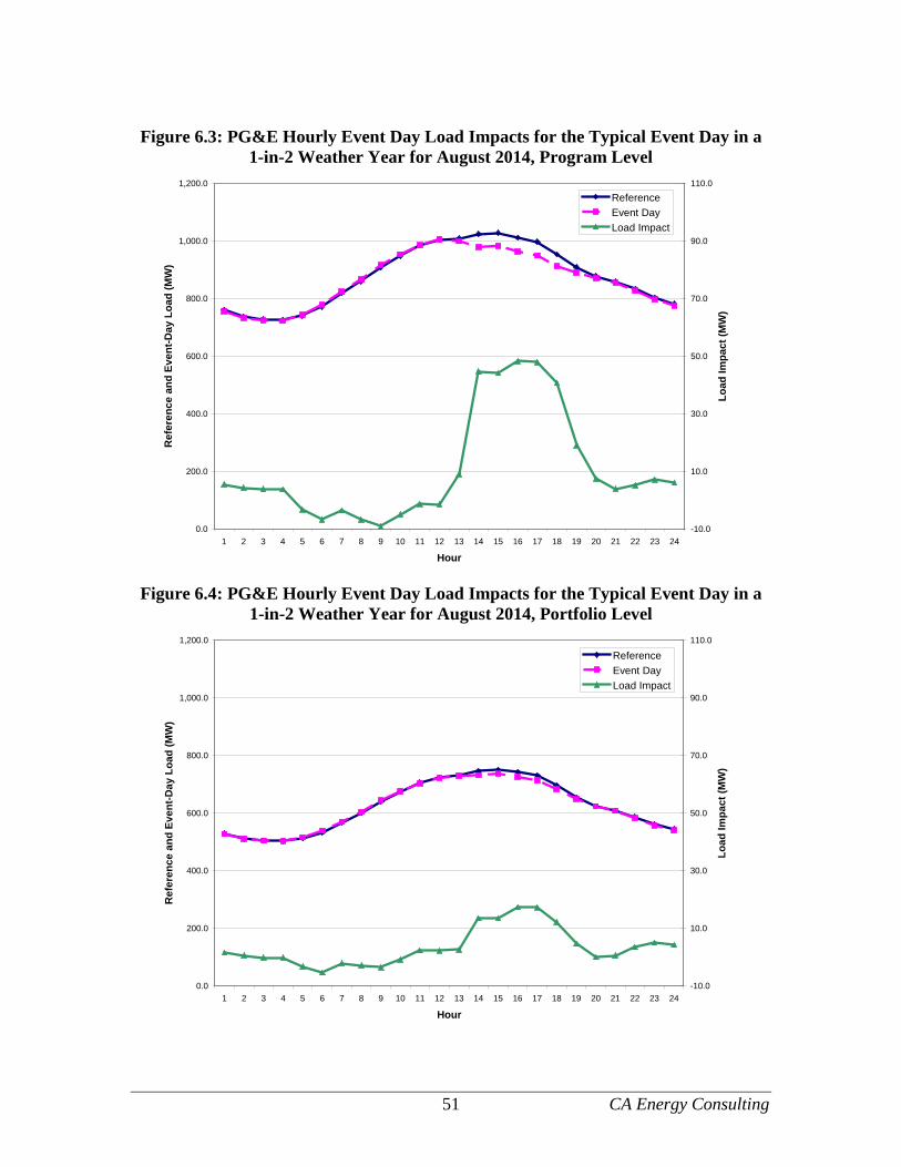
51 CA Energy Consulting
Figure 6.3: PG&E Hourly Event Day Load Impacts for the Typical Event Day in a
1-in-2 Weather Year for August 2014, Program Level
0.0
200.0
400.0
600.0
800.0
1,000.0
1,200.0
1 2 3 4 5 6 7 8 9 10 11 12 13 14 15 16 17 18 19 20 21 22 23 24
Hour
Ref
eren
ce a
nd E
vent
-Day
Loa
d (M
W)
-10.0
10.0
30.0
50.0
70.0
90.0
110.0
Load
Impa
ct (M
W)
ReferenceEvent DayLoad Impact
Figure 6.4: PG&E Hourly Event Day Load Impacts for the Typical Event Day in a
1-in-2 Weather Year for August 2014, Portfolio Level
0.0
200.0
400.0
600.0
800.0
1,000.0
1,200.0
1 2 3 4 5 6 7 8 9 10 11 12 13 14 15 16 17 18 19 20 21 22 23 24
Hour
Ref
eren
ce a
nd E
vent
-Day
Loa
d (M
W)
-10.0
10.0
30.0
50.0
70.0
90.0
110.0
Load
Impa
ct (M
W)
ReferenceEvent DayLoad Impact
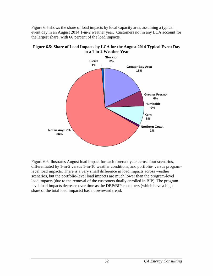
52 CA Energy Consulting
Figure 6.5 shows the share of load impacts by local capacity area, assuming a typical event day in an August 2014 1-in-2 weather year. Customers not in any LCA account for the largest share, with 66 percent of the load impacts. Figure 6.5: Share of Load Impacts by LCA for the August 2014 Typical Event Day
in a 1-in-2 Weather Year
Greater Bay Area18%
Greater Fresno6%
Humboldt0%
Kern8%
Northern Coast1%Not in Any LCA
66%
Sierra1%
Stockton0%
Figure 6.6 illustrates August load impact for each forecast year across four scenarios, differentiated by 1-in-2 versus 1-in-10 weather conditions, and portfolio- versus program-level load impacts. There is a very small difference in load impacts across weather scenarios, but the portfolio-level load impacts are much lower than the program-level load impacts (due to the removal of the customers dually enrolled in BIP). The program-level load impacts decrease over time as the DBP/BIP customers (which have a high share of the total load impacts) has a downward trend.

53 CA Energy Consulting
Figure 6.6: Average PG&E DBP Hourly Load Impacts by Scenario and Year
0.0
10.0
20.0
30.0
40.0
50.0
60.0
2012 2013 2014 2015 2016 2017 2018 2019 2020 2021 2022
Year
Ave
rage
Eve
nt-H
our L
oad
Impa
ct (M
W)
Program 1in2Portfolio 1in10Portfolio 1in2Program 1in10
6.4.2 SCE Figure 6.7 shows the program-level forecast reference loads and load impacts for an August peak day in a 1-in-2 weather year from 2015 through 2022 (the enrollment forecast is assumed to remain constant during this period of time). The average program-level load impact is 89.9 MW, or 6.6 percent of the reference load. Figure 6.8 shows the portfolio-level forecast for an August peak day in a 1-in-2 weather year from 2015 through 2022. This forecast differs from the program-level forecast by excluding customers who are dually enrolled in DBP and BIP. Because the dually enrolled customers are much more demand responsive than the non-BIP customers, the load impacts are much lower in the portfolio-based scenario. Event-hour load impacts average 11.9 MW (a reduction of 78 MW relative to the program-level load impacts), or 1.2 percent of reference load.
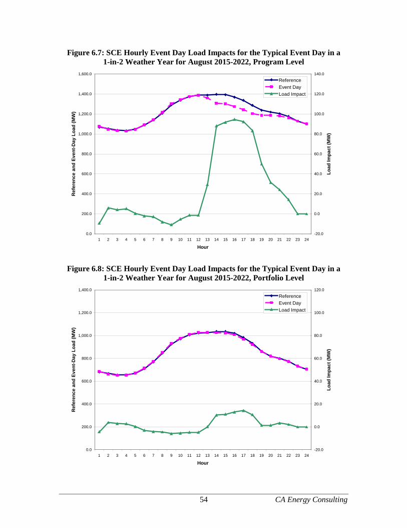
54 CA Energy Consulting
Figure 6.7: SCE Hourly Event Day Load Impacts for the Typical Event Day in a 1-in-2 Weather Year for August 2015-2022, Program Level
0.0
200.0
400.0
600.0
800.0
1,000.0
1,200.0
1,400.0
1,600.0
1 2 3 4 5 6 7 8 9 10 11 12 13 14 15 16 17 18 19 20 21 22 23 24
Hour
Ref
eren
ce a
nd E
vent
-Day
Loa
d (M
W)
-20.0
0.0
20.0
40.0
60.0
80.0
100.0
120.0
140.0
Load
Impa
ct (M
W)
ReferenceEvent DayLoad Impact
Figure 6.8: SCE Hourly Event Day Load Impacts for the Typical Event Day in a 1-in-2 Weather Year for August 2015-2022, Portfolio Level
0.0
200.0
400.0
600.0
800.0
1,000.0
1,200.0
1,400.0
1 2 3 4 5 6 7 8 9 10 11 12 13 14 15 16 17 18 19 20 21 22 23 24
Hour
Ref
eren
ce a
nd E
vent
-Day
Loa
d (M
W)
-20.0
0.0
20.0
40.0
60.0
80.0
100.0
120.0
Load
Impa
ct (M
W)
ReferenceEvent DayLoad Impact

55 CA Energy Consulting
Figure 6.9 shows the distribution of program-level load impacts across local capacity areas. The LA Basin accounts for the largest share, with 56 percent of the total load impacts.
Figure 6.9: Share of SCE DBP Load Impacts by Local Capacity Area
LA Basin56%
Outside LA Basin18%
Ventura26%
Figure 6.10 illustrates the average August hourly load impact across scenarios and year. The 1-in-10 load impacts are only slightly higher than the corresponding 1-in-2 load impacts, but the program-level load impacts are much higher than the portfolio-level load impacts. The program-level load impact rises through the forecast years, reaching 89.9 MW in the 1-in-2 load impacts for 2015-2022.
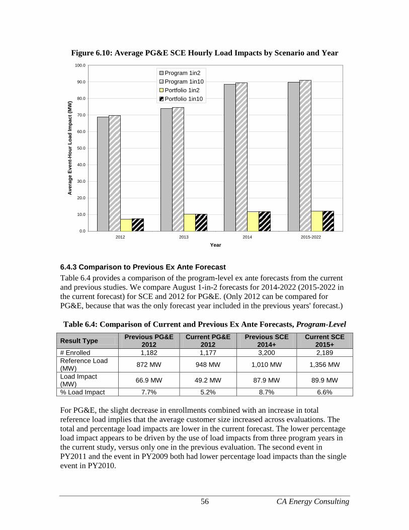
56 CA Energy Consulting
Figure 6.10: Average PG&E SCE Hourly Load Impacts by Scenario and Year
0.0
10.0
20.0
30.0
40.0
50.0
60.0
70.0
80.0
90.0
100.0
2012 2013 2014 2015-2022
Year
Ave
rage
Eve
nt-H
our L
oad
Impa
ct (M
W)
Program 1in2Program 1in10Portfolio 1in2Portfolio 1in10
6.4.3 Comparison to Previous Ex Ante Forecast Table 6.4 provides a comparison of the program-level ex ante forecasts from the current and previous studies. We compare August 1-in-2 forecasts for 2014-2022 (2015-2022 in the current forecast) for SCE and 2012 for PG&E. (Only 2012 can be compared for PG&E, because that was the only forecast year included in the previous years' forecast.) Table 6.4: Comparison of Current and Previous Ex Ante Forecasts, Program-Level
Result Type Previous PG&E 2012
Current PG&E 2012
Previous SCE 2014+
Current SCE 2015+
# Enrolled 1,182 1,177 3,200 2,189 Reference Load (MW) 872 MW 948 MW 1,010 MW 1,356 MW
Load Impact (MW) 66.9 MW 49.2 MW 87.9 MW 89.9 MW
% Load Impact 7.7% 5.2% 8.7% 6.6% For PG&E, the slight decrease in enrollments combined with an increase in total reference load implies that the average customer size increased across evaluations. The total and percentage load impacts are lower in the current forecast. The lower percentage load impact appears to be driven by the use of load impacts from three program years in the current study, versus only one in the previous evaluation. The second event in PY2011 and the event in PY2009 both had lower percentage load impacts than the single event in PY2010.

57 CA Energy Consulting
For SCE, enrollments are 1,011 lower in the current evaluation, but the total reference load is 346 MW higher and the total load impact is 2 MW higher. A few factors contribute to these differences. First, the current enrollment forecast contains a larger share of over 200 kW customers than the previous enrollment forecast (up to 43 percent from 19.2 percent). Second, the three-year perspective is used to calculate percentage load impacts, versus the one-year perspective used in the previous study. Percentage load impacts in PY2011 tended to be higher than in the previous two program years. Third, we determined "performing" customers from a different set of data. It appears that the customers identified as "performing" were larger, but had lower percentage load impacts than the customers identified as performing in the previous forecast. The effect of the shifting definition of performing customers indicates that SCE may want to use more than one year of program payments to identify performing customers. Table 6.5 conducts the same comparison, this time at the portfolio level (i.e., excluding the load impacts from customers dually enrolled in BIP). Table 6.5: Comparison of Current and Previous Ex Ante Forecasts, Portfolio-Level
Result Type Previous PG&E 2012
Current PG&E 2012
Previous SCE 2014+
Current SCE 2015+
# Enrolled 1,031 873 3,099 2,090 Reference Load (MW) 684 MW 652 MW 762 MW 1,001 MW
Load Impact (MW) 7.8 MW 12.6 MW 18.1 MW 11.9 MW
% Load Impact 1.1% 1.9% 2.4% 1.2% For PG&E, load impacts increase despite the fact that the enrollment forecast has decreased. This is due to the fact that the load response from the DBP-only customers increased substantially in PY2011 relative to PY2010. For SCE, the comparison is similar to that of the program-level described above. That is, the current forecast skews enrollments much more toward larger customers than the previous forecast. In addition, the large customers are larger than they were in the previous forecast, but with lower percentage load impacts.
7. Validity Assessment
7.1 Model Specification Tests A range of model specifications were tested before arriving at the model used in the ex post load impact analysis. Model variations included the following:
• The use of cooling degree days (CDD) versus cooling degree hours (CDH);20
20 CDD = MAX{Average(Maximum Temperature for the Day, Minimum Temperature for the Day) – Temperature Threshold,0}. CDD is the same in each hour of a given day. CDH = MAX{Temperature in that Hour – Temperature Threshold),0}. CDH can vary across the hours of a given day.

58 CA Energy Consulting
• A range of temperature thresholds used in the CDD and CDH calculations, from 50 through 70 degrees Fahrenheit in 5 degree increments;
• Whether to include the square of CDD or CDH for each hour; and
• The inclusion of the morning load variable21 versus excluding the variable and controlling for serial correlation using the Prais-Winsten estimation method.
The primary criterion used to compare the alternative specifications was the model's accuracy on a set of event-like non-event days. Testing was conducted on the aggregated DBP load for each utility. For each utility, we selected five non-event days that most resembled the actual event days to serve as proxies for event days.22 That is, the ability of the model to accurately predict the DBP load on these days may be indicative of its ability to perform well on event days (for which we do not have the "true" answer). For each utility and specification, we estimate five models. In each of these models, one of the five "test" days is withheld from the sample, and the estimated model parameters are used to predict the usage difference (i.e., the dependent variable) for that day. The difference between the observed value and the predicted value for the test days provides a means of assessing the model's accuracy. Figures 7.1 and 7.2 provide an initial examination of the appropriate temperature threshold to be used in the CDD and CDH calculations. These figures contain scatter plots of average DBP loads and temperatures for each utility, during hours ending 15 through 18 for PG&E and 13 through 20 for SCE (which encompasses all of the event hours that were called in 2011) for non-holiday and non-event weekdays in the summer of 2011. The figures appear to imply a linear relationship between temperature and load, which would lead us to suspect that the squared weather variables would have little effect on the estimates. With the exception of a couple of low-temperature days in Figure 7.1, the linear relationship holds to the lowest observed temperature levels, leading us to conclude that lower threshold temperatures are more appropriate than higher threshold temperatures. With so few observations below 60 degrees Fahrenheit, we would expect that thresholds at or below this level would produce similar results.
21 The morning load variable equals the customer's average daily load from hours ending 1 through 10. It is intended to work in a similar fashion as the day-of adjustment to the 10-in-10 baseline calculation method. 22 For PG&E, the selected days are: August 25, September 9, September 13, September 21, and September 23. For SCE, the selected days are: July 6, August 2, August 24, August 25, and September 6.
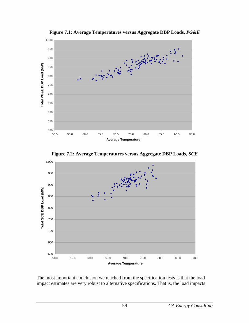
59 CA Energy Consulting
Figure 7.1: Average Temperatures versus Aggregate DBP Loads, PG&E
500
550
600
650
700
750
800
850
900
950
1,000
50.0 55.0 60.0 65.0 70.0 75.0 80.0 85.0 90.0 95.0
Average Temperature
Tota
l PG
&E
DB
P Lo
ad (M
W)
Figure 7.2: Average Temperatures versus Aggregate DBP Loads, SCE
600
650
700
750
800
850
900
950
1,000
50.0 55.0 60.0 65.0 70.0 75.0 80.0 85.0 90.0
Average Temperature
Tota
l SC
E D
BP
Load
(MW
)
The most important conclusion we reached from the specification tests is that the load impact estimates are very robust to alternative specifications. That is, the load impacts
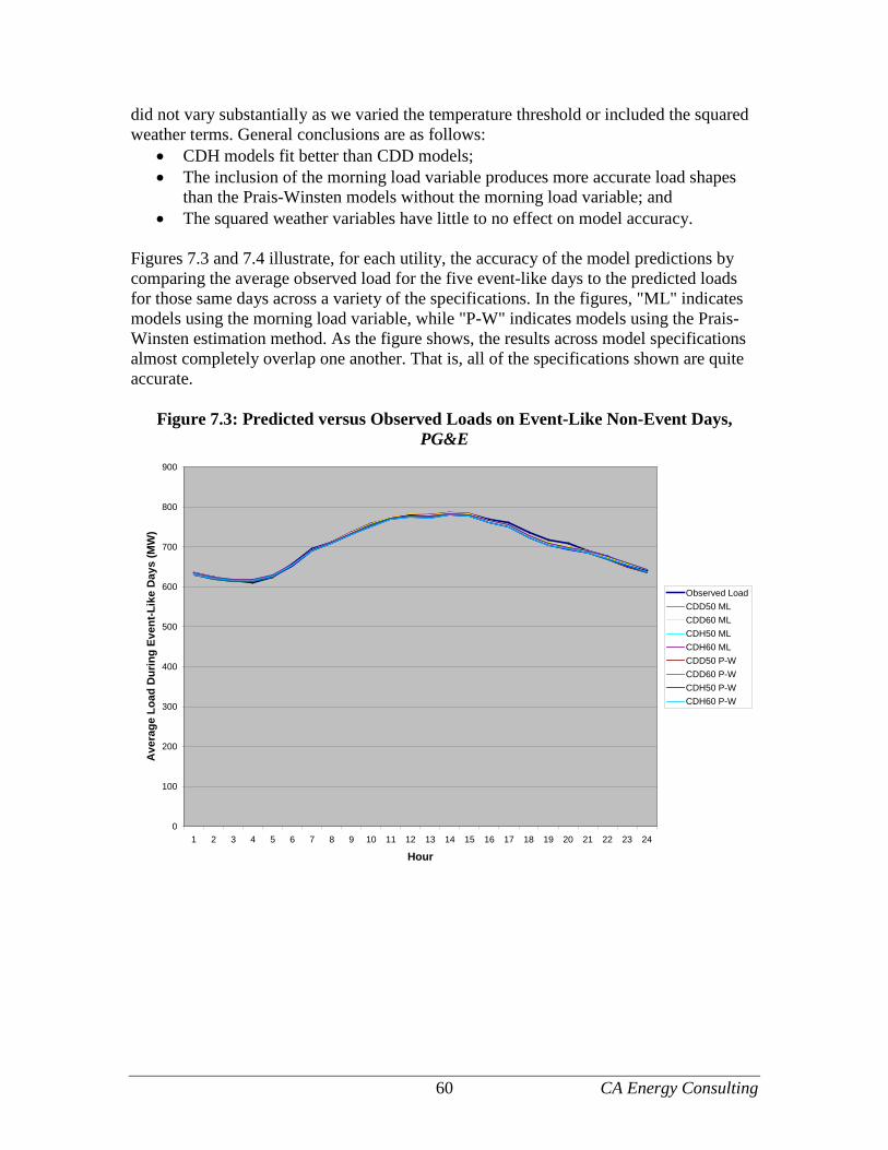
60 CA Energy Consulting
did not vary substantially as we varied the temperature threshold or included the squared weather terms. General conclusions are as follows:
• CDH models fit better than CDD models; • The inclusion of the morning load variable produces more accurate load shapes
than the Prais-Winsten models without the morning load variable; and • The squared weather variables have little to no effect on model accuracy.
Figures 7.3 and 7.4 illustrate, for each utility, the accuracy of the model predictions by comparing the average observed load for the five event-like days to the predicted loads for those same days across a variety of the specifications. In the figures, "ML" indicates models using the morning load variable, while "P-W" indicates models using the Prais-Winsten estimation method. As the figure shows, the results across model specifications almost completely overlap one another. That is, all of the specifications shown are quite accurate.
Figure 7.3: Predicted versus Observed Loads on Event-Like Non-Event Days, PG&E
0
100
200
300
400
500
600
700
800
900
1 2 3 4 5 6 7 8 9 10 11 12 13 14 15 16 17 18 19 20 21 22 23 24
Hour
Ave
rage
Loa
d D
urin
g Ev
ent-L
ike
Day
s (M
W)
Observed LoadCDD50 MLCDD60 MLCDH50 MLCDH60 MLCDD50 P-WCDD60 P-WCDH50 P-WCDH60 P-W

61 CA Energy Consulting
Figure 7.4: Predicted versus Observed Loads on Event-Like Non-Event Days, SCE
0
100
200
300
400
500
600
700
800
900
1 2 3 4 5 6 7 8 9 10 11 12 13 14 15 16 17 18 19 20 21 22 23 24
Hour
Ave
rage
Loa
d D
urin
g Ev
ent-L
ike
Day
s (M
W)
Observed LoadCDD50 MLCDD60 MLCDH50 MLCDH60 MLCDD50 P-WCDD60 P-WCDH50 P-WCDH60 P-W
Tables 7.1 and 7.2 provide detailed results from the specification tests. Model variations shown in the table include the morning load versus Prais-Winsten models; the use of CDD or CDH weather variables; and temperature thresholds of 50, 55, 60, and 65 degrees Fahrenheit. The types of results shown are the R-squared for the model as a whole; and the root mean squared error (RMSE) for all hours and the "event" hours of the event-like non-event days. The "best" value in each column is highlighted in bold. Notice that the most accurate models are nearly all in the morning load, CDH results section. Based on these results, we proceeded with the model that uses the 50 degree threshold, which produced the best fit across all hours for both utilities.
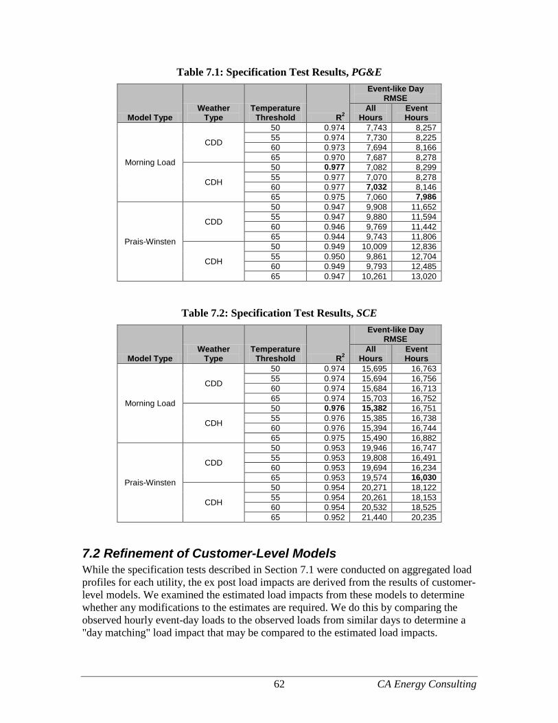
62 CA Energy Consulting
Table 7.1: Specification Test Results, PG&E
Model Type Weather
Type Temperature
Threshold R2
Event-like Day RMSE
All Hours
Event Hours
Morning Load
CDD
50 0.974 7,743 8,257 55 0.974 7,730 8,225 60 0.973 7,694 8,166 65 0.970 7,687 8,278
CDH
50 0.977 7,082 8,299 55 0.977 7,070 8,278 60 0.977 7,032 8,146 65 0.975 7,060 7,986
Prais-Winsten
CDD
50 0.947 9,908 11,652 55 0.947 9,880 11,594 60 0.946 9,769 11,442 65 0.944 9,743 11,806
CDH
50 0.949 10,009 12,836 55 0.950 9,861 12,704 60 0.949 9,793 12,485 65 0.947 10,261 13,020
Table 7.2: Specification Test Results, SCE
Model Type Weather
Type Temperature
Threshold R2
Event-like Day RMSE
All Hours
Event Hours
Morning Load
CDD
50 0.974 15,695 16,763 55 0.974 15,694 16,756 60 0.974 15,684 16,713 65 0.974 15,703 16,752
CDH
50 0.976 15,382 16,751 55 0.976 15,385 16,738 60 0.976 15,394 16,744 65 0.975 15,490 16,882
Prais-Winsten
CDD
50 0.953 19,946 16,747 55 0.953 19,808 16,491 60 0.953 19,694 16,234 65 0.953 19,574 16,030
CDH
50 0.954 20,271 18,122 55 0.954 20,261 18,153 60 0.954 20,532 18,525 65 0.952 21,440 20,235
7.2 Refinement of Customer-Level Models While the specification tests described in Section 7.1 were conducted on aggregated load profiles for each utility, the ex post load impacts are derived from the results of customer-level models. We examined the estimated load impacts from these models to determine whether any modifications to the estimates are required. We do this by comparing the observed hourly event-day loads to the observed loads from similar days to determine a "day matching" load impact that may be compared to the estimated load impacts.
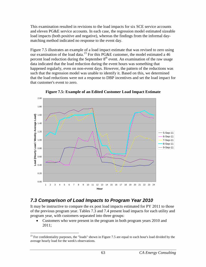
63 CA Energy Consulting
This examination resulted in revisions to the load impacts for six SCE service accounts and eleven PG&E service accounts. In each case, the regression model estimated sizeable load impacts (both positive and negative), whereas the findings from the informal day-matching method indicated no response to the event day. Figure 7.5 illustrates an example of a load impact estimate that was revised to zero using our examination of the load data.23 For this PG&E customer, the model estimated a 46 percent load reduction during the September 8th event. An examination of the raw usage data indicated that the load reduction during the event hours was something that happened regularly, even on non-event days. However, the pattern of the reductions was such that the regression model was unable to identify it. Based on this, we determined that the load reductions were not a response to DBP incentives and set the load impact for that customer's event to zero.
Figure 7.5: Example of an Edited Customer Load Impact Estimate
0.00
0.20
0.40
0.60
0.80
1.00
1.20
1.40
1.60
1.80
2.00
1 2 3 4 5 6 7 8 9 10 11 12 13 14 15 16 17 18 19 20 21 22 23 24
Hour
Load
(Hou
rly L
oad
/ Wee
kly
Ave
rage
Loa
d)
5-Sep-116-Sep-117-Sep-118-Sep-119-Sep-11
7.3 Comparison of Load Impacts to Program Year 2010 It may be instructive to compare the ex post load impacts estimated for PY 2011 to those of the previous program year. Tables 7.3 and 7.4 present load impacts for each utility and program year, with customers separated into three groups:
• Customers who were present in the program in both program years 2010 and 2011;
23 For confidentiality purposes, the "loads" shown in Figure 7.5 are equal to each hour's load divided by the average hourly load for the week's observations.

64 CA Energy Consulting
• Customers who were present in the program in PY 2011 only (new additions); and
• Customers who were present in the program in PY 2010 only (attrition). Table 7.3 shows that for PG&E the largest source of the change in load impact estimates across years is a change in estimated load impacts for customers present in both program years. However, we estimated 67.2 MW of load impacts for the first event in PY 2011, which is quite close to the value for the single test event in PY 2010. Therefore, the difference in average load impacts across years may simply reflect variability in load impacts across the two PG&E test events. Table 7.3: Comparison of Load Impacts (in MW) in PY 2010 and PY 2011, PG&E
Program Year
LI in PY 2011 LI in PY 2010 Change
In both years 55.6 66.1 -10.5 In PY 2011 only 1.3 n/a 1.3 In PY 2010 only n/a 2.1 -2.1 TOTAL 56.9 68.2 -11.3
Table 7.4 shows that for SCE the largest source of the change in load impact estimates across years is 16.3 MW in load impacts from newly enrolled customers. Therefore, the increase in program-level load impacts appears to be largely due to changes in program participation.
Table 7.4: Comparison of Load Impacts (in MW) in PY 2010 and PY 2011, SCE Program Year
LI in PY 2011 LI in PY 2010 Change
In both years 61.5 59.6 1.9 In PY 2011 only 16.3 n/a 16.3 In PY 2010 only n/a 2.5 -2.5 TOTAL 77.8 62.1 15.6
8. Recommendations We recommend an investigation of alternative methods for estimating the incremental load impacts from the AutoDR and TA/TI programs. As described in Section 4.3, data limitations prevented us from estimating reliable incremental load impacts for this evaluation. In the future, utilities may want to investigate the feasibility of basing the incremental load impacts on information gathered from data loggers applied to the equipment affected by AutoDR or TA/TI. (This may not be possible, depending on the program or specific application of the technology.) A simulated event test could be conducted before and after the technology is installed at the customer's site. A comparison of the test results before and after the installation of the technology would provide the estimate of incremental load impacts of the technology for that customer.

65 CA Energy Consulting
In addition, the utilities may want to consider whether the analysis of AutoDR and TA/TI load impacts should be conducted under a separate contract from the current load impact evaluations, such that all AutoDR and TA/TI customers would be evaluated by the same contractor using a uniform methodology. This may more easily allow the contractor to employ methods that fundamentally differ from the methods used to estimate program load impacts. One potential problem with this approach is that it may require the contractor to be familiar with the details of a variety of DR programs.
Appendices The following Appendices accompany this report. Each is an Excel file that can produce the tables required by the Protocols. DBP Study Appendix A PG&E Ex-Post Load Impact Tables DBP Study Appendix B SCE Ex-Post Load Impact Tables DBP Study Appendix C PG&E Ex-Ante Load Impact Tables DBP Study Appendix D SCE Ex-Ante Load Impact Tables