2010 Ohio UTC Student Research Conference  

   Abstract Summaries 

November 12, 2010 

The University of Akron Student Union 

Akron, Ohio 

Acknowledgements 

 Sponsors:  

Ohio Transportation Consortium, Dr. Ping Yi, Director The University of Akron Akron, Ohio 44325‐6106 330‐972‐6543 330‐972‐5449 (fax) otc@uakron.edu www.otc.uakron.edu  Center for Transportation and Materials Engineering, Joann Esenwein, Director Youngstown State University Moser Hall 2055 Youngstown, Ohio 44555 330‐941‐2421 ctme@ysu.edu http://stem.ysu.edu/CTME  Intermodal Transportation Institute, Richard Martinko, P.E., Director The University of Toledo Research and Technology Complex ‐ R1 2801 W. Bancroft Street, Mail Stop 218 Toledo, OH 43606‐3390 419‐530‐5221 419‐530‐7246 (fax) www.utoledo.edu/research/iti  

University Transportation Center ‐ Cleveland State University, Dr. Stephen Duffy, Director Fenn College of Engineering Cleveland State University 2121 Euclid Ave. SH 107 Cleveland, Ohio 44115‐2214 216‐687‐3874 216‐687‐5395 (fax) S.duffy@csuohio.edu www.csuohio.edu/engineering/utc 

Contents 

 

Bicycle‐Sharing in a College Environment……………………………………………………………………………. 

Comparison of Advance Dilemma Zone Protection Algorithms………………………………………....… 

Causes of Bumps at Pavement‐Bridge Interface………………………………………………..……………...… 

Safety Evaluation of Diamond‐Grade vs. High‐Intensity Sheeting for Work Zone Drums……... 

Coupled Thermo‐hydro‐mechanical Model for Pavement Under Frost Action……………..…...… 

University of Toledo Solar Car Project…………………………………………………………………..………..…… 

An Innovative Method for Soil Water Characteristic Curve Measurement with a         Thermo‐TDR Sensor……………………………………………………………………………………………..…...… 

Laboratory Experiments on the Variation of Hydraulic Roughness in Partially Filled Culverts   for Fish Passage Deign………………………………………….………………………………………….……..…... 

Estimating On‐Road Mobile Source Pollution in Ohio……………...…………………………………..……… 

Traffic Data Collection Using Multi‐Touch Technology on Mobile Device…………………....……… 

Effects of Left‐Side Ramps on Crash Frequency on Urban Freeway Segments………...…………… 

Evaluating Traffic Safety Behaviors of College Students…………………………………..…………...….… 

Dynamic Dilemma Zone at Signalized Intersections: Safety Issue and Solutions……...………..… 

Estimating Vehicle Length under Traffic Congestion……………………………………...………...………… 

Using Dataming in Classifications of Traffic Counting Locations: A Case Study in Ohio……….. 

Studies of Novel Ceramic Materials as Precursors for Preparation of Ceramic‐Metallic   Composites for Lightweight Vehicle Braking Systems (poster)…..…………………………………. 

 

 

 

1 

2 

10 

14 

15 

18 

 21 

 23 

27 

30 

32 

36 

37 

43 

46 

 49 

1

Bicycle‐Sharing in a College Environment 

Megan Petroski, Graduate Student, Kent State University  Abstract Summary 

Bike sharing  is an effective way of providing access  to sustainable modes of  transportation  to a 

large population. This stems from a desire by the campus community to begin a bike‐sharing program 

that moves  students,  faculty,  staff,  and  community members  from  one  place  to  another.  Current 

transportation patterns on the Kent State University campus and within the city of Kent demonstrate 

that bike‐sharing has a great deal of potential. Based on a web survey administered  last year, about 

60% of Kent  State University  students do not have  access  to working bikes. This  represents a  large 

population  of  potential  users.  To  address  this  issue,  Kent  State  recently  began  a  pilot  program  – 

FlashFleet ‐ with fifty bikes in six locations around campus. Our efforts are now focused on expanding 

the program to meet this demand as well as to move towards an automated system which would make 

checking bicycles out more convenient for users. 

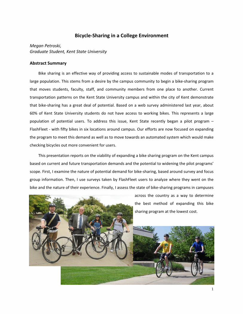
This presentation reports on the viability of expanding a bike sharing program on the Kent campus 

based on current and future transportation demands and the potential to widening the pilot programs’ 

scope. First, I examine the nature of potential demand for bike‐sharing, based around survey and focus 

group  information. Then,  I use surveys  taken by FlashFleet users  to analyze where  they went on  the 

bike and the nature of their experience. Finally, I assess the state of bike‐sharing programs in campuses 

across  the  country  as  a way  to  determine 

the  best  method  of  expanding  this  bike 

sharing program at the lowest cost.  

 

  

 

2

Comparison of Advance Dilemma Zone Protection Algorithms 

Sai Geetha.K Graduate Student, Department of Civil Engineering, University of Akron 

Abstract 

High  speed  signalized  intersections  involve  some  safety problems  in  addition  to operation  and 

design  issues. One of  the most  important safety problems at  the high speed  intersection  is dilemma 

zone protection. Dilemma zone come  into existence when the vehicle  is approaching the  intersection 

at the end of the green phase. The advance dilemma zone protection system  increases the safety at 

the  intersection  by  changing  traffic  timing  to  reduce  the  number  of  vehicles  entering  the  dilemma 

zone. This may reduce rare end and angle crashes at the intersection. 

Introduction 

The yellow phase dilemma is one of the major contributing factors to intersection related crashes, 

particularly  the  rear  end  and  right  angle  crashes.  The  so  called  dilemma  is  reflective  to  drivers’ 

indecisiveness when making  stop/pass  decisions  in  response  to  yellow  indications.  This  dilemma  is 

usually characterized by a physical zone  in advance of  the  intersection, which  is  termed as dilemma 

zone (DZ). The concept of dilemma zone was  initially proposed by Gazis et al. as a roadway segment 

within which a vehicle approaching an  intersection during the yellow  interval can neither safely clear 

the intersection, nor comfortably stop before the stop line.  

A driver approaching a signalized intersection as the light turns yellow will either have to stop or 

proceed  through  the  intersection.  If  the driver decided  to  stop,  the distance  required  to  safely  stop 

before entering the intersection is known as the stop zone (represented by Xs, in the figure below) and 

is defined as 

where:

       v = vehicle approach speed (ft/sec) 

  t = driver perception reaction time (sec) 

  g = acceleration of gravity (ft/sec2) 

  f = coefficient of friction 

  G = roadway gradient (%/100) 

3

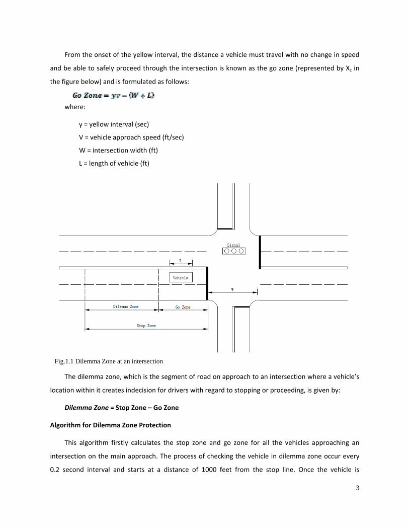
From the onset of the yellow interval, the distance a vehicle must travel with no change in speed 

and be able to safely proceed through the  intersection  is known as the go zone (represented by Xc  in 

the figure below) and is formulated as follows: 

where: 

  y = yellow interval (sec) 

  V = vehicle approach speed (ft/sec) 

  W = intersection width (ft) 

  L = length of vehicle (ft) 

The dilemma zone, which is the segment of road on approach to an intersection where a vehicle’s 

location within it creates indecision for drivers with regard to stopping or proceeding, is given by: 

Dilemma Zone = Stop Zone – Go Zone 

Algorithm for Dilemma Zone Protection 

This  algorithm  firstly  calculates  the  stop  zone  and  go  zone  for  all  the  vehicles  approaching  an 

intersection on the main approach. The process of checking the vehicle  in dilemma zone occur every 

0.2  second  interval  and  starts  at  a  distance  of  1000  feet  from  the  stop  line.  Once  the  vehicle  is 

Fig.1.1 Dilemma Zone at an intersection

4

confirmed  that  it will be  in dilemma  zone  in 1  second,  the green  signal  is extended by 1  second  to 

protect this vehicle as it enters. The extension described above occurs only when there is a conflicting 

call from the minor approach. This algorithm checks the nearest vehicle to stop line, to see if it is in 

Dilemma Zone or not, and extends green accordingly. This algorithm terminates the green only if, there 

is no vehicle in the dilemma zone or if max‐out occurs. 

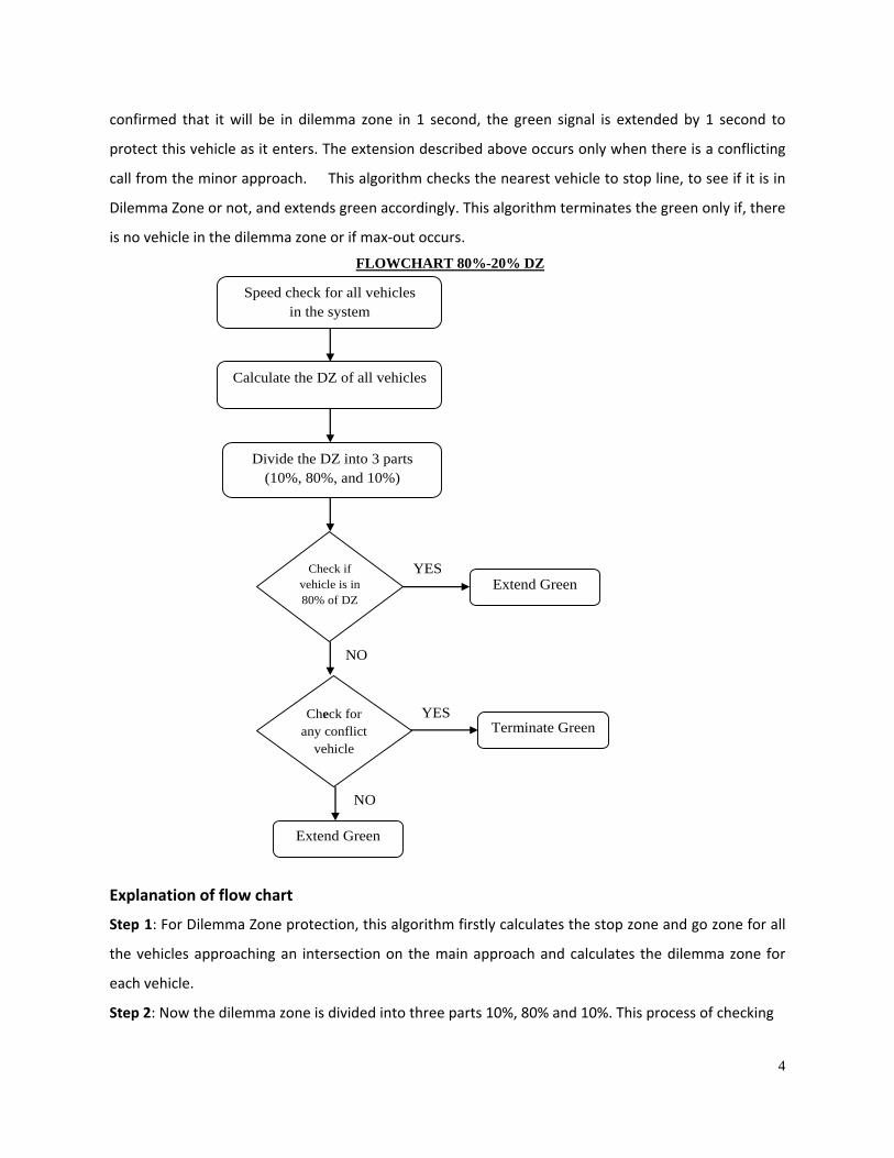
Explanation of flow chart 

Step 1: For Dilemma Zone protection, this algorithm firstly calculates the stop zone and go zone for all 

the vehicles approaching an  intersection on  the main approach and calculates  the dilemma zone  for 

each vehicle. 

Step 2: Now the dilemma zone is divided into three parts 10%, 80% and 10%. This process of checking  

  Speed check for all vehicles in the system

Calculate the DZ of all vehicles

Divide the DZ into 3 parts (10%, 80%, and 10%)

Check for any conflict

vehicle

Extend Green Check if

vehicle is in 80% of DZ

Terminate Green

Extend Green

YES

YES

NO

NO

FLOWCHART 80%-20% DZ

5

the vehicle in dilemma zone occur every 0.2sec interval and starts at a distance of 1000 feet from the 

stop line 

Step 3: The system first checks if the vehicle is in the 80% of the dilemma zone, 

(i)  If “yes” it will extend green. 

 (ii)  If “no”, then the system again checks for any conflict call from the other approach .If there is    

any conflict call then it terminates green or else extend green. 

This algorithm checks the nearest vehicle to stop  line, to see  if  it  is  in Dilemma Zone or not, and 

extends green accordingly. 

  Speed check for all vehicles in the system

Calculate the DZ of all vehicles

Divide the DZ into 3 parts (25%, 25%, and 50%)

Check for any conflict

vehicle

Extend Green If vehicle is

in 50% of DZ

Terminate Green

If vehicle is in 50% -

75%of DZ

Check for any conflict

vehicle

Extend Green

YES

YES

NO

YES

NO

NO

YES

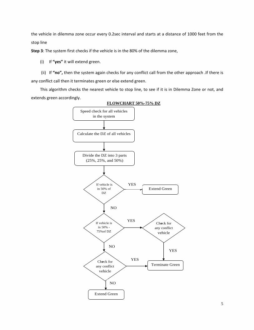
FLOWCHART 50%-75% DZ

6

Explanation of flow chart 

Step 1: For Dilemma Zone protection, this algorithm firstly calculates the stop zone and go zone 

for all the vehicles approaching an intersection on the main approach and calculates the dilemma zone 

for each vehicle. 

Step  2: Now  the dilemma  zone  is divided  into  three parts 25%, 25%  and 50%. This process of 

checking the vehicle in dilemma zone occur every 0.2 sec interval and starts at a distance of 1000 feet 

from the stop line 

Step 3: The system first checks if the vehicle is in the 50% of the dilemma zone, 

(i)    If “yes” it will extend green. 

(ii)   If “no” then the system will again check if there is any vehicle in the 50‐75% of the dilemma           

       zone. 

(a)  If “yes” then it will check if there is any conflict calls from the other approach, if vehicle is  

    present then it will terminate green or else extend green. 

(b)  If “no”, then the system again checks for any conflict call from the other approach .If there is    

    any conflict call then it terminates green or else extend green. 

This algorithm checks the nearest vehicle to stop  line, to see  if  it  is  in Dilemma Zone or not, and 

extends green accordingly. 

Comparison between the 50‐75% Dilemma Zone and 20‐80% Dilemma Zone Algorithm 

For comparing these two advance dilemma zone protection algorithms, an intersection was drawn 

in VISSIM  (having major  and minor  road). The  following  combination of  the  volumes  for major and 

minor were used for various simulation runs: 

 

Volume Major Road Volume Minor Road

300 400

600 400

900 400

1200 400

300 200

600 200

900 200

1200 200

7

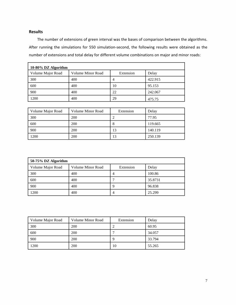
Results 

The number of extensions of green interval was the bases of comparison between the algorithms. 

After  running  the  simulations  for 550  simulation‐second,  the  following  results were obtained as  the 

number of extensions and total delay for different volume combinations on major and minor roads: 

10-80% DZ Algorithm

Volume Major Road Volume Minor Road Extension Delay

300 400 4 422.915

600 400 10 95.153

900 400 22 242.067

1200 400 29 475.75

Volume Major Road Volume Minor Road Extension Delay

300 200 2 77.95

600 200 8 119.665

900 200 13 140.119

1200 200 13 250.139

50-75% DZ Algorithm

Volume Major Road Volume Minor Road Extension Delay

300 400 4 100.86

600 400 7 35.8731

900 400 9 96.838

1200 400 4 25.299

Volume Major Road Volume Minor Road Extension Delay

300 200 2 60.95

600 200 7 34.057

900 200 9 33.794

1200 200 10 55.265

8

 

 

 

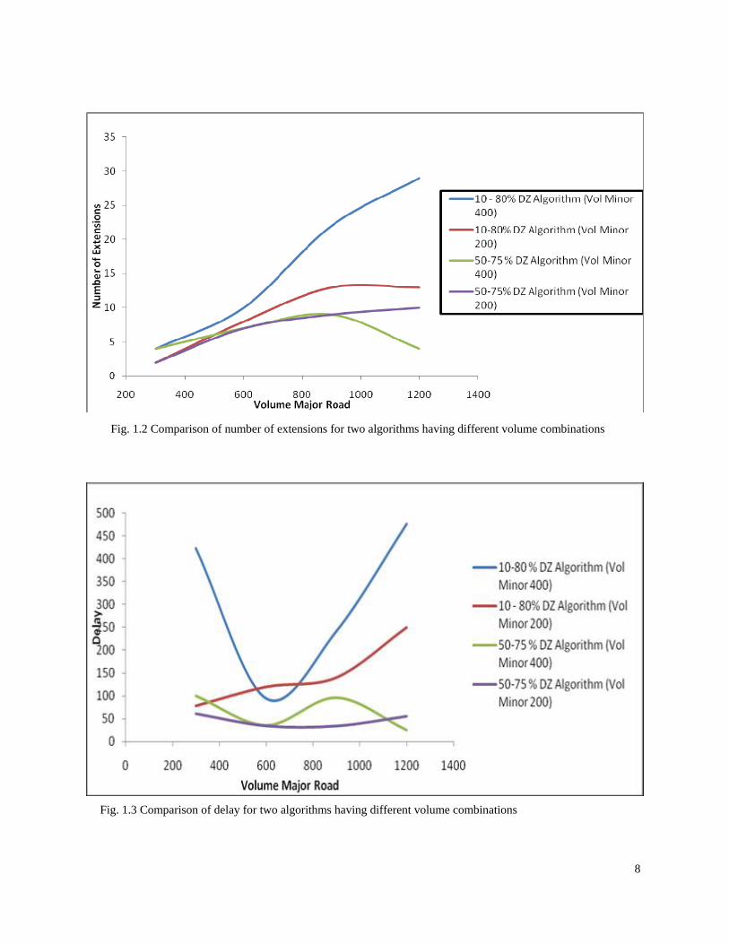
Fig. 1.2 Comparison of number of extensions for two algorithms having different volume combinations

Fig. 1.3 Comparison of delay for two algorithms having different volume combinations

9

Conclusion 

It’s quite evident from the Fig .1.2 above that there is difference between numbers of extensions 

in both the cases. The number of extensions  in 10‐80% algorithm  is much higher as compared to 50‐

75% algorithm, when volume on major road  is  increased. This may be due  to reason  that  in 10‐80% 

algorithm, the Dilemma Zone  is shortened by 20 % whereas  in 50‐75% algorithm the  last 25 % of Di‐

lemma Zone is always neglected for extensions i.e. dilemma zone is always shortened for 25% or more. 

Hence, less number of vehicles falls in shortened dilemma zone for which extension can occur. 

Fig. 1.3 shows that there is no relationship between the volume on major road and delay, this may 

be because of the reason that simulations ran with combination of volume (major and minor road vol‐

ume) were just ran for one time and that too for small time period of 550 simulation‐seconds. 

10

Causes of Bumps at Pavement‐Bridge Interface 

AKM Anwarul Islam, PhD., P.E. Associate Professor, Civil & Environmental Engineering, Youngstown State University  Amar Shukla Graduate Student, Civil & Environmental Engineering, Youngstown State University,  Summary 

This  research was performed  to determine  the probable causes and cost‐effective  solutions  for 

reducing bumps  at pavement‐bridge  interface. Bumps  can be defined  as  the differential  settlement 

between a bridge and an approach slab. Approach slabs are provided for better transition of vehicles. 

Briaud et al.  (1997) summarized that out of 600,000 bridges across the United States; approximately 

150,000 bridges have bumps that cost approximately $100 million annually for repair. Bumps not only 

cause discomforts to riders but also create bad images of transportation departments.  

A thorough study of previous research work were conducted and various causes of bumps were 

found, which were: movement of  soil beneath  the  slab,  strength deficient approach  slabs, continual 

impact of vehicles running over already compacted area,  insufficient compaction of soil especially of 

the embankment backfill,  types of  soil,  short‐term and  long‐term  settlement, bridge end conditions, 

construction methods, roadway paving and bridge/roadway joint, water seepage and traffic volume. 

This research was based on two major causes of bridge bumps which are movement/settlement 

of  soil  under  the  approach  slab  and  insufficient  strength  of  an  approach  slab.    Experimental 

investigations were conducted on 2 bridges with bumps and 3 bridges without bumps at Columbiana 

County  in Ohio. Soil was collected from the surface and Sieve Analysis tests and Atterberg Limit tests 

(Liquid Limit and Plastic Limit) were performed. Soil was classified according to AASHTO Standards as 

shown in Table 1.1. It was found that the soil is granular for all the sites and various methods through 

which proper compaction of granular soil can be obtained are pneumatic rubber‐tired rollers, vibratory 

rollers and handheld vibrating plates. 

Standard  drawings  of  different  State  Departments  of  Transportation  (DOTs) were  studied  and 

respective  strengths  of  approach  slabs  of  those DOTs were  determined  as  shown  in  Table  1.2.  For 

calculations slab was considered as doubly reinforced and simply supported.  

 

11

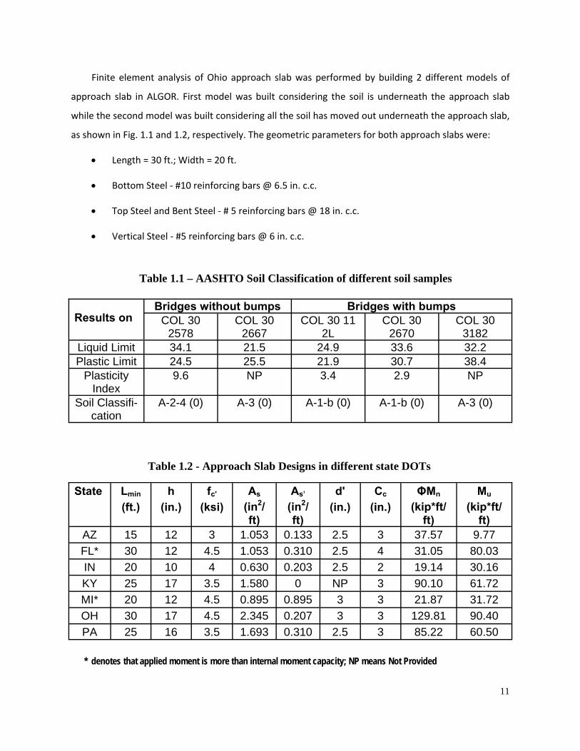
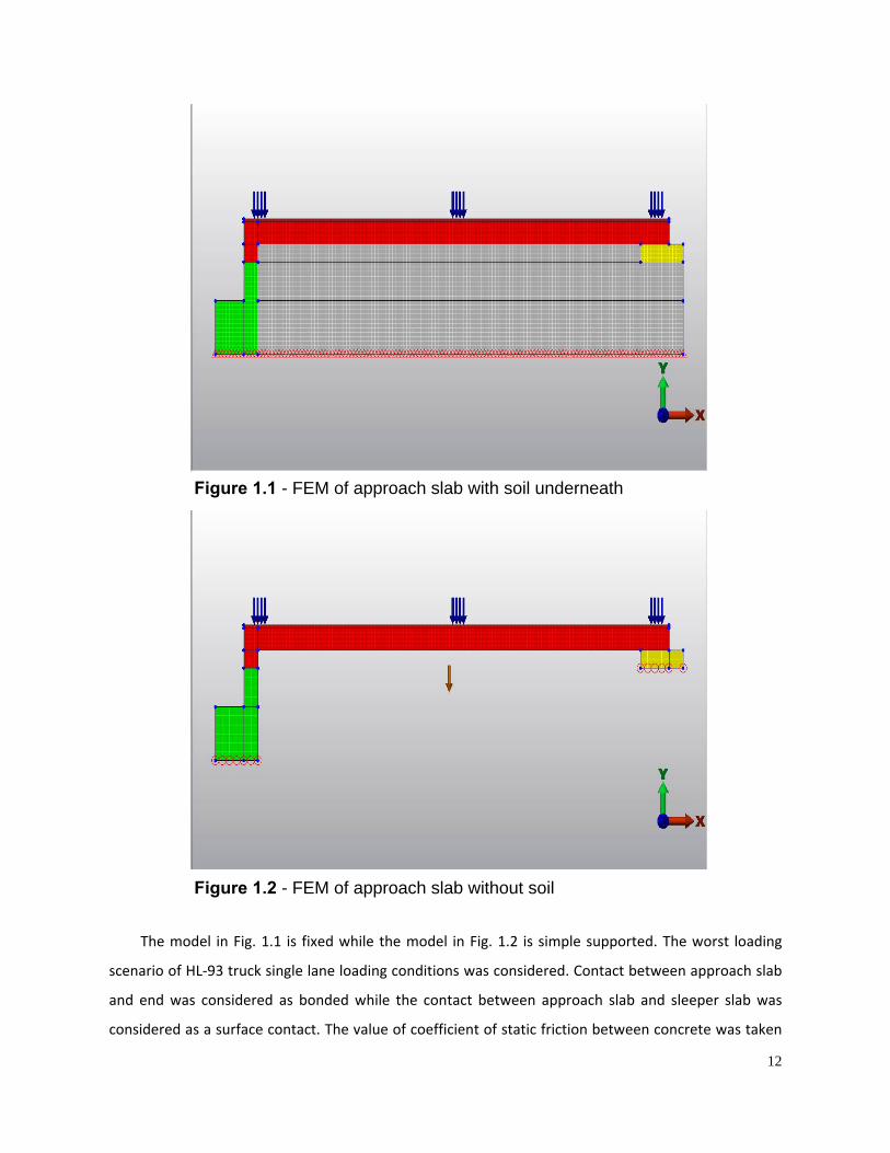
Finite element analysis of Ohio approach  slab was performed by building 2 different models of 

approach  slab  in ALGOR. First model was built  considering  the  soil  is underneath  the approach  slab 

while the second model was built considering all the soil has moved out underneath the approach slab, 

as shown in Fig. 1.1 and 1.2, respectively. The geometric parameters for both approach slabs were: 

• Length = 30 ft.; Width = 20 ft. 

• Bottom Steel ‐ #10 reinforcing bars @ 6.5 in. c.c. 

• Top Steel and Bent Steel ‐ # 5 reinforcing bars @ 18 in. c.c. 

• Vertical Steel ‐ #5 reinforcing bars @ 6 in. c.c.   

State Lmin 

(ft.)

h (in.)

fc' 

(ksi)

As 

(in2/ft)

As’ 

(in2/ft)

d' (in.)

Cc 

(in.)

ΦMn 

(kip*ft/ft)

Mu 

(kip*ft/ft)

AZ 15 12 3 1.053 0.133 2.5 3 37.57 9.77

FL* 30 12 4.5 1.053 0.310 2.5 4 31.05 80.03

IN 20 10 4 0.630 0.203 2.5 2 19.14 30.16

KY 25 17 3.5 1.580 0 NP 3 90.10 61.72

MI* 20 12 4.5 0.895 0.895 3 3 21.87 31.72

OH 30 17 4.5 2.345 0.207 3 3 129.81 90.40

PA 25 16 3.5 1.693 0.310 2.5 3 85.22 60.50

Results on Bridges without bumps Bridges with bumps

COL 30 2578

COL 30 2667

COL 30 11 2L

COL 30 2670

COL 30 3182

Liquid Limit 34.1 21.5 24.9 33.6 32.2 Plastic Limit 24.5 25.5 21.9 30.7 38.4

Plasticity Index

9.6 NP 3.4 2.9 NP

Soil Classifi-cation

A-2-4 (0) A-3 (0) A-1-b (0) A-1-b (0) A-3 (0)

Table 1.1 – AASHTO Soil Classification of different soil samples

Table 1.2 - Approach Slab Designs in different state DOTs

* denotes that applied moment is more than internal moment capacity; NP means Not Provided

12

The model  in Fig. 1.1  is  fixed while  the model  in Fig. 1.2  is simple supported. The worst  loading 

scenario of HL‐93 truck single lane loading conditions was considered. Contact between approach slab 

and end was  considered  as bonded while  the  contact between  approach  slab and  sleeper  slab was 

considered as a surface contact. The value of coefficient of static friction between concrete was taken 

Figure 1.1 - FEM of approach slab with soil underneath

Figure 1.2 - FEM of approach slab without soil

13

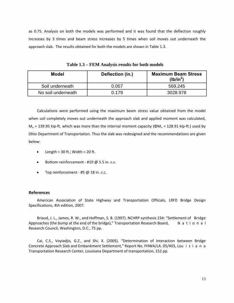
as  0.75. Analysis  on  both  the models was  performed  and  it was  found  that  the  deflection  roughly 

increases  by  3  times  and  beam  stress  increases  by  5  times when  soil moves  out  underneath  the 

approach slab.  The results obtained for both the models are shown in Table 1.3.  

 

Calculations were  performed  using  the maximum  beam  stress  value  obtained  from  the model 

when soil completely moves out underneath  the approach slab and applied moment was calculated, 

Mu = 139.95 kip‐ft. which was more than the internal moment capacity (ΦMn = 128.91 kip‐ft.) used by 

Ohio Department of Transportation. Thus the slab was redesigned and the recommendations are given 

below: 

• Length = 30 ft.; Width = 20 ft. 

• Bottom reinforcement ‐ #10 @ 5.5 in. c.c. 

• Top reinforcement ‐ #5 @ 18 in. c.c. 

 

References 

American  Association  of  State  Highway  and  Transportation  Officials,  LRFD  Bridge  Design Specifications, 4th edition, 2007. 

 

Briaud, J. L., James, R. W., and Hoffman, S. B. (1997). NCHRP synthesis 234: “Settlement of   Bridge Approaches (the bump at the end of the bridge),” Transportation Research Board,   N a t i o n a l Research Council, Washington, D.C., 75 pp. 

 

Cai,  C.S.,  Voyiadjis,  G.Z.,  and  Shi,  X.  (2005).  “Determination  of  Interaction  between  Bridge Concrete Approach Slab and Embankment Settlement,” Report No. FHWA/LA. 05/403, Lou  i s i a n a Transportation Research Center, Louisiana Department of transportation, 152 pp. 

    

Model Deflection (in.) Maximum Beam Stress (lb/in2)

Soil underneath 0.057 569.245

No soil underneath 0.179 3028.978

Table 1.3 – FEM Analysis results for both models

14

Safety Evaluation of Diamond‐grade vs. High‐intensity Retroreflective Sheeting on Work Zone Drums 

Stephen G. Busam Graduate Research Assistant, Department of Civil Engineering, Ohio University  PROJECT SUMMARY 

Each year more than 700 fatalities occur nationally due to vehicular accidents within work zones. 

New developments and technologies have paved the way for the creation of diamond‐grade sheeting, 

a  new, more  retroreflective  sheeting.  Research  has  shown  that  diamond‐grade  sheeting  is  6  to  14 

times brighter  then engineering‐grade  sheeting and  is already widely  required  for use on work zone 

signs. However, the diamond‐grade sheeting is not widely required for use on channelizing drums due 

to  the  increased  cost  and  concern  that  the  increased  retroreflectivity  of  the  sheeting may  actually 

decrease the safety of the work zone when used on closely spaced construction drums. A comparative 

parallel study was conducted to compare the safety impacts of the diamond‐grade sheeting with high‐

intensity sheeting, the current MUTCD standard. Driver behavior within the work zone was analyzed in 

terms of  lane placement and traveled speed with respect to the posted speed  limit. These data were 

collected  and  analyzed  to  determine  the  extent  to which  the  behaviors  differed  between  the  two 

traffic  control  treatments.  A  current  state  of  practices  survey  was  also  distributed  to  each  state 

department of transportation to determine the extent to which diamond‐grade sheeting is being used. 

Approximately 66.7 percent of the state departments of transportation who responded to the survey 

do  not  require  diamond‐grade  sheeting  for  use  in  construction  zones  citing material  cost  as  their 

reasoning. Those states that do require diamond‐grade sheeting for use on drums in their work zones 

listed safety,  improved work zone delineation, and  improved work zone visibility as outweighing  the 

cost of the sheeting. Based on the lane placement and speed deviation data, drivers traveling through 

work zones with diamond‐grade sheeting position their vehicle further away from the work zone and 

abide closer  to  the posted speed  limits when compared  to  those  traveling  through work zones with 

high‐intensity sheeting on the construction drums.  

15

Coupled Thermo‐hydro‐mechanical Model for Pavement Under Frost Action 

Zhen Liu Graduate Student, Case Western Reserve University  

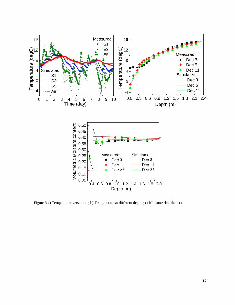
A multiphysical model  is developed  to  analyze  the  coupled hydro‐thermo‐mechanical  fields  for 

porous materials to allow for the behavior of base and subgrade suffering from  inclement climate.  It 

integrates  the  Fourier’s  laws  for  heat  transfer,  Richard’s  equation  for  fluid  transfer,  and  linear 

constitutive  relationship.  In  addition  to  basic  couplings  based  on  thermodynamics,  various  coupled 

parameters were utilized for transferring information between field variables. Additional relationships, 

such as the similarity between drying and freezing processes and Clapeyron equation for  ice balance 

were  incorporated  to  take  into  account  the  effects  of  frost  action.  Numerical  simulations  were 

implemented  in multiphysical  platform  to  solve  the  coupled  nonlinear  partial  differential  equation 

system with  typical  boundary  conditions.  The  high  nonlinear  problem was  turned  out  to  be  solved 

smoothly with stable solutions which cement our understanding of  the phenomena. For application, 

reasonable  simplifications were made  specifically  to  facilitate  the problem  solving process, which  in 

return yield results  lending supports quantitatively to  implementation of the theoretical model. Case 

study on the pavement proves the practical potential of the method and verifies the validation of the 

model as all input base on measured data.  

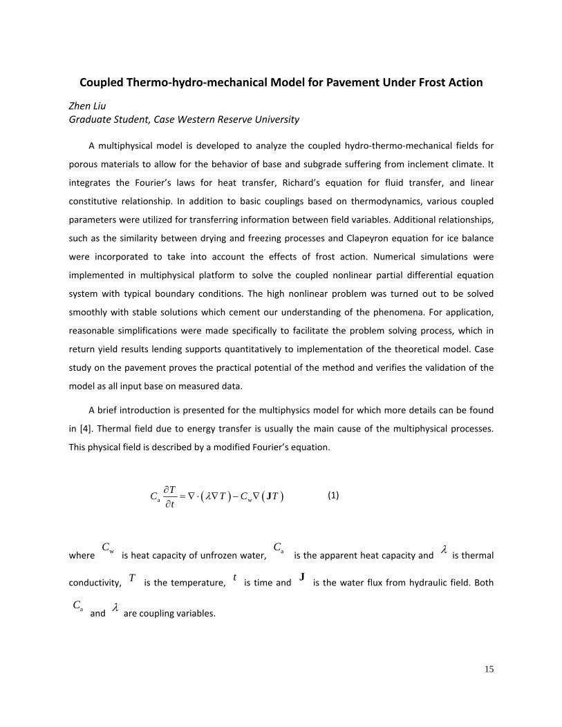
A brief introduction is presented for the multiphysics model for which more details can be found 

in  [4]. Thermal  field due  to energy  transfer  is usually  the main cause of  the multiphysical processes. 

This physical field is described by a modified Fourier’s equation. 

 

        (1) 

 

where   is heat capacity of unfrozen water,    is the apparent heat capacity and  is thermal 

conductivity,    is  the  temperature,    is  time and    is  the water  flux  from hydraulic  field. Both 

 and  are coupling variables.  

wC aC λ

T t J

aC λ

( ) ( )a wTC T C Tt

λ∂= ∇ ⋅ ∇ − ∇

∂J

16

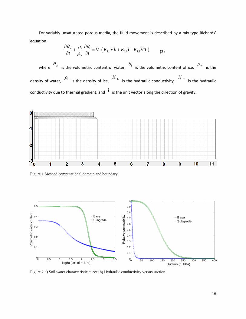
For variably unsaturated porous media, the fluid movement  is described by a mix‐type Richards’ 

equation. 

                                (2) 

where    is the volumetric content of water,    is the volumetric content of  ice,    is the 

density of water,    is the density of  ice,    is the hydraulic conductivity,    is the hydraulic 

conductivity due to thermal gradient, and   is the unit vector along the direction of gravity. 

 

wθ iθ wρ

iρ LhK LTK

i

Figure 1 Meshed computational domain and boundary

0 0.5 1 1.5 2 2.5 3 3.50

0.1

0.2

0.3

0.4

0.5

log(h) (unit of h: kPa)

Vol

umet

ric w

ater

con

tent

BaseSubgrade

0 50 100 150 200 250 300 350 4000

0.1

0.2

0.3

0.4

0.5

0.6

0.7

0.8

0.9

1

Suction (h, kPa)

Rel

ativ

e pe

rmea

bilit

y

BaseSubgrade

Figure 2 a) Soil water characteristic curve; b) Hydraulic conductivity versus suction

( )w i iLh Lh LT

w

K h K K Tt t

θ ρ θρ

∂ ∂+ = ∇ ⋅ ∇ + + ∇

∂ ∂i

17

0 1 2 3 4 5 6 7 8 9 10

-4

0

4

8

12

16

Simulated: S1 S3 S5 AirT

Te

mpe

ratu

re (d

egC

)

Time (day)

Measured: S1 S3 S5

0.0 0.3 0.6 0.9 1.2 1.5 1.8 2.1 2.4-4

0

4

8

12

16

Simulated: Dec 3 Dec 5 Dec 11

Tem

pera

ture

(deg

C)

Depth (m)

Measured: Dec 3 Dec 5 Dec 11

0.4 0.6 0.8 1.0 1.2 1.4 1.6 1.8 2.00.050.100.150.200.250.300.350.400.450.50

Simulated: Dec 3 Dec 11 Dec 22

Vol

umet

ric M

oist

ure

cont

ent

Depth (m)

Measured: Dec 3 Dec 11 Dec 22

Figure 3 a) Temperature verse time; b) Temperature at different depths; c) Moisture distribution

18

UT Solar Car Project   

Sean Sheppard, Ethan Matthews, Zachary Linkous, Sherry Ackerman Undergraduate Students, University of Toledo 

 

The University of Toledo Solar Car Team (UTSC) was founded  in 2008 with the goal to build and 

race  a  solar‐powered  car  in  the 2012 American  Solar Challenge.  The event  is  a  cross‐country  time/

endurance race across public highways. The team  is currently designing the university’s first solar car 

with  the  mission  to  educate  students  and  the  greater  community  on  alternative  energy  and  its 

applications,  as well  as  to  build  a  practical  solar  car  that  could  have  real world  applications  upon 

further technological advances. The team has a strong desire to innovate and use local technology and 

resources. Since Toledo is moving to redefine itself as America’s Solar City, the UTSCT desires to build a 

car that stands out and represents the alternative energy community  in Northwest Ohio. The team  is 

currently designing its car and actively seeking sponsors. The final product is going to feature new and 

original technology including a custom built energy efficient Hub Motor as well as other unique energy‐

saving technologies. The organization  is very excited to be part of the alternative energy solution and 

to help raise community awareness about solar technology. 

The University of Toledo Solar Car Team (UTSC) was originally founded in 2008 but due to most of 

the team graduating, did not get off the ground until the summer of 2010. With momentum building, 

the team has chosen to focus its efforts on five main goals:  

Education 

Innovation 

Promoting local technology 

Design, build and race a practical solar car 

Compete in the 2012 American Solar Car Challenge 

 

We  strive  to  educate  students  and  the  local  community  about  various  alternative  energy 

technologies.   The  innovation refers  to  taking  those previously developed  technologies and  trying  to 

use  them  in different applications. We also aim  to not only promote our University but also  to help 

Toledo with its goal of trying to reinvent itself as the Solar City.  

19

As for practicality, one way we wish to be practical is economically. We are estimating the price of 

our  car  to  be  somewhere  between  $60,000‐  $80,000 whereas  other  solar  cars  could  be  anywhere 

between $1 million and $10 million. We plan  to keep expenses down partially by building our own 

motor and not using space grade solar cells. The other ways we will keep our expenses down are by the 

different technologies that we are planning on incorporating into our car which will maximize the car’s 

energy usage. 

Once  every  two  years,  Universities  all  over  the  country  have  competed  in  this  “rayce”  (the 

American  Solar Challenge)  to  see who  can  finish  first  in  this  cross‐country  event  ranging  anywhere 

between 1200‐1600 miles across public highways. The previous race went from Broken Arrow, OK to 

Naperville,  IL.  The next  race will occur  in  the  summer of 2012 but  the  specifics have not  yet been 

announced.  

Because  the group was  recently  founded and has no previous models,  the  team has chosen  to 

investigate all facets of the car to try and gain an advantage against the more established teams.  Some 

of the mechanical aspects that the team is trying to be innovative with include: an in‐wheel hub motor 

design, possibly airless tires, and also the body design of the car. Most cars in the Solar Car Challenge 

look very similar to flat pancakes on wheels. Our body design looks more like a tear drop or wing shape 

to increase aerodynamics and so the car resembles more of a “normal” car shape. All other mechanical 

aspects of  the car will be consist of parts  that can either be easily be  fabricated or bought  so as  to 

minimize the complexity of not only building, but also working on the car.  

For the upcoming race, the team has chosen to spend a lot of time innovating the electrical side of 

the car, trying to make it as unique as possible. This past semester, the electrical team has been busy at 

work researching and doing simulations to figure out the optimum design for the in‐wheel hub motor 

design. The other electrical aspects of  the car  that students have been working with are  the battery 

management  system  and  a  solar  golf  cart  project.  This  battery management  system  uses  a  pulse 

controller, which will maximize the efficiency of energy transfer during charging and discharging of the 

batteries. 

Another process of electrical designing  is  the hub motor.  It  is based on  the unique  technology 

invented  by  Flynn Motor  Technologies,  but  our  system  has  the  unique  ability  to  recover  inductive 

energy while the motor  is  in operation, and this  is  in addition to the standard regenerative breaking 

technology. These technologies will integrated to give our car both performance, and energy efficiency 

advantages. 

20

Since our car and the technology involved is a reflection of the innovations taking place at UT, we 

are working on  various  innovative electronics  and battery  systems  to  allow us  to  leverage  some of 

these amorphous solar technologies  in our system design to show how a solar car could someday be 

developed into a practical technology for everyday use.  

 

For further information please contact: 

James Price 

University of Toledo Solar Car Team President 

University of Toledo 

2801 W. Bancroft , MS 310 

  Toledo , OH 43606 

(419) 701‐4404 

  utoledosolarcar@gmail.com Priceja6@gmail.com

21

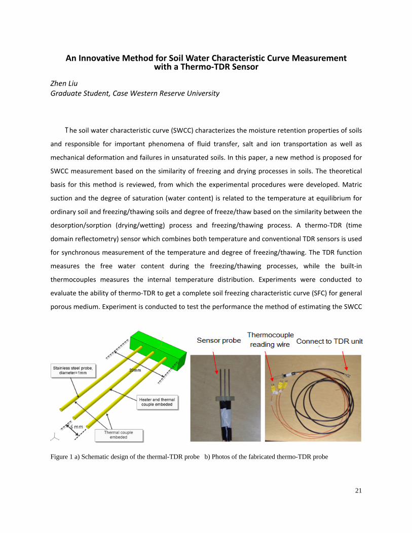
An Innovative Method for Soil Water Characteristic Curve Measurement                             with a Thermo‐TDR Sensor 

Zhen Liu Graduate Student, Case Western Reserve University  

The soil water characteristic curve (SWCC) characterizes the moisture retention properties of soils 

and  responsible  for  important  phenomena  of  fluid  transfer,  salt  and  ion  transportation  as well  as 

mechanical deformation and failures in unsaturated soils. In this paper, a new method is proposed for 

SWCC measurement based on the similarity of freezing and drying processes  in soils. The theoretical 

basis  for  this method  is  reviewed,  from which  the experimental procedures were developed. Matric 

suction and the degree of saturation (water content)  is related to the temperature at equilibrium for 

ordinary soil and freezing/thawing soils and degree of freeze/thaw based on the similarity between the 

desorption/sorption  (drying/wetting)  process  and  freezing/thawing  process.  A  thermo‐TDR  (time 

domain reflectometry) sensor which combines both temperature and conventional TDR sensors is used 

for synchronous measurement of the temperature and degree of freezing/thawing. The TDR function 

measures  the  free  water  content  during  the  freezing/thawing  processes,  while  the  built‐in 

thermocouples  measures  the  internal  temperature  distribution.  Experiments  were  conducted  to 

evaluate the ability of thermo‐TDR to get a complete soil freezing characteristic curve (SFC) for general 

porous medium. Experiment is conducted to test the performance the method of estimating the SWCC 

Figure 1 a) Schematic design of the thermal-TDR probe b) Photos of the fabricated thermo-TDR probe

22

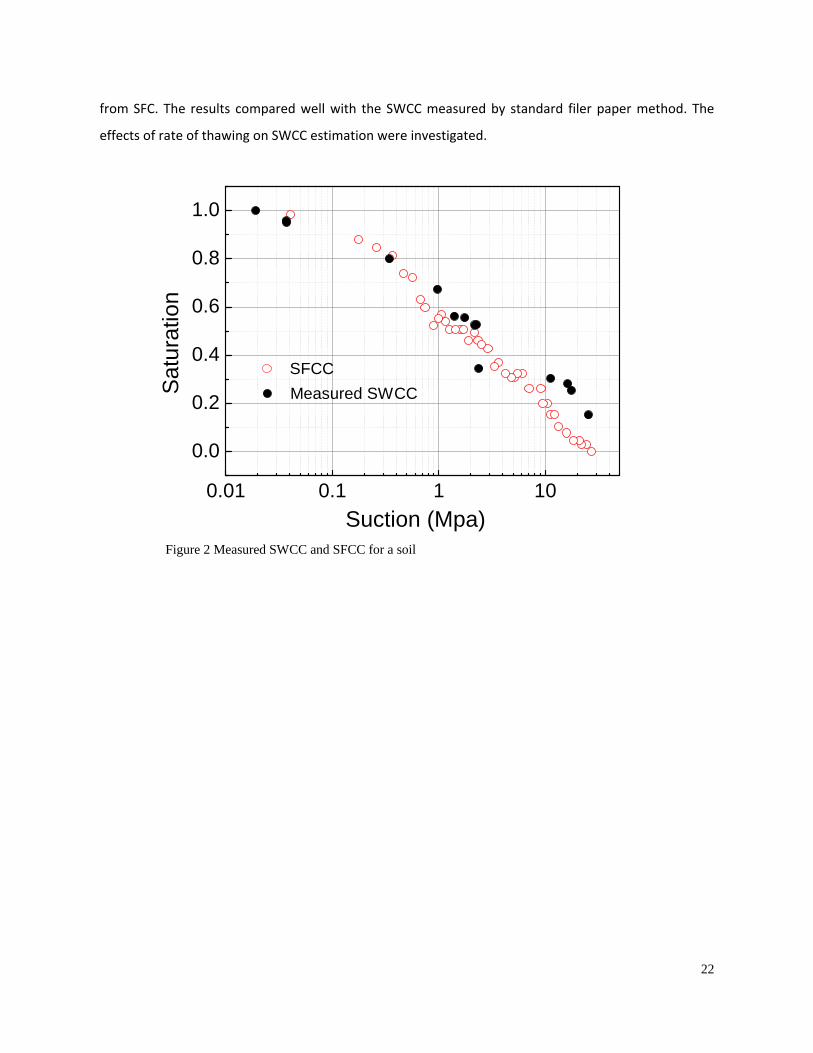
Figure 2 Measured SWCC and SFCC for a soil

0.01 0.1 1 10

0.0

0.2

0.4

0.6

0.8

1.0

Sat

urat

ion

SFCC

Suction (Mpa)

Measured SWCC

from SFC. The  results compared well with  the SWCC measured by standard  filer paper method. The 

effects of rate of thawing on SWCC estimation were investigated.   

 

23

Laboratory Experiments on the Variation of Hydraulic Roughness in Partially Filled Culverts for Fish Passage Design 

Jay Prakash Devkota Graduate Student, Youngstown State University  Introduction 

Culverts  are  hydraulic  conduits  that  serve  to  convey water  from one  side  of  a highway  to  the 

other. Culverts are generally a single run of pipe or box section that  is open at both ends. In general, 

culverts  serve  two main purposes,  first  and narrowest  scope  is  that  they provide  a  conveyance  for 

surface water and storm water under a  roadbed or  railroad grade, and secondly  they allow  fish and 

wildlife passage under the transportation route  

Previously  Transportation was  considered  only  for  connecting  people.  But with  the  increasing 

knowledge of negative effects in aquatic ecology, Engineers are now requested to design culverts that 

minimize the barriers for fish passage. The more common culvert materials used  in the state of Ohio 

are HDPE and steel (smooth and corrugated).  

All of the fish passage design methods seek to allow passage when fish are believed to be moving 

in  the  natural  stream  system.  Excessive  inlet  velocity  and  inadequate  water  depth  may  restrict 

successful passage of fish through the culvert.  

Water  velocity within  a  culvert  is  a  function  of  cross  sectional  area,  slope,  roughness  and  the 

design  discharge.  Among  all  factors,  culvert  roughness  is  the most  readily manipulated  factor  that 

influences velocity.  If  the velocity  in a  culvert exceeds a certain  level,  it may act as a barrier  to  fish 

attempting to ascend upstream. Flow velocities can be reduced by  increasing culvert size, roughness, 

burial depth, and by reducing culvert slope. Reduced velocities in the hydraulic boundary layer on the 

edge of the culvert barrels are seldom adequate for upstream fish passage through the  length of the 

culvert.  

Goal of my proposed Research 

The results of this project are expected to allow engineers to better evaluate existing culverts 

and to better design future culverts for fish passage.  

Literature Review 

My  project  builds  on  a  literature  review  of  Steve  Mangin’s  thesis  on  “Reducing  the  Error 

Associated with Manning's Roughness  in Culvert Design  for  Improved  Fish  Passage”. He  found  that 

24

velocities  in culvert barrels will usually be greater at the medium flow condition than at  low flow  i.e. 

roughness is partial filled pipe/culvert is usually higher than full flow condition.  

Based on the research questions that emerged as a result of Mangin’s study I will be investigating 

data at depths below 20%.  

Methodology:  

The major hydraulic criteria influencing fish passage are: flow rates during migration periods: and 

material  roughness,  depth,  diameter  and  slope  of  the  culvert.  So  the  data  collection  consists  of 

measurement of discharge and depth  for different  values of diameter and  slope with  two different 

material types.  

Manning’s Equation:  

Manning’s Equation is an empirical equation applied to uniform flow in open channels.  

V = Cn/n * R2/3 * S1/2  

Laboratory set up:  

The laboratory model will be a flume of 4ft * 2ft * 60ft (w*h*l) with culvert. The culverts will be in 

this flume. 

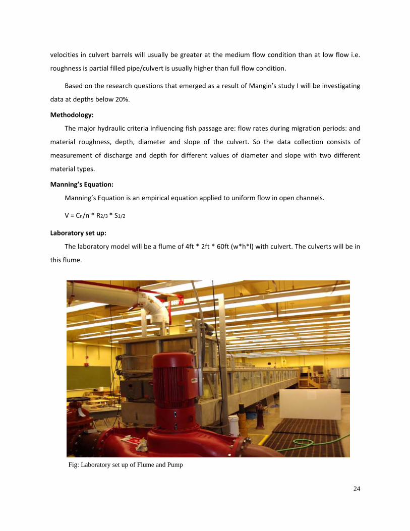
 Fig: Laboratory set up of Flume and Pump

25

 

Once the culvert is placed inside the flume and with the help of a pump the water is pumped into 

the flume at a rate of up to 12 cuft/sec. The pump has overall 38 turns. The flume has a tilting bed so 

that we can change the slope of the flume/ culvert by adjusting from the bed of the flume.  

Work Status:  

Accomplished work: 

The week before I arrived, the flume was not functional.  

At this point the flume is one step away from being usable for culvert tests.  

Preparation for setup of the flume and making supports for the culverts.  

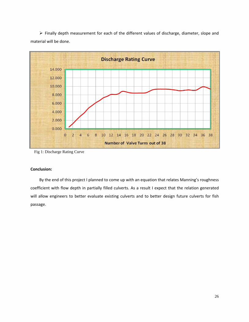
Up to 38 turns of the valve have been completed for the discharge rating curve.  

Remaining work:  

Putting the culverts in the flume. This will be done by the pulley system hanged in the ceiling of 

       the lab.  

Making provisions for depth measurement in the culvert by making hole or by drilling.  

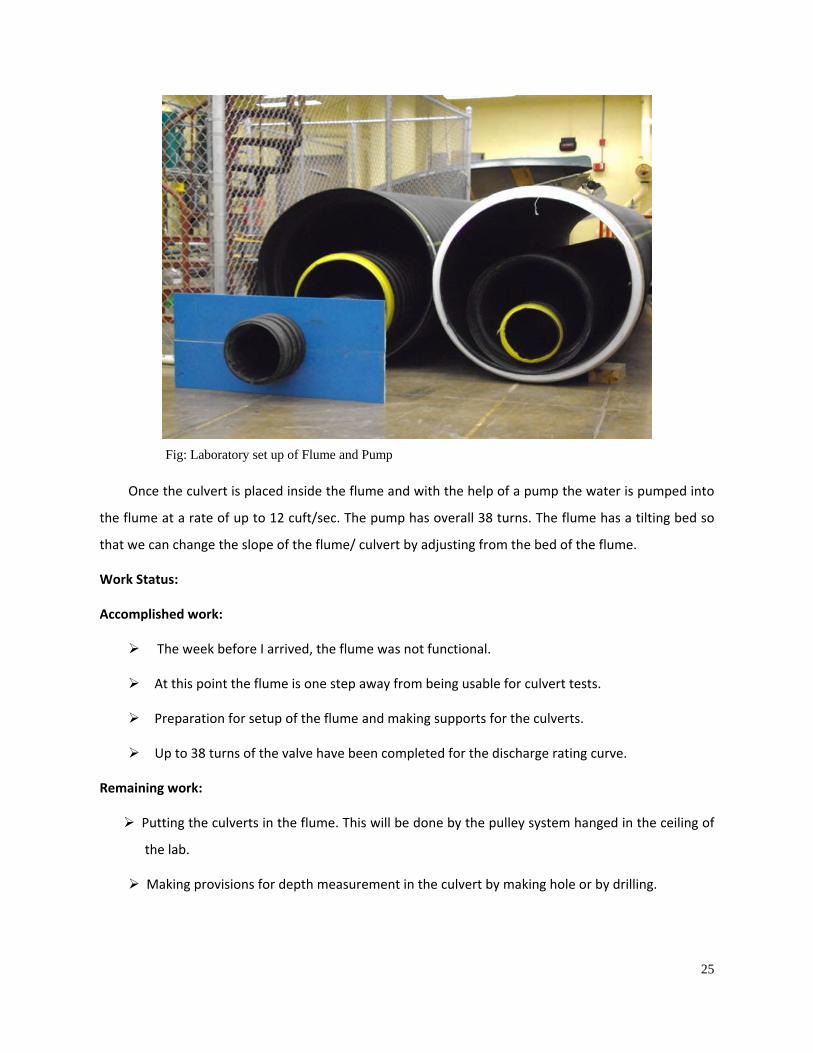
Fig: Laboratory set up of Flume and Pump

26

Finally depth measurement for each of the different values of discharge, diameter, slope and 

material will be done.  

 

Conclusion:  

By the end of this project I planned to come up with an equation that relates Manning’s roughness 

coefficient with flow depth  in partially  filled culverts. As a result  I expect that the relation generated 

will allow engineers  to better evaluate existing  culverts and  to better design  future culverts  for  fish 

passage.  

Fig 1: Discharge Rating Curve

27

Estimating On‐Road Mobile Source Pollution in Ohio 

Ramanitharan Kandiah Assistant Professor, International Center for Water Resources Management, Central State University  André Morton and John Davenport Undergraduate Students, International Center for Water Resources Management, Central State University  Introduction 

Air  pollution  is  significantly  related  to  number  of  health,  environmental  and  also  economical 

effects. Controlling and mitigating air pollution starts with  the understanding of  the pollutants,  their 

sources, and the dispersion mechanisms. Mobile sources that significantly contribute the pollutants to 

the air can be  sub‐classified  into  two groups; On‐Road Mobile Sources  (ORMS) and Nonroad mobile 

sources.  ORMS  which  are  the  concern  of  this  paper  are  comprised  of  the  vehicles  used  for 

transportation  on  roads.  This  category  includes  light‐duty  vehicles,  light‐duty  trucks,  heavy‐duty 

vehicles, and motorcycles. They are mostly operated by variety of fuels, mainly gasoline and diesel, and 

to  a  little  extent  by  natural  gas,  ethanol  and  electricity.  The  On‐Road  Mobile  Source  Pollutants 

(ORMSP)  that  are emitted  from  the ORMS  include   Hydrocarbons, Carbon Monoxide  (CO), nitrogen 

oxides (NOx), particulate matter (PM), air toxics and greenhouse gases. Emitted quantity from an on‐

road  vehicle  depends  on  various  factors;  type  of  the  vehicle,  age  and  operating  condition  of  the 

vehicle, type of the powering fuel, speed the vehicle runs and the distance it travels. Further, the total 

quantity of ORMSAP present in the atmosphere depends on the number of vehicle travels, the time of 

the  day  and  the  surrounding  environment  too.  Given  the  number  of  the  players  involving  in  the 

pollution mechanism, it is difficult to get an accurate estimate for the ORMSAP in the atmosphere. 

This paper presents a methodology that provides preliminary estimates for the ORMSPs released 

in each counties of a  region. The methodology  is demonstrated with a case study  in  the counties of 

Ohio. 

Methodology 

Total Emission for Segment (TES) is defined as the metrics of all individual ORMSP emissions for a 

road segment. It  is computed as the product of Vehicle Miles Traveled (VMT) and actual emissions of 

ORMSPs per mile.  Total emission of each ORMSP in the interested area (such as a county) is computed 

28

by adding the TES metric of the particular ORMSP within that area. The emission intensity, defined as 

emitted ORMSP quantity per area is calculated by dividing the total emission by the area. The findings 

are visualized on ArcGIS. 

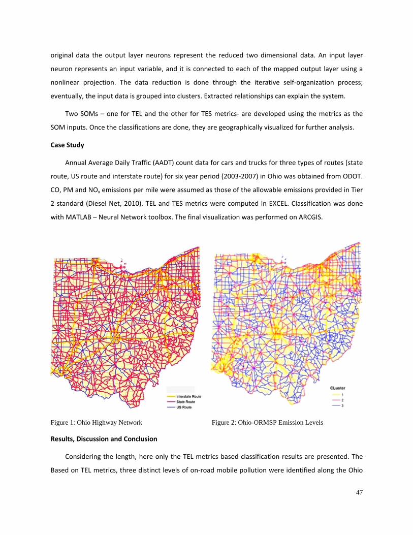
Case Study    

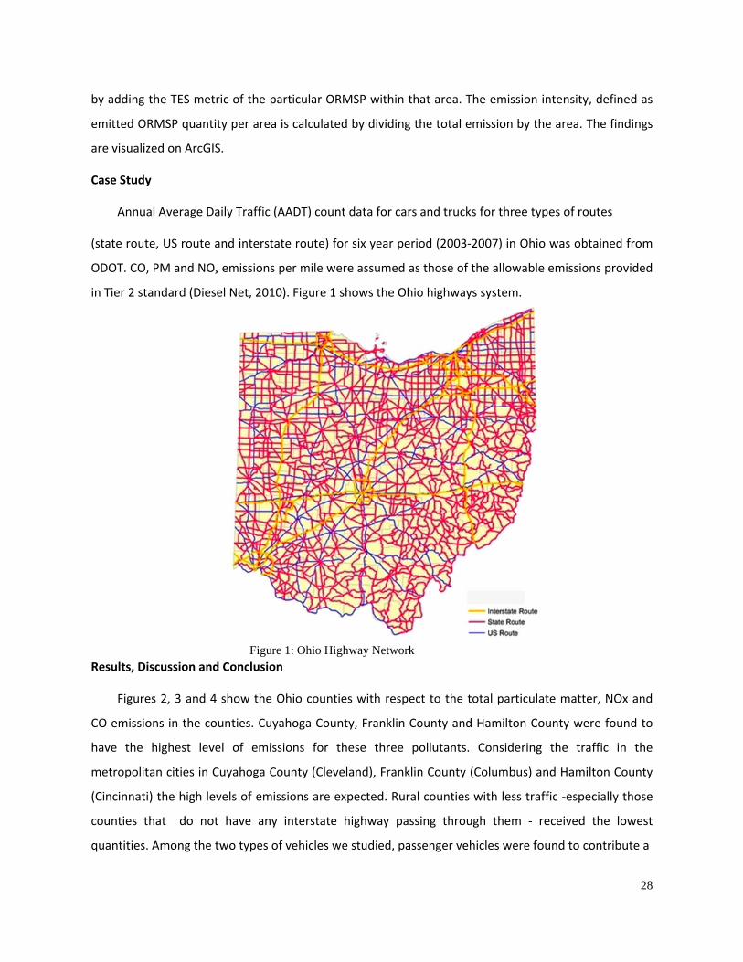
  Annual Average Daily Traffic (AADT) count data for cars and trucks for three types of routes  

(state route, US route and interstate route) for six year period (2003‐2007) in Ohio was obtained from 

ODOT. CO, PM and NOx emissions per mile were assumed as those of the allowable emissions provided 

in Tier 2 standard (Diesel Net, 2010). Figure 1 shows the Ohio highways system. 

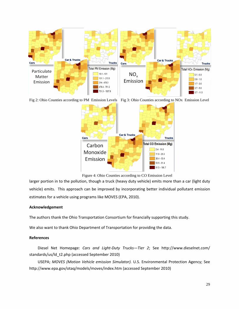
Results, Discussion and Conclusion 

Figures 2, 3 and 4 show the Ohio counties with respect to the total particulate matter, NOx and 

CO emissions  in the counties. Cuyahoga County, Franklin County and Hamilton County were found to 

have  the  highest  level  of  emissions  for  these  three  pollutants.  Considering  the  traffic  in  the 

metropolitan cities in Cuyahoga County (Cleveland), Franklin County (Columbus) and Hamilton County 

(Cincinnati) the high levels of emissions are expected. Rural counties with less traffic ‐especially those 

counties  that    do  not  have  any  interstate  highway  passing  through  them  ‐  received  the  lowest 

quantities. Among the two types of vehicles we studied, passenger vehicles were found to contribute a  

Figure 1: Ohio Highway Network

29

larger portion in to the pollution, though a truck (heavy duty vehicle) emits more than a car (light duty 

vehicle) emits.   This approach can be  improved by  incorporating better  individual pollutant emission 

estimates for a vehicle using programs like MOVES (EPA, 2010). 

Acknowledgement 

The authors thank the Ohio Transportation Consortium for financially supporting this study.  

We also want to thank Ohio Department of Transportation for providing the data. 

References 

Diesel  Net  Homepage:  Cars  and  Light‐Duty  Trucks—Tier  2;  See  http://www.dieselnet.com/

standards/us/ld_t2.php (accessed September 2010) 

USEPA; MOVES  (Motion Vehicle emission Simulator). U.S. Environmental Protection Agency; See 

http://www.epa.gov/otaq/models/moves/index.htm (accessed September 2010) 

Fig 2: Ohio Counties according to PM Emission Levels

Figure 4: Ohio Counties according to CO Emission Level

Fig 3: Ohio Counties according to NOx Emission Level

30

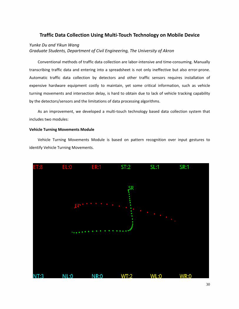
Traffic Data Collection Using Multi‐Touch Technology on Mobile Device 

Yunke Du and Yikun Wang  Graduate Students, Department of Civil Engineering, The University of Akron  

Conventional methods of traffic data collection are labor‐intensive and time‐consuming. Manually 

transcribing  traffic data and entering  into a spreadsheet  is not only  ineffective but also error‐prone. 

Automatic  traffic  data  collection  by  detectors  and  other  traffic  sensors  requires  installation  of 

expensive  hardware  equipment  costly  to  maintain,  yet  some  critical  information,  such  as  vehicle 

turning movements and  intersection delay,  is hard to obtain due to  lack of vehicle tracking capability 

by the detectors/sensors and the limitations of data processing algorithms.  

As an  improvement, we developed a multi‐touch  technology based data  collection  system  that 

includes two modules: 

Vehicle Turning Movements Module 

Vehicle  Turning  Movements  Module  is  based  on  pattern  recognition  over  input  gestures  to 

identify Vehicle Turning Movements. 

31

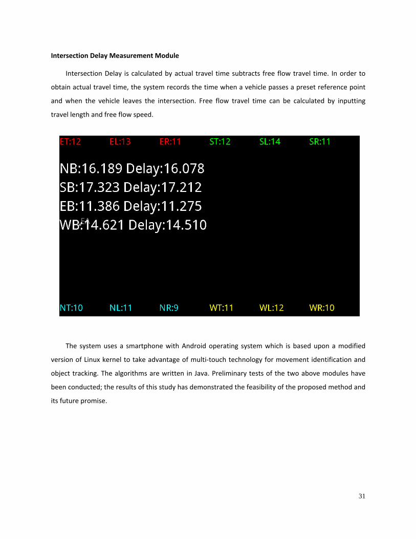
Intersection Delay Measurement Module  

Intersection Delay  is calculated by actual  travel  time subtracts  free  flow  travel  time.  In order  to 

obtain actual travel time, the system records the time when a vehicle passes a preset reference point 

and when  the  vehicle  leaves  the  intersection.  Free  flow  travel  time  can  be  calculated  by  inputting 

travel length and free flow speed. 

 

The  system uses a  smartphone with Android operating  system which  is based upon a modified 

version of Linux kernel to take advantage of multi‐touch technology for movement  identification and 

object tracking. The algorithms are written  in  Java. Preliminary tests of the two above modules have 

been conducted; the results of this study has demonstrated the feasibility of the proposed method and 

its future promise. 

 

32

Effects of Left‐Side Ramps on Crash Frequency on Urban Freeway Segments 

Aline R. Aylo and Worku Y. Mergia  Graduate Students, University of Dayton  

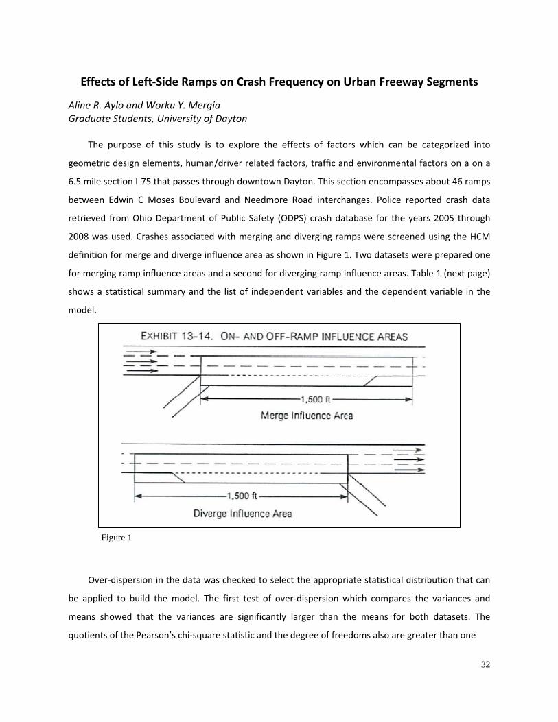
The  purpose  of  this  study  is  to  explore  the  effects  of  factors  which  can  be  categorized  into 

geometric design elements, human/driver related factors, traffic and environmental factors on a on a 

6.5 mile section I‐75 that passes through downtown Dayton. This section encompasses about 46 ramps 

between  Edwin  C Moses  Boulevard  and  Needmore  Road  interchanges.  Police  reported  crash  data 

retrieved  from Ohio Department of Public Safety  (ODPS) crash database  for  the years 2005  through 

2008 was used. Crashes associated with merging and diverging ramps were screened using the HCM 

definition for merge and diverge influence area as shown in Figure 1. Two datasets were prepared one 

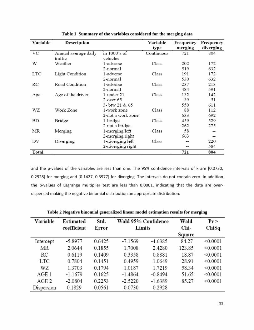
for merging ramp influence areas and a second for diverging ramp influence areas. Table 1 (next page)  

shows a statistical summary and  the  list of  independent variables and  the dependent variable  in  the 

model. 

 

Over‐dispersion in the data was checked to select the appropriate statistical distribution that can 

be  applied  to  build  the model.  The  first  test  of  over‐dispersion which  compares  the  variances  and 

means  showed  that  the  variances  are  significantly  larger  than  the  means  for  both  datasets.  The 

quotients of the Pearson’s chi‐square statistic and the degree of freedoms also are greater than one  

Figure 1

33

 

and  the p‐values of  the  variables are  less  than one. The 95%  confidence  intervals of  k are  [0.0730, 

0.2928] for merging and [0.1427, 0.3977] for diverging. The  intervals do not contain zero.  In addition 

the  p‐values  of  Lagrange  multiplier  test  are  less  than  0.0001,  indicating  that  the  data  are  over‐

dispersed making the negative binomial distribution an appropriate distribution.  

Table 1 Summary of the variables considered for the merging data

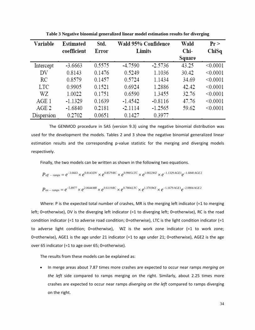
Table 2 Negative binomial generalized linear model estimation results for merging

34

  The GENMOD procedure  in  SAS  (version 9.3) using  the negative binomial distribution was 

used  for the development the models. Tables 2 and 3 show the negative binomial generalized  linear 

estimation  results  and  the  corresponding  p‐value  statistic  for  the  merging  and  diverging  models 

respectively.  

Finally, the two models can be written as shown in the following two equations. 

    

 

 

Where: P is the expected total number of crashes, MR is the merging left indicator (=1 to merging 

left; 0=otherwise), DV  is the diverging  left  indicator (=1 to diverging  left; 0=otherwise), RC  is the road 

condition indicator (=1 to adverse road condition; 0=otherwise), LTC is the light condition indicator (=1 

to  adverse  light  condition;  0=otherwise),    WZ  is  the  work  zone  indicator  (=1  to  work  zone; 

0=otherwise), AGE1  is the age under 21  indicator (=1 to age under 21; 0=otherwise), AGE2  is the age 

over 65 indicator (=1 to age over 65; 0=otherwise). 

The results from these models can be explained as:   

• In merge areas about 7.87 times more crashes are expected to occur near ramps merging on 

the  left  side  compared  to  ramps merging  on  the  right.  Similarly,  about  2.25  times more 

crashes are expected to occur near ramps diverging on the left compared to ramps diverging 

on the right. 

26840.111329.10022.19905.08579.08143.06663.3 AGEAGEWZLTCRCDVrampsoff eeeeeeeP −−−

− ×××××=

Table 3 Negative binomial generalized linear model estimation results for diverging

20804.211679.13703.17804.06119.00644.28977.5 AGEAGEWZLTCRCMRrampson eeeeeeeP −−−

− ×××××=

35

• Expected count of crashes due  to adverse  roadway conditions such as wet pavement, snow 

and ice are found to be 1.84 times more near merging ramps and about 2.36 times more near 

diverging ramps. 

• The  expected  crash  counts  due  to  adverse  light  conditions  such  as  darkness  and  glare  are 

found to be 2.18 times more compared to normal daylight conditions near merging ramps and 

2.70 times more near diverging ramps. 

• The expected  count of  crashes due  to  the presence of  construction work  zone  sections are 

found to be 2.78 times more than sections with no construction near merging ramps and they 

are 3.94 times more near diverging ramps. 

• The expected count of crashes near merging  ramps  is  lesser by a  factor of 0.125  for  senior 

drivers (Age>64) and 0.313 for youth drivers (Age <21) compared to drivers of age range 21‐

64.   

• Similarly,  expected  count  of  crashes  near  diverging  ramps  show  a  decrease  by  a  factor  of 

0.186  for  senior  drivers  (Age>64)  and  0.322  for  youth  drivers  (Age<21)  compared  to  the 

drivers of age range 21‐64. 

 

In  conclusion,  the  prediction  model  developed  here  can  be  used  to  evaluate  the  safety 

performance of left‐side ramps. Left‐side on‐ and off‐ramps are critical traffic safety factors, therefore, 

future designs should avoid  the provision of ramps on  the  left side and safety  improvements should 

consider the safety benefit of replacing them with right‐side ramps.  

 

 

36

Evaluating Traffic Safety Behaviors of College Students 

Sowjanya Ponnada Graduate Studetn, Department of Civil and Environmental Engineering and Engineering Mechanics, University of Dayton   

This  paper  explores  the  traffic  safety  behavior  of  18‐24  yr  old  college  students who  annually 

experience alcohol‐related deaths,  injuries and other health problems.  In addition,  college  student’s 

perceived  causes  related  to  smoking and also not  following  safety measures while driving and  their 

opinions on how to reduce the accidents were included. A sample of 107 full time undergraduate civil 

engineering  students at University of Dayton participated  in  the questionnaire  survey  that assessed 

their demographic characteristics, drinking‐driving, precautionary measures to avoid traffic accidents, 

being involved in crashes as a driver and/or as being involved in crashes when riding in a vehicle driven 

by  someone,  smoking and drinking behavior. The majority of  the  students  reported  that  they never 

drink  alcohol  while.  In  contrast,  the  same  students  reported  that  they  had  been  driven  by  an 

intoxicated driver and almost one‐third of the students reported that they smoke or consume alcohol. 

Age, gender and class,  type of vehicle may play part  in  the evaluation of drinking  ‐ driving behavior, 

smoking‐drinking  and being  involved  in  a  crash. According  to  this  study alcohol‐related,  driving‐risk 

behaviors among college students become worse at the age of 21. There is need to investigate further 

the  relationship  between  the  students  who  consume  alcohol  while  driving  and  riding  with  an 

intoxicated driver, the major reasons to involve traffic crashes. 

37

Dynamic Dilemma Zone at Signalized Intersections: Safety Issue and Solutions 

Zhixia Li Ph.D. Candidate, Advanced Research in Transportation Engineering and Systems Laboratory School of Advanced Structures, College of Engineering and Applied Science, University of Cincinnati  Summary:  

At high speed signalized intersections, the issue of yellow light dilemma is known as a major cause 

of  rear‐end  and  right‐angle  crashes.  This  dilemma  is  typically  characterized  by  a  physical  zone  in 

advance of the intersection, which is termed as dilemma zone (DZ). Drivers in DZ at the onset of yellow 

indication are forced to make a stop/go decision during a very short period. And, an improper decision 

may  lead  them  to  a  potential  rear‐end  or  right‐angle  crash.  Therefore,  it  is  critical  to  accurately 

estimate the exact location of DZ in order to provide necessary DZ protection to drivers. However, one 

apparent barrier in accurately estimating the DZ locations lies in the uncertainty of modeling dynamics 

of  DZ.  Traditional method  for  computing  DZ  uses  constant  contributing  factor  values  that  cannot 

reflect  the  dynamic  features  of DZ.  This  issue  has  been  recognized  for many  years.  In  other word, 

quantitative study of the inherent DZ contributing factors remains a challenge. Lack of effective means 

for gaining the trajectory data over the yellow interval may be a key reason. 

In this research, the author upgraded the software VEVID (Vehicle Video‐Capture Data Collector) 

developed by the author’s advisor. The upgraded VEVID make  it practical to obtain vehicle trajectory 

data  from video,  such as vehicle’s distance  from  stop  line and vehicle’s  speed at every 1/30  second 

during the yellow  interval  including the onset of yellow time. Significantly, this video‐based approach 

has been proved to be an accurate and cost‐effective way for extracting vehicle trajectory data through 

data validation process. Therefore, using this approaching,  it becomes possible to reveal the dynamic 

features of DZ contributing factors and model the extract location of dynamic DZ. The trajectory data 

of  1445  vehicles  are  extracted  in  total  from  46‐hour  high  resolution  videos  at  four  high‐speed 

signalized  intersections  in Ohio using VEVID. The  statistical analyses of  the obtained  trajectory data 

quantitatively  disclose  the  dynamic  natures  of major  DZ  contributing  factors,  such  as  the  driver’s 

minimum perception‐reaction time  (PRT), the vehicle’s maximum acceleration rate, and the vehicle’s 

maximum deceleration rate. The results indicate that (1) the minimum PRT is greatly influenced by the 

vehicle’s speed and can be mathematically modeled as a function of the speed by the Inverse model. 

i.e.,  the minimum PRT decreases as  the vehicle’s  speed  increases  (See Figure 1);    (2)  the maximum 

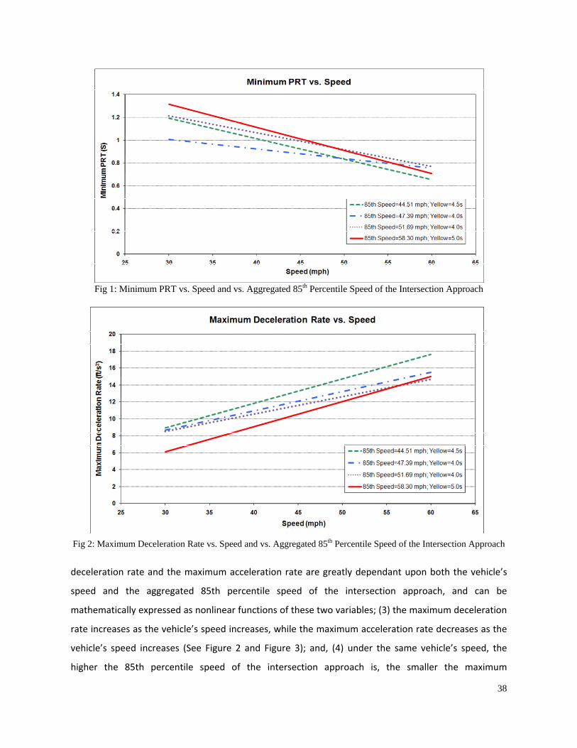
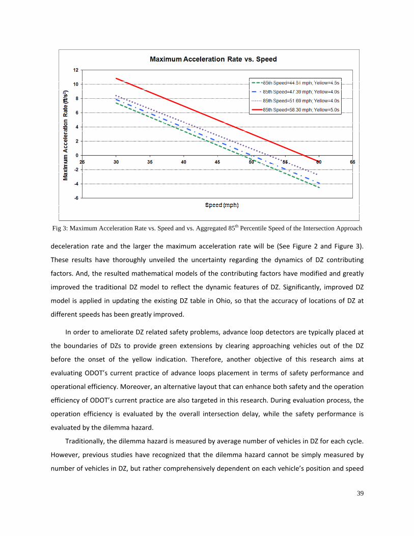
38

deceleration rate and  the maximum acceleration rate are greatly dependant upon both the vehicle’s 

speed  and  the  aggregated  85th  percentile  speed  of  the  intersection  approach,  and  can  be 

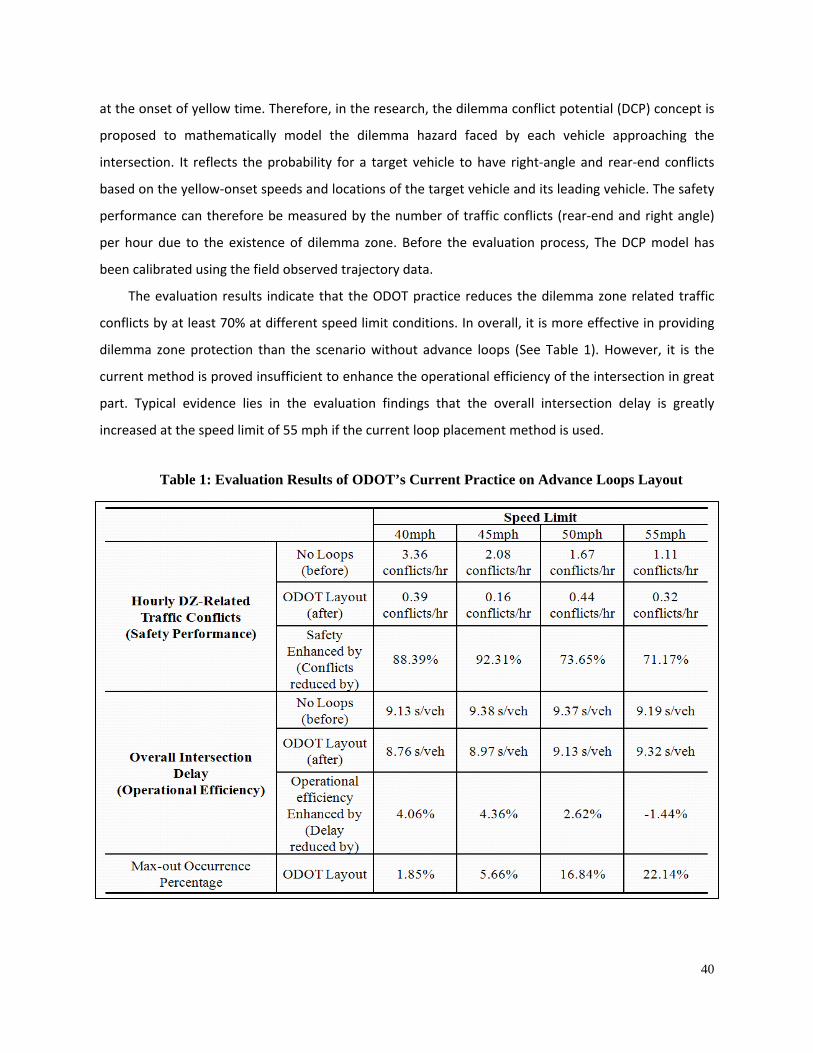
mathematically expressed as nonlinear functions of these two variables; (3) the maximum deceleration 

rate increases as the vehicle’s speed increases, while the maximum acceleration rate decreases as the 

vehicle’s  speed  increases  (See  Figure 2  and  Figure 3);  and,  (4) under  the  same  vehicle’s  speed,  the 

higher  the  85th  percentile  speed  of  the  intersection  approach  is,  the  smaller  the  maximum 

Fig 2: Maximum Deceleration Rate vs. Speed and vs. Aggregated 85th Percentile Speed of the Intersection Approach

Fig 1: Minimum PRT vs. Speed and vs. Aggregated 85th Percentile Speed of the Intersection Approach

39

deceleration  rate and  the  larger  the maximum acceleration  rate will be  (See Figure 2 and Figure 3). 

These  results  have  thoroughly  unveiled  the  uncertainty  regarding  the  dynamics  of  DZ  contributing 

factors. And, the resulted mathematical models of the contributing factors have modified and greatly 

improved  the  traditional DZ model  to  reflect  the dynamic  features of DZ. Significantly,  improved DZ 

model  is applied  in updating the existing DZ table  in Ohio, so that the accuracy of  locations of DZ at 

different speeds has been greatly improved.  

In order to ameliorate DZ related safety problems, advance loop detectors are typically placed at 

the  boundaries  of DZs  to  provide  green  extensions  by  clearing  approaching  vehicles  out  of  the DZ 

before  the  onset  of  the  yellow  indication.  Therefore,  another  objective  of  this  research  aims  at 

evaluating ODOT’s current practice of advance  loops placement  in  terms of  safety performance and 

operational efficiency. Moreover, an alternative layout that can enhance both safety and the operation 

efficiency of ODOT’s current practice are also targeted in this research. During evaluation process, the 

operation  efficiency  is  evaluated  by  the  overall  intersection  delay, while  the  safety  performance  is 

evaluated by the dilemma hazard. 

Traditionally, the dilemma hazard is measured by average number of vehicles in DZ for each cycle. 

However, previous  studies have  recognized  that  the dilemma hazard cannot be  simply measured by 

number of vehicles in DZ, but rather comprehensively dependent on each vehicle’s position and speed 

Fig 3: Maximum Acceleration Rate vs. Speed and vs. Aggregated 85th Percentile Speed of the Intersection Approach

40

at the onset of yellow time. Therefore, in the research, the dilemma conflict potential (DCP) concept is 

proposed  to  mathematically  model  the  dilemma  hazard  faced  by  each  vehicle  approaching  the 

intersection.  It  reflects  the probability  for a  target vehicle  to have  right‐angle and  rear‐end conflicts 

based on the yellow‐onset speeds and locations of the target vehicle and its leading vehicle. The safety 

performance can therefore be measured by the number of traffic conflicts (rear‐end and right angle) 

per hour due  to  the existence of dilemma  zone. Before  the evaluation process, The DCP model has 

been calibrated using the field observed trajectory data. 

The evaluation results  indicate  that  the ODOT practice reduces the dilemma zone related traffic 

conflicts by at least 70% at different speed limit conditions. In overall, it is more effective in providing 

dilemma  zone protection  than  the  scenario without advance  loops  (See Table 1). However,  it  is  the 

current method is proved insufficient to enhance the operational efficiency of the intersection in great 

part.  Typical  evidence  lies  in  the  evaluation  findings  that  the  overall  intersection  delay  is  greatly 

increased at the speed limit of 55 mph if the current loop placement method is used. 

Table 1: Evaluation Results of ODOT’s Current Practice on Advance Loops Layout

41

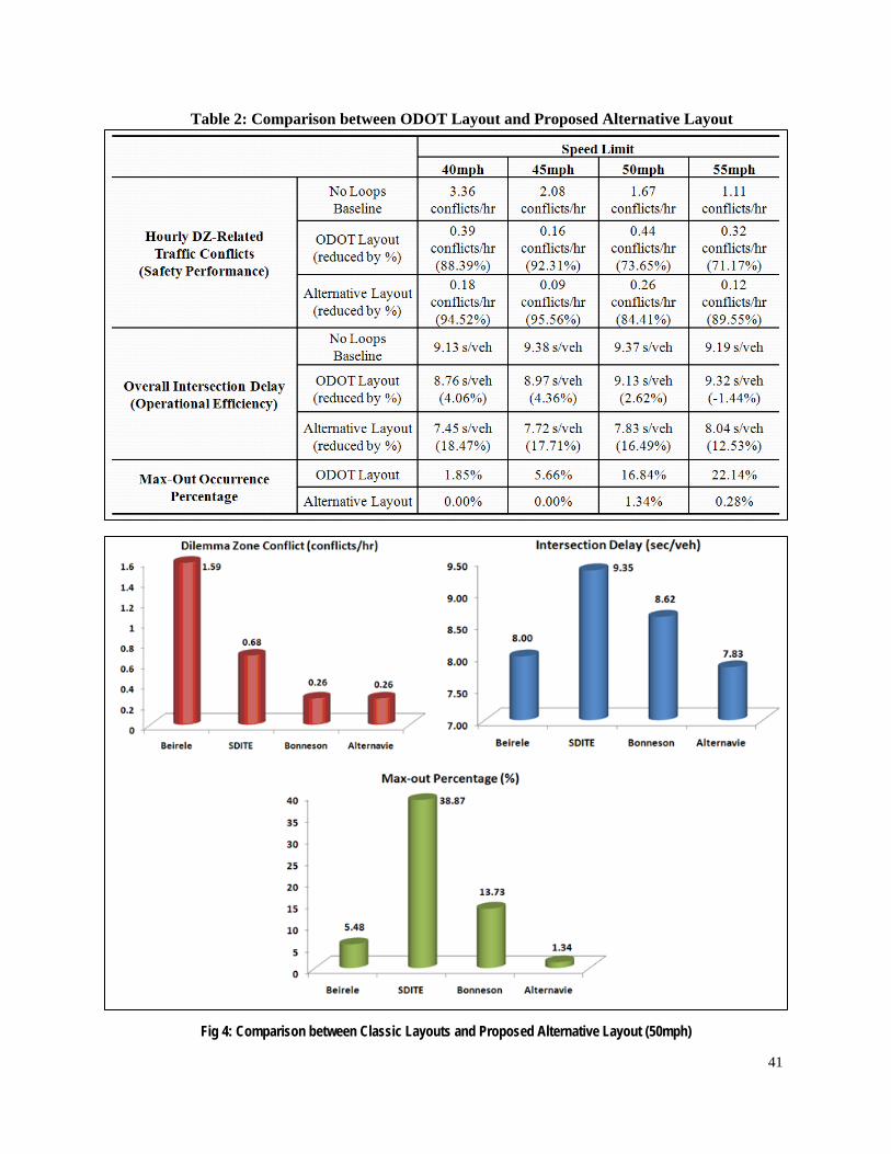
Fig 4: Comparison between Classic Layouts and Proposed Alternative Layout (50mph)

Table 2: Comparison between ODOT Layout and Proposed Alternative Layout

42

The proposed alternative  loops placement outperforms  the ODOT’s current practice  in  terms of 

reducing  the  dilemma  zone  related  traffic  conflicts  by  at  least  84%  under  different  speed  limits. 

Significantly,  it also performs better  in  terms of both operational efficiency and max‐out occurrence 

percentage at all speed  limits, particularly  in  the case of higher speed  limits such as 50 mph and 55 

mph (See Table 2). 

Finally, the proposed alternative loops layout is compared with other classic advance loops layouts 

that  are widely used  in  the US  (See  Figure 4).  The  result has proved  that  the proposed  alternative 

layout  is  superior  to  the  classic  Bonneson,  Beirele,  and  SDITE  layouts  in  terms  of  both  safety 

performance  and  operational  efficiency. Using  50 mph  speed  limit  as  an  example,  the  comparison 

results indicate that the alternative layout is 6 times safer, 1.03 times more efficient, and 4 times less 

likely  to  max  out  as  compared  with  the  Beirele  configuration.  As  compared  with  the  SDITE 

configuration,  it  is 2.6  times safer, 1.2  times more efficient, and 29  times  less  likely  to max out. The 

optimal  layout  is as  safe as  the Bonneson configuration, but  it uses one  less detector. And,  it  is 1.1 

times more  operationally  efficient  and  10  times  less  likely  to max  out  when  compared  with  the 

Bonneson configuration. 

In  summary and  significantly,  the methodology used  in  this  research has potential  to provide a 

theoretical base for other states in the U.S. for updating their existing DZ tables as ones that reflect the 

DZ dynamics, and comprehensively evaluating their existing advance loops layout strategies. 

(This presented study is supported by an OTC grant and an ODOT/FHWA grant, and advised by the author’s advisor, Dr. Heng Wei, Associate Professor at University of Cincinnati. Tel: (513) 556-3781; Email: heng.wei@uc.edu)

43

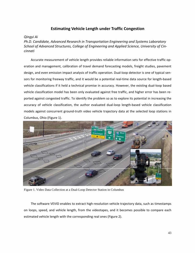
Estimating Vehicle Length under Traffic Congestion 

Qingyi Ai Ph.D. Candidate, Advanced Research in Transportation Engineering and Systems Laboratory School of Advanced Structures, College of Engineering and Applied Science, University of Cin‐cinnati 

Accurate measurement of vehicle length provides reliable information sets for effective traffic op‐

eration and management, calibration of travel demand forecasting models, freight studies, pavement 

design, and even emission impact analysis of traffic operation. Dual‐loop detector is one of typical sen‐

sors for monitoring freeway traffic, and it would be a potential real‐time data source for length‐based 

vehicle classifications if it held a technical promise in accuracy. However, the existing dual‐loop based 

vehicle classification model has been only evaluated against free traffic, and higher error has been re‐

ported against congested traffic. To identify the problem so as to explore its potential in increasing the 

accuracy  of  vehicle  classification,  the  author  evaluated  dual‐loop  length‐based  vehicle  classification 

models against concurrent ground‐truth video vehicle trajectory data at the selected  loop stations  in 

Columbus, Ohio (Figure 1).  

 

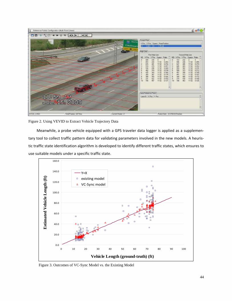
The software VEVID enables to extract high‐resolution vehicle trajectory data, such as timestamps 

on  loops, speed, and vehicle  length,  from  the videotapes, and  it becomes possible  to compare each 

estimated vehicle length with the corresponding real ones (Figure 2).  

Figure 1. Video Data Collection at a Dual-Loop Detector Station in Columbus

44

Meanwhile, a probe vehicle equipped with a GPS traveler data logger is applied as a supplemen‐

tary tool to collect traffic pattern data for validating parameters involved in the new models. A heuris‐

tic traffic state identification algorithm is developed to identify different traffic states, which ensures to 

use suitable models under a specific traffic state.  

 

 

 

Figure 2. Using VEVID to Extract Vehicle Trajectory Data

0.0

20.0

40.0

60.0

80.0

100.0

120.0

140.0

160.0

0 10 20 30 40 50 60 70 80 90 100

Vehicle Length (ground-truth) (ft)

Est

imat

ed V

ehic

le L

engt

h (f

t)

Y=X

existing model

VC‐Sync model

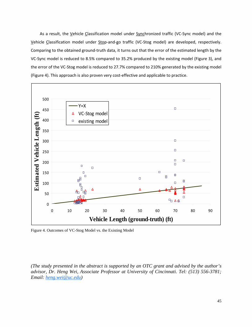
Figure 3. Outcomes of VC-Sync Model vs. the Existing Model

45

As a result, the Vehicle Classification model under Synchronized traffic  (VC‐Sync model) and the 

Vehicle  Classification model  under  Stop‐and‐go  traffic  (VC‐Stog model)  are  developed,  respectively. 

Comparing to the obtained ground‐truth data, it turns out that the error of the estimated length by the 

VC‐Sync model is reduced to 8.5% compared to 35.2% produced by the existing model (Figure 3), and 

the error of the VC‐Stog model is reduced to 27.7% compared to 210% generated by the existing model 

(Figure 4). This approach is also proven very cost‐effective and applicable to practice. 

 

 

(The study presented in the abstract is supported by an OTC grant and advised by the author’s advisor, Dr. Heng Wei, Associate Professor at University of Cincinnati. Tel: (513) 556-3781; Email: heng.wei@uc.edu)

 

0

50

100

150

200

250

300

350

400

450

500

0 10 20 30 40 50 60 70 80 90

Vehicle Length (ground-truth) (ft)

Est

imat

ed V

ehic

le L

engt

h (ft

)

Y=X

VC‐Stog model

existing model

Figure 4. Outcomes of VC-Stog Model vs. the Existing Model

46

Using Datamining in Classifications of Traffic Counting Locations:  

A Case Study in Ohio Ramanitharan Kandiah Assistant Professor, International Center for Water Resources Management, Central State University  John Davenport and André Morton Undergraduate Students, Central State University  Introduction 

On‐Road Mobile Source Pollutants (ORMSP), such as carbon monoxide, nitrogen oxides and some 

hazardous air pollutants are  induced by  the  transportation network. They can  lead  to breathing and 

heart problems, as well as issues with reproduction and even cancer in humans. Hence it is necessary 

to quantify the ORMSP amount and also to identify the hot spots in the routes. The classification and 

the  ranking of  the  road segments can be  looked  into  two ways; according  to  the Total Emission per 

Length of  the  road  (TEL) and  to  the Total Emission per Segment  (TES). The TEL  classification  can be 

used  to  evaluate  the  intensity  of  the  ORMSP  pollution  along  the  transportation  system,  the  TES 

classification can be used to identify the road segments according to their pollutant contribution. 

 This  study explores a methodology  to classify  the  routes with  respect  to  the  level of collective 

ORMSP emission. A case study is presented with Ohio highways traffic data. 

Methodology 

For each road segment, TEL is the metrics of all individual ORMSP emissions per length. Each TEL 

metric  is  computed  as  the product of  actual  emission of  an ORMSP  for  a  vehicle  per mile  and  the 

number  of  the  vehicles  in  the  segment.  TES  for  a  segment  is  the metrics  of  all  individual ORMSP 

emissions  that  is equivalent  to  the product of Vehicle Miles Traveled  (VMT) and actual emissions of 

ORMSPs per mile. Here it is computed by multiplying TEL of the particular segment by the length of the 

segment. Once the TEL metrics and the TES metrics are computed for the transportation network, an 

unsupervised artificial neural network, Self Organizing Map (SOM) is used to classify the sections. 

Self Organizing Maps 

Self  Organizing Map  (SOM)  has  been  extensively  explored  in many  fields  for  the  purposes  of 

classification and pattern recognition (Kohonen, 2001). In SOMs, a competitive learning process is done 

only with  inputs and without desired outputs. While  the  input  layers are high‐dimensional with  the 

47

original data  the output  layer neurons  represent  the  reduced  two dimensional data. An  input  layer 

neuron represents an  input variable, and  it  is connected to each of the mapped output  layer using a 

nonlinear  projection.  The  data  reduction  is  done  through  the  iterative  self‐organization  process; 

eventually, the input data is grouped into clusters. Extracted relationships can explain the system. 

Two SOMs – one  for TEL and  the other  for TES metrics‐ are developed using  the metrics as  the 

SOM inputs. Once the classifications are done, they are geographically visualized for further analysis. 

Case Study    

Annual Average Daily Traffic (AADT) count data for cars and trucks for three types of routes (state 

route, US route and interstate route) for six year period (2003‐2007) in Ohio was obtained from ODOT. 

CO, PM and NOx emissions per mile were assumed as those of the allowable emissions provided in Tier 

2 standard  (Diesel Net, 2010). TEL and TES metrics were computed  in EXCEL. Classification was done 

with MATLAB – Neural Network toolbox. The final visualization was performed on ARCGIS. 

Results, Discussion and Conclusion 

Considering the  length, here only the TEL metrics based classification results are presented. The 

Based on TEL metrics, three distinct levels of on‐road mobile pollution were identified along the Ohio 

Figure 1: Ohio Highway Network Figure 2: Ohio-ORMSP Emission Levels

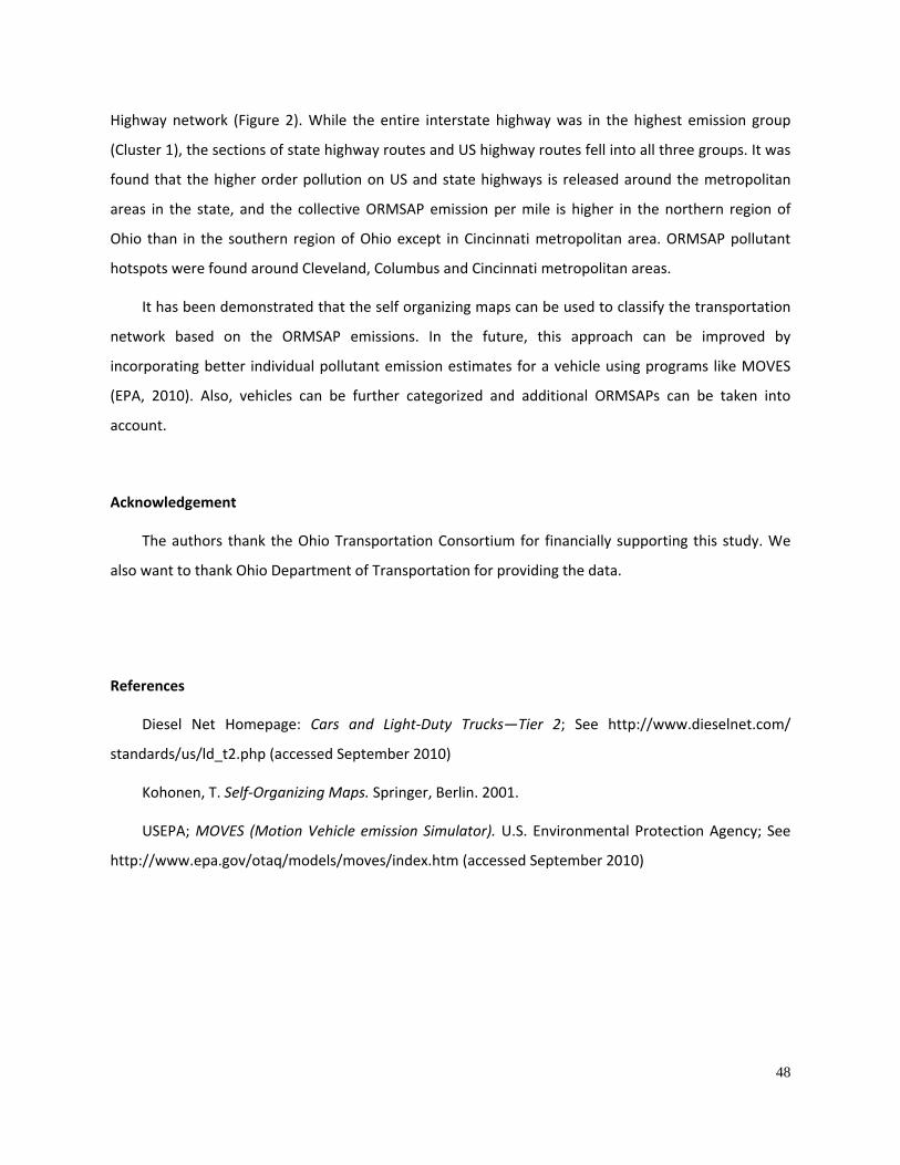
48

Highway network  (Figure 2). While  the entire  interstate highway was  in  the highest emission group 

(Cluster 1), the sections of state highway routes and US highway routes fell into all three groups. It was 

found that the higher order pollution on US and state highways  is released around the metropolitan 

areas  in  the  state, and  the collective ORMSAP emission per mile  is higher  in  the northern  region of 

Ohio  than  in  the southern  region of Ohio except  in Cincinnati metropolitan area. ORMSAP pollutant 

hotspots were found around Cleveland, Columbus and Cincinnati metropolitan areas. 

It has been demonstrated that the self organizing maps can be used to classify the transportation 

network  based  on  the  ORMSAP  emissions.  In  the  future,  this  approach  can  be  improved  by 

incorporating better  individual pollutant emission estimates for a vehicle using programs  like MOVES 

(EPA,  2010).  Also,  vehicles  can  be  further  categorized  and  additional  ORMSAPs  can  be  taken  into 

account. 

 

Acknowledgement 

The authors  thank  the Ohio Transportation Consortium  for  financially supporting  this study. We 

also want to thank Ohio Department of Transportation for providing the data. 

 

 

References 

Diesel  Net  Homepage:  Cars  and  Light‐Duty  Trucks—Tier  2;  See  http://www.dieselnet.com/

standards/us/ld_t2.php (accessed September 2010) 

Kohonen, T. Self‐Organizing Maps. Springer, Berlin. 2001. 

USEPA; MOVES  (Motion Vehicle emission Simulator). U.S. Environmental Protection Agency; See 

http://www.epa.gov/otaq/models/moves/index.htm (accessed September 2010) 

49

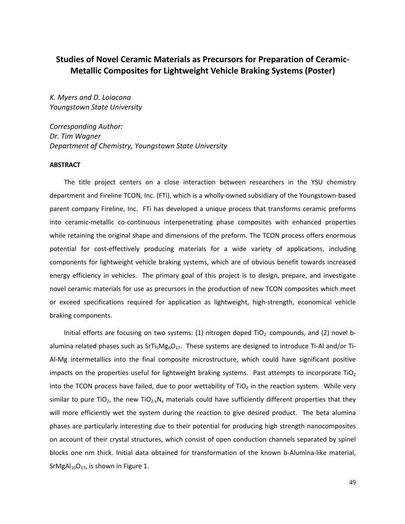
Studies of Novel Ceramic Materials as Precursors for Preparation of Ceramic‐Metallic Composites for Lightweight Vehicle Braking Systems (Poster) 

 K. Myers and D. Loiacona Youngstown State University  Corresponding Author: Dr. Tim Wagner  Department of Chemistry, Youngstown State University  ABSTRACT 

The  title  project  centers  on  a  close  interaction  between  researchers  in  the  YSU  chemistry 

department and Fireline TCON, Inc. (FTi), which is a wholly‐owned subsidiary of the Youngstown‐based 

parent company Fireline,  Inc.   FTi has developed a unique process that  transforms ceramic preforms 

into  ceramic‐metallic  co‐continuous  interpenetrating  phase  composites  with  enhanced  properties 

while retaining the original shape and dimensions of the preform. The TCON process offers enormous 

potential  for  cost‐effectively  producing  materials  for  a  wide  variety  of  applications,  including 

components  for  lightweight vehicle braking systems, which are of obvious benefit towards  increased 

energy efficiency  in vehicles.   The primary goal of  this project  is  to design, prepare, and  investigate 

novel ceramic materials for use as precursors in the production of new TCON composites which meet 

or  exceed  specifications  required  for  application  as  lightweight,  high‐strength,  economical  vehicle 

braking components.    

Initial efforts are focusing on two systems: (1) nitrogen doped TiO2  compounds, and (2) novel b‐

alumina related phases such as SrTi5Mg6O17.  These systems are designed to introduce Ti‐Al and/or Ti‐

Al‐Mg  intermetallics  into  the  final  composite microstructure, which  could  have  significant  positive 

impacts on  the properties useful  for  lightweight braking systems.   Past attempts  to  incorporate TiO2 

into the TCON process have failed, due to poor wettability of TiO2 in the reaction system.  While very 

similar  to pure TiO2,  the new TiO2‐xNx materials could have sufficiently different properties  that  they 

will more efficiently wet  the  system during  the  reaction  to give desired product.   The beta alumina 

phases are particularly  interesting due to their potential for producing high strength nanocomposites 

on account of their crystal structures, which consist of open conduction channels separated by spinel 

blocks one nm  thick.  Initial data obtained  for  transformation of  the  known b‐Alumina‐like material, 

SrMgAl10O17, is shown in Figure 1. 

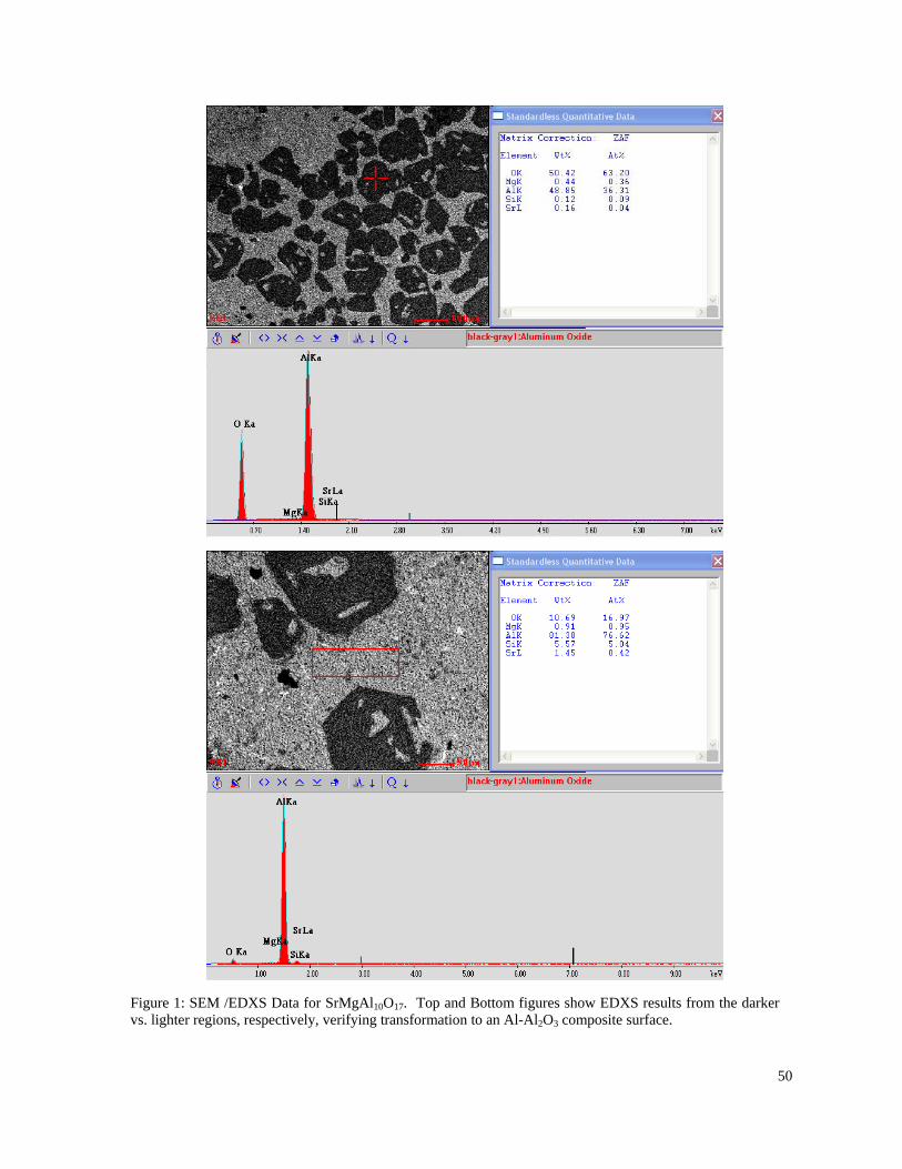
50

Figure 1: SEM /EDXS Data for SrMgAl10O17. Top and Bottom figures show EDXS results from the darker vs. lighter regions, respectively, verifying transformation to an Al-Al2O3 composite surface.