Abstract— Localization systems based on Received Signal

Strength Indicator (RSSI) exploit fingerprinting (based on

extensive signal strength measurements) to calibrate the system

parameters. This procedure is very expensive in terms of time as

it relies on human operators. In this paper we propose a virtual

calibration procedure which only exploits the measurements of

the RSSI between pairs of anchors. In particular we propose two

heuristics for virtual calibration and we evaluate their

performance with respect to an ad-hoc calibration campaign by

performing measures in an indoor environment with an IEEE

802.15.4 sensor network.1

I. INTRODUCTION

Localization is an important building block of context-aware

system as witnessed in [1]. The general solution based on

Global Positioning System (GPS) is unfortunately available

only in outdoor environments. In indoor environment a viable

solution to localization of users exploits wireless sensor

networks [2]. Sensor network-based solutions estimate the

(unknown) location of mobile sensors (placed on the users)

with respect to a set of fixed sensor (called anchors), whose

position is known, by estimating the distances between the

mobile node and a set of anchors. Once these distances are

known a standard multilateration technique or other methods

[3] can be used to determine the mobiles position. This means

that the localization problem reduces to the determination of

the distances between arbitrary pairs of sensor nodes. A

simple and widely used way to estimate distances is based on

RSSI [4-6] that does not require complex hardware. In [4] the

authors suggest that algorithms that estimate distances

between two wireless devices based on their reciprocal RSSI

are unable to capture the myriad of effects on signal

propagation in an indoor environment. Nevertheless, because

of RSSI does not require a special or a sophisticated hardware,

but rather it has become a standard feature in most wireless

devices, RSSI-based localization techniques have received

considerable research interest. As a matter of fact, in [5] the

authors have shown that despite the reputation of RSSI as a

coarse method to estimate range, it can achieve an accuracy of

about 1.5m RMS in a test bed experiment. Fading outliers can

still impair the RSSI relative location system, implying the

need for a robust estimator. A method to improve the quality

of localization exploiting a number of RSSI measurements

averaged in a time window to counteract interference and

fading has been proposed in [6]. Moreover, RSSI has been

1 Work founded in part by the European Commission in the framework of the

FP6 projects PERSONA (contract N. 045459) and INTERMEDIA (contract

N.38419)

used in the RADAR [7] and in the Cricket [8] systems that can

achieve a location granularity of 1.2 meters x 1.2meters.

The distance estimation techniques exploiting RSSI rely on a

radio propagation model. In indoor environment these models

also take into account parameters such as the wall attenuation

factor (WAF) and floor attenuation factors (FAF) to model the

effect of walls and floors on the radio waves. Unfortunately,

RSSI is environment dependent, moreover in indoor

environments, the wireless channel is very noisy and the radio

frequency signal can suffer from reflection, diffraction and

multipath effect, which makes the signal strength a complex

function of distance. To overcome these problems, wireless

location systems uses a priori calibration of the propagation

model (called fingerprinting). This calibration works in two

phases: the training phase and the estimation phase. In the

training phase it is measured the RSSI at a grid of points in the

area of interest, and in the estimation phase this information is

used to estimate the propagation model parameters. Clearly,

the accuracy of the calibration procedure depends on the

number of points in the grid and to the number of measures

taken per point. This procedure is very expensive in terms of

time as it requires human intervention, which is a practical

barrier to its wider adoption.

In this paper we use the same propagation model proposed in

[3] which we assume to be valid, and we consider a virtual

calibration procedure which only exploits the measures of the

RSSI between pairs of anchors. In particular we propose two

heuristics for virtual calibration and we evaluate their

performance with respect to an ad-hoc calibration campaign

by performing measures in an indoor environment with an

IEEE 802.15.4 sensor network. We show that the performance

of virtual calibration in terms of accuracy of the estimated

distances is close to that achievable with more expensive, ad-

hoc calibration procedures, and it is thus a viable alternative to

simplify the calibration of a localization system.

II. THE WIRELESS SYSTEM MODEL

In this paper we assume a localization system comprising a set

of anchors A = {a1, a2… an}, a set of mobile nodes M = {m1,

m2… mp} and a localization server L. The anchors have well

known position on the map, identified by the pair (xi, yi). Each

anchor periodically emits a beacon packet containing its

identifier. The mobile nodes are those which need to be

localized by the system. To this purpose a mobile node

receives the beacons from the anchors, for each beacon

computes the corresponding RSSI, and sends to the

localization server the pair <RSSI, anchor id>. The

Virtual Calibration for RSSI-based Indoor

Localization with IEEE 802.15.4 Paolo Barsocchi

1, Stefano Lenzi

1, Stefano Chessa

1,2, Member, IEEE, Gaetano Giunta

1,3, Member IEEE

1ISTI-CNR, Pisa Research Area, Via G.Moruzzi 1, 56124 Pisa, Italy

2Computer Science Department, University of Pisa, Largo B. Pontecorvo 3, 56127 Pisa, Italy

3Department of Applied Electronics, University of Roma Tre, via Vasca Navale 84, 00146 Roma

localization server accumulates all the pairs of each mobile

node and estimates the position of the mobiles exploiting a

suitable propagation model.

The propagation model is used to calculate the expected RSSI

map of the building. The RSSI map is evaluated only for a

grid of points. For each point of the grid with coordinates (x,

y), the map provides an n-dimensional vector S(x,y)!"n

defined as S(x,y) = {s1, s2… sn} where si is the expected RSSI

value from anchor ai. Figure 1 shows an example of

deployment of the anchors in a building.

III. INDOOR PROPAGATION MODEL FOR IEEE 802.15.4

The large-scale path loss model considered in this paper is

summarized in this Section. Most researchers model the

indoor path loss with the one-slope model [5], which assumes

a linear dependence between the path loss (dB) and the

logarithm of the distance d between the transmitter and the

receiver:

L d( )db= l0 +10! log10 d( ) (1)

where l0 is the path loss at a reference distance of 1 meter

(thought the paper we express distances in meters) and ! is the

power decay index (also called path loss exponent). A

generalization of the one-slope model is the two-slope model

suggested by [9] to approximate the two-ray propagation

model.

The two-slope model is characterized by a break point that

separates the various properties of propagation in near and far

regions relative to the transmitter. In fact, the path loss

exponent changes when the distance d is greater than the

break point. In particular, the authors in [9] describe the

existence of a transition region where the break point b is such

that: !h

thr

"< b <

4!hthr

" (2)

where ht is the transmitter antenna height, hr is the receiver

antenna height, and " is the wavelength of the radio signal.

However, in a typical sensor network scenario, the break point

distance is hundreds of meters, therefore in practice the one-

slope and the two-slope models are equivalent in indoor

scenarios where the rooms are only a few square meters in size.

Although the one-slope model is simple to use, it does not

adequately account for the propagation characteristics in

indoor environments. In fact, a further generalization of the

one-slope model consists in adding an attenuation term due to

losses introduced by walls and floors penetrated by the direct

path:

L d( )db= l0 +10! log10 d( ) +WAF + FAF (3)

where FAF is the floor attenuation factor and WAF is the wall

attenuation factor expressed as:

WAF = kili

i=1

N

! (4)

where ki is the number of penetrated walls of type i, and li is

the attenuation due to the wall of type i. Since the sensor

devices were located on the same floor, the attenuation term

due to the propagation among different floors was not

included in (3).

A similar model was proposed in [3]. In their model they

introduce a multi-wall component. This factor also includes

the number of normal and fireproof doors and their status

(open/closed) met by the direct paths.

We observe that these parameters are important for the IEEE

802.11 based localization, due to the lower density of the

Access Points (the anchors of the system) deployed in the

indoor environment. This result in a cumbersome system to

handle for the end-user, since the status of the doors needs to

be frequently updated. In our case we deal with a high anchor

density and the anchors have a reduced radio communication

range, thus the number of doors affecting direct paths is very

low. For this reason we neglect the door status and we use a

simplified model.

IV. CALIBRATION PROCEDURES

The objective of the calibration is to adapt the theoretical

propagation model to the environment where it is actually

used. Due to the dynamics of the channel, which essentially capture the spatial-temporal variations of wireless fading events, an automatic calibration procedure increases the

performance of the localization systems. Virtual calibration

procedure achieves this goal without human intervention, by

exploiting only information obtained from the anchors. In

particular, the anchors preliminary exchange beacons to

compute reciprocal RSSI and the localization server uses this

information to configure the parameters of the theoretical

propagation model.

The parameters of the propagation model (3) are: l0 (the path

loss at distance of 1 meter), ! (the air attenuation factor), and li

(the attenuation factor for the wall of type i). Since l0 should

be estimated in a free space and it is not affected by the

environment, it only depends on physical properties of the

devices hardware and it can be estimated a priori, thus it is not

object of virtual calibration.

To calibrate parameters ! and li we propose two heuristics:

global virtual calibration (G-procedure) and per-wall virtual

calibration (W-procedure) comparing these with an ad-hoc

calibration (H-procedure). G-procedure assigns the same

parameters for every wall, based on all RSSI measures

obtained from any pair of anchors. Instead, W-procedure

provides an attenuation factor for the walls that directly affect

the communication between specific pairs of anchors, and it

uses G-procedure for all the other walls. The H-procedure,

which has been used in many previous works [5, 10], exploits

Fig. 1. Map of the building used for the experiments.

the RSSI measurements on a grid of points in the environment

to estimate the propagation model parameters.

Hereafter we use the following notation:

! C = {(ai, aj)!A : ai and aj can communicate directly}

! Ri = {aj1, aj2,…, ajn} is the set containing the id of all

anchors in the same room, hence "(a, b) ! Ri : a#b the

communication between a and b is “wall-free”;

! Wn is the set of all pairs (ai,aj) such that the communication

channel between ai and aj crosses exactly n wall(s);

A. Global virtual calibration

The G-procedure considers a single virtual type of wall. This

leads (3) to:

L(d)db= l0 +10! log10 d( ) + klw (5)

where k identifies the number of wall crossed by the signal

and lw is the attenuation introduced by the wall on the signal.

During the virtual calibration phase we can estimate all the

required parameters (l0, !, lw).

Substituting d(i,j) as actual distance between anchors ai and aj,

and k(i,j) as the number of wall crossed by the direct path

between anchors ai and aj in (5), we want to obtain an

estimation RSSI"(i,j) of actual RSSI:

RSS ! I i ,j( ) = l0 "10# log10 d

i ,j( )( ) + ki ,j( ) lw

$i, j : ai ,a j( ) % C (6)

The estimated RSSI"(i,j) differs from the measured RSSI(i,j) by

an error component #(i,j). We assume that all #(i,j) are identically

distributed and uncorrelated among themselves. Recalling that

l0 is estimate a priori (see Section IV), and according to [11],

the approximation of the remaining parameters (!,lw) that

minimizes the least mean square error !RSSI " RSSI"!2 can be

achieved by direct method. The computation cost for direct

method solving a linear least mean square estimator problem

is polynomial [11].

B. Per-wall virtual calibration

With this technique we estimate an individual attenuation

factor for each wall between any pair of anchors belonging to

C. Let us assume there are q different types of wall in the map

of the building and let F = {f1, f2… fq} the set of attenuation

factors for each type of wall. Thus the equation (6) building

the linear system becomes:

RSS ! I i ,j( ) = l0 "10# log10 d

i ,j( )( ) + kh i ,j( ) fh

h=1

q

$

%i, j : ai ,a j( ) & C

(7)

where kh(i,j) is the wall number of type h crossed by signal

considering the direct path anchors ai and aj in (5). The path

loss exponent ! used in this equation is previously evaluated

with the G-procedure. Instead the evaluation of parameters fi

!F is achieved with the same methodology used in Subsection

A, by means of the least mean square estimator.

V. SIMULATION AND RESULTS

As observed in [3] the measured RSSI is function of the path

loss and of the wall attenuation factor, which can be estimated

with the above calibration technique. Furthermore, transmit

powers will vary as batteries become depleted. This implies

that the parameters change during the sensors’ lifetime.

In this section we present the results of a measurement

campaign aimed at comparing the performance of the three

heuristics proposed in the previous section.

We performed a two phases of measurements, each aimed at

(1) performing the calibration of the propagation model using

the three different procedure, namely: H-procedure, G-

procedure, and W-procedure, and (2) measuring the RSSI on a

grid of points in the environment, to compare the localization

error performance of the procedures.

We use the H-procedure as reference technique, and we

evaluate the performance of the two virtual calibration

techniques in terms of the following formula:

!G = stdclb RSSI( ) " slfclbG RSSI( )2 (8)

!W = stdclb RSSI( ) " slfclbW RSSI( )2 (9)

Where stdclb is the function computing the distance based on

the propagation model calibrated with H-procedure, slfclbG

provides the distance by means of the propagation model

calibrated with G-procedure and slfclbW provides the distance

by means of the propagation model calibrated with W-

procedure.

In order to gather a better view of the comparison we studied

the Probability Density Function (PDF) of !G and !W the

errors. Based on the set of all the RSSI measured between the

communications from anchors to mobile, produced during the

second phase of the measuring campaign, we estimated the

PDF error as the frequency of the error affecting the estimated

distance. In the next subsection we present the setup of our

experiment and the results of the comparison between our

techniques.

A. Experimental setup

We performed the experiments in our laboratory. It is a typical

office environment with an area of approximately 7m by 11m.

It has desks, chairs, cabinets, computers, monitors, etc. This

environment is harsh for wireless communication due to

multi-path reflections from walls and the possibility of

interference from electronic devices. Figure 1 shows the

layout of the laboratory and the deployment of the anchors in

the rooms.

For the experiments we used a Sensor Network of 7 MicaZ

[12] which uses the Chipcom CC2420 radio subsystem

implementing the IEEE 802.15.4 standard. The experiments

consist in a set of measures between a pair of anchors or

between an anchor and a point of the grid (in case of ad-hoc

calibration). Each measure collects 300 RSSIs, where every

RSSI is averaged over a set of 100 samples. Each sample is

obtained exchanging a beacon packet between two sensors

every 1/32 second, using the highest transmission power of the

MicaZ.

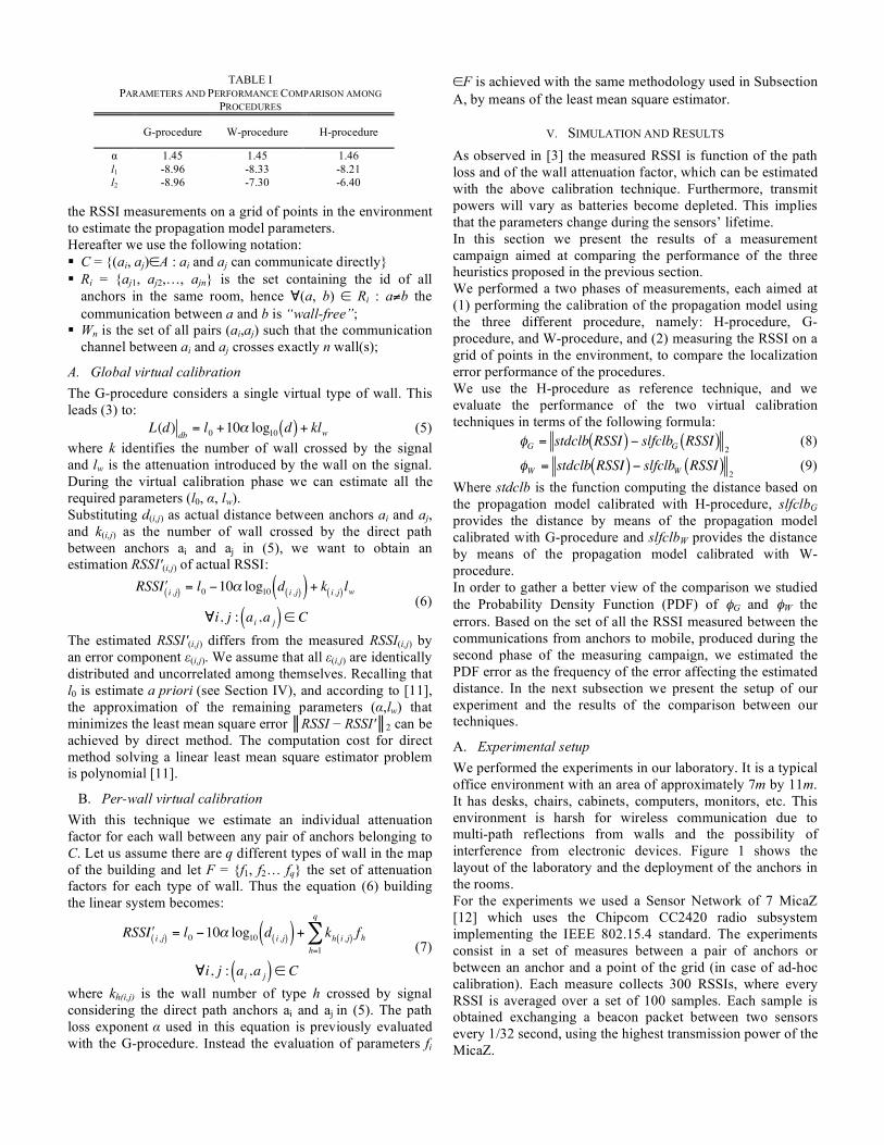
TABLE I

PARAMETERS AND PERFORMANCE COMPARISON AMONG

PROCEDURES

G-procedure W-procedure H-procedure

# 1.45 1.45 1.46

l1 -8.96 -8.33 -8.21

l2 -8.96 -7.30 -6.40

As mentioned in Section IV the l0 parameter can be estimated

a priori as the path loss at a reference distance. To this

purpose we preliminary evaluated l0 measuring the RSSI

between two anchors deployed at 1 meter distance, obtaining

l0 = !10.06.

We preliminary executed the H-procedure to obtain the

reference parameters of the propagation model to be used for

the comparison with G-procedure and W-procedure

techniques. In particular we estimated ! = 1.46, l1 = !8.21dB,

l2 = !6.4dB. The parameters obtained with all the calibration

methods are shown in Table I.

During our experiments we observed the typical features of

radio channels [13]: Asymmetrical links (the connectivity from

node A to node B might be different than that from node B to

node A), Non-isotropic connectivity (the connectivity is not

necessarily the same in all the directions from the source), and

Non-monotonic distance decay (nodes that are far away from

the source may have better connectivity than nodes that are

closer). Note that non-monotonic distance decay is the main

cause of localization error.

B. Global virtual calibration performance

With Global virtual calibration (G-procedure) the estimated

parameters are " = 1.45 and l1 = l2 = lw = !8.96dB. Figure 2

shows the results obtained in a single room, without the

attenuation introduced by the walls (WAF = 0). In particular,

Figure 2 shows the received power measured from the mobile.

The dotted line is the H-procedure, and the solid line is G-

procedure. As we can see from the figure, the two lines are

practically overlapped due to the optimal fit of both lines, with

the real path loss exponent. Consequently, the error of G-

procedure with respect to the H-procedure !G is negligible.

Figure 3 shows the PDF of !G for measures obtained in the

whole environment (WAF!0). In this case the error is less then

1.5m in the 90% of the cases. This result is due to the fact that

the attenuation factor of both walls has been forced to be the

same.

Consider that, from the measures in our environment, the H-

procedure is affected by an error of about 1.5m. Thus, the

error of 1.5m of the G-procedure with respect to the H-

procedure can be considered acceptable since it fits the highest

precision achievable in our environment.

C. Per-wall virtual calibration performance

With W-procedure the estimated parameters are "= 1.45,

l1=!8.33dB, and l2=!7.3dB. The main difficulty for this

calibration method is due to the different number of sample

used to estimate the single wall attenuation. In our case we

have 5 anchors to estimate the first wall and other 3 anchors

for the second one. Therefore, in order to resolve the Equation

(7) with the least mean square estimator, we weigh the WAF

parameters with a number directly proportional to the number

of established links between pairs of anchors and inversely

proportional to the number of anchors.

Figure 4 shows the PDF of !W. It is seen that virtual

calibration of individual walls improves the performance of

virtual calibration; in particular comparing the W-procedure

with the H-procedure we observed an error less than 1.5m in

the 98% of the cases. This is a significant improvement over

G-procedure. Table II summarize the results obtained showing

the Cumulative Distribution Function (CDF) of !G and !W.

This table highlight that the W-procedure increase the

performance with respect to the G-procedure. Not surprisingly,

the W-procedure outperforms the G-procedure, due to the

better accuracy in the walls modeling.

To measure the performance of the two virtual calibration

procedure (G-procedure and W-procedure) with respect to the H-

procedure we evaluated the localization error. The metric

chosen to measure the performance considers the localization

error between our novel calibration procedure and the

conventional H-procedure with a fixed localization algorithm. The localization algorithm selected is based on the RF map of the area. The RF map is a database containing the estimated receiver power from each anchors for each point (x, y) positioned over a regular grid. The RF map covers the entire area and it has been generated using the estimated parameters for each virtual calibration procedure. The RSSIs measured by

TABLE II

CDF OF THE ERRORS

Error [m] CDF of !G CDF of !W

0.25 0.604 0.896

0.5 0.732 0.919

1 0.868 0.973

1.5 0.901 0.984

-28-26-24-22-20-18-16-14-12-10

-8-6

1 10

RSS

I [dB

]

distance [m]

Theoretical model and measured performanceH-procedureG-procedure

Fig. 2. Received RSSI measured from the mobile node.

0 0.02 0.04 0.06 0.08

0.1 0.12 0.14 0.16 0.18

0.2

0 0.2 0.4 0.6 0.8 1 1.2 1.4

Prob

abilit

y

meters

PDF of !G

Fig. 3. PDF of !G considering all the measured data.

the mobile (received by the anchors) is compared to the data stored in an RF map of the area to discriminate the position of the mobile. Indicating with w = (w1,w2 ...wn) the vector of the measured power, it is compared to the stored power vectors W(i,j) = (W(i,j)1,W(i,j)2 ... W(i,j)n), for each (i,j) contained in the RF map. The vector W(i,j) contains the estimated powers we aspect to received (in respect to the signal propagation model chosen) on the (xi, yj) point from the anchors. The point on the RF map resulting in the minimum distance from w is selected as the position of the mobile. From the work in [7], the Euclidean metric gives better results with respect to the other methods. Considering that the mobile is positioned in the (xi, yj ) point of the RF map, the definition of

our localization results in (i,j)=arg{min(h,k)!NxM!w–W(h,k)!2},

where N is the set {1,2 ... n} with n the number of rows, and M is the set {1,2 ... m} with m the number of columns.

Figure 5 shows the Cumulative Distribution Function

obtained by using the above mentioned localization algorithm

for each calibration procedure.

Other localization algorithms based on RF map can be used to

localize the mobile node. We fixed a simple localization

algorithm to demonstrate that our virtual calibration procedure

performs mostly like other ad-hoc calibration procedures which

requires a measurement campaigns that are time consuming

and in general expensive.

As depicted in Figure 5 the G-procedure performs like the

commonly used H-procedure, in terms of localization error. In

fact, it is worth to note that, the CFD of the W-procedure is

identical to the H-procedure one, thus it is mostly hidden in

the graph. This means that virtual calibration procedure results

in the same localization error like the expensive ad-hoc

calibration procedure.

VI. CONCLUSIONS

We proposed a virtual calibration procedure for localization

that only exploits RSSI measurements between pairs of

anchors. In particular, we propose two heuristics for virtual

calibration and evaluate their performance with respect to

fingerprinting in indoor environments with IEEE 802.15.4

sensor network. We showed that the performance of virtual

calibration, in terms of accuracy of the estimated distances, is

close to that achievable with more expensive fingerprinting.

The proposed method is thus a viable alternative to simplify

the calibration of a localization system.

REFERENCES

[1] R. Want et.al., “The Active Badge Location System” ACM Transactions

on Information Systems, 10(1):91- 102, 1992

[2] P. Baronti, et.al., “Wireless sensor networks: a survey on the state of the

art and the 802.15.4 and zigbee standards”, Computer Communications,

30:1655-1695, 2007

[3] Borrelli, A. et.al., “Channel models for IEEE 802.11b indoor system

design”, IEEE International Conference on Communications, pp 3701-

3705, 20-24 June 2004

[4] E. Elnahrawy, X. Li, and R. Martin, “The limits of localization using

signal strength: a comparative study”, in First Annual IEEE

Communications Society Conference Sensor and Ad Hoc

Communications and Networks, 2004, pp. 406-414.

[5] N. Patwari et.al., “Relative location estimation in wireless sensor

networks”, IEEE Transactions on Signal Processing, vol. 51, no. 8, pp.

2137-2148, 2003.

[6] P. Bergamo and G. Mazzini, “Localization in sensor networks with

fading and mobility”, in the 13th IEEE International Symposium on

Personal, Indoor and Mobile Radio Communications, vol. 2, 2002, pp.

750-754.

[7] P. Bahl, V.N. Padmanabhan, “RADAR: An in-building RF- based user

location and tracking system”, in Proceedings of IEEE Infocom, Tel

Aviv, Israel, 2000.

[8] N. Pryiantha, A. Chakaborty, H. Balakrishnan, “The Cricket location

support system”, in Proceedings of ACM MobiComm 2000, pp. 32-43,

Boston, Massachussetts, 2000.

[9] E.Green and M. Hata, “Microcellular propagation measurements in a

urban environment” in proc. PIMRC, pp. 324-328, Sept. 1991

[10] D. Lymberopoulos, Q. Lindsey, and A. Savvides, “An empirical analysis

of radio signal strength variability in IEEE 802.15.4 networks using

monopole antennas,” Yale ENALAB Technical Report 050501, 2005.

[11] Ake Bjorck, “Solution of Equations in RN”, vol. 1, NorthHolland, 1990

[12] Crossbow Technology Inc., http://www.xbow.com.

[13] D. Ganesan et.al., “Complex Behavior at Scale: An Experimental Study

of Low-Power Wireless Sensor Networks”, Technical Report CSDTR

02-0013, UCLA, February 2002.

0

0.05

0.1

0.15

0.2

0.25

0.3

0 0.2 0.4 0.6 0.8 1 1.2 1.4

Prob

abilit

y

meters

PDF of !W

Fig. 4. PDF of !W considering all the measured data.

100 150 200 250 300 350 400 450 5000

0.1

0.2

0.3

0.4

0.5

0.6

0.7

0.8

0.9

1

Error [cm]

F(x

)

CDF comparison

G−procedureH−procedureW−procedure

Fig. 5. Localization error using the Euclidean metric with the H, G, and W-procedures.