© 2008 Matthieu Maitre

“TRAVELLING WITHOUT MOVING”:A STUDY ON THE RECONSTRUCTION, COMPRESSION, ANDRENDERING OF 3D ENVIRONMENTS FOR TELEPRESENCE

BY

MATTHIEU MAITRE

Diplome d’ingenieur, Ecole Nationale Superieure de Telecommunications, 2002M.S., University of Illinois at Urbana-Champaign, 2002

DISSERTATION

Submitted in partial fulfillment of the requirementsfor the degree of Doctor of Philosophy in Electrical and Computer Engineering

in the Graduate College of theUniversity of Illinois at Urbana-Champaign, 2008

Urbana, Illinois

Doctoral Committee:

Assistant Professor Minh N. Do, ChairYoshihisa Shinagawa, Siemens Medical Solutions USA, IncProfessor Douglas L. JonesProfessor Thomas HuangProfessor Narendra Ahuja

ABSTRACT

In this dissertation, we study issues related to free-view 3D-video, and in partic-

ular issues of 3D scene reconstruction, compression, and rendering. We present

four main contributions. First, we present a novel algorithm which performs sur-

face reconstruction from planar arrays of cameras and generates dense depth maps

with multiple values per pixel. Second, we introduce a novel codec for the static

depth-image-based representation, which jointly estimates and encodes the un-

known depth map from multiple views using a novel rate-distortion optimization

scheme. Third, we propose a second novel codec for the static depth-image-based

representation, which relies on a shape-adaptive wavelet transform and an ex-

plicit representation of the locations of major depth edges to achieve major rate-

distortion gains. Finally, we propose a novel algorithm to extract the side infor-

mation in the context of distributed video coding of 3D scenes.

ii

To my families.

iii

ACKNOWLEDGMENTS

This thesis would not have been possible without the help and inspiration from

many people. First and foremost I would like to thank my thesis advisers, Profes-

sors Minh N. Do and Yoshihisa Shinagawa, for their guidance and precious advice

during the course of this study. I am also grateful to my committee members –

Professors Thomas Huang, Narendra Ahuja, and Douglas L. Jones – for the help

they gave me in defining the scope of this thesis.

I would like to thank the mentors I had the pleasure to work with during my

internships: Christine Guillemot and Luce Morin of the Irisa, and Michelle Yan,

Yunqiang Chen, and Tong Fang of Siemens Corporate Research (SCR).

I would like to express my appreciation to Jean Tourret, Robert West and

Professors Yizhou Yu, Bruce Hajek and Daniel M Liberzon for the suggestions they

offered me. I am grateful to my labmates at the Coordinated Science Laboratory

(CSL), the Beckman Institute, SCR, and Irisa for their assistance and friendships,

which made my stay in all these places most enjoyable.

I am also indebted to the staff of the Beckman Institute and CSL, and in

particular to John M. Hart, Barbara Horner, and Dan R. Jordan, for having taken

care of so many material details that made my work much easier. I would also like

to express my gratitude to the University of Illinois in general, for providing such

a rich and fulfilling research environment.

Although I never had the pleasure to meet them in person, I am grateful to

Frank Herbert [1] and Jamiroquai [2] for helping me find a title for this thesis.

iv

Finally, on the personal side, I would like to thank my three families: my wife,

for her love and patience; my parents and sister, for their constant encouragement;

and my parents-in-law, for all the enjoyable moments I spend with them.

v

TABLE OF CONTENTS

LIST OF TABLES . . . . . . . . . . . . . . . . . . . . . . . . . . . . ix

LIST OF FIGURES . . . . . . . . . . . . . . . . . . . . . . . . . . . x

CHAPTER 1 INTRODUCTION . . . . . . . . . . . . . . . . . . . 11.1 Motivation . . . . . . . . . . . . . . . . . . . . . . . . . . . . . . . . 11.2 Problem Statement . . . . . . . . . . . . . . . . . . . . . . . . . . . 31.3 Prior Art . . . . . . . . . . . . . . . . . . . . . . . . . . . . . . . . 51.4 Thesis Outline . . . . . . . . . . . . . . . . . . . . . . . . . . . . . . 5

CHAPTER 2 SYMMETRIC STEREO RECONSTRUCTIONFROM PLANAR CAMERA ARRAYS . . . . . . . . . . . . . . 82.1 Introduction . . . . . . . . . . . . . . . . . . . . . . . . . . . . . . . 82.2 Relation to Previous Work . . . . . . . . . . . . . . . . . . . . . . . 92.3 The Rectified Space . . . . . . . . . . . . . . . . . . . . . . . . . . . 11

2.3.1 Overview . . . . . . . . . . . . . . . . . . . . . . . . . . . . 112.3.2 Rectification homographies . . . . . . . . . . . . . . . . . . . 13

2.4 Stereo Reconstruction . . . . . . . . . . . . . . . . . . . . . . . . . 152.4.1 Overview . . . . . . . . . . . . . . . . . . . . . . . . . . . . 152.4.2 Geometric cost volume G(m,n) . . . . . . . . . . . . . . . . . 182.4.3 Photometric cost volume P (m,n) . . . . . . . . . . . . . . . . 19

2.5 Global Surface Representation . . . . . . . . . . . . . . . . . . . . . 222.5.1 Layered depth image . . . . . . . . . . . . . . . . . . . . . . 222.5.2 Sprites with depth . . . . . . . . . . . . . . . . . . . . . . . 23

2.6 Experimental Results . . . . . . . . . . . . . . . . . . . . . . . . . . 252.7 Conclusion . . . . . . . . . . . . . . . . . . . . . . . . . . . . . . . . 30

CHAPTER 3 WAVELET-BASED JOINT ESTIMATION ANDENCODING OF DIBR . . . . . . . . . . . . . . . . . . . . . . . 313.1 Introduction . . . . . . . . . . . . . . . . . . . . . . . . . . . . . . . 313.2 Problem Formulation . . . . . . . . . . . . . . . . . . . . . . . . . . 353.3 Rate-Distortion Optimization . . . . . . . . . . . . . . . . . . . . . 41

3.3.1 Overview . . . . . . . . . . . . . . . . . . . . . . . . . . . . 413.3.2 Reference view . . . . . . . . . . . . . . . . . . . . . . . . . 423.3.3 One-dimensional disparity map . . . . . . . . . . . . . . . . 43

vi

3.3.4 Dynamic programming . . . . . . . . . . . . . . . . . . . . . 463.3.5 Two-dimensional disparity map . . . . . . . . . . . . . . . . 513.3.6 Bitrate optimization . . . . . . . . . . . . . . . . . . . . . . 533.3.7 Quality scalability . . . . . . . . . . . . . . . . . . . . . . . 54

3.4 Experimental Results . . . . . . . . . . . . . . . . . . . . . . . . . . 553.5 Conclusion . . . . . . . . . . . . . . . . . . . . . . . . . . . . . . . . 64

CHAPTER 4 JOINT ENCODING OF THE DIBR USING SHAPE-ADAPTIVE WAVELETS . . . . . . . . . . . . . . . . . . . . . . 654.1 Introduction . . . . . . . . . . . . . . . . . . . . . . . . . . . . . . . 654.2 Proposed Codec . . . . . . . . . . . . . . . . . . . . . . . . . . . . . 674.3 Shape-Adaptive Wavelet Transform . . . . . . . . . . . . . . . . . . 684.4 Lifting Edge Handling . . . . . . . . . . . . . . . . . . . . . . . . . 724.5 Edge Representation and Coding . . . . . . . . . . . . . . . . . . . 734.6 Experimental Results . . . . . . . . . . . . . . . . . . . . . . . . . . 754.7 Conclusion . . . . . . . . . . . . . . . . . . . . . . . . . . . . . . . . 77

CHAPTER 5 3D MODEL-BASED FRAME INTERPOLATIONFOR DVC . . . . . . . . . . . . . . . . . . . . . . . . . . . . . . . 795.1 Introduction . . . . . . . . . . . . . . . . . . . . . . . . . . . . . . . 795.2 3D Model Construction . . . . . . . . . . . . . . . . . . . . . . . . . 82

5.2.1 Overview . . . . . . . . . . . . . . . . . . . . . . . . . . . . 825.2.2 Notation . . . . . . . . . . . . . . . . . . . . . . . . . . . . . 835.2.3 Camera parameter estimation . . . . . . . . . . . . . . . . . 845.2.4 Correspondence estimation . . . . . . . . . . . . . . . . . . . 875.2.5 Results . . . . . . . . . . . . . . . . . . . . . . . . . . . . . . 90

5.3 3D Model-Based Interpolation . . . . . . . . . . . . . . . . . . . . . 915.3.1 Projection-matrix interpolation . . . . . . . . . . . . . . . . 925.3.2 Frame interpolation based on epipolar blocks . . . . . . . . . 925.3.3 Frame interpolation based on 3D meshes . . . . . . . . . . . 945.3.4 Comparison of the motion models . . . . . . . . . . . . . . . 95

5.4 3D Model-Based Interpolation with Point Tracking . . . . . . . . . 975.4.1 Rationale . . . . . . . . . . . . . . . . . . . . . . . . . . . . 975.4.2 Tracking at the decoder . . . . . . . . . . . . . . . . . . . . 985.4.3 Tracking at the encoder . . . . . . . . . . . . . . . . . . . . 99

5.5 Experimental Results . . . . . . . . . . . . . . . . . . . . . . . . . . 1005.5.1 Frame interpolation without tracking (3D-DVC) . . . . . . . 1015.5.2 Frame interpolation with tracking at the encoder (3D-DVC-

TE) . . . . . . . . . . . . . . . . . . . . . . . . . . . . . . . 1025.5.3 Frame interpolation with tracking at the decoder (3D-DVC-

TD) . . . . . . . . . . . . . . . . . . . . . . . . . . . . . . . 1065.5.4 Rate-distortion performances . . . . . . . . . . . . . . . . . 107

5.6 Conclusion . . . . . . . . . . . . . . . . . . . . . . . . . . . . . . . . 1095.7 Acknowledgments . . . . . . . . . . . . . . . . . . . . . . . . . . . . 110

vii

CHAPTER 6 CONCLUSION . . . . . . . . . . . . . . . . . . . . . 111

APPENDIX A FIXING THE PROJECTIVE BASIS . . . . . . 112

APPENDIX B BUNDLE ADJUSTMENT . . . . . . . . . . . . . 113

APPENDIX C PUBLICATIONS . . . . . . . . . . . . . . . . . . 115C.1 Journals . . . . . . . . . . . . . . . . . . . . . . . . . . . . . . . . . 115C.2 Conferences . . . . . . . . . . . . . . . . . . . . . . . . . . . . . . . 115C.3 Research Reports . . . . . . . . . . . . . . . . . . . . . . . . . . . . 116

REFERENCES . . . . . . . . . . . . . . . . . . . . . . . . . . . . . . 117

AUTHOR’S BIOGRAPHY . . . . . . . . . . . . . . . . . . . . . . . 125

viii

LIST OF TABLES

2.1 Performances on the Middlebury dataset with two cameras (fromtop to bottom: percentage of erroneous disparities over all areasfor the proposed method, percentage for the best method on eachimage, and ranks of the proposed method). . . . . . . . . . . . . . . 27

2.2 Percentage of erroneous disparities over all areas on Tsukuba forseveral multicamera methods. The proposed method achieves com-petitive error rates and scales with the number of cameras. . . . . . 27

2.3 Number of disparity values in a standard disparity map and in anLDI, for various numbers of cameras on Tsukuba. Using an LDI and25 cameras increases the area of reconstructed surfaces by almost20%. . . . . . . . . . . . . . . . . . . . . . . . . . . . . . . . . . . . 29

3.1 Analysis and synthesis operators of the Laplace (L) and Sequential(S) transforms (see text for details). . . . . . . . . . . . . . . . . . . 44

5.1 Average PSNR (in dB) of interpolated frames using lossless keyframes. . . . . . . . . . . . . . . . . . . . . . . . . . . . . . . . . . . 104

ix

LIST OF FIGURES

1.1 Two state-of-the-art telepresence systems. This dissertation intro-duces methods aimed at enabling realistic, interactive, and large-scale telepresence systems (images reproduced from [3, 4]). . . . . . 2

1.2 Overview of the proposed 3D-video system. At each client, a 3Dscene is recorded by multiple cameras whose data is compressedusing images and depth models. This information is sent to thenetwork, along with data from other input devices. The networkaggregates across clients and performs physics-based simulation be-fore sending the data back to the clients. Each client then ren-ders the data and displays. Users are able to freely choose theviewpoint. . . . . . . . . . . . . . . . . . . . . . . . . . . . . . . . . 4

1.3 Research areas related to free-view 3D-video. . . . . . . . . . . . . . 5

2.1 A few rays of light in the rectified 3D space: rays passing throughthe optical centers of camera (0, 0) (a) and camera (1, 0) (b). Therays are aligned with the voxel grid, which simplifies visibility com-putations. . . . . . . . . . . . . . . . . . . . . . . . . . . . . . . . . 13

2.2 Rectification of four images from the toy sequence. After rectifica-tion, both the rows and the columns of the images are aligned. . . . 16

2.3 Camera MRF associated with a 2 × 4 camera array. Each noderepresents a camera with an observed image I and a hidden disparitymap D. Edges represent fusion functions. . . . . . . . . . . . . . . . 16

2.4 A simple example demonstrating the behavior of the occlusion model.Perfect disparity maps are obtained in two iterations. . . . . . . . . 20

2.5 Cropped disparity maps computed on Tsukuba with five camerasforming a cross. The proposed photometric cost reduces the dispar-ity errors due to partial occlusions. . . . . . . . . . . . . . . . . . . 20

2.6 The 3-layer LDI obtained on Tsukuba with 25 cameras. By treatingall the cameras symmetrically, the proposed algorithm recovers largeareas, which may be occluded in the central camera. . . . . . . . . . 22

2.7 Examples of sprites extracted from the LDI of Tsukuba with 25cameras. Note the absence of occlusion on the cans. . . . . . . . . . 24

2.8 Disparity map obtained from the four rectified images of the toysequence shown in Figure 2.2. . . . . . . . . . . . . . . . . . . . . . 25

x

2.9 Disparity maps obtained on the Middlebury dataset with two cam-eras. The occlusion model leads to sharp and accurate depth dis-continuities. . . . . . . . . . . . . . . . . . . . . . . . . . . . . . . . 26

2.10 Number of disparity values per pixel on Tsukuba (black: no value,white: 3 values). The area of the reconstructed surfaces increaseswith the number of cameras. . . . . . . . . . . . . . . . . . . . . . . 28

2.11 Cropped textures extracted from the LDIs of Tsukuba. Occlusionsshrink when the number of cameras increases. . . . . . . . . . . . . 29

3.1 Overview of the proposed codec: the encoder takes multiple viewsand jointly estimates and encodes a depth map together with areference image (the DIBR). The output DIBR can be used to renderfree viewpoints. . . . . . . . . . . . . . . . . . . . . . . . . . . . . . 34

3.2 The spatial extent of a ROI (sphere) with one pair of image anddepth map, along with seven views (cones). The central dark conedesignates the reference view. The planes represent iso-depth sur-faces (3D model reproduced with permission from Google 3D Ware-house). . . . . . . . . . . . . . . . . . . . . . . . . . . . . . . . . . . 37

3.3 The projection of an iso-depth plane onto two views gives rise to amotion field between the two which is a 2D homography. . . . . . . 38

3.4 An error matrix E from the Tsukuba image set with two optimalpaths overlaid, λ = 0 (dashed) and λ = ∞ (solid). Lighter shadesof gray indicate larger squared intensity differences. . . . . . . . . . 44

3.5 Dependency graph of a three-level L transform. The coefficientsin bold are those included in the wavelet vector d. Gray nodesrepresent the MSE and rate terms of the RD optimization. Thedashed box highlights the two-level L transform associated with(3.22). . . . . . . . . . . . . . . . . . . . . . . . . . . . . . . . . . . 47

3.6 Dependency graph of a three-level S transform. The coefficientsin bold are those included in the wavelet vector d. Gray nodesrepresent the MSE and rate terms of the RD optimization. . . . . . 47

3.7 Two divisions of the frequency plane and the associated graphs ofdependencies between the coefficients of the S transform. . . . . . . 52

3.8 The two sets of images used in the experiments. . . . . . . . . . . . 563.9 Disparity map of the Teddy set at four resolution levels, showing

the resolution scalability of the wavelet-based representation. . . . . 573.10 The DIBR of the Teddy set at three RD slopes corresponding to

reference-view bitrates of 0.1 bpp, 0.5 bpp, and 1.0 bpp (from leftto right). The S and L transforms generate disparity maps thatdegrade gracefully with the bitrate and contain less spurious noisethan quadtrees or blocks. . . . . . . . . . . . . . . . . . . . . . . . . 59

xi

3.11 The DIBR of the Tsukuba set at three RD slopes corresponding toreference-view bitrates of 0.1 bpp, 0.5 bpp, and 1.0 bpp (from leftto right). The S and L transforms generate disparity maps thatdegrade gracefully with the bitrate and contain less spurious noisethan quadtrees or blocks. . . . . . . . . . . . . . . . . . . . . . . . . 60

3.12 Views synthesized from the DIBR with a reference view encoded at0.5 bpp and differences with the original views. At low quantizationnoise, the errors are mostly due to occlusions and disocclusions. . . 61

3.13 Rate-distortion performances of the encoders based on wavelets (Sand L transforms), quadtrees, and blocks. Wavelets are superior toquadtrees and blocks in the case of larger disparity ranges. . . . . . 62

3.14 RD loss due to quality-scalable coding. The loss remains limitedover the whole range of bitrates. . . . . . . . . . . . . . . . . . . . . 63

3.15 Fraction of the bitrate allocated to the disparity maps. Except atvery low bitrates, the rate ratios are stable with values between 13%and 23%. . . . . . . . . . . . . . . . . . . . . . . . . . . . . . . . . . 63

4.1 Input data of the proposed DIBR codec: shared edges superimposedover a depth map (a) and an image (b). . . . . . . . . . . . . . . . . 66

4.2 Overview of the proposed encoder. It relies on a SA-DWT and anedge coder (gray boxes) to reduce data correlations, both withinand between the image and the depth map. . . . . . . . . . . . . . 68

4.3 Comparison of standard and shape adaptive DWTs. In the lattercase, all but the coarsest high-pass band are zero. . . . . . . . . . . 70

4.4 The four lifting steps associated with a 9/7 wavelet, which trans-form the signal x first into a and then into y. The values x2t+2

and a2t+2 on the other side of the edge (dashed vertical line) areextrapolated. They have dependencies with the values inside thetwo dashed triangles. . . . . . . . . . . . . . . . . . . . . . . . . . . 71

4.5 Example of the dual lattices of samples and edges. Each edge in-dicates the statistical independence of the two half rows or halfcolumns of samples it separates. . . . . . . . . . . . . . . . . . . . . 74

4.6 Absolute values of the high-pass coefficients of the depth map usingstandard and shape-adaptive wavelets. The latter provides a muchsparser decomposition. . . . . . . . . . . . . . . . . . . . . . . . . . 76

4.7 Reconstruction of the depth map at 0.04 bpp using standard andshape-adaptive wavelets. The latter gives sharp edges free of Gibbsartifacts. . . . . . . . . . . . . . . . . . . . . . . . . . . . . . . . . . 77

4.8 Rate-distortion performances of standard and shape-adaptive wave-lets. The latter gives PSNR gains of up to 5.46 dB on the depthmap and 0.19 dB on the image. . . . . . . . . . . . . . . . . . . . . 78

5.1 Outline of the codec without point tracking (3D-DVC). The pro-posed codec benefits from an improved motion estimation and frameinterpolation (gray boxes). . . . . . . . . . . . . . . . . . . . . . . . 83

xii

5.2 Outline of the 3D model construction. . . . . . . . . . . . . . . . . 835.3 Correspondences and epipolar geometry between the two first loss-

less key frames of the sequences street and stairway. Feature pointsare represented by red dots, motion vectors by magenta lines endingat feature points, and epipolar lines by green lines centered at thefeature points. . . . . . . . . . . . . . . . . . . . . . . . . . . . . . . 91

5.4 Trifocal transfer for epipolar block interpolation. . . . . . . . . . . . 935.5 Outline of the frame interpolation based on epipolar blocks. . . . . 945.6 Outline of the frame interpolation based on 3D meshes. . . . . . . . 955.7 Norm of the motion vectors between the first two lossless key frames

of the stairway sequence for epipolar block matching (a), 3D meshfitting (b), and classical 2D block matching (c). . . . . . . . . . . . 96

5.8 Outline of the codec with tracking at the decoder (3D-DVC-TD). . 985.9 Outline of the codec with tracking at the encoder (3D-DVC-TE). . 995.10 Correspondences and epipolar geometry between the two first key

frames of the sequence statue. Feature points are represented byred dots, motion vectors by magenta lines ending at feature points,and epipolar lines by green lines centered at the feature points. . . . 101

5.11 PSNR of interpolated frames using lossless key frames (from topto bottom: sequences street, stairway, and statue). Missing pointscorrespond to key frames (infinite PSNR). . . . . . . . . . . . . . . 103

5.12 Correlation noise for GOP 1, frame 5 (center of the GOP) of thestairway sequence, using lossless key frames: 2D-DVC with classicalblock matching (a), 3D-DVC with mesh model and linear tracks (b),3D-DVC-TE with mesh model and tracking at the encoder (c), and3D-DVC-TD with mesh model and tracking at the decoder (d). Thecorrelation noise is the difference between the interpolated frame andthe actual WZ frame. . . . . . . . . . . . . . . . . . . . . . . . . . . 104

5.13 PSNR of key frames and interpolated frames of the street sequenceusing 3D-DVC-TE with mesh fitting on lossy key frames. Peakscorrespond to key frames. . . . . . . . . . . . . . . . . . . . . . . . 105

5.14 Variation of the subjective quality at QP = 26 between a key frame(frame 1) and an interpolated frame (frame 5). In spite of a PSNRdrop of 8.1 dB, both frames have a similar subjective quality. . . . . 106

5.15 Rate-distortion curves for H.264/AVC intra, H.264/AVC inter-IPPPwith null motion vectors, H.264/AVC inter-IPPP, 2D-DVC I-WZ-I, and the three proposed 3D codecs (top left: street, top right:stairway, bottom: statue). . . . . . . . . . . . . . . . . . . . . . . . 108

xiii

CHAPTER 1

INTRODUCTION

1.1 Motivation

Travel by physical motion was the only way human beings originally had to ex-

perience and modify the world that surrounded them. However, physical motion

suffers from several issues, the most conspicuous one probably being its slow speed.

Even using the fastest planes, intercontinental flights still take several hours. Fa-

tigue is also an issue. Long-haul travelers suffer from jet lag, and drivers lose their

attention after just a few hours of driving. Moreover, physical motion has high

energetic requirements, especially from fossil fuels, which strain environmental and

geopolitical equilibria.

Traveling without moving [1,2] – that is, being able to go to any place instantly

– would solve all these issues. Unfortunately, this has so far only been possible in

works of fiction [1]. The next best thing is then virtual travel, where a proxy, say

eletromagnetic waves, moves while we stay in place. This is the fundamental idea

behind telecommunication.

Through inventions like the telegraph, the telephone, the television, and the

internet, to name a few, our ability to shift stimuli like sound and light from one

place to another has been greatly improved. It has reached a point where both

places, the local one and the distant one, can look as if they only formed one,

like in the teleconference system shown in Figure 1.1(a). We are therefore getting

1

(a) HP’s Halo: a highly realistic system withlimited interactivity within room-size worlds.

(b) Linden Lab’s Second Life: a highly in-teractive system with limited realism withinlarge-scale worlds.

Figure 1.1: Two state-of-the-art telepresence systems. This dissertation intro-duces methods aimed at enabling realistic, interactive, and large-scale telepresencesystems (images reproduced from [3, 4]).

closer to a complete telepresence experience, in which it would not be possible to

distinguish the real world from its reproduced version.

At least three shortcomings remain in current telepresence technologies. First,

they are not able to convey stereopsis, that is, the sensation of depth. Videos are

still overwhelmingly limited to two spatial dimensions. Second, they do not offer

mobility. Users usually have to view the distant environment from a fixed point of

view, that of the camera, and cannot move inside this environment. Third, they

provide limited interactivity, only shifting stimuli from one place to another. A

full telepresence system would also shift actions, to let users modify the distant

environment.

These shortcomings would be simple to solve if the distant environment was

a virtual one, like those created for video games or the online 3D world shown

in Figure 1.1(b). In virtual environments, the stimuli delivered to the users are

rendered from a mathematical representation of these environments. Stereopsis

is then simply achieved by rendering from two slightly different points of view,

mobility amounts to applying a rigid transformation to the data, and interactivity

2

is obtained by simulating the laws of physics and transforming the data in an

appropriate manner.

Virtual environments have an additional advantage over real ones: the laws

of physics which govern them can be freely designed. They therefore offer new

possibilities, like providing safe learning environments where one can never get

hurt, be injured, or die. In such environments, professionals like surgeons, chemists,

firefighters, military personel, etc., can receive training which would not be possible

in the real world.

The shortcoming of existing virtual environments lies in their lack of realism:

they look too synthetic to make telepresence a believable experience. If we could

find a way to integrate the data from telepresence systems inside virtual environ-

ments, or at least the most important data, we would obtain a trade-off achieving

at the same time realism, stereopsis, mobility, and interactivity.

Developing such technologies would also be beneficial to other applications,

including 3D television. This recent televisual technology, which conveys stereopsis

to the viewers and may give some degree of freedom in the choice of the point of

view, is seen as the next evolution of television after high-definition. It has recently

received a lot of interest, both from the industry [5,6], academic institutions [7–9],

and standardization organizations [10].

1.2 Problem Statement

In this thesis, we focus on the problem of integrating real objects into virtual

worlds, and study in particular its visual aspects. The major issue at hand is the

massive amount of data needed to represent the visual characteristics of objects.

Fortunately, the space in which visual representations lie, called the plenoptic

function [11], has a strong structure that we can take advantage of to obtain

3

Figure 1.2: Overview of the proposed 3D-video system. At each client, a 3Dscene is recorded by multiple cameras whose data is compressed using images anddepth models. This information is sent to the network, along with data from otherinput devices. The network aggregates across clients and performs physics-basedsimulation before sending the data back to the clients. Each client then rendersthe data and displays. Users are able to freely choose the viewpoint.

manageable representations. We follow a hybrid geometric/photometric approach,

which allows the scene to be recorded from a reduced number of cameras and

enables compact data representations, at the expense of lesser realism.

The proposed 3D video system includes the different components shown in Fig-

ure 1.2: multiple view recording, 3D scene reconstruction, compression for stor-

age/transmission, rendering, and display. In this thesis, we focus on the aspects of

3D reconstruction, compression, and rendering. The main issue here comes from

the ill-posed nature of the 3D reconstruction, which makes it difficult to obtain

reliable 3D models able to efficiently approximate the plenoptic function.

4

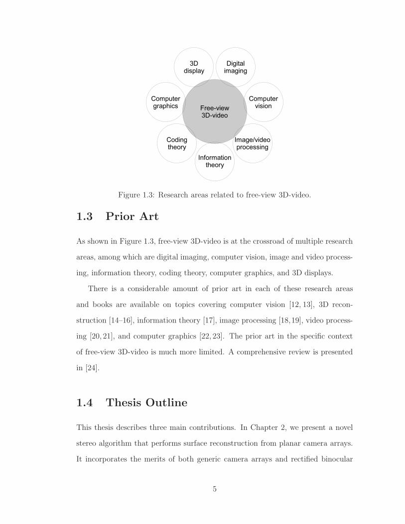
Figure 1.3: Research areas related to free-view 3D-video.

1.3 Prior Art

As shown in Figure 1.3, free-view 3D-video is at the crossroad of multiple research

areas, among which are digital imaging, computer vision, image and video process-

ing, information theory, coding theory, computer graphics, and 3D displays.

There is a considerable amount of prior art in each of these research areas

and books are available on topics covering computer vision [12, 13], 3D recon-

struction [14–16], information theory [17], image processing [18,19], video process-

ing [20, 21], and computer graphics [22, 23]. The prior art in the specific context

of free-view 3D-video is much more limited. A comprehensive review is presented

in [24].

1.4 Thesis Outline

This thesis describes three main contributions. In Chapter 2, we present a novel

stereo algorithm that performs surface reconstruction from planar camera arrays.

It incorporates the merits of both generic camera arrays and rectified binocular

5

setups, recovering large surfaces like the former and performing efficient computa-

tions like the latter. First, we introduce a rectification algorithm which gives free-

dom in the design of camera arrays and simplifies photometric and geometric com-

putations. We then define a novel set of data-fusion functions over 4-neighborhoods

of cameras, which treat all cameras symmetrically and enable standard binocular

stereo algorithms to handle arrays with an arbitrary number of cameras. In par-

ticular, we introduce a photometric fusion function that handles partial visibility

and extracts depth information along both horizontal and vertical baselines. Fi-

nally, we show that layered depth images and sprites with depth can be efficiently

extracted from the rectified 3D space. Experimental results on real images confirm

the effectiveness of the proposed method, which reconstructs dense surfaces 20%

larger than classical stereo methods on Tsukuba.

In Chapter 3, we propose a wavelet-based codec for the static depth-image-

based representation (DIBR), which allows viewers to freely choose the viewpoint.

The proposed codec jointly estimates and encodes the unknown depth map from

multiple views using a novel rate-distortion (RD) optimization scheme. The rate

constraint reduces the ambiguity of depth estimation by favoring piecewise-smooth

depth maps. The optimization is efficiently solved by a novel dynamic program-

ming along the tree of integer wavelet coefficients. The codec encodes the image

and the depth map jointly to decrease their redundancy and to provide an RD-

optimized bitrate allocation between the two. The codec also offers scalability

both in resolution and in quality. Experiments on real data show the effectiveness

of the proposed codec.

In Chapter 4, we present a novel codec of depth-image-based representations

for free-viewpoint 3D-TV. The proposed codec relies on a shape-adaptive wavelet

transform and an explicit representation of the locations of major depth edges.

Unlike classical wavelet transforms, the shape-adaptive transform generates small

6

wavelet coefficients along depth edges, which greatly reduces the data entropy. The

codec also shares the edge information between the depth map and the image to

reduce their correlation. The wavelet transform is implemented by shape-adaptive

lifting, which enables fast computations and perfect reconstruction. Experimental

results on real data confirm the superiority of the proposed codec, with PSNR gains

of up to 5.46 dB on the depth map and up to 0.19 dB on the image compared to

standard wavelet codecs.

Finally in Chapter 5, we consider the reconstruction, compression, and render-

ing from a unique camera moving in a static 3D environment. In particular, we

address the problem of side information extraction for distributed coding of videos.

Two interpolation methods constrained by the scene geometry, i.e., based either

on block matching along epipolar lines or on 3D mesh fitting, are first developed.

These techniques are based on a sub-pel robust algorithm for matching feature

points between key frames. The robust feature point matching technique leads

to semidense correspondences between pairs of consecutive key frames. However,

the underlying assumption of linear motion leads to misalignments between the

side information and the actual Wyner-Ziv frames, which impacts the RD perfor-

mances of the 3D model-based DVC solution. A feature point tracking technique

is then introduced at the decoder to recover the intermediate camera parameters

and cope with these misalignments problems. This approach, in which the frames

remain encoded separately, leads to significant RD performance gains. The RD

performances are then further improved by allowing limited tracking at the en-

coder. When the tracking is performed at the encoder, tracking statistics also

serve as criteria for the encoder to adapt the key frame frequency to the video

motion content.

7

CHAPTER 2

SYMMETRIC STEREORECONSTRUCTION FROMPLANAR CAMERA ARRAYS

2.1 Introduction

Online metaverses have emerged as a way to bring an immersive and interactive

3D experience to a worldwide audience. However, the fully automatic creation

of realistic content for these metaverses is still an open problem. The challenge

here is to achieve simultaneously four goals. First, the rendering quality must be

high for the virtual world to look realistic. Second, the geometric quality must

be sufficient to let physics-based simulation provide credible interactions between

objects. Third, the computational complexity must be simple enough to enable

real-time rendering. Finally, the data must admit a compact representation to

allow data streaming across networks.

In this chapter, we propose three contributions toward these goals. First, we

introduce a special rectified 3D space and an associated rectification algorithm

that handles planar arrays of cameras. It gives freedom in the design of camera

arrays, so that their fields of view can be adapted to the scene being recorded. At

the same time, rectification simplifies the reconstruction problem by making the

coordinates of voxels and their pixel projection integers. This removes the need for

further data resampling and simplifies changes of coordinate systems and visibility

computations.

Second, we present a set of data-fusion functions that enable standard binocular

stereo reconstruction [25] to handle arrays with arbitrary number of cameras. Using

8

one depth map per camera, the algorithm reconstructs large surfaces, up to 20%

larger on Tsukuba, and therefore reduces the holes in novel-view synthesis. We

introduce two Markov random fields (MRF), a classical one over the arrays of pixels

and a novel one over the array of cameras. The latter lets us treat all the cameras

symmetrically by defining fusion functions over 4-neighborhoods of cameras.

Finally, we introduce a global fusion algorithm that merges the depth maps into

a unique layered depth image (LDI) [26], a rich but compact data representation

made of a dense depth map with multiple values per pixel. We also show that the

recovered LDI can be segmented fully automatically into sprites with depth [26].

Such sprites are related to geometry images, which can be efficiently rendered and

compressed [27].

The remainder of the chapter is organized as follows. Section 2.2 presents the

previous work, while Section 2.3 describes the rectified space and the rectifica-

tion homographies. Section 2.4 follows with the proposed stereo reconstruction

algorithm, and Section 2.5 with the creation of a global surface model. Finally,

Section 2.6 presents the experimental results.

2.2 Relation to Previous Work

Surface reconstruction methods fall into two categories, those based on large

generic camera arrays and those based on small rectified stereo setups, most of-

ten binocular, where the optical camera axes are normal to the baseline. The

former [28, 29] handle rich depth information and can reconstruct large surfaces.

However, the genericity of the camera locations makes visibility computations dif-

ficult and voxel projections computationally expensive.

In rectified stereo setups [25, 30, 31], on the other hand, visibility and projec-

tions are simple. These setups also allow efficient reconstruction algorithms based

9

on maximum a-posteriori (MAP) inference over MRFs. However, the depth in-

formation extracted from the images tends to be quite poor, especially for linear

arrays which only take advantage of textures with significant gradients along their

baseline. Moreover, the small number of cameras and the constrained viewing

direction strongly limits the volume inside which depth triangulation is possible.

The constraint on the viewing direction can be removed using rectification,

which trades view freedom for image distortion. So far, however, rectification has

been limited to small stereo setups with two [32, 33] or three [34, 35] cameras.

In this chapter, we introduce a special rectified 3D space and show that when

the problem is defined in terms of transformations between 3D spaces, instead of

alignment of epipolar lines, rectification can be generalized to planar arrays with

arbitrary number of cameras.

Camera arrays have access to much richer information than binocular setups.

Quite surprisingly, however, the extra information can prove to be detrimental and

actually reduce the quality of reconstructed surfaces [36]. The issue comes from

partially visible voxels, whose number increases with the number of cameras. A

number of methods tackle this issue [36–38]. However, most of them are asym-

metric, choosing one camera as a reference. Cameras far apart tend to have less

visible surfaces in common, which limits the number of cameras in the array and,

as a consequence, the area of reconstructed surfaces. Moreover, many multiview

stereo methods disregard the relative locations of the cameras when extracting the

depth information from images [28,39], which reduces the discriminative power of

the extracted information.

In the proposed method, we rely on multiple depth maps, one per camera, and

treat all the cameras symmetrically. Furthermore, we define a novel MRF over

the camera array and take into account the relative locations of the cameras. This

10

way, the proposed method handles arrays with arbitrary number of cameras and

extracts the depth information along both horizontal and vertical baselines.

Surface reconstruction based on multiple depth maps has already been studied

in [39–41] but these methods lacked the proposed rectified 3D space, which led to

costly operations to compute visibility, enforce intercamera geometric consistency,

and merge depth maps.

The proposed extraction of sprites from LDIs is related to depth map segmenta-

tion [42], with the added complexity of multiple depth values per pixel. Moreover,

unlike [43], the segmentation is performed automatically and is not limited to

planar surfaces.

2.3 The Rectified Space

2.3.1 Overview

We first consider the problem of rectifying the 3D space and the 2D camera im-

ages to simplify the stereo reconstruction problem. In the following, points are

represented in homogeneous vectors, with x , (x, y, 1)⊺ denoting a point on the

2D image plane and X , (x, y, z, 1)⊺ a point in 3D space. Points are defined up to

scale: x and λx are equivalent for any nonnull scalar λ. This relation is denoted

by the symbol ‘∼’.

Under the pin-hole camera model [33], a 3D point X and its projection x onto

an image plane are related by

x ∼ PX (2.1)

where P is a 3× 4 matrix which can be decomposed as

P = KR

(

I −c

)

(2.2)

11

where I is the identity matrix, R the camera rotation matrix, c the optical center,

and K the matrix of intrinsic parameters. All these parameters are assumed known.

The optical centers of the cameras are assumed to lie on a planar lattice, that

is,

c = o + mv1 + nv2 (2.3)

where o is the center of the grid, v1 and v2 are two noncollinear vectors, and m

and n are two signed integers. The classical stereo pair is a special case of such

an array. Since a pair (m, n) uniquely identifies a camera, we use it to index the

cameras and denote by C the set of pairs (m, n).

The proposed rectification consists in rotating the cameras and transforming

the Euclidean 3D space using homographies. The rectified 3D space is defined as

a space where the projection matrices P(m,n) take the special form

P(m,n) =

1 0 −m 0

0 1 −n 0

0 0 0 1

. (2.4)

It follows that, in the rectified space, a 3D point X = (x, y, d, 1)⊺ is related to

its 2D projection x(m,n) =(

x(m,n), y(m,n), 1)⊺

on the image plane of camera (m, n)

by the equations

x(m,n) = x−md,

y(m,n) = y − nd.

(2.5)

The 2D motion vectors of image points from camera (m, n) to camera (m′, n′)

are equal to d times the baseline (m−m′, n−n′)⊺. Therefore, the third coordinate d

of the rectified 3D space is a disparity, while the third coordinate z of the Euclidean

space is a depth.

The projection of an integer-valued point X is also an integer. Moreover, the

12

Figure 2.1: A few rays of light in the rectified 3D space: rays passing through theoptical centers of camera (0, 0) (a) and camera (1, 0) (b). The rays are alignedwith the voxel grid, which simplifies visibility computations.

rays of light passing through the optical centers are parallel to one another and

fall on integer-valued 3D points, as shown in Figure 2.1, which simplifies visibility

computations.

2.3.2 Rectification homographies

First, we need to recover the grid parameters o, v1, and v2 from the projection

matrices P(m,n). From (2.3), we obtain the system of equations

(

I mI nI

)

o

v1

v2

= c(m,n), ∀(m, n) ∈ C. (2.6)

In the general case, this system is over-constrained and the vectors are obtained

by least mean-square. When the cameras are collinear, one of the vectors is free

to take any value. In that case, the constrained vector is computed by least mean-

square and the free vector is chosen to limit the image distortion. To do so, the

normal vector defined by the cross-product v1 ∧ v2 is set to the mean of the unit

vectors on the optical axes. The free vector is then deduced by Gram-Schmidt

orthogonalization.

We define an intrinsic-parameter matrix K shared by all the rectified cameras

13

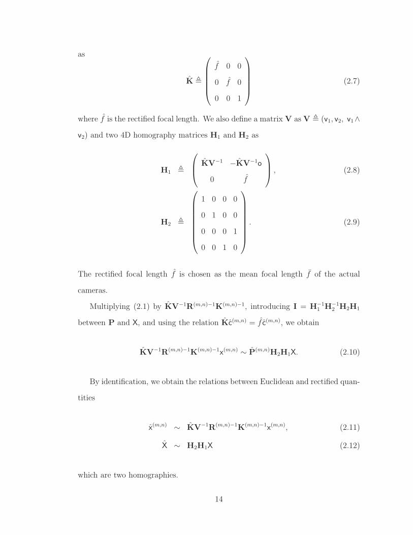
as

K ,

f 0 0

0 f 0

0 0 1

(2.7)

where f is the rectified focal length. We also define a matrix V as V , (v1, v2, v1∧

v2) and two 4D homography matrices H1 and H2 as

H1 ,

KV−1 −KV−1o

0 f

, (2.8)

H2 ,

1 0 0 0

0 1 0 0

0 0 0 1

0 0 1 0

. (2.9)

The rectified focal length f is chosen as the mean focal length f of the actual

cameras.

Multiplying (2.1) by KV−1R(m,n)−1K(m,n)−1, introducing I = H−11 H−1

2 H2H1

between P and X, and using the relation Kc(m,n) = f c(m,n), we obtain

KV−1R(m,n)−1K(m,n)−1x(m,n) ∼ P(m,n)H2H1X. (2.10)

By identification, we obtain the relations between Euclidean and rectified quan-

tities

x(m,n) ∼ KV−1R(m,n)−1K(m,n)−1x(m,n), (2.11)

X ∼ H2H1X (2.12)

which are two homographies.

14

The reconstruction of surfaces in the Euclidean space via depth estimation

in the rectified space is then a three-step process. First, images are rectified by

applying the homography (2.11). Then 3D points are estimated in the rectified

space by matching the rectified images. Finally, these 3D points are transfered

back to the Euclidean space by inverting the homography (2.12). Figure 2.2 shows

an example of rectified images.

2.4 Stereo Reconstruction

2.4.1 Overview

We now turn to the stereo reconstruction. In this section, we assume that the

images have been rectified and we drop the hat over mathematical symbols in the

rectified space.

In order to reduce the computational complexity, the dependencies between

cameras in the array are modeled using a MRF where each camera (m, n) is asso-

ciated with an image I(m,n) and a disparity map D(m,n), as shown in Figure 2.3.

Specifically, each value D(m,n)x,y represents the disparity of a 3D point along the ray

of light passing by pixel (x, y) in camera (m, n). At each camera, the dependencies

between pixels are also modeled using a MRF. Stereo reconstruction then aims at

inferring the hidden disparity maps from the observed images, relations between

occupancy and visibility, unicity of the reconstructed scene, and the Markov priors.

An approximate solution is obtained by an iterative process, at the heart of

which lie classical MAP-MRF inferences [30,31,41] applied independently on each

camera. Each inference aims at solving an optimization of the form

minD

∑

(x,y)∈P

(

Px,y,Dx,y+ λgGx,y,Dx,y

+ Sx,y(D))

(2.13)

15

(a) Original images

(b) Rectified images

Figure 2.2: Rectification of four images from the toy sequence [44]. After rectifi-cation, both the rows and the columns of the images are aligned.

I(−1,0)

D(−1,0)

I(0,0)

D(0,0)

I(1,0)

D(1,0)

I(2,0)

D(2,0)

I(−1,1)

D(−1,1)

I(0,1)

D(0,1)

I(1,1)

D(1,1)

I(2,1)

D(2,1)

Figure 2.3: Camera MRF associated with a 2× 4 camera array. Each node repre-sents a camera with an observed image I and a hidden disparity map D. Edgesrepresent fusion functions.

16

where P denotes the set of 2D pixels, λg is a scalar weight, S is a clique po-

tential favoring piecewise-smoothness [30], and Px,y,d and Gx,y,d are respectively

photometric and geometric cost volumes.

The proposed algorithm alternates between inferences and cost volume com-

putations. Its novelty lies in the set of fusion functions computing the costs vol-

umes. Due to the Markov assumption, the fusion functions are defined over 4-

neighborhoods N4, i.e., cross-shaped groups of five cameras, which usually contain

rich depth information but only limited partial occlusions. The overall complexity

of the proposed algorithm is linear in the size of the data.

Although limited, partial occlusions tend to create large photometric costs at

voxels on the surfaces, which leads to erroneous disparities. These outlier costs can

be removed by an explicit visibility modeling [38]. However, visibility depends on

the surface geometry, which introduces a circular dependency. We solve this issue

by introducing an implicit model of partial occlusions, which does not depend on

the surface geometry.

Robust statistics over the four pairwise cliques of each camera 4-neighborhood

can reduce the impact of outlier costs. However, classical robust statistics do not

take into account the relative locations of the cameras and may fail to extract

the depth information along both horizontal and vertical baselines, leading to

photometric cost volumes with poor discriminative power.

Therefore, we propose a robust measure which strives to include the photo-

metric costs from at least one vertical and one horizontal camera clique at each

voxel. We do this by introducing an assumption we call “visibility by opposite

neighbors”: a voxel visible by a camera (m, n) is also visible by at least one of

its horizontal camera neighbors (m − 1, n) and (m + 1, n), and by at least one of

its vertical camera neighbors (m, n − 1) and (m, n + 1). This assumption usually

holds, except for instance for surfaces like picket fences or cameras having less than

17

four neighbors. In the following, we denote the quantities related to horizontal and

vertical pairwise cliques by the superscripts h and v, respectively.

2.4.2 Geometric cost volume G(m,n)

The geometric cost volumes G(m,n) favor consistent disparity maps. In order to

compute them, the disparity maps D(m,n)x,y are first transformed into binary occu-

pancy volumes δ(m,n)x,y,d , whose voxels take value one when they contain surfaces. An

occupancy volume δ(m,n)x,y,d is obtained by initializing it to zero, except at the set of

voxels {(x, y,D(m,n)x,y )} where it is initialized to one.

Since all the occupancy volumes represent the same surfaces, they should be

identical up to visibility and a change of coordinate system. Thanks to the rectifi-

cation leading to (2.5), changing the coordinate system of a volume δ from camera

(0, 0) to camera (m, n) is simply an integer 3D shear φ(m,n) given by

φ(m,n)x,y,d (δ) = δx+md,y+nd,d. (2.14)

A change of coordinate system between two arbitrary cameras is obtained by con-

catenating two 3D shears.

Let us consider camera (m, n) and shear the occupancy volumes of its 4-

neighbors to its coordinate system. Using the assumption of visibility by opposite

neighbors, erroneous occupancy voxels are removed using

δ(m,n)x,y,d ← δ

(m,n)x,y,d ∧

(

δ(m+1,n)x,y,d ∨ δ

(m−1,n)x,y,d

)

∧(

δ(m,n+1)x,y,d ∨ δ

(m,n−1)x,y,d

)

(2.15)

where ∨ and ∧ denotes respectively the “or” and “and” operators.

18

The geometric cost volume is then computed as

G(m,n)x,y,d ←

0, if δ(m,n)x,y,d′ = 0, ∀d′

minδ(m,n)

x,y,d′6=0

min (|d− d′| , τ1) , otherwise(2.16)

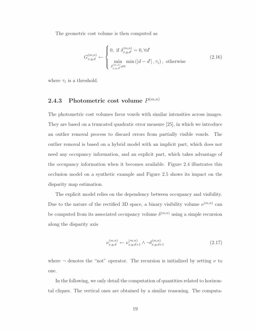
where τ1 is a threshold.

2.4.3 Photometric cost volume P (m,n)

The photometric cost volumes favor voxels with similar intensities across images.

They are based on a truncated quadratic error measure [25], in which we introduce

an outlier removal process to discard errors from partially visible voxels. The

outlier removal is based on a hybrid model with an implicit part, which does not

need any occupancy information, and an explicit part, which takes advantage of

the occupancy information when it becomes available. Figure 2.4 illustrates this

occlusion model on a synthetic example and Figure 2.5 shows its impact on the

disparity map estimation.

The explicit model relies on the dependency between occupancy and visibility.

Due to the nature of the rectified 3D space, a binary visibility volume ν(m,n) can

be computed from its associated occupancy volume δ(m,n) using a simple recursion

along the disparity axis

ν(m,n)x,y,d ← ν

(m,n)x,y,d+1 ∧ ¬δ

(m,n)x,y,d+1 (2.17)

where ¬ denotes the “not” operator. The recursion is initialized by setting ν to

one.

In the following, we only detail the computation of quantities related to horizon-

tal cliques. The vertical ones are obtained by a similar reasoning. The computa-

19

(a) Three images of two fronto-parallelplanes: a dark square in front of a brightbackground.

(b) Photometric cost at iteration 1: theimplicit model removes partial occlusionsin camera 1 and limits their impact incameras 0 and 2.

(c) Photometric cost at iteration 2: theexplicit model removes partial occlusionsin all the cameras.

(d) Disparity maps at iteration 1: errorsremain on cameras 0 and 2.

(e) Disparity maps at iteration 2: no errorremains.

Figure 2.4: A simple example demonstrating the behavior of the occlusion model.Perfect disparity maps are obtained in two iterations.

(a) Truncated quadratic cost (b) Proposed cost

Figure 2.5: Cropped disparity maps computed on Tsukuba with five cameras form-ing a cross. The proposed photometric cost reduces the disparity errors due topartial occlusions.

20

tions are conducted independently at each voxel, so we drop the subscript (x, y, d).

We define I(m,n) as the intensity volume obtained by replicating the image I(m,n)

along the disparity axis.

Let us consider the camera (m, n) and its 4-neighborhood. Using (2.14), the

intensity and visibility volumes are sheared to the coordinate system of camera

(m, n). From the truncated quadratic error model and the assumption of visibility

by opposite neighbors, an horizontal error volume Eh(m,n) is computed as

Eh(m,n) = min(

(

I(m,n) − I(m−1,n))2

,

(

I(m,n) − I(m+1,n))2

, τ2

)

(2.18)

where τ2 is a threshold.

The photometric cost Eh(m,n) may still contain large values when the assump-

tion of visibility by opposite neighbors is violated. Therefore, we further discard

outliers by explicitly computing visibility. Using De Morgan’s laws, the validity of

the costs is computed as

V h(m,n) = ¬ν(m,n) ∨ ν(m−1,n) ∨ ν(m+1,n). (2.19)

We now have two pairs of error and validity volumes, (Eh(m,n), V h(m,n)) hor-

izontally and (Ev(m,n), V v(m,n)) vertically. In order to create a photometric cost

volume which includes the depth information from both vertical and horizontal

texture gradients, we define this cost volume as the weighted average

P (m,n) =V h(m,n)Eh(m,n) + V v(m,n)Ev(m,n)

V h(m,n) + V v(m,n), (2.20)

which is only defined when at least one of the validity volumes takes a nonzero

value. Values at voxels where this is not the case are obtained by interpolation.

21

(a) Texture

(b) Disparity

Figure 2.6: The 3-layer LDI obtained on Tsukuba with 25 cameras. By treatingall the cameras symmetrically, the proposed algorithm recovers large areas, whichmay be occluded in the central camera.

2.5 Global Surface Representation

2.5.1 Layered depth image

Using the special nature of the 3D rectified space, we present a simple and efficient

procedure to merge the multiple disparity maps into a unique LDI [26]. The LDI

offers a compact and global surface representation. Figure 2.6 shows an example

of LDI.

To begin with, the disparity maps D(m,n) are transformed into occupancy vol-

umes δ(m,n) as detailed in Section 2.4.2. These volumes are then sheared to a

reference coordinate system, the one of camera (0, 0) for instance.

The disparity layers are extracted in a front to back order by voting. Visibility

22

volumes ν(m,n) are computed from their associated occupancy volumes using (2.17)

and an aggregation volume A is obtained using

Ax,y,d =∑

(m,n)∈C

ν(m,n)x,y,d δ

(m,n)x,y,d . (2.21)

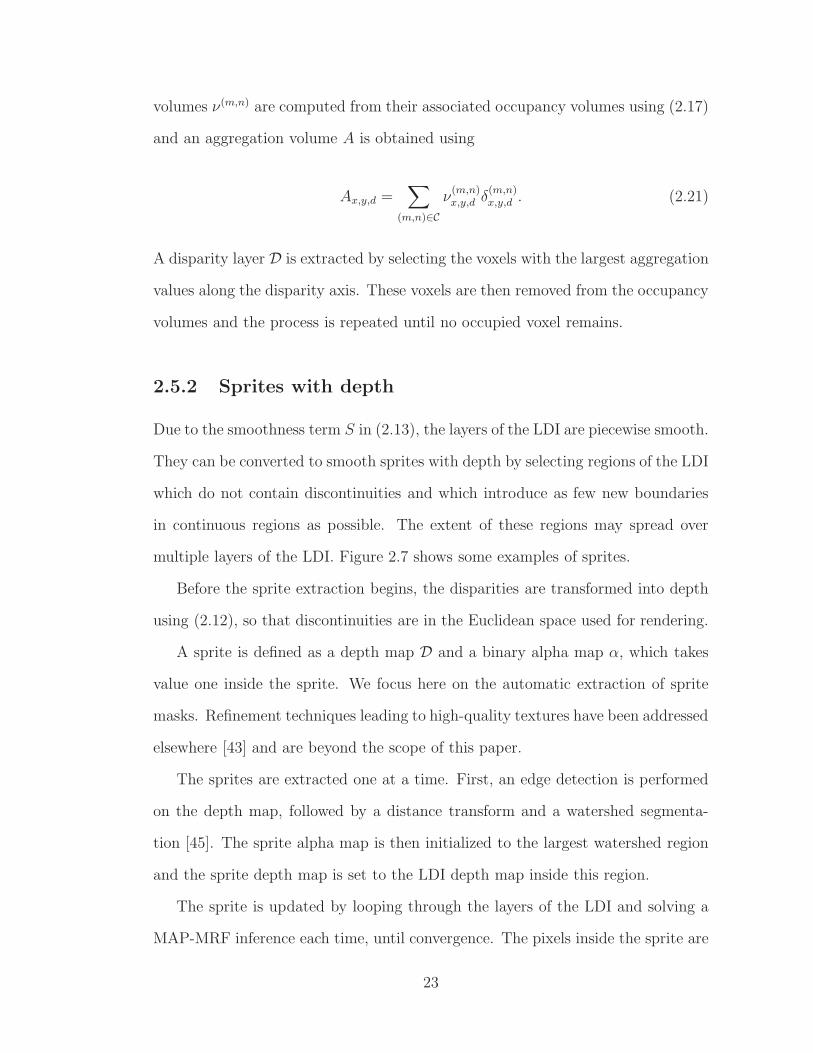
A disparity layer D is extracted by selecting the voxels with the largest aggregation

values along the disparity axis. These voxels are then removed from the occupancy

volumes and the process is repeated until no occupied voxel remains.

2.5.2 Sprites with depth

Due to the smoothness term S in (2.13), the layers of the LDI are piecewise smooth.

They can be converted to smooth sprites with depth by selecting regions of the LDI

which do not contain discontinuities and which introduce as few new boundaries

in continuous regions as possible. The extent of these regions may spread over

multiple layers of the LDI. Figure 2.7 shows some examples of sprites.

Before the sprite extraction begins, the disparities are transformed into depth

using (2.12), so that discontinuities are in the Euclidean space used for rendering.

A sprite is defined as a depth map D and a binary alpha map α, which takes

value one inside the sprite. We focus here on the automatic extraction of sprite

masks. Refinement techniques leading to high-quality textures have been addressed

elsewhere [43] and are beyond the scope of this paper.

The sprites are extracted one at a time. First, an edge detection is performed

on the depth map, followed by a distance transform and a watershed segmenta-

tion [45]. The sprite alpha map is then initialized to the largest watershed region

and the sprite depth map is set to the LDI depth map inside this region.

The sprite is updated by looping through the layers of the LDI and solving a

MAP-MRF inference each time, until convergence. The pixels inside the sprite are

23

Figure 2.7: Examples of sprites extracted from the LDI of Tsukuba with 25 cam-eras. Note the absence of occlusion on the cans.

then removed from the LDI, the newly visible pixels moved to the first layer, and

the process repeated.

The MAP-MRF inference proceeds as follows. Let D(LDI) and α(LDI) be re-

spectively the depth map and the binary alpha map of the current LDI layer. The

sprite and the LDI layer are first fused together to form D and α such that

αx,y = αx,y ∨ α(LDI)x,y ,

Dx,y = αx,yDx,y + (1− αx,y)D(LDI)x,y .

(2.22)

At each pixel (x, y), we define a likelihood px,y of belonging to the sprite and

we model its dependencies by a MRF. The likelihoods inside the sprite mask are

fixed to one and three transition functions are defined

px′,y′ =

(1− 2ρ0)px,y + ρ0 where smooth,

(1− 2ρ1)px,y + ρ1 at small depth differences,

min (1− px,y, 1/2) at discontinuities,

where ρ0 and ρ1 are two transition likelihoods with 0 ≤ ρ0 < ρ1 ≤ 1/2. The third

transition function states that at a discontinuity� if one side belongs to the sprite, the other one does not,

24

Figure 2.8: Disparity map obtained from the four rectified images of the toy se-quence shown in Figure 2.2.� if one side does not belong to the sprite, there is no constraint on the other

side.

Once the inference has been solved, the sprite alpha map is set to one where p is

greater than 1/2 and the sprite depth map is updated accordingly.

2.6 Experimental Results

First, the rectification and stereo reconstruction algorithms are validated on four

images from the toy sequence [44]. The four cameras form a 2 × 2 array with

nonparallel optical axes and nonsquare cells. Figure 2.2 shows the output of the

rectification algorithm. Rectification aligns the rows and columns of the images

and introduces a limited amount of distortion. Figure 2.8 shows the disparity map

obtained by the proposed stereo reconstruction algorithm after five iterations. The

geometry of the scene appears clearly.

The stereo reconstruction is then tested on the binocular sequences of the Mid-

dlebury dataset [25]. In this case, the configuration of the cameras is such that

rectification does not introduce any image distortion. Figure 2.9 shows the dispar-

ity maps obtained by the proposed method using fixed parameters. The proposed

25

Figure 2.9: Disparity maps obtained on the Middlebury dataset with two cameras.The occlusion model leads to sharp and accurate depth discontinuities.

method performs consistently well over the set of sequences. In particular, it does

not suffer from foreground fattening [25]: occlusion modeling, geometric consis-

tency, and piecewise smoothness lead to disparity maps with discontinuities which

are both sharp and accurately located. The disparity maps contain few errors,

mostly located on the left and right image borders, where less depth information

is available.

Since the ground truth is known for this dataset, we also present numerical

performance results in Table 2.1. The error rates of the proposed method are close

to those of the best binocular methods.

Unlike binocular methods, however, the proposed method scales with the num-

ber of cameras. Table 2.2 presents the error rates of the proposed algorithm and

26

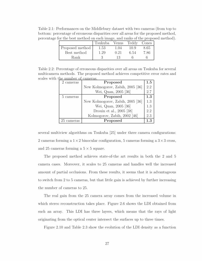
Table 2.1: Performances on the Middlebury dataset with two cameras (from top tobottom: percentage of erroneous disparities over all areas for the proposed method,percentage for the best method on each image, and ranks of the proposed method).

Tsukuba Venus Teddy ConesProposed method 1.53 1.04 10.9 8.65

Best method 1.29 0.21 6.54 7.86Rank 3 13 6 6

Table 2.2: Percentage of erroneous disparities over all areas on Tsukuba for severalmulticamera methods. The proposed method achieves competitive error rates andscales with the number of cameras.

2 cameras Proposed 1.5New Kolmogorov, Zabih, 2005 [36] 2.2

Wei, Quan, 2005 [36] 2.75 cameras Proposed 1.3

New Kolmogorov, Zabih, 2005 [36] 1.3Wei, Quan, 2005 [36] 1.3

Drouin et al., 2005 [38] 2.2Kolmogorov, Zabih, 2002 [46] 2.3

25 cameras Proposed 1.3

several multiview algorithms on Tsukuba [25] under three camera configurations:

2 cameras forming a 1×2 binocular configuration, 5 cameras forming a 3×3 cross,

and 25 cameras forming a 5× 5 square.

The proposed method achieves state-of-the art results in both the 2 and 5

camera cases. Moreover, it scales to 25 cameras and handles well the increased

amount of partial occlusions. From these results, it seems that it is advantageous

to switch from 2 to 5 cameras, but that little gain is achieved by further increasing

the number of cameras to 25.

The real gain from the 25 camera array comes from the increased volume in

which stereo reconstruction takes place. Figure 2.6 shows the LDI obtained from

such an array. This LDI has three layers, which means that the rays of light

originating from the optical center intersect the surfaces up to three times.

Figure 2.10 and Table 2.3 show the evolution of the LDI density as a function

27

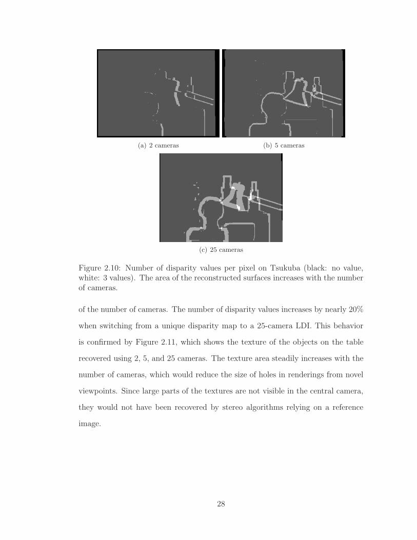
(a) 2 cameras (b) 5 cameras

(c) 25 cameras

Figure 2.10: Number of disparity values per pixel on Tsukuba (black: no value,white: 3 values). The area of the reconstructed surfaces increases with the numberof cameras.

of the number of cameras. The number of disparity values increases by nearly 20%

when switching from a unique disparity map to a 25-camera LDI. This behavior

is confirmed by Figure 2.11, which shows the texture of the objects on the table

recovered using 2, 5, and 25 cameras. The texture area steadily increases with the

number of cameras, which would reduce the size of holes in renderings from novel

viewpoints. Since large parts of the textures are not visible in the central camera,

they would not have been recovered by stereo algorithms relying on a reference

image.

28

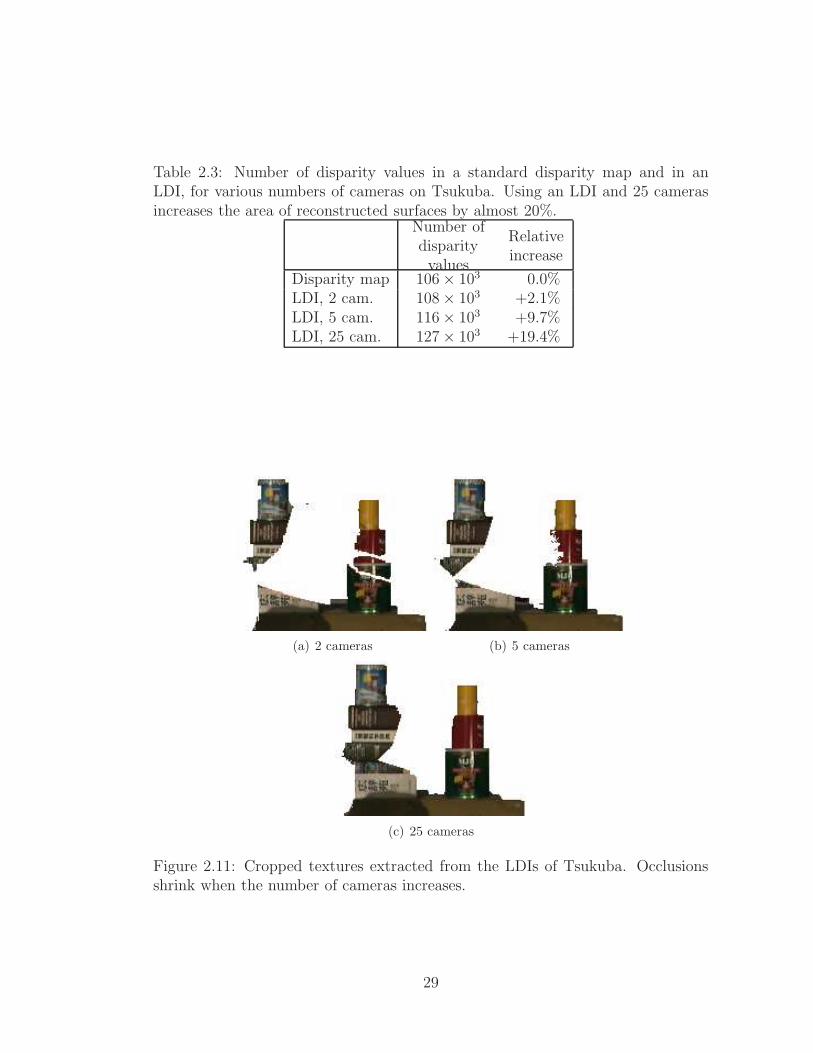
Table 2.3: Number of disparity values in a standard disparity map and in anLDI, for various numbers of cameras on Tsukuba. Using an LDI and 25 camerasincreases the area of reconstructed surfaces by almost 20%.

Number ofdisparityvalues

Relativeincrease

Disparity map 106× 103 0.0%LDI, 2 cam. 108× 103 +2.1%LDI, 5 cam. 116× 103 +9.7%LDI, 25 cam. 127× 103 +19.4%

(a) 2 cameras (b) 5 cameras

(c) 25 cameras

Figure 2.11: Cropped textures extracted from the LDIs of Tsukuba. Occlusionsshrink when the number of cameras increases.

29

2.7 Conclusion

In this chapter, we have first presented a novel rectification algorithm that han-

dles planar camera arrays of any size and greatly simplifies the reconstruction of

3D surfaces. Second, we have introduced a stereo reconstruction method that

treats all cameras symmetrically and scales with the number of cameras. Finally,

we have presented novel algorithms to merge the estimated disparity maps into

layered depth images and sprites with depth. We have validated the proposed

methods by experimental results on arrays with various camera configurations and

reconstructed dense surfaces 20% larger than classical stereo methods on Tsukuba.

Future work will consider multiple planar arrays to obtain closed surfaces.

30

CHAPTER 3

WAVELET-BASED JOINTESTIMATION ANDENCODING OF DIBR

3.1 Introduction

Free-viewpoint three-dimensional television (3D-TV) aims at providing an en-

hanced viewing experience not only by letting viewers perceive the third spatial

dimension via stereoscopy but also by allowing them to move inside the 3D video

and freely choose the viewing location they prefer [47]. The free-viewpoint ap-

proach is also useful for multiuser autostereoscopic 3D displays [48], which have to

generate a large number of viewpoints.

The fundamental problem posed by 3D-TV lies in the massive amount of data

required to represent the set of all possible views or, equivalently, the set of all light

rays in the scene. This set of light rays, called the plenoptic function [11], lies in

general in a seven-dimensional space. Each light ray travels along a line, which is

described by a point (three dimensions), an angular orientation (two dimensions),

and a time instant (one dimension). The last dimension describes the spectrum,

or color, of the light rays. By comparison, 2D videos only lie in a four-dimensional

space made of two angles, time, and color. Therefore, 3D-TV requires the design

of a novel video chain [47].

A large number of methods have been proposed to record and encode the

plenoptic function [49]. They widely differ in the amount of 3D geometry used

to encode the data, which ranges from no geometry at all (e.g., light field) to an

extremely accurate geometry (e.g., texture mapping). On the one hand, relying on

31

the geometry has the advantage of requiring fewer cameras to record the plenoptic

function and allowing the reduction of redundancies between the recorded views [9,

50]. On the other hand, using the geometry has the drawback of limiting the

realism of the synthesized views and requiring a difficult estimation of the 3D

geometry. Indeed, passive 3D geometry estimation from multiple views suffers

from ambiguities, while estimation based on active lighting has only a narrow

scope of application [47].

An efficient trade-off on the 3D geometry, called the depth-image-based rep-

resentation (DIBR), consists in approximating the plenoptic function using pairs

of images and depth maps [8]. Now part of the MPEG-4 standard [10, 51], this

representation allows arbitrary views to be rendered in the vicinity of these pairs.

Since depth maps tend to have lower entropies than images, the DIBR leads to

compact bitstreams. Moreover, realistic images can be synthesized from the DIBR

using image-based rendering (IBR) and depth maps do not need to be estimated

extremely accurately, as long as the viewpoint does not change too much.

Encoding the DIBR presents two difficulties. First, the depth maps are un-

known. Therefore, not only do they have to be encoded, but they also have to

be estimated. Second, the relation between the depth maps and the distortion of

the plenoptic function is highly nonlinear, which makes the rate-distortion (RD)

optimization difficult. In particular, finding an optimal bitrate allocation between

images and depth maps is nontrivial.

A number of methods have avoided these issues by excluding depth maps from

the RD problem. For instance, in [50, 52] depth maps are obtained using block-

based depth estimation, essentially a motion estimation, and encoded in a lossless

fashion. As an alternative to blocks, depth can also be estimated using meshes [53,

54] or pixel-wise regularization [8]. However, in such methods the image encoder

32

and the depth encoder operate at different RD slopes, which penalizes the overall

codec efficiency and makes it difficult to optimally allocate the bitrate [55].

A more principled approach consists in linearizing the RD problem [56,57] using

Taylor series expansions and statistical analysis. It has the advantage of leading to

closed-form expressions and allowing a theoretical analysis of the problem. How-

ever, linearization is only valid for small depth approximations.

Another way of handling the nonlinearity is to assume that depth maps take

a finite number of discrete values. Under some constraints on the dependencies

between depth values, globally optimal solutions can be found using dynamic pro-

gramming [58]. For instance, optimal solutions exist when depth maps are encoded

using differential pulse code modulation (DPCM) [59] or quadtrees [60]. This ap-

proach does not require any ground truth; the estimation and encoding of the depth

maps are carried out jointly. It also takes advantage of the bitrate constraint to

favor smooth depth maps, much as ad-hoc smoothness terms do in computer vi-

sion [25], which reduces the ambiguity of the estimation.

In this chapter, we propose a new wavelet-based DIBR codec which performs

an RD-optimized encoding of multiple views. It differs from classical wavelet-based

codecs in that part of the data to be transformed (i.e., the depth map) is unknown.

Here, as shown in Figure 3.1, both the depth estimation and the depth and image

encoding are performed jointly. Although the problem is nonlinear, we present a

codec able to efficiently find optimal solutions without resort to linearization. We

show that when the depth maps are represented using special integer wavelets,

their joint estimation and coding via RD-optimization can be efficiently solved us-

ing dynamic programming (DP) along the tree of wavelet coefficients. The DP we

introduce in this chapter differs from that of quadtrees [61], as discussed in Sec-

tion 3.3.4. The RD-optimization of the integer wavelets favors piecewise-smooth

depth maps, which reduces the estimation ambiguity and leads to compact repre-

33

Figure 3.1: Overview of the proposed codec: the encoder takes multiple views andjointly estimates and encodes a depth map together with a reference image (theDIBR). The output DIBR can be used to render free viewpoints.

sentations of the data. The joint encoding of the images and depth maps provides

an RD-optimized bitrate allocation. Furthermore, using the fact that depth dis-

continuities usually happen at image edges, it reduces the redundancies between

depth maps and images by coding the two wavelet significance maps only once.

In addition, the proposed codec offers scalability both in resolution, using

wavelets, and in quality, using quality layers. The former allows servers to ef-

ficiently stream data to display devices with inhomogeneous display resolutions

and inside online virtual 3D worlds, where the DIBR may actually only cover a

small portion of the display due to its distance to the viewpoint. The latter lets

servers efficiently stream data over networks with inhomogeneous capabilities. In

both cases, the RD point is chosen on the fly at the server by truncating the

bitstream [19].

There is a close relation between depth maps and 2D motion fields: depth

maps define 3D surfaces, whose projection onto image planes gives rise to motion

fields. Therefore, the techniques designed to solve the RD problem of classical 2D

video coding [62] can usually also be applied to DIBR. Among these techniques,

those described in [63, 64] are related to the proposed wavelet-based coding. In

these codecs, images are split into blocks of variable sizes using quadtrees, and the

motion vectors are DPCM coded. Like our codec, they achieve global optimality

34

using dynamic programming. However, besides being not scalable, their complexity

is exponential in the block sizes, which limits the range of block sizes they can

handle. The complexity of our proposed codec is only linear in the number of

wavelet decomposition levels, due to the special tree structure we introduce.

The remainder of the chapter is organized as follows. Section 3.2 presents

the RD problem at hand, while Section 3.3 details the optimization of the DIBR.

Finally, Section 3.4 presents our experimental results.

3.2 Problem Formulation

First, we define the RD problem that will be solved by the proposed codec. As

illustrated in Figure 3.1, the encoder takes a set of synchronized views as input and

represents them using the DIBR. The decoder receives the DIBR and synthesizes

novel views at 3D locations chosen by the viewers.

The DIBR consists in a subset of the views, called reference views, along

with unknown depth maps. In the following, we limit our study to the case of

static grayscale views. In this case, the DIBR provides an approximation to five-

dimensional plenoptic functions with three spatial dimensions and two angular

dimensions. Since the DIBR only offers a local approximation of the plenoptic

function, the viewers are free to choose arbitrary viewpoints, but only inside a

region of interest (ROI). A natural choice for the shape of the ROI is to take the

union of a set of hypervolumes made of 3D spheres in space and 2D discs in angle,

with one hypervolume associated to each pair of image and depth map. Since the

approximation does not usually degrade abruptly when the distance increases, the

decoder could actually enforce a “soft” ROI boundary by discouraging the viewer

from choosing a viewpoint outside of the ROI without forbidding it.

The distortion introduced by the codec is measured using the mean-square

35

error (MSE) between the recorded views and the views rendered from the DIBR.

Denoting the vth recorded view and its rendered counterpart respectively by the

column vectors Iv and Iv obtained by stacking all the pixels together, the distortion

can be written as

1

NmNnNv

Nv−1∑

v=0

∥

∥

∥Iv − Iv

∥

∥

∥

2

2(3.1)

where ‖.‖2 denotes the 2-norm, Nm, and Nn are respectively the number of rows and

columns in the views, and Nv is the number of views. We denote by N , NmNnNv

the total number of pixels.

The decoder renders novel views using the nearest pair of image and depth

map. This coding scheme is similar to the encoding Intra (I) and Predictive (P)

in the MPEG standard [62]: reference views are I frames while all the other views

are P frames. The total distortion is then the sum of the distortions associated

with each pair of image and depth map. Likewise, the pairs of images and depth

maps are encoded independently of one another, so that the total bitrate is also

the sum of the bitrates associated with each pair. A differential encoding could

increase the bitrate savings but would at the same time reduce the ability of the

decoder to access views randomly [49].

As a consequence, the RD problem can be solved for each pair of image and

depth map independently. Without loss of generality, the remainder of this article

only considers the case where a unique pair is encoded and the reference view is

indexed by v = 0.

The quantized depth map takes a finite number of discrete values, which define a

set of iso-depth planes, as shown in Figure 3.2. Each plane induces a special motion

field between the reference view and an arbitrary view which is a homography [14],

as shown in Figure 3.3. This class of motion fields has the property of transforming

quadrilaterals into quadrilaterals and includes affine transforms as a special case.

36

Figure 3.2: The spatial extent of a ROI (sphere) with one pair of image anddepth map, along with seven views (cones). The central dark cone designates thereference view. The planes represent iso-depth surfaces (3D model reproducedwith permission from Google 3D Warehouse).

In the particular case of rectified views [14], the motion vectors are parallel to the

baseline of the pair of views.

In this framework, the depth estimation is formulated in terms of disparities,

which are inversely proportional to depths. Disparities are better suited to the

geometry of the problem at hand. They take into account the decreasing accuracy

of the depth estimation as depth increases and they are equal to motion vectors in

the case of rectified views.

Both the reference view and the disparity map are encoded in a lossy manner.

Let us denote the encoded reference view by the vector I0 and the jointly estimated

and encoded disparity map by the vector δ. The view Iv is approximated by forward

motion compensation of the reference view I0 using the estimated disparity map δ,

an operation denoted by Mfv (I0; δ) where the f stands for ‘forward.’

The forward motion compensation is performed using an accumulation buffer

and multiple texture-mapping operations, which benefit from hardware accelera-

tion [65]. The accumulation buffer consists in a memory buffer which is initially

empty and progressively filled by the intensity values of texture-mapped views.

37

(a) A reference view s = 0 along with an arbitrary view s = 1 and an iso-depth plane.

(b) The two views and the associated motion fields.

Figure 3.3: The projection of an iso-depth plane onto two views gives rise to amotion field between the two which is a 2D homography.

38

For each disparity value d, the following three steps are taken:� A binary mask m(δ, d) is defined, which takes value one at pixels with dis-

parity value d.� The homography associated with the disparity value d is applied to both the

reference view I0 and the mask m(δ, d) using texture mapping.� The values of the pixels in the accumulation buffer for which the motion-

compensated mask is one are replaced by those in the motion-compensated

view.

In order to enforce occlusion relations between the iso-depth planes, the dispar-

ities are processed in decreasing depth order. The issues of resampling and hole

filling are solved using bilinear interpolation and texture propagation by Poisson

equation [66].

We shall encode both the image I0 and the disparity map δ in the wavelet

domain. Let c and d be the column vectors of their wavelet coefficients, respectively.

The wavelet synthesis operators relate these vectors by

I0 , Tc and δ , T (d), (3.2)

where the matrix T represents the linear wavelet transform for the image and

the function T represents the integer-to-integer wavelet transform for the discrete-

valued disparity map.

We define two significance maps, σ(c) and σ(d), which are binary vectors with

value one in the presence of nonnull wavelet coefficients and zero otherwise. These

maps are not directional, i.e., they are the same for all directional subbands at

each scale of the 2D wavelet transform. In this way, we will be able to compare

39

σ(c) and σ(d) even when the wavelet operators T and T differ in their directional

division of the frequency plane.

In natural images, discontinuities in the disparity map are usually associated

with discontinuities in the image. When they are not, it is very difficult to estimate

the disparity discontinuities from multiple views. Therefore, we can reduce the data

redundancy of the DIBR by coding the image and the disparity significance maps

jointly. This is done by coding only the significance map of the image σ(c) and

assuming the significant coefficients in σ(d) to be a subset of those in σ(c), that is,

σ(c) = 0⇒ σ(d) = 0. (3.3)

This joint encoding also reduces the complexity of the search for the optimal vector

d∗ by fixing a large number of its coefficients to zero.

The total rate R(c, d) is then given by the sum of the rates R(c) and R(d|σ(c))

and the RD problem is

minc,d

1

N

Nv−1∑

v=0

∥

∥Iv −Mfv(Tc; T (d))

∥

∥

2

2

such that R(c) + R(d|σ(c)) ≤ Rmax

(3.4)

where Rmax is the maximum rate allowed. The constraint σ(c) = 0 ⇒ σ(d) = 0

appears implicitly in the rate constraint: R(d|σ(c)) takes the value +∞ when this

constraint is violated. Introducing the Lagrange multiplier λ [67], (3.4) can be

written as

minc,d

1

N

Nv−1∑

v=0

∥

∥Iv −Mfv(Tc; T (d))

∥

∥

2

2+ λ (R(c) + R(d|σ(c))) . (3.5)

This equation has three goals. First, it encodes the reference view. Second, it

estimates the disparity map, and therefore allows the rendering of arbitrary views.

40

Finally, it encodes this disparity map. Solving this optimization will be the topic

of the next section.

3.3 Rate-Distortion Optimization

3.3.1 Overview

Since (3.5) is nonlinear, solving it is not a trivial operation. Therefore, we formulate

several approximations to obtain a computationally efficient method.

First, we ignore the issues of occlusions and resampling. In this way, the motion-

compensation operation becomes invertible and the optimization problem can be

defined either on the rendered views or on the reference view. The latter option

turns out to be much more practical because it decouples the encoded reference

view from the motion compensation. Mathematically, this assumption is equivalent

to∥

∥

∥Iv −Mf

v (I0; δ)∥

∥

∥

2

2≈∥

∥

∥Mb

v(Iv; δ)− I0

∥

∥

∥

2

2(3.6)

where Mbv(Iv; δ) denotes the backward-motion-compensated view Iv. Equation

(3.5) then becomes

minc,d

1

N

Nv−1∑

v=0

∥

∥Mbv(Iv; T (d))−Tc

∥

∥

2

2+ λ (R(c) + R(d|c)) . (3.7)

The MSE term in (3.7) depends on the wavelet vectors c and d in very different

ways: it is quadratic in c but not in d. Therefore, the minimization is solved

using coordinate descent [68], first minimizing c and then d. The minimization of

c ignores the dependency with d due to the shared significance map. This shall

allow us to use classical wavelet coding techniques for c and dynamic programming

for d.

41

The optimization is initialized at high bitrate where the MSE is virtually null,

that is,

Tc ≈ I0 andMbv(Iv; T (d)) ≈ I0. (3.8)

In general, we would need to iterate the successive optimization process until con-

vergence. Here, however, only one iteration is run to reduce the computational

complexity and prevent erroneous disparities from introducing blur in the encoded

reference view I0.

In the remainder of this section, we first describe the optimization of the refer-

ence view in Section 3.3.2. We then detail the optimization of the disparity map,

beginning with the simpler case of one-dimensional views in Section 3.3.3, which

we extend to two-dimensional views in Section 3.3.5. Finally, we present how a

quality scalable bitstream can be obtained in Section 3.3.7.

3.3.2 Reference view

We start with the optimization of the wavelet coefficients c of the reference view.

Fixing d and using the high-bitrate assumption (3.8), the optimization problem

(3.7) becomes

minc

1

NmNn‖I0 −Tc‖22 + λR(c). (3.9)

When the wavelet transform T is nearly orthonormal, like the 9/7 wavelet [18] for

instance, this equation can be further simplified to

minc

1

NmNn

∥

∥T−1I0 − c∥

∥

2

2+ λR(c), (3.10)

which is a standard problem in image compression and is readily solved by wavelet-

based coders [19].

42

3.3.3 One-dimensional disparity map

The next step is to find an optimal solution for the wavelet coefficients d of the

disparity map. To begin with, we consider the special case of one-dimensional

views (Nr = 1).

Fixing c, the optimization problem (3.7) becomes

mind

1

N

Nv−1∑

v=0

Nn−1∑

n=0

(

Mbv,n(Iv; δn)− I0,n

)2

+ λR(d|σ(c)), (3.11)

where I0 , Tc andMbv,n(Iv; d) denotes the intensity value of the pixel in Iv which

would correspond to the pixel n in the reference view if the pixel n had the disparity

value d. Unlike in the previous section, the MSE term is not a quadratic function of

the wavelet coefficients, due to the nonlinearity of motion compensation. Instead,

we take advantage of the fact that the disparity map only takes a finite number of

values.

The MSE term can be written in terms of an error matrix E in which the entry

Ed,n gives the scaled square error with which the pixel n of I0 would be associated

if it had disparity d (see Figure 3.4). That is,

Ed,n ,1

N

Nv−1∑

v=0

(

Mbv,n(Iv; r)− I0,n

)2

. (3.12)

This error matrix is also called “disparity space image” [25] and is independent of

the disparity map δ. Computing this matrix has a complexity of O(NNd), where

Nd is the number of disparity values.

We study the encoding of the disparity map using two transforms, namely the

Sequential (S) transform [19] and a transform we call the Laplace (L) transform

due to its resemblance to the Laplacian pyramid [69]. Both provide a compact

representation of discrete and piecewise-constant disparity maps. Both also in-

43

� - abscissa

�-disparity

�

����

� ����

Figure 3.4: An error matrix E from the Tsukuba image set with two optimal pathsoverlaid, λ = 0 (dashed) and λ =∞ (solid). Lighter shades of gray indicate largersquared intensity differences.

Table 3.1: Analysis and synthesis operators of the Laplace (L) and Sequential (S)transforms (see text for details).

L-transformanalysis synthesis

l(j)n =

⌊

l(j−1)2n +l

(j−1)2n+1

2

⌋

h(j−1)2n = l

(j−1)2n − l

(j)n

h(j−1)2n+1 = l

(j−1)2n+1 − l

(j)n

(3.13)l(j−1)2n = l

(j)n + h

(j−1)2n

l(j−1)2n+1 = l

(j)n + h

(j−1)2n+1

(3.14)

S-transformanalysis synthesis

l(j)n =

⌊

l(j−1)2n +l

(j−1)2n+1

2

⌋

h(j)n = l

(j−1)2n − l

(j−1)2n+1

(3.15)l(j−1)2n

S0= l(j)n −

⌊

h(j)n

2

⌋

+ h(j)n

l(j−1)2n+1

S1= l(j)n −

⌊

h(j)n

2

⌋ (3.16)

duce graphs of dependencies between their wavelet coefficients as trees, so that the

problem can be efficiently solved using dynamic programming [70]. They differ in

their redundancy, the former being nonredundant. They also differ in the com-

plexity of their optimization with regard to the number of disparity values Nd, the

latter being of linear complexity and the former of quadratic complexity.

The analysis and synthesis operators of these two transforms are given in Ta-

ble 3.1, where ⌊x⌋ denotes the largest integer less than or equal to x. They relate

the low-pass coefficients l and the high-pass coefficients h between the level j − 1

with finer resolution and the level j with coarser resolution.

44

The wavelet vector d is made of all the high-pass coefficients h, along with the

low-pass coefficients l of the coarsest level j , L − 1. The low-pass coefficients l

at the finest level j , 0 are equal to the disparities δ, that is, l(0)n = δn.

The probability of the wavelet coefficients is approximated as follows. The co-

efficients l at the coarsest level and the coefficients h are assumed to be jointly

independent. The coefficients l follow a uniform distribution. The coefficients h

are null with probability one if the corresponding image coefficients are insignifi-

cant and otherwise follow a discrete and truncated Laplace distribution with zero

mean [19], that is,

p(h(j)n |σ(j)

n (c)) =

1h(j)n =0

if σ(j)n (c) = 0,

1Ze−

|h(j)n |b 1

|h(j)n |≤Nd

otherwise

(3.17)

where b is a parameter to be estimated and Z is a normalizing constant. This

probability distribution defines the entropy of the data [17], which we use as an

approximation of the actual bitrate. The bitrate, in bits per pixel, is therefore

R(d|σ(c)) = −L−1∑

j=0

Nh(j)−1∑

n=0

log2

(

p(h(j)n |σ(j)

n (c)))

+ cst (3.18)

where log2 denotes the logarithm to base 2, cst is a constant term independent of

d, and Nh(j) is the number of high-pass coefficients at level j. We introduce the

cost function

C(h(j)n ) ,

+∞ if σ(j)n (c) = 0 and h

(j)n 6= 0,

µ|h(j)n | otherwise

(3.19)

where µ , λ/(b log 2) acts as a smoothness factor. Using this cost function, the

45

equation of the bitrate (3.18) becomes

R(d|σ(c)) =1

λ

L−1∑

j=0

Nh(j)−1∑

n=0

C(h(j)n ) + cst (3.20)

and the optimization problem (3.11) can be written as

mind

Nn−1∑

n=0

El(0)n ,n

+

L−1∑

j=0

Nh(j)−1∑

n=0

C(h(j)n ). (3.21)

3.3.4 Dynamic programming

The optimization problem (3.21) is still a minimization over a space with large

dimension. However, it can be solved recursively by a series of minimizations over

small search spaces. The approach consists in using the commutativity of the sum

and min operators to group the terms of the summation together based on the

variables they depend on. This is possible due to the choice of wavelets, which do

not introduce loops in the dependency graph of the group of terms, as shown in

Figures 3.5 and 3.6. In these figures, the notation E:,n denotes the column n of the

error matrix E. This column vector contains the errors of the different disparity

values at the pixel location n.

Example 1 Let us consider a simple example to illustrate the algorithm. The

optimization problem associated with a two-level L transform, emphasized by a

dashed box in Figure 3.5, is given by

minl(1)0 ,h

(0)0 ,h

(1)1

(

El(1)0 +h

(0)0 ,0

+ El(1)0 +h

(0)1 ,1

+C(h(0)0 ) + C(h

(0)1 ))

.

(3.22)

By grouping the terms of the summation together and commuting the min and sum

46

E:,0 E:,1 E:,2 E:,3

l(0)0 l

(0)1 l

(0)2 l

(0)3

C(h(0)0 ) C(h

(0)1 ) C(h

(0)2 ) C(h

(0)3 )

l(1)0

h(0)0 h

(0)1

l(1)1

h(0)2 h

(0)3

C(h(1)0 ) C(h

(1)1 )

l(2)0

h(1)0 h

(1)1

Figure 3.5: Dependency graph of a three-level L transform. The coefficients inbold are those included in the wavelet vector d. Gray nodes represent the MSEand rate terms of the RD optimization. The dashed box highlights the two-levelL transform associated with (3.22).

E:,0 E:,1 E:,2 E:,3

l(0)0 l

(0)1 l

(0)2 l

(0)3

C(h(1)0 ) C(h

(1)1 )

l(1)0

h(1)0

l(1)1

h(1)1

C(h(2)0 )

l(2)0

h(2)0

Figure 3.6: Dependency graph of a three-level S transform. The coefficients inbold are those included in the wavelet vector d. Gray nodes represent the MSEand rate terms of the RD optimization.

47

operators, it can be rewritten as

minl(1)0

(

minh(0)0

(

El(1)0 +h

(0)0 ,0

+ C(h(0)0 ))

+minh(0)1

(

El(1)0 +h

(0)1 ,0

+ C(h(0)1 ))

)

(3.23)

which reduces the complexity from cubic to quadratic.

Next, we illustrate how to solve the inner minimizations. Let us consider the

minimization over h(0)0 with a smoothness factor µ = 0.5. We assume that the

disparity values range from 0 to 5 and solve for the case l(1)0 = 2. Let us assume

that the first column vector of the error matrix E is

l(0)0 0 1 2 3 4 5

ET

:,0 2 5 3 0.25 4 2(3.24)

Stacking the values of the cost function C(h(0)0 ) for each h

(0)0 (note that h

(0)0 =

l(0)0 − l

(1)0 = l

(0)0 − 2) into a cost vector C using (3.19) gives

l(0)0 0 1 2 3 4 5

h(0)0 −2 −1 0 1 2 3

CT 1 0.5 0 0.5 1 1.5

(3.25)

The sum of these two vectors is

l(0)0 0 1 2 3 4 5

ET

:,0 + CT 3 5.5 3 0.75 5 3.5(3.26)

The minimum is therefore 0.75, which is reached at l(0)0 = 3. By the definition

of the synthesis operator (3.14), it follows that the optimal high-pass coefficient

associated with l(1)0 = 2 is h

(0)0 = 1.

48

In the general case, the recursive minimization is defined using a pyramid of

error matrices {E(j), j ∈ [0, . . . , L− 1]}. The error matrix at the finest level j = 0

is defined by

E(0) , E. (3.27)

The error matrices of the L transform at coarser levels are given by

E(j)d,n = min

h(j−1)2n

(

E(j−1)

d+h(j−1)2n ,2n

+ C(h(j−1)2n )

)

+ minh(j−1)2n+1

(

E(j−1)

d+h(j−1)2n+1 ,2n+1

+ C(h(j−1)2n+1 )

)

.

(3.28)

The error matrices of the S transform at coarser levels are given by

E(j)d,n = min

h(j)n

(

E(j−1)

S0(d,h(j)n ),2n

+ E(j−1)

S1(d,h(j)n ),2n

+ C(h(j)n ))

(3.29)

where S0(.) and S1(.) denote the synthesis operators defined by (3.16).

Computing an error matrix E(j) of the S transform has a complexity quadratic

in the number of disparity values Nd: error values need to be computed for each

disparity value d and each value of the high-pass coefficient h(j)n . On the other

hand, an error matrix E(j) of the L transform can be computed with only linear

complexity, as was shown in [71] in the case of Markov random fields with linear

smoothness function.

The optimization problem (3.21) becomes simply

minl(L−1)n

E(L−1)

l(L−1)n ,n

(3.30)

for each low-pass coefficient l(L−1)n at the coarsest level L− 1.

The pyramid of error matrices is associated with a pyramid of matrices of

high-pass coefficients {H(j), j ∈ [0, . . . , L− 1]}. At each level, they store the high-

49

pass coefficients which achieve the minima in (3.28) or (3.29). Once the optimal

low-pass coefficients l(L−1)∗n are known, the low-pass and high-pass coefficients at

other levels are obtained by backtracking using the matrices H(j) and the synthesis

operators (3.16) or (3.14).

Therefore, the overall algorithm to solve (3.21) is the following:

1. The initialization creates the error matrix E(0).

2. The bottom-up pass computes the matrices E(j) and H(j).

3. The coarsest-level minimization finds the optimal low-pass coefficients l(L−1)∗n .

4. The top-down pass backtracks to compute the optimal low-pass and high-pass

coefficients l(j)∗n and h

(j)∗n at all levels.

At the end, both the globally optimal disparity map δ∗ and the globally optimal

wavelet vector d∗ are known. The initialization has a complexity of O(NNd), the

bottom-up pass of O(NnN2d ) in the case of the S transform and O(NnNd) in the case

of the L transform, the coarsest-level minimization of O(NnNd) and the top-down

pass of O(Nn).

This algorithm shares similarities with quadtree-based motion estimation [61].

In quadtree estimation, small minimizations are solved at each node of the tree to

find optimal motion vectors and decide whether to split or merge. In the proposed

algorithm, small minimizations are also solved at each node, but they find optimal

wavelet coefficients instead. A major difference between quadtrees and wavelets lies

in the way the data is stored in the tree. Quadtrees store the data at their leaves

using independent coefficients, while wavelets spread the data over the entire tree

using differential coefficients. Therefore, wavelets offer resolution scalability while

quadtrees do not. Another difference lies in the induced smoothness. Quadtrees

enforce constant values inside blocks but no smoothness between blocks, while

50

wavelets induce a smoothness between all pixels. Our experimental results shall

show that the latter reduces spurious noise in the estimated disparity maps.

3.3.5 Two-dimensional disparity map

We now extend the optimization procedure to two-dimensional views. The error

matrix E(0)d,n becomes an error tensor E

(0)d,m,n with three dimensions: rows m, columns

n, and disparities d. It is defined as

E(0)d,m,n ,

1

N

Nv−1∑

v=0

(

Mbv,m,n(Iv; d)− I0,m,n

)2

. (3.31)

Its computation has a complexity of O(NNd), which remains linear in all the

variables.

The two-dimensional extension of the L transform is also straightforward. Its

synthesis operator (3.14) simply becomes

l(j−1)2m,2n = l(j)m,n + h

(j−1)2m,2n

l(j−1)2m+1,2n = l(j)m,n + h

(j−1)2m+1,2n

l(j−1)2m+1,2n+1 = l(j)m,n + h

(j−1)2m+1,2n+1

l(j−1)2m,2n+1 = l(j)m,n + h

(j−1)2m,2n+1

. (3.32)

The computational complexity at each node of the dependency tree remains O(Nd),

with a total complexity of O(NmNnNd) for the bottom-up pass.

The two-dimensional extension of the S transform is slightly more complex.

We follow the classical approach of applying the one-dimensional wavelet trans-

form twice at each scale [18], once horizontally and once vertically. However,

we depart from the usual four-band division of the frequency plane (high-high,

high-low, low-high, low-low) shown in Figure 3.7(a). If we followed this division,

51

���������

���������������������

���

���

������

���

����������

���

�

�

��

�� ��

��������������

��������������

��������������������� ���������������������

����� �������

������� ���������

��� ���

��� ���

(a) Four-band division

��������������

�������������

�

�

��������������

��������������

��������������������� ���������������������

����� �������

������� ���������

��

�

�����������������

�����������������

��������������������

��������������������

����

����

������

������

���

���

(b) Three-band division

Figure 3.7: Two divisions of the frequency plane and the associated graphs ofdependencies between the coefficients of the S transform.

the minimizations at each node of the dependency tree (3.29) would depend on

four variables: ll(j)m,n, hl

(j)m,n, lh

(j)m,n, and hh

(j)m,n. Therefore, the complexity of each

minimization would grow from O(N2d ) to O(N4

d ), which is only feasible when few

disparity values are allowed.

Instead we propose to divide the frequency plane into only three bands at each

scale, as shown in Figure 3.7(b). The first transform is applied vertically, leading to

two bands (low, high). The second transform is applied horizontally, but only onto

the previous low band. This way the complexity at each node of the dependency

52

tree remains O(N2d ), with a total complexity of O(NmNnN2

d ) for the bottom-up

pass.

3.3.6 Bitrate optimization

The parameter b of the Laplace distribution is estimated using bracketing and a

search akin to bisection [55, 66]. A large bracket is initially chosen, whose size is

iteratively reduced. At the ith iteration, the optimal coefficients {l, h} are found

and the actual parameter b(i) is estimated by minimizing the Kullback-Leibler

divergence [17] between the histogram of the coefficients {h} and the Laplace

distribution (3.17). The current Lagrange multiplier λ(i) is obtained using the

equation

λ(i) = µ(i)b(i) log 2 (3.33)

and the parameter µ is updated by

µ(i+1) =λ

λ(i)µ(i) (3.34)

where λ is the target RD slope used to encode the reference view. This update

equation has the advantage of being independent of the bracket size, derivative-

free, and exact when λ is a linear function of µ. The iterations end when the

relative error |λ− λ(i)|/λ becomes small enough.

The final bitstream of the disparity map is generated by fixed-length coding

of the low-pass coefficients in d, fixed-length coding of the sign of the high-pass

coefficients, and arithmetic coding [17] of their absolute values. Only the high-pass

coefficients for which σ(c) is one are encoded.

53

3.3.7 Quality scalability

The wavelet-based encoding of the reference views allows both resolution and qual-

ity scalabilities [19]. As is, the proposed wavelet-based encoding of the disparity

map only allows resolution scalability. Quality scalability is achieved by introduc-

ing quality layers [19].

The qth quality layer is associated with a vector of wavelet coefficients d(q),

which is encoded using differential pulse code modulation (DPCM) between quality

layers. The optimization problem then becomes

min{d(q)}

Nq∑

q=1

(

1

N

Nv−1∑

v=0

∥

∥

∥Mb

v(Iv; T (d(q)))− I(q)0

∥

∥

∥

2

2

+ λ(q)R(d(q) − d(q−1)|c(q), d(q−1))

)(3.35)

where Nq is the number of quality layers, I(q)0 is the quantized reference view from

the qth quality layer, and λ(q) is the associated Lagrange multiplier. The vector d(0)

is chosen to be the null vector. The differential vectors d(q)−d(q−1) are assumed to

be jointly independent and to follow a discrete and truncated Laplace distribution

parameterized by b(q).

The optimization problem is solved sequentially for each d(q). The minimization

for the qth quality layer is given by

mind(q)

1

N

Nv−1∑

v=0

∥

∥

∥Mb

v(Iv; T (d(q)))− I(q)0

∥

∥

∥

2

2

+ λ(q)R(d(q) − d(q−1)|c(q), d(q−1))

(3.36)

which is similar to the minimizations described in the previous sections and can

be solved in the same way.

54

3.4 Experimental Results

We present experimental results on two image sets, Tsukuba and Teddy [25], dis-

played in Figure 3.8. The Tsukuba set has a fairly limited range of disparities,

with only 15 disparity values. On the other hand, the Teddy set has a much larger

range, with 60 disparity values. As a consequence, the Teddy set contains much

larger areas of occlusions and disocclusions.

Experiments have been run in the grayscale domain with intensity values in the

range [0, 1]. A border of two pixels has been removed around the images of Tsukuba

to compensate for camera artifacts. The experiments have been conducted using

nine views with the central view as reference for the Tsukuba set, and two views

with the left view as reference for the Teddy set. In the following, the bitrate

is defined in bits per reference-view pixels, which does not depend on the total

number of views in the optimization.

In order to benchmark the performances of the proposed RD-optimized wavelet

codecs, they are compared against two other classical codecs, one based on block

matching [50, 52] and the other on quadtrees [61, 72]. These two codecs usually

handle 2D motion vectors instead of 1D disparities. To obtain a fair comparison,

they are adapted to perform one-dimensional optimizations. The encoding is per-

formed in closed loop to obtain the least possible distortion at the decoder. The

block-based encoder simply minimizes the MSE of 8× 8 blocks and generates the

bitstream using fixed-length codes. The quadtree-based encoder performs a full

RD-optimization, as detailed in [61].

All codecs rely on the QccPack implementation of SPIHT [73] to encode the

reference view. Therefore, the wavelets, quadtrees, and blocks are all optimized

using the same error tensors E. The codecs based on quadtrees and wavelets

55

(a) Tsukuba image set

(b) Teddy image set

Figure 3.8: The two sets of images used in the experiments (from [25]).

56

(a) Level 0 (b) Level 2

(c) Level 4 (d) Level 6

Figure 3.9: Disparity map of the Teddy set at four resolution levels, showing theresolution scalability of the wavelet-based representation.

allocate automatically the birate of disparity maps. Therefore, the codecs are

compared at RD points with equal RD slopes, but possibly different total bitrates.

Figure 3.9 illustrates the resolution scalability of the proposed wavelet-based

representations. Unlike quadtrees which store the disparity information only at

their leaves, wavelets store this information over the entire tree, which allows par-

tial decoding of the tree at multiple resolutions. In the experiments, the wavelet

decomposition is performed completely, that is, until the low-pass band is reduced

to a unique pixel. Experiments have shown that stopping the decomposition earlier,

as is usually done in image coding, does not allow enough information aggregation

in large textureless regions and leads to erroneous disparity estimations.

57

Figures 3.10 and 3.11 show the DIBR encoded at three RD slopes – approx-

imately 1 × 10−2, 2 × 10−3, and 4 × 10−4 – which correspond to reference views

encoded at bitrates of 0.1 bpp, 0.5 bpp, and 1.0 bpp.

The block-based encoder appears extremely sensitive to the lack of image tex-

ture. At low bitrates, the disparity map becomes extremely noisy and is a poor

estimation of the ground truth. The noise is much reduced at higher bitrates, but

remains significant in some areas, like the upper-right corner of Tsukuba or the

roof of the house in Teddy. This seriously hinders the synthesis of novel viewpoints.

The quadtree-based encoder proves to be much more reliable. Using the RD-

optimization, it is able to gracefully decrease the quality of the disparity map when

the bitrate is reduced. Not only do the disparity maps become coarser, but they

also tend to have less spurious noise because such noise has a high bitrate cost.

The wavelet-based encoders, using both the S transform and the L transform,

demonstrate a similar behavior. Compared to the quadtree-based encoder, they

tend to generate disparity maps with less spurious noise. In quadtrees, the rate

constraint favors larger blocks. However, the disparity values between blocks are

independent. In wavelets, on the other hand, the rate constraint favors small

wavelet coefficients, which creates dependencies between blocks and enforces inter

block smoothness. The superiority of wavelets over quadtrees is especially notice-

able in the case of larger disparity ranges, which makes them more effective at

estimating and encoding the complex geometry of realistic 3D scenes.

All of these encoders have issues in areas of occlusions and disocclusions, as

can be seen for instance around the chimney of the Teddy set. This creates large

disparity errors which are detrimental for novel-view synthesis. This issue is con-

firmed by Figure 3.12. It shows two views synthesized from the DIBR encoded

at the RD slope 2× 10−3, along with the differences between the synthesized and

actual views. The dominant noise is due to occlusions and disocclusions. It has

58

���������������� �

������ ������������������ �����

������ ������������������ �����

������ ���������������������

������ ����������������� �

Figure 3.10: The DIBR of the Teddy set at three RD slopes corresponding toreference-view bitrates of 0.1 bpp, 0.5 bpp, and 1.0 bpp (from left to right). The Sand L transforms generate disparity maps that degrade gracefully with the bitrateand contain less spurious noise than quadtrees or blocks.

59

���������������� �

������ ������������������ �����

������ ������������������ �����

������ ���������������������

������ ����������������� �

Figure 3.11: The DIBR of the Tsukuba set at three RD slopes corresponding toreference-view bitrates of 0.1 bpp, 0.5 bpp, and 1.0 bpp (from left to right). The Sand L transforms generate disparity maps that degrade gracefully with the bitrateand contain less spurious noise than quadtrees or blocks.

60

(a) Tsukuba

(b) Teddy

Figure 3.12: Views synthesized from the DIBR with a reference view encoded at0.5 bpp and differences with the original views. At low quantization noise, theerrors are mostly due to occlusions and disocclusions.

two sources. First, in these areas there are no correspondences between images,

which leads to erroneous disparity estimations. Second, the hole-filling process is

efficient when disocclusions are small, but has difficulty handling large occlusions

like the one on the right of the Teddy set.

We confirm this qualitative analysis by a quantitative one. Figure 3.13 shows

the RD performances of all the codecs. The block-based codec is the least effi-

cient. Without some kind of regularization this method is not suitable for novel

view synthesis, which underlines the interest of jointly estimating and encoding

the disparity map. In Tsukuba, where the disparity range is small, quadtrees out-

perform the L transform by 0.09 dB and the S transform by 0.12 dB. On the other

61

��������

������

������������

�� ����������

��� ��� ��� ��� �

������ ����� �

��

��

�

��

�

��

�� � ���

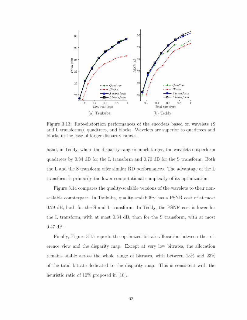
(a) Tsukuba

��� ��� ��� ��� �

��

��

�

��

�

��

������ ����� �

�� � ���

��������

������

������������

�� ����������

(b) Teddy

Figure 3.13: Rate-distortion performances of the encoders based on wavelets (Sand L transforms), quadtrees, and blocks. Wavelets are superior to quadtrees andblocks in the case of larger disparity ranges.

hand, in Teddy, where the disparity range is much larger, the wavelets outperform

quadtrees by 0.84 dB for the L transform and 0.70 dB for the S transform. Both

the L and the S transform offer similar RD performances. The advantage of the L

transform is primarily the lower computational complexity of its optimization.

Figure 3.14 compares the quality-scalable versions of the wavelets to their non-

scalable counterpart. In Tsukuba, quality scalability has a PSNR cost of at most

0.29 dB, both for the S and L transform. In Teddy, the PSNR cost is lower for

the L transform, with at most 0.34 dB, than for the S transform, with at most

0.47 dB.

Finally, Figure 3.15 reports the optimized bitrate allocation between the ref-

erence view and the disparity map. Except at very low bitrates, the allocation

remains stable across the whole range of bitrates, with between 13% and 23%

of the total bitrate dedicated to the disparity map. This is consistent with the

heuristic ratio of 10% proposed in [10].

62

������������ �����������

������������������

������������ ���� �������

������������ ��������

��� ��� ��� ���

����� ���� ����

��

��

�

��

��

��

�������

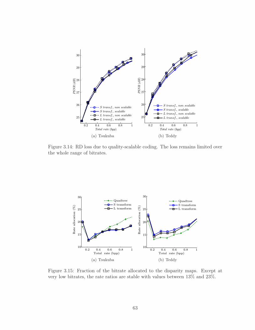
(a) Tsukuba

������������ �����������

������������������

������������ ���� �������

������������ ��������

��� ��� ��� ���

����� ���� ����

��

��

�

��

��

��

�������

(b) Teddy

Figure 3.14: RD loss due to quality-scalable coding. The loss remains limited overthe whole range of bitrates.

��

��

��

��

��

������� ��������

������

����������

����������

��� ��� ��� ��� � ��������!""�

(a) Tsukuba

��

��

��

��

��

��

������� ��������

������

����������

����������

��� ��� ��� ��� � ��������!""�

(b) Teddy

Figure 3.15: Fraction of the bitrate allocated to the disparity maps. Except atvery low bitrates, the rate ratios are stable with values between 13% and 23%.

63

3.5 Conclusion

This chapter has proposed a novel wavelet-domain DIBR codec able to approxi-

mate static plenoptic functions inside a ROI. The wavelet coefficients for both the

images and the disparity maps have been estimated and encoded jointly to provide

an optimized bitrate allocation and reduce the ambiguity of the disparity estima-

tion. In spite of the nonlinearity of the optimization problem, a globally optimal

encoding of the disparity maps has been found using dynamic programming along

the tree of integer wavelet coefficients. In addition to the resolution scalability

intrinsic to wavelets, quality scalability has been introduced using quality layers.

Finally, experimental results on real data have confirmed the performances of the

proposed codec. Future work will aim to extend the optimization of the disparity

map to more general integer wavelets, mitigate the issues due to occlusions, and

compress dynamic plenoptic functions.

64

CHAPTER 4

JOINT ENCODING OF THEDIBR USINGSHAPE-ADAPTIVE WAVELETS

4.1 Introduction

Free-viewpoint three-dimensional television (3D-TV) provides an enhanced view-

ing experience in which users are able to perceive the third spatial dimension and

are free to move inside the 3D video [47]. With the advent of multiview autostereo-

scopic displays [47], 3D-TV is expected to be the next evolution of television after

high definition.

Three-dimensional television poses new technological challenges, which include

recording, encoding, and displaying 3D videos. At the core of these challenges

lies the massive amount of data required to represent the set of all possible views,

called the plenoptic function [24], or at least a realistic approximation of them.

The depth image based representation (DIBR) has recently

emerged as an effective approach [10], which allows both compact data repre-

sentation and realistic view synthesis. As shown in Figure 4.1, the DIBR is made

of pairs of images and depth maps, each of which provides a local approximation

of the plenoptic function. At the decoder, arbitrary views are synthesized from the

DIBR using image-based rendering [24].

Each pair of image and depth map can be seen as a four-channel image with

one channel for luma, two for chroma and one for depth. Therefore, classical im-

age and video codecs like MPEG-2, H.264/AVC, and JPEG2000 only need minor

modifications to be able to handle DIBRs [10, 47]. This approach however fails to

65

(a) Depth map and edges (b) Image and edges

Figure 4.1: Input data of the proposed DIBR codec: shared edges superimposedover a depth map (a) and an image (b).

take into consideration the fact that images and depth maps exhibit widely differ-

ent statistics, which make classical transforms like the discrete wavelet transform

(DWT) or the discrete cosine transform (DCT) ill-suited to encode DIBRs. In

particular, depth maps tend to contain sharper edges than images, which create

streaks of large coefficients in the transform domain.

In [74], it was shown that a representation based on platelets, which assumes

piecewise planar areas separated by piecewise linear edges, could lead to major

rate-distortion (RD) gains. However, the practical use of platelets is limited by

the computational cost of encoding. Unlike standard image codecs which rely on

fast transforms (such as DCT or DWT), quantizers, and entropy coders to encode

the data [19], platelets require the encoder to solve a complex RD optimization

problem.

Moreover, both platelet-based codecs and standard image codecs ignore another

source of data redundancy: the correlation between depth edges and image edges.

Indeed, the 3D scenes are usually made of objects with well-defined surfaces, which,

by projection onto the camera image plane, create edges at the same locations in

the depth map and the image.

66

In this chapter, we propose a codec which takes into account both sources of re-

dundancies. It encodes the locations of the major depth edges explicitly and treats

the regions they separate as independent during the wavelet transform by using an

extension of the shape-adaptive discrete wavelet transform (SA-DWT) [75]. The

proposed SA-DWT generates small wavelet coefficients both in smooth regions and

along the encoded edges. It is efficiently computed using lifting [19], a procedure

which is fast, in place, simple to implement, and trivially invertible. Moreover, the

explicit edge coding allows the codec to share the edge information between the

depth map and the image, which reduces their joint redundancy.

Thus the proposed codec amounts to a simple modification of a scheme that

independently codes depth and image using wavelet-based codecs. As a result, we

can benefit from the large body of existing work on wavelet-based codecs. However,

as we shall see, this modification leads to significant gains, up to 5.46 dB.

The remainder of the chapter is organized as follows. An overview of the

proposed codec is presented in Section 4.2. A detailed description of its components

is given in Sections 4.3, 4.4, and 4.5, which consider respectively the SA-DWT, the

handling of edges during lifting, and edge coding. Finally, Section 4.6 presents

experimental results.

4.2 Proposed Codec

As shown in Figure 4.2, the proposed DIBR encoder takes three signals as input,

which represent respectively the depth map, the image, and the edges. The DIBR

encoder is made of two wavelet encoders [19], one processing the depth map and

the other the image. Like standard wavelet encoders, each is made of a wavelet

transform followed by quantization and entropy coding. The DIBR decoder simply

inverses each of these steps in reverse order.

67

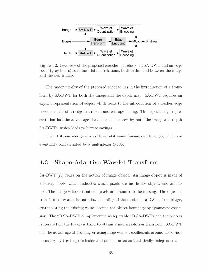
Figure 4.2: Overview of the proposed encoder. It relies on a SA-DWT and an edgecoder (gray boxes) to reduce data correlations, both within and between the imageand the depth map.

The major novelty of the proposed encoder lies in the introduction of a trans-

form by SA-DWT for both the image and the depth map. SA-DWT requires an

explicit representation of edges, which leads to the introduction of a lossless edge

encoder made of an edge transform and entropy coding. The explicit edge repre-

sentation has the advantage that it can be shared by both the image and depth

SA-DWTs, which leads to bitrate savings.

The DIBR encoder generates three bitstreams (image, depth, edge), which are

eventually concatenated by a multiplexer (MUX).

4.3 Shape-Adaptive Wavelet Transform

SA-DWT [75] relies on the notion of image object. An image object is made of

a binary mask, which indicates which pixels are inside the object, and an im-

age. The image values at outside pixels are assumed to be missing. The object is

transformed by an adequate downsampling of the mask and a DWT of the image,

extrapolating the missing values around the object boundary by symmetric exten-

sion. The 2D SA-DWT is implemented as separable 1D SA-DWTs and the process

is iterated on the low-pass band to obtain a multiresolution transform. SA-DWT

has the advantage of avoiding creating large wavelet coefficients around the object

boundary by treating the inside and outside areas as statistically independent.

68

This is this idea of statistically independent areas that we shall use to efficiently

code the DIBR. In our case, however, there is no single object. Instead, the DIBR

is made of multiple superimposed objects. This issue is overcome by replacing the

binary mask by a binary edge map and by treating the areas on opposite sides of

the edges as statistically independent.

Figure 4.3 presents an example of signal processed by the proposed SA-DWT.

The SA-DWT clearly creates much less nonzero wavelet coefficients around edges

than the standard DWT, which leads to bitrate savings. SA-DWT has the dis-

advantage of requiring a bitrate overhead to code the edge location. However,

experiments show that this overhead is more than compensated by the savings.

We rely on lifting [19] to implement the 1D SA-DWT. First, we present the

standard lifting and then describe the modifications making it shape adaptive. The

lifting splits the samples at odd and even locations into two cosets and modifies

them alternatively using a series of “steps.”

By convention, lifting begins by modifying the odd coset by a so-called “predict”

step, which transforms a signal x into a signal y such that

y2t = x2t,

y2t+1 = x2t+1 + λ2k(x2t + x2t+2),

(4.1)

where t denotes the sample locations, 2k the step number, and λ2k a weight. The

even coset is modified by a so-called “update” step, which transforms a signal x

into a signal y such that

y2t = x2t + λ2k+1(x2t−1 + x2t+1),

y2t+1 = x2t+1.

(4.2)

Figure 4.4 shows a graphical example of these lifting steps. Weights λ for

69

(a) Signal made of constant, linear and cubic pieces. The dashed red lines indicateedges.

(b) High-pass bands of a standard 9/7DWT with symmetric extension.

(c) High-pass bands of a 9/7 SA-DWTwith cubic extension.

Figure 4.3: Comparison of standard and shape adaptive DWTs. In the latter case,all but the coarsest high-pass band are zero.

70

Figure 4.4: The four lifting steps associated with a 9/7 wavelet, which transformthe signal x first into a and then into y. The values x2t+2 and a2t+2 on the otherside of the edge (dashed vertical line) are extrapolated. They have dependencieswith the values inside the two dashed triangles.

classical wavelets like the 5/3 or the 9/7 can be found in [19]. After the final

update step, the odd coset contains the high-pass coefficients and the even coset

the low-pass ones.

Standard lifting is made shape adaptive by modifying (4.1) and (4.2) at lo-

cations where they would perform a weighted addition of two samples xt and xt′

separated by an edge. In that case, the sample xt′ which is not on the same side of

the edge as the sample yt being computed is considered missing and is extrapolated

from samples on the same side as yt. Designing effective extrapolation methods is

the topic of the following section.

71

4.4 Lifting Edge Handling

Our goal is to design extrapolation methods which lead to null high-pass coefficients

around edges. The symmetric extension [75] ensures the continuity of the signal

across the edge but not of its higher order derivatives. Therefore, even wavelets

which zero out high-order polynomials are not able to zero them out near edges.

The extrapolation design we now present is able to overcome this limitation.

In the following, we only consider extrapolation on the right side of edges, as

shown in Figure 4.4. Left-side extrapolation follows by symmetry. Let us assume

that there is an edge at T + 1/2 and that left of this edge the signal is polynomial

of degree L, that is,

xt =

L∑

k=0

αktk, ∀t ≤ T. (4.3)

In order for lifting to be performed, some of the samples on the right side of

the edge need to be estimated. In Figure 4.4, where T = 2t + 1, these samples

are x2t+2 and a2t+2. We choose to extrapolate them using a weighted sum of the

samples on the left of the edge, using an equation of the form

zT+1 =

L∑

k=0

µkzT−1−2k (4.4)

where z denotes the signal and µ the vector of unknown weights. The extrapolation

only relies on samples from the same coset to maintain invertibility and in-place

computation.

If the wavelet zeroes out polynomials of degree L, all high-pass coefficients left

of the edge should be zero. Among all these equations, only those near the edge

depend on µ. In Figure 4.4, this corresponds to y2t−1 and y2t+1. We write them

as functions of µ, λ, and T using (4.1), (4.2), (4.3), and (4.4). Setting them to

zero gives a system of polynomials in T . We want the solution to be invariant

72

to even shifts of the edge, which means that the polynomials must be identically

zero. Therefore all the polynomial coefficients are zero, which gives rise to L new

equations per polynomial. The unknown weights µ are obtained by solving this

system of equations.

Writing and solving the equations may be quite tedious but can be easily done

by mathematical software and the solutions are particularly simple. In the case

of 5/3 wavelets, which zeroes out linear polynomials, an extrapolation with L = 0

gives the standard symmetric extension with µ = 1 and an extrapolation with L =

1 gives a linear extension with µ = [ 2 −1 ]. In the case of the 9/7, which zeroes

out cubic polynomials, both of these extrapolations hold true and an extrapolation

with L = 3 gives a cubic extension with µ = [ 4 −6 4 −1 ]. The effectiveness

of this latter extrapolation is demonstrated in Figure 4.3.

The proposed method fails in two cases. First, when the edge location is of

the form 2t + 1/2, the unknown high-pass coefficient y2t+1 has a dependency with

the low-pass coefficient y2t but not with any high-pass coefficient on the left of the

edge. There is therefore no equation available to solve its extrapolation. However,

we can assume that the polynomial is perfectly fitted on the right side of the

edge, which means that y2t+1 is zero. The extrapolation also fails when there is an

insufficient number of samples between two edges. In that case, the order L of the

extrapolation is reduced.

4.5 Edge Representation and Coding

The SA-DWT requires an explicit knowledge of the edge locations. In 1D, these

edges are located at half-integer locations between samples. In 2D, they are lo-

cated between samples along rows and columns, which gives rise to an edge lattice

dual to the sample lattice, as shown in Figure 4.5. Edges are either horizontal,

73

Figure 4.5: Example of the dual lattices of samples and edges. Each edge indicatesthe statistical independence of the two half rows or half columns of samples itseparates.

splitting columns, or vertical, splitting rows. We represent them by two binary

edge maps, denoted respectively e(h)s+1/2,t and e

(v)s,t+1/2 where s and t denote integer

spatial locations.

Moreover, the SA-DWT is a multiresolution transform where each low-pass

band must be associated with a pair of edge maps. Let use denote by xs,t,j the

samples at resolution level j and by e(h)s+1/2,t,j and e

(v)s,t+1/2,j the associated depth

maps. The pyramid of edge maps is obtained by iterative downsampling using the

equations

e(h)s+1/2,t,j = max

(

e(h)2s+1/2,2t,j−1, e

(h)2s+1+1/2,2t,j−1

)

e(v)s,t+1/2,j = max

(

e(v)2s,2t+1/2,j−1, e

(v)2s,2t+1+1/2,j−1

)

. (4.5)

The edge maps at the finest resolution j = 0 are encoded using a differential

Freeman chain code inspired from [76]. Each edge along the chain can take one of

the four directions {right, up, left, down} numbered from 0 to 3. The direction of

the nth edge is denoted dn and the differential direction ∆n between two consecutive

edges is defined by

∆n = dn − dn−1. (4.6)

74

Directions are recovered iteratively from differential directions using the equation

dn = dn−1 + ∆dn mod 4 (4.7)

where mod denotes the modulo operator.

The chain code is made of a chain header which stores the location of the

first edge end-point and the first direction and a chain body which stores the

differential directions. In the example of Figure 4.5, the chain code is 14+½, 23+½;0 ; -1, 0, 0, +1, 0. Finally, the chain code is entropy coded to generate the

bitstream. Fixed-length codes are used for the header and simple variable-length

codes {−1 : 10, 0 : 0, +1 : 11} are used for the body, to take advantage of the

large number of zeros.

4.6 Experimental Results

We present experimental results on the Teddy set, shown in Figure 4.1. The DIBR

is 375×450 in size with intensities in the range [0, 255] and depths in [0, 53]. For

simplicity, only the luma channel of the image is considered. Missing values in the

depth maps have been interpolated using in-painting. Edges have been obtained

in a semiautomatic way by applying a Canny edge detector to the depth map and

letting the user choose which edge chains to keep.

We compare the performances of two codecs: one based on the DWT and the

other on the proposed SA-DWT with explicit edge coding. Both codecs perform

a five-level decomposition and rely on the same quantizer and entropy coder, pro-

vided by the SPIHT implementation of the QccPack library. They also rely on the

same 9/7 wavelet for the transform, which is the main wavelet in JPEG2000 [19].

Following [77], both codecs allocate 20% of the bitrate to the depth.

75

(a) Std9/7sym (b) SA9/7lin

Figure 4.6: Absolute values of the high-pass coefficients of the depth map usingstandard and shape-adaptive wavelets. The latter provides a much sparser decom-position.

The two codecs differ in their handling of edges: the DWT-based codec uses the

standard 9/7 wavelet with symmetric extension, denoted “std9/7sym,” while the

SA-DWT-based codec uses the shape-adaptive 9/7 wavelet with linear extension,

denoted “SA9/7lin,” for the depth map and the shape-adaptive 9/7 wavelet with

symmetric extension, denoted “SA9/7sym,” for the image. The SA-DWT-based

codec also includes an edge codec, as shown in Figure 4.2. The experiments are

based on the edge map shown in Figure 4.1, which has a bitrate overhead of

0.015 bpp.

Figure 4.6 shows the wavelet coefficients of the depth map obtained using

std9/7sym and SA9/7lin. The standard transform exhibits large values along

edges, which are absent from the shape-adaptive transform. The entropy of the

latter is therefore much reduced.

Figure 4.7 shows the reconstructed depth map at 0.04 bpp using the standard

and shape-adaptive codecs. Even at low bitrates, the latter reconstructs sharp

edges and avoids Gibbs artifacts along edges. Moreover, the sparser nature of the

SA-DWT coefficients means that the shape-adaptive codec is able to spend more

76

(a) Std9/7sym - 36.21 dB (b) SA9/7lin - 39.86 dB

Figure 4.7: Reconstruction of the depth map at 0.04 bpp using standard andshape-adaptive wavelets. The latter gives sharp edges free of Gibbs artifacts.

bits outside edge areas, which leads for instance to a slightly better reconstruction

of the bottom right of the depth map.

Figure 4.8(a) compares the RD performances of the two codecs for the depth

map. The bitrate consists in the wavelet coefficients, along with the edges in

the shape-adaptive case. The figure shows that the edge overhead is more than

compensated by the reduced entropy of the wavelet coefficients. This leads to

PSNR gains over the whole bitrate range, achieving up to 5.46 dB.

Figure 4.8(b) compares the RD performances of the two codecs for the image.

The bitrate is made of the wavelet coefficients in both cases, the edge overhead

having been accounted for in the depth bitrate. The figure shows PSNR gains over

the whole bitrate range, achieving up to 0.19 dB.

4.7 Conclusion

We have presented a novel codec of DIBRs for free-viewpoint 3D-TV. By replacing

the DWT of classical image codecs by a SA-DWT and adding an edge encoder, we

have been able to obtain significant PSNR gains, achieving up to 5.46 dB. Future

work shall consider the automatic extraction of edges based on RD considerations.

77

(a) Depth map (b) Image

Figure 4.8: Rate-distortion performances of standard and shape-adaptive wavelets.The latter gives PSNR gains of up to 5.46 dB on the depth map and 0.19 dB onthe image.

78

CHAPTER 5

3D MODEL-BASED FRAMEINTERPOLATION FOR DVC

5.1 Introduction

Distributed source coding (DSC) has gained interest for a range of applications such

as sensor networks, video compression, or loss-resilient video transmission. DSC

finds its foundation in the seminal Slepian-Wolf [78] and Wyner-Ziv [79] theorems.

Most Slepian-Wolf and Wyner-Ziv coding systems are based on channel coding

principles [80–86]. The statistical dependence between two correlated sources X

and Y is modeled as a virtual correlation channel analogous to binary symmet-

ric channels or additive white Gaussian noise (AWGN) channels. The source Y

(called the side information) is thus regarded as a noisy version of X (called the

main signal). Using error correcting codes, the compression of X is achieved by

transmitting only parity bits. The decoder concatenates the parity bits with the

side information Y and performs error correction decoding, i.e., MAP or MMSE

estimation of X given the received parity bits and the side information Y .

Compression of video streams can be cast into an instance of side information

coding, as shown by Aaron et al. [87–89] and Puri et al. [90–92]. These schemes

are also referred to as distributed video coding (DVC) systems. A comprehensive

survey of distributed video compression can be found in [93]. One key aspect in the

performance of the system is the mutual information between the side information

and the information being Wyner-Ziv encoded. In current approaches, the side

information is generated via motion-compensated frame interpolation, often using

79

block-based motion compensation (BBMC) [93]. Motion fields are first computed

between key frames, which may be distant from one another. An interpolated

version of these motion fields is then used to generate the side information for

each WZ frame. The frame interpolation based on these interpolated motion fields

is not likely to lead to the highest possible PSNR, hence to the highest mutual

information between the side information and the Wyner-Ziv encoded frame. To

cope with these limitations, BBMC is embedded in a multiple motion hypothesis

framework in [93,94]. The actual motion vectors are chosen by testing the decoded

frames against hash codes or CRCs.

Here, we address the problem of side information generation in distributed cod-

ing of videos captured by a camera moving in a 3D static environment with Lam-

bertian surfaces. This problem is of particular interest to specialized applications

such as augmented reality, remote controlled robots operating in hazardous envi-

ronments, and remote exploration by drones or planetary probes. We explore the

benefits of more complex motion models belonging to the Structure-from-Motion

(SfM) paradigm [16]. These motion models exhibit strong geometrical properties,

which allow their parameters to be robustly estimated. Note that, unlike predic-

tive coding, DVC has the advantage of not requiring the transmission of motion

model parameters. Therefore, increasing the complexity of motion models, and

thus their ability to accurately represent complex motions, offers potential gains

in mutual information without additional bitrate overheads.

When used in computer vision applications, SfM approaches aim at generating

visually pleasing virtual views [8]. On the other hand, when used in DVC, the

objective is to generate intermediate frames (the side information) with the highest

PSNR. This requires a reliable estimation of the camera parameters as well as

sub-pel precision of the reprojected 3D model, especially in edge regions where

even small misalignments can have a strong impact on the PSNR. In addition,

80

constraints on latency in applications such as video streaming, as well as memory

constraints, prevent the reconstruction of the 3D scene from all the key frames at

once, as is usually done in SfM. Instead, a sequence of independent 3D models is

reconstructed from pairs of consecutive key frames.

In this chapter, we first describe two 3D model-based frame interpolation meth-

ods relying on SfM techniques, one block-based and one mesh-based, both being

constrained by the epipolar geometry. These first approaches suffer from the follow-

ing limitation. The motion fields associated with the intermediate frames are inter-

polated with the classical assumption of linear motion between key frames. This

creates misalignments between the side information and the actual WZ frames,

which have a strong impact on the rate-distortion (RD) performances of the 3D

model-based DVC solution.

This observation led us to introduce two methods to estimate the intermediate

motion fields with the help of point tracks, instead of interpolating them. The

motion fields are thus obtained by computing the camera parameters at interme-

diate time instants using point tracks. A first technique relies on feature point

tracking at the decoder, each frame being processed independently at the encoder.

In addition to the key frames, the encoder extracts and transmits a limited set

of feature points which are then linked temporally at the decoder. Feature point

tracking at the decoder greatly reduces misalignments, thereby increasing the side

information PSNR with, in turn, a significant impact on the RD performances of

the 3D model-based DVC system. These performances are then further improved

by introducing the tracking at the encoder. The encoder thus shares some limited

information between frames under the form of intensity patches to construct the

tracks sent to the decoder. The latter method has the additional advantage of giv-

ing the encoder a rough estimation of the video motion content, which is sufficient

to decide when to send key frames. Note that the problem of key frame selection

81

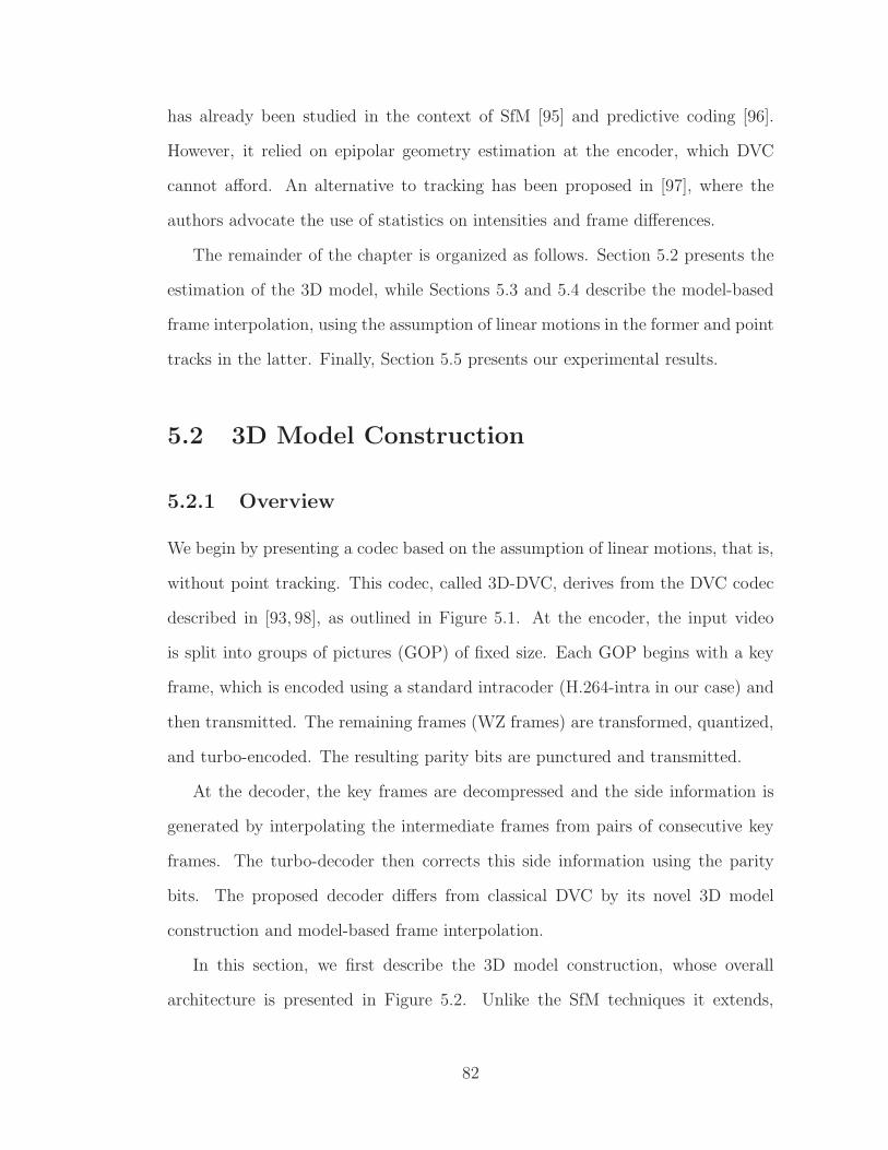
has already been studied in the context of SfM [95] and predictive coding [96].

However, it relied on epipolar geometry estimation at the encoder, which DVC

cannot afford. An alternative to tracking has been proposed in [97], where the

authors advocate the use of statistics on intensities and frame differences.

The remainder of the chapter is organized as follows. Section 5.2 presents the

estimation of the 3D model, while Sections 5.3 and 5.4 describe the model-based

frame interpolation, using the assumption of linear motions in the former and point

tracks in the latter. Finally, Section 5.5 presents our experimental results.

5.2 3D Model Construction

5.2.1 Overview

We begin by presenting a codec based on the assumption of linear motions, that is,

without point tracking. This codec, called 3D-DVC, derives from the DVC codec

described in [93, 98], as outlined in Figure 5.1. At the encoder, the input video

is split into groups of pictures (GOP) of fixed size. Each GOP begins with a key

frame, which is encoded using a standard intracoder (H.264-intra in our case) and

then transmitted. The remaining frames (WZ frames) are transformed, quantized,

and turbo-encoded. The resulting parity bits are punctured and transmitted.

At the decoder, the key frames are decompressed and the side information is

generated by interpolating the intermediate frames from pairs of consecutive key

frames. The turbo-decoder then corrects this side information using the parity

bits. The proposed decoder differs from classical DVC by its novel 3D model

construction and model-based frame interpolation.

In this section, we first describe the 3D model construction, whose overall

architecture is presented in Figure 5.2. Unlike the SfM techniques it extends,

82

Figure 5.1: Outline of the codec without point tracking (3D-DVC). The proposedcodec benefits from an improved motion estimation and frame interpolation (grayboxes).

Figure 5.2: Outline of the 3D model construction.

the proposed model construction focuses on the PSNR of the interpolated frames

to maximize the quality of the side information. Toward that goal, we present

a novel robust correspondence estimation with subpixel accuracy. In particular,

correspondences are scattered over the whole frames and are dense in areas of high

gradients. Furthermore, the 3D model construction is robust to quantization noise.

After introducing some notation, we shall first describe the camera parameter

estimation and then the correspondence estimation.

5.2.2 Notation

We shall use the typesettings a, a,A to denote respectively scalars, column vectors,

and matrices. In the following, a(t)j (i) denotes the jth scalar-entry of the ith vector

of a set at time t. Likewise for matrices, Aij denotes the scalar entry at the ith row

and jth column, while Ai: represents its ith row vector. Moreover, A⊺ denotes the

83

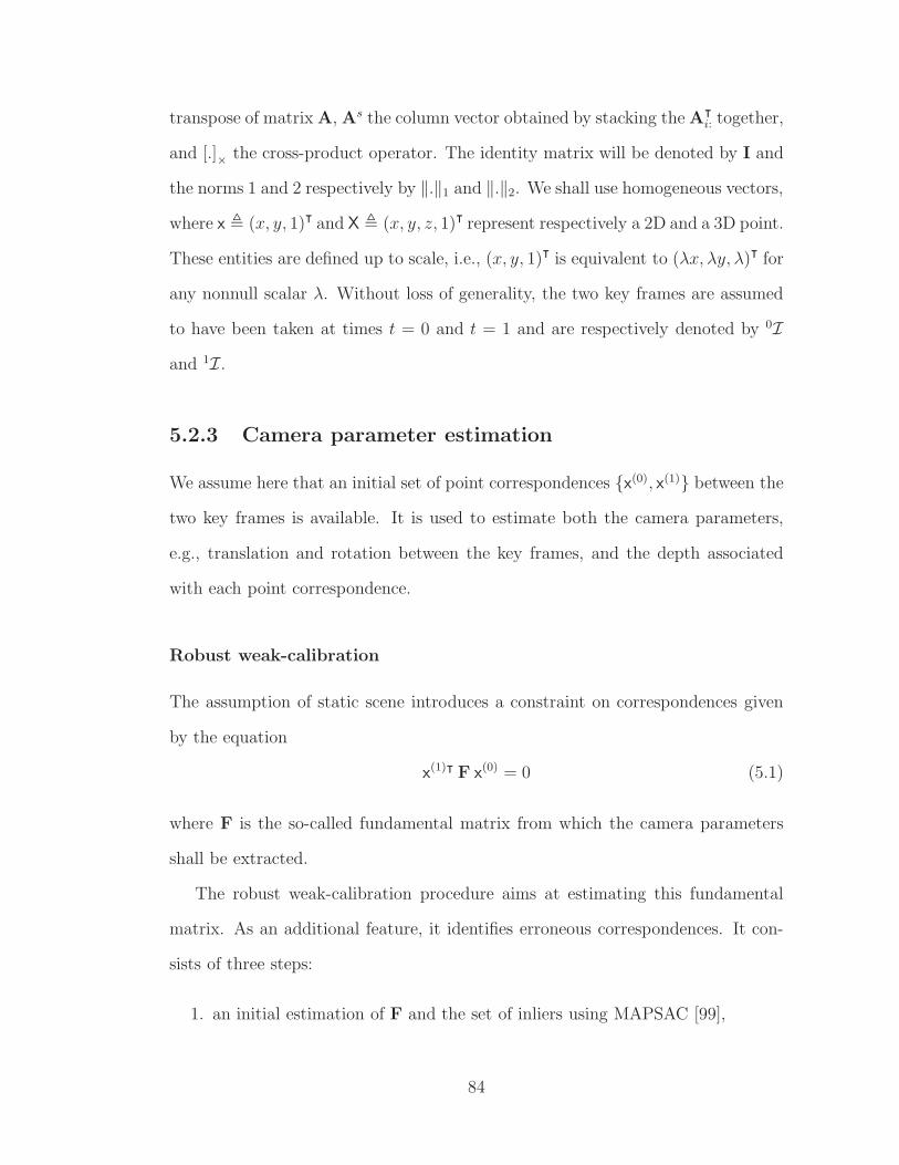
transpose of matrix A, As the column vector obtained by stacking the A⊺

i: together,

and [.]× the cross-product operator. The identity matrix will be denoted by I and

the norms 1 and 2 respectively by ‖.‖1 and ‖.‖2. We shall use homogeneous vectors,

where x , (x, y, 1)⊺ and X , (x, y, z, 1)⊺ represent respectively a 2D and a 3D point.

These entities are defined up to scale, i.e., (x, y, 1)⊺ is equivalent to (λx, λy, λ)⊺ for

any nonnull scalar λ. Without loss of generality, the two key frames are assumed

to have been taken at times t = 0 and t = 1 and are respectively denoted by 0I

and 1I.

5.2.3 Camera parameter estimation

We assume here that an initial set of point correspondences {x(0), x(1)} between the

two key frames is available. It is used to estimate both the camera parameters,

e.g., translation and rotation between the key frames, and the depth associated

with each point correspondence.

Robust weak-calibration

The assumption of static scene introduces a constraint on correspondences given

by the equation

x(1)⊺ F x(0) = 0 (5.1)

where F is the so-called fundamental matrix from which the camera parameters

shall be extracted.

The robust weak-calibration procedure aims at estimating this fundamental

matrix. As an additional feature, it identifies erroneous correspondences. It con-

sists of three steps:

1. an initial estimation of F and the set of inliers using MAPSAC [99],

84

2. a first refinement of F and the set of inliers using LO-RANSAC [100],

3. a second refinement of F over the final set of inliers by a nonlinear minimiza-

tion of the Sampson distance [16].

Quasi-Euclidean self-calibration and triangulation

The next step is to recover the projection matrices P and the depths λ. We can

choose the world coordinate system (WCS) of the 3D scene to be the camera

coordinate system at time t = 0, leading to P(0) = [I 0]. This leaves four degrees

of freedom in the WCS. They appear in the relation between F and the projection

matrix of the second key frame P(1) , [R(1) t(1)], given by

t(1) ∈ ker (F⊺) and R(1) = [t(1)]×F− t(1) a⊺ (5.2)

where a is an arbitrary 3-vector and t(1) has arbitrary norm. For the time being,

these degrees of freedom are fixed by choosing t(1) with unit norm and setting

a = t(0), where the epipoles t(0) and t(1) are recovered from the singular value

decomposition (SVD) of the matrices F and F⊺, respectively [16]. Since projec-

tion matrices are defined up-to-scale, in the remainder of the chapter they are

normalized so that their Frobenius norm will be√

3.

The depths can then be recovered. Let a 3D point X project itself onto a 2D

point x on the camera image plane. These two points are related by λx = PX

where λ is the projective depth. Therefore, correspondences allow the recovery of

a cloud of 3D points by triangulation, solving the system of equations

λ(1)x(1) = λ(0)R(1)x(0) + t(1) (5.3)

for each correspondence.

85

The initial choice of WCS is refined by quasi-Euclidean self-calibration [101],

so that the WCS is as Euclidean as possible. We also constrain the depths in

the new WCS to be bounded by 1 and M to reduce numerical issues during the

bundle adjustment detailed later. Assuming that the camera parameters cannot

undergo large variations between key frames, we look for a matrix R(1) as close

as possible to the identity matrix and compatible with the fundamental matrix F.

The optimal vector a is then found by minimizing∥

∥R(1) − t(1) at − I∥

∥

1under the

linear constraints

max(λ(0), λ(1))/M ≤ λ(0)x(0)⊺a− 1 ≤ min(λ(0), λ(1)). (5.4)

A lower bound on the value of M is given by max(λ(0), λ(1))/ min(λ(0), λ(1)). The

self-calibration starts with this value and increases it until the linear programming

problem admits a solution.

Bundle adjustment

The camera parameters and the depths obtained so far suffer from the bias inherent

to linear estimation [102]. They can be refined by minimizing their Euclidean

reprojection error on the key frames. First, the basis of the projective space has

to be fixed to prevent it from drifting. This is done by fixing two 3D points

and performing the optimization over a reduced parameter space. As shown in

Appendix A, the 12-dimensional projection matrix P(1) can be expressed as a

linear combination of an 8-dimensional unit vector r, i.e., P(1)s =√

3Wr where W

is an orthonormal matrix. The two fixed 3D points are chosen randomly under the

constraints that they have small reprojection errors and that they are far from the

epipoles and from each other.

86

The minimization of the Euclidean reprojection error is defined as

min{λ(0)},r

J(

{x(0)}, {λ(0)}, {x(1)},√

3Wr)

such that ‖r‖2 = 1

(5.5)

where J is the euclidean reprojection error given by

J(

{x(0)}, {λ(0)}, {x(t)},P(t)s)

,

∑

i

(

x(t)(i)−[

λ(0)(i)x(0)⊺(i) 1]

P(t)s1:4

[λ(0)(i)x(0)⊺(i) 1]P(t)s9:12

)2

+∑

i

(

y(t)(i)−[

λ(0)(i)x(0)⊺(i) 1]

P(t)s5:8

[λ(0)(i)x(0)⊺(i) 1]P(t)s9:12

)2

.

(5.6)

The minimization is solved using an alternated reweighted linear least square ap-

proach [103], as detailed in Appendix B. A refined fundamental matrix is then

deduced using F = [t(1)]×R(1) and refined point correspondences are obtained us-

ing reprojection.

5.2.4 Correspondence estimation

We now turn to the estimation of the set of point correspondences {x(0), x(1)}

between the two key frames.

Feature point detection

First, feature points {x} are detected on each key frame independently. We use

the Harris-Stephen corner detector [104] to find feature points. Its sensitivity is

adapted locally to spread feature points over the whole frame [16], which improves

the weak-calibration detailed previously.

87

Feature point matching

Feature points are then matched across key frames to form correspondences. All

pairs of feature points{

x(0), x(1)}

are considered as candidate correspondences. A

first series of tests eliminates blatantly erroneous correspondences:

1. Correspondences with very large motions are discarded.

2. Correspondences with dissimilar intensity distributions in the neighborhoods

around feature points are discarded. Distributions are approximated using

Parzen windows [105, §4.3] and sampled uniformly to obtain histograms. The

similarity of histograms is tested using the χ2-test [66, §14.3].

Subpixel refinement

The locations of the remaining correspondences are then refined locally by search-

ing for the least mean square error (MSE) between neighborhoods around feature

points. The minimization is solved using the Levenberg-Marquardt algorithm [66,§15.5]. This refinement compensates for errors from the Harris-Stephen detector,

leads to values of MSE independent of image sampling [106], and computes feature

point locations with subpixel accuracy.

Outlier removal

A second series of tests is applied to eliminate erroneous correspondences. These

tests are performed when camera parameter estimation provides the necessary

information (see Figure 5.2).

1. MSE: Correspondences with large MSE are discarded.

2. Unicity: Each feature point is only allowed to belong to at most one cor-

respondence. This unicity constraint is enforced using the Hungarian algo-

88

rithm [68, §I.5], which keeps only the correspondences with the least MSE

when the unicity constraint is violated.

3. Epipolar: Correspondences identified as outliers during the robust weak-ca-

libration are discarded.

4. Motion: Correspondences with aberrant motion are removed by testing the

difference between their motion and the weighted median of the motions of

their neighbors positioned on Delaunay triangles [107, Chap. 9]. Neighbors

are assigned weights inversely proportional to their distances.

5. Reprojection: The projection of the 3D points must be close to the actual

2D points.

6. Chirality: All products of projective depths λ(0)λ(1) must have the same

sign [108, Th. 17],

7. Epipole: Correspondences must be far from epipoles, since triangulation is

ill-conditioned around them.

8. Depth: Points with aberrant depths compared to the depths of their neigh-

bors are removed.

Correspondence propagation

The set of correspondences obtained so far is reliable and accurate but still fairly

sparse. It is first densified over unmatched feature points by increasing the toler-

ance of the tests described previously and enforcing motion smoothness using the

weighted median of neighboring motions.

Correspondences are then propagated along edges, under the epipolar con-

straint. The goal of this procedure is to get accurate motion information in edge

89

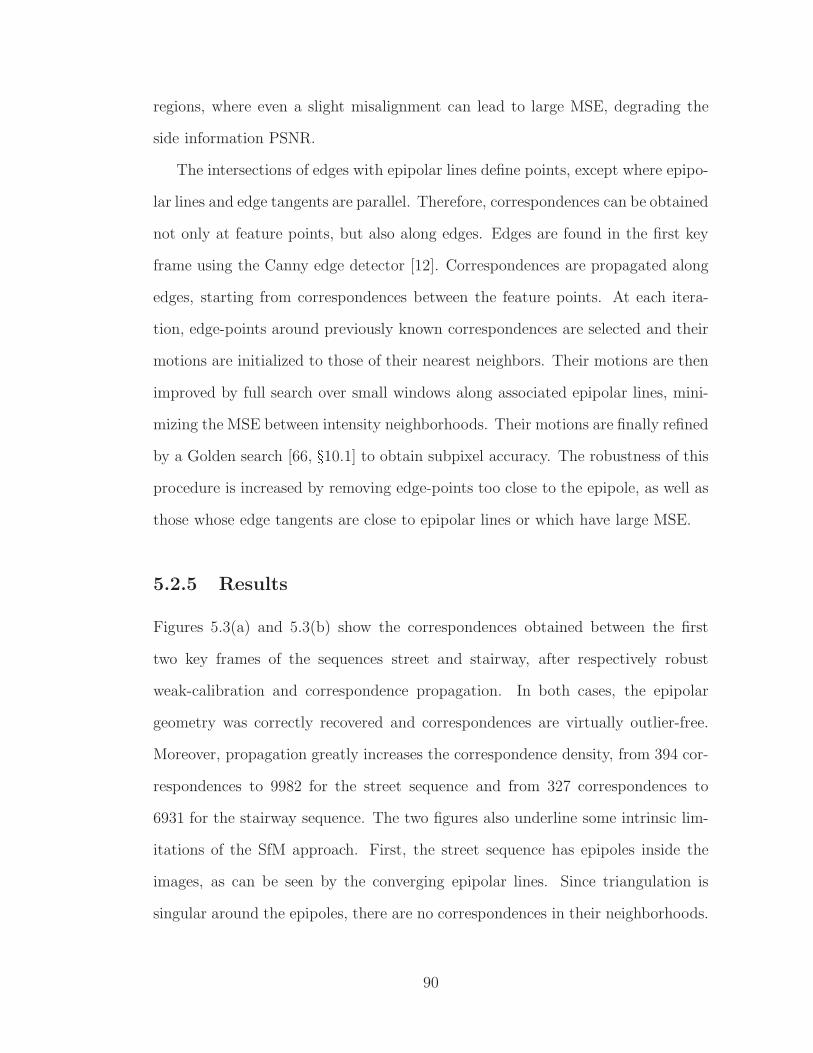
regions, where even a slight misalignment can lead to large MSE, degrading the

side information PSNR.

The intersections of edges with epipolar lines define points, except where epipo-

lar lines and edge tangents are parallel. Therefore, correspondences can be obtained

not only at feature points, but also along edges. Edges are found in the first key

frame using the Canny edge detector [12]. Correspondences are propagated along

edges, starting from correspondences between the feature points. At each itera-

tion, edge-points around previously known correspondences are selected and their

motions are initialized to those of their nearest neighbors. Their motions are then

improved by full search over small windows along associated epipolar lines, mini-

mizing the MSE between intensity neighborhoods. Their motions are finally refined

by a Golden search [66, §10.1] to obtain subpixel accuracy. The robustness of this

procedure is increased by removing edge-points too close to the epipole, as well as

those whose edge tangents are close to epipolar lines or which have large MSE.

5.2.5 Results

Figures 5.3(a) and 5.3(b) show the correspondences obtained between the first

two key frames of the sequences street and stairway, after respectively robust

weak-calibration and correspondence propagation. In both cases, the epipolar

geometry was correctly recovered and correspondences are virtually outlier-free.

Moreover, propagation greatly increases the correspondence density, from 394 cor-

respondences to 9982 for the street sequence and from 327 correspondences to

6931 for the stairway sequence. The two figures also underline some intrinsic lim-

itations of the SfM approach. First, the street sequence has epipoles inside the

images, as can be seen by the converging epipolar lines. Since triangulation is

singular around the epipoles, there are no correspondences in their neighborhoods.

90

(a) Epipolar geometry after robust weak calibration

(b) Correspondences after propagation along edges

Figure 5.3: Correspondences and epipolar geometry between the two first losslesskey frames of the sequences street and stairway. Feature points are represented byred dots, motion vectors by magenta lines ending at feature points, and epipolarlines by green lines centered at the feature points.

Second, the stairway sequence contains strong horizontal edges whose tangents are

nearly parallel to the epipolar lines. This explains why so few correspondences

were found in this region, while the wall is covered by correspondences.

5.3 3D Model-Based Interpolation

The frame interpolation methods developed in this chapter rely on the projection

of the 3D scene onto camera image planes. This projection requires the knowledge

of the projection matrices associated with the interpolated frames as well as the

knowledge of a dense motion field between the frame being interpolated and each

of the two key frames. We consider two motion models to obtain dense motion

91

fields from the correspondences and the projection matrices: one block-based and

one mesh-based, both being constrained by the epipolar geometry.

5.3.1 Projection-matrix interpolation

The projection matrices at intermediate time instants can be recovered by gener-

alizing the bundle-adjustment equation (Equation 5.5) to three or more frames

min{λ(0)},{P(t)s}

∑

t

J(

{x(0)}, {λ(0)}, {x(t)},P(t)s)

such that

P(1)s =√

3Wr

‖r‖22 = 1

‖P(t)s‖22 = 3, 0 < t < 1

.

(5.7)

In this equation, the projection matrices P(t) are independent of one another.

They are therefore solutions of simple reweighted linear least square problems.

Since the locations {x(t)(i)} of the feature points on the intermediate frames

are unknown to the decoder, they need to be interpolated by assuming for instance

that they undergo linear motions

x(t)(i) = (1− t)x(0)(i) + tx(1)(i). (5.8)

The codec based on this assumption is called 3D-DVC. Section 5.4 will present

two other codecs that make use of additional information from the encoder to avoid

this assumption.

5.3.2 Frame interpolation based on epipolar blocks

In the first motion model, each intermediate frame is divided into blocks whose

unknown texture is to be estimated. The search space of the motion vectors

92

Figure 5.4: Trifocal transfer for epipolar block interpolation.

is limited by the epipolar constraints and trifocal transfer [109]. As shown in

Figure 5.4, given a block located at x(t) in the intermediate frame, its corresponding

blocks in the key frames lie along the epipolar lines l(0) and l(1). For a given

candidate location in a reference key frame, say x(0) in I(0), the location of the

corresponding block x(1) in the other key frame I(1) is uniquely defined via trifocal

transfer: triangulation of points x(0) and x(t) gives the 3D point X, which is then

projected onto I(1) to give x(1). The key frame whose optical center is the farthest

away from the optical center of the interpolated frame is chosen as the reference

key frame, so that the equations of trifocal transfer are best conditioned.

As outlined in Figure 5.5, the algorithm initializes the motions of the blocks

using the motions of the nearest correspondences. It then refines them by mini-

mizing the MSE of the block textures in the key frames, using a local full search

along the epipolar lines followed by a Golden search [66, §10.1] to obtain subpixel

accuracy. Since trifocal transfer is singular around epipoles, the motions of the

blocks too close to the epipoles are not refined. Finally, the block textures from

the key frames are linearly blended based on time to obtain the texture of the

block in the interpolated frame.

93

Figure 5.5: Outline of the frame interpolation based on epipolar blocks.

5.3.3 Frame interpolation based on 3D meshes

In the second motion model, the first key frame is divided into blocks which are

themselves subdivided into pairs of triangles, thus forming a triangular mesh. Each

vertex i is associated with two locations{

x(0)(i), x(1)(i)}

, one in each key frame.

Due to the epipolar geometry, the second location is constrained to lie on an

epipolar line such that

x(1)(i) = q(i) + λ(i)t(i) (5.9)

where t(i) is a line tangent vector, q(i) a point on the line, and λ(i) a scalar. All

these quantities are stacked together to form a matrix T and two vectors q and λ.

Likewise, the point correspondences obtained in Section 5.2 are stacked into two

location vectors x(0) and x(1).

As outlined in Figure 5.6, the mesh is first fitted to the set of correspondences.

Mesh fitting is cast into a minimization problem using a Tikhonov regularization

approach [110]. The motion inside each triangle is assumed to be affine, which

approximates the projection of a piecewise-planar 3D mesh. Therefore, the motion

of any point in the first key frame can be written as a linear combination of

the motions of the mesh vertices. Let us represent these linear combinations by

the matrix M. The mesh also has an internal smoothness, which favors small

differences between the motion of a vertex and the average motion of its four

neighbors. Since the average is a linear operation, it can be represented by a matrix

94

Figure 5.6: Outline of the frame interpolation based on 3D meshes.

N. Let µ be a scalar controlling the smoothness of the mesh. The minimization

problem is then

minλ‖x(1) −M(q + Tλ)‖22 + µ2‖ (I−N) (q + Tλ)‖22. (5.10)

This is a linear least-square (LLS) problem, which can readily be solved.

Since LLS is not robust to outliers, an additional step removes them. Outliers

are detected by testing whether the mesh triangles abide by these two criteria:

1. They must have the same orientation in both key frames.

2. The motion compensation errors must be small.

Correspondences inside triangles failing these tests are considered outliers. Once

they have been removed, the mesh is fitted again. This process is iterated until all

triangles pass the tests.

Finally, the mesh is reprojected onto intermediate frames using trifocal transfer.

The key frames are warped using 2D texture mapping [65] and linearly blended

based on time.

5.3.4 Comparison of the motion models

Epipolar block motion fields approximate well depth discontinuities but only pro-

vide a fronto-parallel approximation of the 3D surfaces. On the other hand, mesh-

based motion fields are able to approximate 3D surfaces with any orientations and

95

(a) Epipolar block matching (b) 3D mesh

(c) Classical block matching

Figure 5.7: Norm of the motion vectors between the first two lossless key framesof the stairway sequence for epipolar block matching (a), 3D mesh fitting (b), andclassical 2D block matching (c).

are more robust to outliers due to their internal smoothness. At the same time

they tend to over-smooth depth discontinuities and they do not model occlusions.

These properties are clearly visible in Figure 5.7, which shows the norm of the mo-

tion vectors on the stairway sequence obtained by the two motion estimations. The

same figure also displays the motion field obtained using classical 2D block-based

motion estimation. In comparison, both proposed motion estimations exhibit a

reduced number of outliers.

96

5.4 3D Model-Based Interpolation with Point

Tracking

5.4.1 Rationale

The fact that the above 3D-model based interpolation techniques barely increase

the PSNR of the side information comes from the underlying assumption that the

tracks have linear motion (5.8) during the estimation of the intermediate projection

matrices (5.7), which gives inaccurate projection matrices. Since the motion fields

are obtained by projecting 3D points or a 3D mesh onto image planes, inaccurate

projection matrices lead to misalignments between the interpolated frames and the

actual WZ frames. These misalignments then create large errors in regions with

textures or edges, which penalize the PSNR.

Instead of linear interpolating correspondences to obtain tracks, it is proposed

here to detect actual tracks from the original frames. The linear motion assumption

represented by (5.8) is thus not used any more. We propose two methods to achieve

this goal: one tracking points at the decoder and one tracking them at the encoder.

These methods lead to two DVC codecs referred to as 3D-DVC-TD and 3D-DVC-

TE, respectively. In both methods, a set of feature points is extracted at the

encoder with a Harris-Stephen feature-point detector [104]. When the tracking is

performed at the decoder, the set of feature points is encoded and transmitted to

the decoder. When the tracking is done at the encoder, a list of tracked positions

per feature point is encoded and transmitted. Unlike previous works [93, 94], no

information is sent about the actual intensities of the WZ frames.

Computing and transmitting the feature points or tracks introduces overheads

on the encoder complexity and on the bandwidth. However, these overheads are

minor because only a small number of feature points is required to estimate the

eleven parameters of each intermediate projection matrix. Moreover, in the case of

97

Figure 5.8: Outline of the codec with tracking at the decoder (3D-DVC-TD).

tracking at the encoder, statistics on tracks allow the encoder to select key frames

based on the video motion content, thus increasing bandwidth savings.

5.4.2 Tracking at the decoder

This codec, called 3D-DVC-TD, builds upon the 3D-DVC solution based on the

frame interpolation techniques presented in Section 5.3, and includes in addition

a Harris-Stephen feature-point detector [104] and a feature point encoder (see

Figure 5.8). The decoder receives these points and matches them to form tracks. It

starts by matching points between key frames using three constraints: the epipolar

geometry, motion smoothness with previously matched correspondences, and the

MSE. It then creates snakes [111] between key frames assuming a linear motion

and optimizes them to fit the set of received points. The optimization procedure

solves an LLS problem with equations similar to those of mesh fitting (5.10). To

make it more robust to outliers, points too far away from the snakes are ignored

and those close enough are given weights which decrease as the square of their

distance to the snakes.

The set of feature points is then transformed into a list Lt = {xt(i), yt(i)}, i =

1 . . .N , where N is the number of feature points considered (on average N = 176 in

98

Figure 5.9: Outline of the codec with tracking at the encoder (3D-DVC-TE).

the experiments reported in the chapter), by scanning the image column by column.

Due to the chosen scanning order, the horizontal component of the feature-point

coordinates varies slowly, so it is encoded using differential pulse code modulation

(DPCM) followed by arithmetic coding. On the other hand, the vertical component

varies rapidly and is encoded using fixed-length codes.

5.4.3 Tracking at the encoder

Similarly, this codec, called 3D-DVC-TE, extends the 3D-DVC solution presented

in Section 5.3 by adding the Harris-Stephen feature-point detector [104], a point

tracker and a point-track encoder, at the encoder (see Figure 5.9). Therefore,

unlike the two previous codecs, limited information is shared between the frames.

The encoder detects feature points on the current key frame and tracks them

in the following frames until one of the following two stopping criteria is met:

either the length of the longest track becomes large enough or the number of lost

tracks becomes too large. The former criterion enforces that key frames sufficiently

differ from one another, while the latter criterion ensures that the estimation of

intermediate projection matrices is always a well-posed problem. Once a stopping

criterion is met, a new key frame is transmitted and the process is reiterated.

99

Tracking relies on the minimization of sum of absolute differences (SAD) between

small blocks around point tracks. The minimization only considers integer pixel

locations and is biased toward small motions to avoid the uncertainty due to large

search regions. It begins by a spiral search around the location with null motion.

Once a small SAD is detected, it continues by following the path of least SAD,

until a local minimum is found. Tracks for which no small SAD can be found are

discarded.

For each tracked feature point of coordinate (i, j), a list Lx(i, j) = {xt, yt} of

its tracked position at the different instants t is formed. This list of coordinates is

then encoded using a DPCM followed by arithmetic coding.

5.5 Experimental Results

We have assessed the performance of the 3D-DVC incorporating the two interpo-

lation methods based on the SfM paradigm as well as the variants of this codec

augmented with the feature point tracking either at the encoder (3D-DVC-TE) or

at the decoder (3D-DVC-TD). These codecs were implemented by replacing the

frame interpolation of the 2D DVC codec [98] and adding point tracking. The key

frame frequency was estimated automatically in 3D-DVC-TE and set to one key

frame every 10 frames in 3D-DVC and 3D-DVC-TD.

Experimental results are presented on three sequences: street, stairway, and

statue. The first two, shown in Figure 5.3, are CIF at 30 Hz with 50 frames. The

third, shown in Figure 5.10, is CIF 25 Hz with 50 frames. These sequences contain

drastically different camera motions, as can be seen from the motion vectors and

the epipolar geometries. In the first one, the camera has a smooth motion, mostly

forward. In the second one, the camera has a lateral translational motion with

hand jitter, creating motions of up to 7 pixels between consecutive frames. In the

100

(a) Lossless key frames

(b) Quantized key frames (QP42)

Figure 5.10: Correspondences and epipolar geometry between the two first keyframes of the sequence statue. Feature points are represented by red dots, motionvectors by magenta lines ending at feature points, and epipolar lines by green linescentered at the feature points.

last one, the camera has a lateral rotational motion with hand jitter, which creates

a large occlusion area around the statue.

5.5.1 Frame interpolation without tracking (3D-DVC)

In DVC, the key frames are first quantized and encoded. It is thus essential

to assess the performance of the different techniques designed in this context.

Figure 5.10 shows that the 3D model estimation behaves well even with coarsely

quantized key frames. The motion vectors and the epipolar geometries at QP42

101

remain similar to those of lossless coding, the major difference lying in the density

of correspondences.

Figure 5.11 shows the PSNR of the interpolated frames obtained with the differ-

ent interpolation methods. The only introduction of the epipolar or 3D geometry

constraints in the interpolation process does not have a significant impact on the

PSNR of the interpolated frames. This can be explained by the fact that the result-

ing interpolated motion fields create misalignments between the side information

and WZ frames (see Figure 5.12). We will see in Section 5.5.4 that this translates

into poor RD performances of the 3D-DVC solution.

5.5.2 Frame interpolation with tracking at the encoder(3D-DVC-TE)

Figure 5.11 shows that 3D frame interpolation aided by point tracks consistently

outperforms both 3D frame interpolation without point tracks (3D-DVC) and clas-

sical 2D block matching (2D-DVC), bringing at times improvements of more than

10 dB. This results from the fact that misalignments between the side informa-

tion and WZ frames are greatly reduced by estimating the intermediate projection

matrices from actual tracks, instead of assuming linear track motions (see Fig-

ure 5.12). Table 5.1 summarizes the average PSNR of the different interpolation

methods. It shows that, when used jointly with the feature point tracking to

correct misalignments, the mesh-fitting interpolation method is superior to the

epipolar block-based method in both sequences, bringing average PSNR gains up

to 0.7 dB.

Tracking has two drawbacks: it introduces a bit-rate overhead and increases

the coder complexity. The bit-rate overhead represents less than 0.01 b/pixel.

Compared to classical 2D BBMC coders, the complexity overhead is very limited

due to the small number of tracks. Assuming 8 × 8 blocks for 2D BBMC, a CIF

102

5 10 15 20 25 30 35 40 45 5010

15

20

25

30

35

40

�������������� ��������������������������� ���������������������������������

������������������ ������������������������������������������������������ ������������������������������������

5 10 15 20 25 30 35 40 45 5010

15

20

25

30

35

40

Frames

Frames

��� ��!"�

Frames

��� ��!"�

��� ��!"�

5 10 15 20 25 30 35 40 45 5010

15

20

25

30

35

40

Figure 5.11: PSNR of interpolated frames using lossless key frames (from top tobottom: sequences street, stairway, and statue). Missing points correspond to keyframes (infinite PSNR).

103

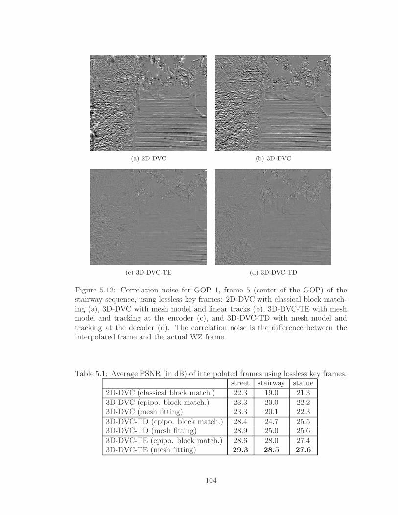
(a) 2D-DVC (b) 3D-DVC

(c) 3D-DVC-TE (d) 3D-DVC-TD

Figure 5.12: Correlation noise for GOP 1, frame 5 (center of the GOP) of thestairway sequence, using lossless key frames: 2D-DVC with classical block match-ing (a), 3D-DVC with mesh model and linear tracks (b), 3D-DVC-TE with meshmodel and tracking at the encoder (c), and 3D-DVC-TD with mesh model andtracking at the decoder (d). The correlation noise is the difference between theinterpolated frame and the actual WZ frame.

Table 5.1: Average PSNR (in dB) of interpolated frames using lossless key frames.street stairway statue

2D-DVC (classical block match.) 22.3 19.0 21.33D-DVC (epipo. block match.) 23.3 20.0 22.23D-DVC (mesh fitting) 23.3 20.1 22.33D-DVC-TD (epipo. block match.) 28.4 24.7 25.53D-DVC-TD (mesh fitting) 28.9 25.0 25.63D-DVC-TE (epipo. block match.) 28.6 28.0 27.43D-DVC-TE (mesh fitting) 29.3 28.5 27.6

104

5 10 15 20 25 30 35 40 45 5020

25

30

35

40

PS

NR

(dB

) ����

����

����

����

������� ��

Figure 5.13: PSNR of key frames and interpolated frames of the street sequenceusing 3D-DVC-TE with mesh fitting on lossy key frames. Peaks correspond to keyframes.

frame has (352/8)×(288/8) = 1584 blocks. On the other hand, the average number

of tracks is 128. Therefore, the complexity of the proposed tracking is only 8% of

a 2D BBMC.

Figure 5.13 shows the robustness of the proposed frame interpolation to quan-

tization noise, the quality of the interpolated frames degrading gracefully as the

bitrate is decreased. In the context of quantization, a larger quantization step size

decreases both the bitrate and the PSNR. However, it is not the case with frame in-

terpolation: a larger bitrate does not necessarily imply a larger PSNR. This figure

also shows that the PSNR of interpolated frames actually decreases more slowly

than that of key frames. Since quantization reduces the high-frequency content

of the key frames, it reduces the impact of interpolation misalignments. It also

reduces the impact of the low-pass effects of warping, both spatial and temporal.

The PSNR of interpolated frames has a ceiling value at about 30 dB. It is

quickly attained as the QP of key frames is decreased: this PSNR is about the

same whether key frames are losslessly encoded or quantized at QP = 26. In terms

of bitrate allocation, it means that in order to reach higher PSNR, more bits need

to be spent on parity bits.

Finally, although the objective quality strongly peaks at key frames, the sub-

jective quality is nearly constant, as shown in Figure 5.14. Both sources of errors,

105

(a) Frame 1 (PSNR: 36.5dB)

(b) Frame 5 (PSNR: 28.4dB)

Figure 5.14: Variation of the subjective quality at QP = 26 between a key frame(frame 1) and an interpolated frame (frame 5). In spite of a PSNR drop of 8.1 dB,both frames have a similar subjective quality.

misalignments and low-pass effects, are barely noticeable. This does not mean,

however, that they are not a limiting factor of the codec overall performances

because parity bits correct objective errors, not subjective ones.

5.5.3 Frame interpolation with tracking at the decoder(3D-DVC-TD)

Figures 5.11 and 5.12 show that point tracking at the decoder is also able to

greatly reduce misalignments and to consistently outperform 2D-DVC and 3D-

DVC. PSNR values obtained by 3D-DVC-TD are nearly constant inside each GOP

on the street sequence. The superiority of tracking at the encoder (3D-DVC-TE) is

in part due to the possibility of inserting new key frames and restarting tracking in

106

case of difficult motions. Like in the 3D-DVC-TE case, overheads are also limited.

An average of 176 feature points are detected at the encoder, which leads to a

bitrate overhead of 0.02 b/pixel. The complexity overhead is similar to the one of

intracoding.

5.5.4 Rate-distortion performances

Figure 5.15 compares the rate-distortion performances of the proposed mesh-based

codecs with version JM 9.5 of the H.264/AVC reference software and the 2D-DVC

software presented in [98]. The three proposed 3D codecs only differ from this

2D-DVC software by their side information generation. The 2D DVC software has

GOPs I-WZ-I, while H.264/AVC is tested in three modes: pure intra, inter-IPPP

with motion search, and IPPP with null motion vectors.

The 3D codecs with alignment (3D-DVC-TD and 3D-DVC-TE) strongly out-

perform the 3D codec without alignment (3D-DVC), confirming the need for precise

motion alignment. Compared to 2D-DVC, 3D-DVC-TE is superior over the whole

range of bitrates on all sequences while 3D-DVC-TD is superior on the street se-

quence over the whole range of bitrates, on the stairway sequence up to 990 kb/s

and on the statue sequence up to 740 kb/s. Note, however, that this RD gain

was achieved at the expense of the generality of the codec, 2D-DVC being able to

handle sequences with generic 2D motions.

Finally, compared to H.264/AVC, both 3D codecs with alignment outperform

intracoding and underperform intercoding with motion search. Since 3D-DVC-TE

benefits from limited interframe information at the encoder, it is also compared

to intercoding without motion search. The 3D codec is superior for bitrates up to

890 kb/s on the street sequence, over the whole range of bitrates on the stairway

sequence, and up to 1.4 Mb/s on the statue sequence.

107

0 0.5 1 1.520

22

24

26

28

30

32

34

36

Total rate (Mb/s)

PS

NR

(dB

)

0 0.5 1 1.520

22

24

26

28

30

32

34

36

Total rate (Mb/s)

�������������

���������

��������� ��������

���������

������

���������

���������

0 0.5 1 1.520

22

24

26

28

30

32

34

36

PS

NR

(dB

)

Total rate (Mb/s)

Figure 5.15: Rate-distortion curves for H.264/AVC intra, H.264/AVC inter-IPPPwith null motion vectors, H.264/AVC inter-IPPP, 2D-DVC I-WZ-I, and the threeproposed 3D codecs (top left: street, top right: stairway, bottom: statue).

108

5.6 Conclusion

In this chapter, we have explored the benefits of the SfM paradigm for distributed

coding of videos of static scenes captured by a moving camera. The SfM approach

allows introducing scene geometrical constraints in the side information generation

process. We have first developed two frame interpolation methods based either on

block matching along epipolar lines or 3D-mesh fitting. These techniques make use

of a robust feature-point matching algorithm leading to semidense correspondences

between pairs of consecutive key frames. The resulting interpolated motion fields

show a reduced number of outliers compared with motion fields obtained from 2D

block-based matching and interpolation techniques. It has been observed that this

property does not translate into significant side information PSNR gains, because

of misalignments problems betweens the side information and the Wyner-Ziv en-

coded frames. This limitation has been overcome by estimating the intermediate

projection matrices from point tracks obtained either at the encoder or at the

decoder, instead of interpolating it. It has led to major side information PSNR

improvements with only limited overheads, both in terms of bitrate and encoder

complexity. As an additional feature, point tracking at the encoder enables a rough

estimation of the video motion content, which is sufficient to select the key frames

adaptively. The RD performance of the resulting three DVC schemes has been

assessed against several techniques, showing the benefits of the 3D model based

interpolation methods augmented with feature point tracking for the type of ap-

plication and content considered. Further studies would be needed to extend the

proposed frame interpolation technique to videos with more generic motion fields

and to assess such methods against solutions in which limited motion search would

be considered at the encoder.

109

5.7 Acknowledgments

This work has been done in collaboration with Christine Guillemot and Luce

Morin, INRIA, Rennes, France. It has been partly funded by the European Com-

mission in the context of the network of excellence SIMILAR and of the IST-

Discover project. The author is thankful to the IST development team for its

original work on the IST-WZ codec [98] and the Discover software team for the

improvements they brought.

110

CHAPTER 6

CONCLUSION

In this dissertation, we have studied issues related to free-view 3D-video, and in

particular issues of 3D scene reconstruction, compression, and rendering. We have

presented four main contributions. First, we have presented a novel algorithm

which performs surface reconstruction from planar arrays of cameras and gener-

ates dense depth maps with multiple values per pixel. Second, we have introduced

a novel codec for the static depth-image-based representation, which jointly es-

timates and encodes the unknown depth map from multiple views using a novel

rate-distortion optimization scheme. Third, we have proposed a second novel codec

for the static depth-image-based representation, which relies on a shape-adaptive

wavelet transform and an explicit representation of the locations of major depth

edges to achieve major rate-distortion gains. Finally, we have proposed a novel al-

gorithm to extract the side information in the context of distributed video coding

of 3D scenes.

Several issues remain to be solved to obtain a telepresence system offering at

the same time realism, stereopsis, mobility, and interactivity. The efficient com-

pression of the depth maps with multiple values per pixels obtained in Chapter 2 is

still an open problem, which might be addressed by an extension of image-coding

techniques based on geometric wavelets [112]. Moreover, little is still known on

the generalization of 3D reconstruction and compression from static to dynamic

scenes. Finally, efficient approximations of the algorithms proposed here also need

to be designed to meet the constraints of real-time applications.

111

APPENDIX A

FIXING THE PROJECTIVEBASIS

During the nonlinear optimization of projection matrix P(1), the projective basis

is fixed by setting P(0) = [I 0] and choosing two points {X(1), X(2)} and their

projections. We would like to obtain a minimum parameterization of P(1). The

two points induce six constraints on P(1), four of which are independent. Each

point is associated with an equation of the form λ(1)x(1) = P(1)X. Using the third

component to solve for λ(1), we obtain x(1)P(1)3: X = P

(1)1: X and y(1)P

(1)3: X = P

(1)2: X.

These equations can be rewritten as AP(1)s = 0 where A is defined as

A ,

X⊺(1) 0 −x(1)(1)X(1)

0 X⊺(1) −y(1)(1)X(1)

X⊺(2) 0 −x(1)(2)X(2)

0 X⊺(2) −y(1)(2)X(2)

. (A.1)

Taking the SVD of A gives

A = U

S 0

0 0

V⊺

W⊺

, (A.2)

where S,V, and W are three matrices. Therefore, the projection matrices P(1)

can be parameterized by a vector r such that P(1)s =√

3Wr, where the factor√

3

was introduced so that a unit-norm vector r corresponds to ‖P(1)‖22 = 3.

112

APPENDIX B

BUNDLE ADJUSTMENT

The bundle adjustment problem given by Equation 5.5 is solved using an alternated

reweighted linear least square approach [103]. First, the denominators are factored

out and treated as constant weights, only updated at the end of each iteration.

These weights, denoted κ(1)(i), are defined as

κ(1)(i) ,

∣

∣

∣

[

λ(0)(i) x(0)⊺(i) 1]

P(1)s9:12

∣

∣

∣

−1

(B.1)

and initialized to 1. The problem then becomes biquadratic in its parameters:

min{λ(0)(i)},P(1)s

∑

i

κ2(i)(

(

[

λ(0)(i) x(0)⊺(i) 1]

(

x(1)(i)P(1)s9:12 −P

(1)s1:4

))2

+(

[

λ(0)(i) x(0)⊺(i) 1]

(

y(1)(i)P(1)s9:12 −P

(1)s5:8

))2 )

such that

P(1)s =√

3Wr

‖r‖22 = 1

(B.2)

which is solved by alternatively fixing either the projective depths {λ(0)} or the

camera parameters P(1)s and minimizing over the free parameters.

When the projective depths {λ(0)} are fixed, the problem is equivalent to finding

the unit-norm vector r that minimizes the squared norm of Ar, where matrix A is

113

obtained by stacking together sub-matrices of the form

√3κ

−λ(0)x(0)⊺ −1 0 0 x(1)λ(0)x(0)⊺ x(1)

0 0 −λ(0)x(0)⊺ −1 y(1)λ(0)x(0)⊺ y(1)

W. (B.3)

The solution is obtained by taking the SVD of matrix A and choosing the vector

associated with the smallest singular-value.

When the camera parameters P(1)s are fixed, the problem is unconstrained and

its Hessian is diagonal. Taking the derivative with regard to a particular {λ(0)}

and setting it to 0 leads to the solution

λ(0) = −a⊺b

a⊺awhere

a ,

x(1)P(1)s ⊺

9:11 −P(1)s ⊺

1:3

y(1)P(1)s ⊺

9:11 −P(1)s ⊺

5:7

x(0) ,

b ,

x(1)P(1)s12 −P

(1)s4

y(1)P(1)s12 −P

(1)s8

.

(B.4)

114

APPENDIX C

PUBLICATIONS

C.1 Journals

1. M. Maitre, Y. Shinagawa, and M. N. Do, “Joint estimation and encoding

of scalable depth-image-based representations for free-viewpoint rendering,”

IEEE Transactions on Image Processing, submitted for publication.

2. M. Maitre, C. Guillemot, and L. Morin, “3D model-based frame interpolation

for distributed video coding,” IEEE Transactions on Image Processing, vol.

16, pp. 1246-1257, 2007.

3. G. Guetat, M. Maitre, L. Joly, S.-L. Lai, T. Lee, and Y. Shinagawa, “Au-

tomatic 3-D grayscale volume matching and shape analysis,” IEEE Trans-

actions on Information Technology in Biomedicine, vol. 10, pp. 362-376,

2006.

C.2 Conferences

1. M. Maitre and M. N. Do, “Joint encoding of the depth image based represen-

tation using shape-adaptive wavelets,” in ICIP, submitted for publication.

2. M. Maitre, Y. Shinagawa, and M. N. Do, “Symmetric multi-view stereo re-

construction from planar camera arrays,” in CVPR, submitted for publica-

tion.

115

3. Y. Chen, M. Maitre, and F. Tong, “Transparent layer separation for dual

energy imaging,” in ICIP, submitted for publication.

4. M. Maitre, Y. Chen, and F. Tong, “High-dynamic-range compression using

a fast multiscale optimization,” in ICASSP, to appear.

5. M. Maitre, Y. Shinagawa, and M. N. Do, “Rate-distortion optimal depth

maps in the wavelet domain for free-viewpoint rendering,” in ICIP, 2007.

6. M. Maitre, C. Guillemot, and L. Morin, “3D scene modeling for distributed

video coding,” in ICIP, 2006.

C.3 Research Reports

1. Y. Chen, M. Maitre, and F. Tong, “High-dynamic-range compression us-

ing a fast mean-field gradient remapping with artifact correction,” Siemens

Corporate Research Tech. Rep., 2007.

2. M. Maitre, C. Guillemot, and L. Morin, “Reliable optical-flow estimation for

distributed video coding,” Irisa Res. Rep., 2007.

3. M. Maitre, V. Kindratenko, and Y. Shinagawa, “Laser-assisted 3D scene

reconstruction technique,” NCSA Tech. Rep., 2005.

4. M. Maitre, V. Kindratenko, and Y. Shinagawa, “Passive 3D scene recon-

struction technique,” NCSA Tech. Rep., 2005.

116

REFERENCES

[1] F. Herbert, Dune. Philadelphia, PA: Chilton Books, 1965.

[2] Jamiroquai, Travelling Without Moving. Sony, B000002BSG, 1997.

[3] J. Battelle, “HP’s HALO: Now this is telepresence,” May 2007. [Online].Available: http://battellemedia.com/archives/003632.php.

[4] “Wired travel guide: Second life,” 2006. [Online]. Available: http://www.wired.com/wired/archive/14.10/sloverview.html.

[5] M. Kanellos, “Philips: 3D-TV to appear in 2008,” 2006. [Online].Available: http://news.com.com/Philips+3D+TV+to+appear+in+2008/2100-1041 3-6022254.html.

[6] NVIDIA, “3D stereo,” NVIDIA, Santa Clara, CA, Technical Brief TB-00252-001 v02, 2003.

[7] T. Kanade, P. Rander, and P. Narayanan, “Virtualized reality: Constructingvirtual world from real scenes,” IEEE Multimedia, vol. 4, no. 1, pp. 34–46,1997.

[8] C. Zitnick, S. Kang, M. Uyttendaele, S. Winder, and R. Szeliski, “High-quality video view interpolation using a layered representation,” in Proc.SIGGRAPH, 2004, pp. 600–608.

[9] M. Magnor, P. Ramanathan, and B. Girod, “Multi-view coding for image-based rendering using 3-D scene geometry,” IEEE Trans. on Circuits andSys. for Video Tech., vol. 13, no. 11, pp. 1092–1106, 2003.

[10] A. Smolic and P. Kauff, “Interactive 3-D video representation and coding,”Proc. of the IEEE, vol. 93, no. 1, pp. 98–110, 2005.

[11] E. Adelson and J. Bergen, “The plenoptic function and the elements of earlyvision,” in Computational Models of Visual Processing, M. S. Landy andJ. A. Movshon, Eds. Cambridge, MA: MIT Press, 1991, pp. 3–20.

[12] D. A. Forsyth and J. Ponce, Computer Vision: A Modern Approach.Lebanon, IN: Prentice Hall, 2002.

117

[13] B. K. P. Horn, Robot Vision. Cambridge, MA: MIT Press, 1986.

[14] R. Hartley and A. Zisserman, Multiple View Geometry in Computer Vision.Cambridge, UK: Cambridge University Press, 2000.

[15] O. Faugeras and Q.-T. Luong, The Geometry of Multiple Images.Cambridge, MA: MIT Press, 2001.

[16] Y. Ma, S. Soatto, J. Kosecka, and S. Sastry, An invitation to 3D vision.New York, NY: Springer-Verlag, 2004.

[17] T. Cover and J. Thomas, Elements of Information Theory. Hoboken, NJ:John Wiley and Sons Ltd., 1991.

[18] Mallat, A Wavelet Tour of Signal Processing. Burlington, MA: AcademicPress, 1999.

[19] D. Taubman and M. Marcellin, JPEG2000: Image Compression Fundamen-tals, Standards and Practice. New York, NY: Springer-Verlag, 2001.

[20] Y. Q. Shi and H. Sun, Image and Video Compression for Multimedia Engi-neering. Boca Raton, FL: CRC Press, 1999.

[21] V. Bhaskaran and K. Konstantinides., Image and Video Compression Stan-dards: Algorithms and Architectures. Boston, MA: Kluwer Academic Pub-lishers, 1997.

[22] M. Pharr and G. Humphreys, Physically Based Rendering: From Theory toImplementation. San Fransisco, CA: Morgan Kaufmann, 2004.

[23] G. Wolberg, Digital Image Warping. Piscataway, NJ: IEEE Press, 1994.

[24] H.-Y. Shum, S.-C. Chan, and S. B. Kang, Image-Based Rendering. NewYork, NY: Springer-Verlag, 2007.

[25] D. Scharstein and R. Szeliski, “A taxonomy and evaluation of densetwo-frame stereo correspondence algorithms,” Int. J. of Comp. Vis., vol. 47,no. 1–3, pp. 7–42, 2002.

[26] J. W. Shade, S. J. Gortler, L.-W. He, and R. Szeliski, “Layered depthimages,” in Proc. SIGGRAPH, 1998, pp. 231–242.

[27] X. Gu, S. J. Gortler, and H. Hoppe, “Geometry images,” in Proc. SIG-GRAPH, 2002, pp. 355–361.

[28] S. Seitz, B. Curless, J. Diebel, D. Scharstein, and R. Szeliski, “A compari-son and evaluation of multi-view stereo reconstruction algorithms,” in Proc.CVPR, 2006, pp. 519–528.

118

[29] G. Vogiatzis, C. C. H. Esteban, P. H. S. Torr, and R. Cipolla, “Multiviewstereo via volumetric graph-cuts and occlusion robust photo-consistency,”IEEE Trans. on PAMI, vol. 29, pp. 2241–2246, 2007.

[30] J. Sun, Y. Li, S. Kang, and H. Shum, “Symmetric stereo matching for oc-clusion handling,” in Proc. CVPR, 2005, pp. 399–406.

[31] Y. Deng, Q. Yang, X. Lin, and X. Tang, “Stereo correspondence with occlu-sion handling in a symmetric patch-based graph-cuts model,” IEEE Trans.on PAMI, vol. 29, pp. 1068–1079, 2007.

[32] R. I. Hartley, “Theory and practice of projective rectification,” Int. J. ofComp. Vis., vol. 35, pp. 115–127, 1999.

[33] A. Fusiello, E. Trucco, and A. Verri, “A compact algorithm for rectificationof stereo pairs,” Machine Vis. and Appli., vol. 12, pp. 16–22, 2000.

[34] N. Ayache and F. Lustman, “Trinocular stereovision for robotics,” IEEETrans. on PAMI, vol. 13, pp. 73–85, 1991.

[35] C. Sun, “Uncalibrated three-view image rectification,” Im. and Vis. Comp.,vol. 21, no. 3, pp. 259–269, 2003.

[36] Y. Wei and L. Quan, “Asymmetrical occlusion handling using graph cut formulti-view stereo,” in Proc. CVPR, 2005, pp. 902–909.

[37] S. B. Kang, R. Szeliski, and J. Chai, “Handling occlusions in dense multi-view stereo,” in Proc. CVPR, 2001, pp. 103–110.

[38] M.-A. Drouin, M. Trudeau, and S. Roy, “Geo-consistency for wide multi-camera stereo,” in Proc. CVPR, 2005, pp. 351–358.

[39] M. Goesele, B. Curless, and S. M. Seitz, “Multi-view stereo revisited,” inProc. CVPR, 2006, pp. 2402–2409.

[40] P. Gargallo and P. Sturm, “Bayesian 3D modeling from images using multipledepth maps,” in Proc. CVPR, 2005, pp. 885–891.

[41] C. L. Zitnick and S. B. Kang, “Stereo for image-based rendering using imageover-segmentation,” Int. J. of Comp. Vis., vol. 75, pp. 49–65, 2007.

[42] M. Jaesik, M. Powell, and K. W. Bowyer, “Automated performance evalu-ation of range image segmentation algorithms,” IEEE Trans. on Sys., Manand Cyber., vol. 34, pp. 263–271, 2004.

[43] H.-Y. Shum, J. Sun, S. Yamazaki, Y. Li, and C.-K. Tang, “Pop-up light field:An interactive image-based modeling and rendering system,” ACM Trans.on Graphics, vol. 23, pp. 143–162, 2004.

119

[44] C. Zhang and T. Chen, “View-dependent non-uniform sampling for image-based rendering,” in Proc. ICIP, 2004, pp. 2471–2474.

[45] L. Vincent and P. Soille, “Watersheds in digital spaces: An efficient algorithmbased on immersion simulations,” IEEE Trans. on PAMI, vol. 13, pp. 583–598, 1991.

[46] V. Kolmogorov and R. Zabih, “Multi-camera scene reconstruction via graphcuts,” in Proc. ECCV, 2002, pp. 8–40.

[47] C. Fehn, R. Barre, and R. S. Pastoor, “Interactive 3-D TV – concepts andkey technologies,” Proc. of the IEEE, vol. 94, no. 3, pp. 524–538, 2006.

[48] W. Matusik and H. Pfister, “3D-TV: A scalable system for real-time ac-quisition, transmission, and autostereoscopic display,” in Proc. SIGGRAPH,2004, pp. 814–824.

[49] H.-Y. Shum, S. B. Kang, and S.-C. Chan, “Survey of image-based represen-tations and compression techniques,” IEEE Trans. on Circuits and Sys. forVideo Tech., vol. 13, pp. 1020–1037, 2003.

[50] S.-C. Chan, K.-T. Ng, Z.-F. Gan, K.-L. Chan, and H.-Y. Shum, “The plenop-tic video,” IEEE Trans. on Circuits and Sys. for Video Tech., vol. 15, no. 12,pp. 1650–1659, 2005.

[51] L. Levkovich-Maslyuk, A. Ignatenko, A. Zhirkov, A. Konushin, I. K. Park,M. Han, and Y. Bayakovski, “Depth image-based representation and com-pression for static and animated 3-D objects,” IEEE Trans. on Circuits andSys. for Video Tech., vol. 14, pp. 1032–1045, 2004.

[52] J. Oh, Y.-S. Choi, R.-H. Park, J. Kim, T. Kim, and H. Jung, “Trinocularstereo sequence coding based on MPEG-2,” IEEE Trans. on Circuits andSys. for Video Tech., vol. 15, no. 3, pp. 425–429, 2005.

[53] R.-S. Wang and Y. Wang, “Multiview video sequence analysis, compression,and virtual viewpoint synthesis,” IEEE Trans. on Circuits and Sys. for VideoTech., vol. 10, pp. 397–410, 2000.

[54] R. Balter, P. Gioia, and L. Morin, “Scalable and efficient coding using 3Dmodeling,” IEEE Trans. on Multimedia, vol. 8, pp. 1147–1155, 2006.

[55] A. Ortega and K. Ramchandran, “Rate distortion methods in image andvideo compression,” IEEE Signal Proc. Mag., vol. 15, pp. 23–50, 1998.

[56] P. Ramanathan and B. Girod, “Rate-distortion analysis for light field codingand streaming,” EURASIP Sig. Proc.: Im. Com., vol. 21, pp. 462–475, 2006.

120

[57] J. Park and H. Park, “A mesh-based disparity representation method forview interpolation and stereo image compression,” IEEE Trans. on Im.Proc., vol. 15, pp. 1751–1762, 2006.

[58] D. P. Bertsekas, Dynamic Programming and Optimal Control. Nashua,NH: Athena Scientific, 2005.

[59] D. Tzovaras and M. G. Strintzis, “Motion and disparity field estimation usingrate-distortion optimization,” IEEE Trans. on Circuits and Sys. for VideoTech., vol. 8, pp. 171–180, 1998.

[60] J. Ellinas and M. Sangriotis, “Stereo video coding based on quad-tree decom-position of B-P frames by motion and disparity interpolation,” IEE Proc.-Vis. Im. Sig. Proc., vol. 152, no. 5, pp. 639–647, 2005.

[61] G. J. Sullivan and R. L. Baker, “Efficient quadtree coding of images andvideo,” IEEE Trans. on Im. Proc., vol. 3, pp. 327–331, 1994.

[62] G. Sullivan and T. Wiegand, “Video compression - from concepts to theH.264/AVC standard,” Proc. of the IEEE, vol. 93, pp. 18–31, 2005.

[63] Y. Yang and S. S. Hemami, “Generalized rate-distortion optimization formotion-compensated video coders,” IEEE Trans. on Circuits and Sys. forVideo Tech., vol. 10, pp. 942–955, 2000.

[64] G. M. Schuster and A. K. Katsaggelos, “An optimal quadtree-based motionestimation and motion-compensated interpolation scheme for video compres-sion,” IEEE Trans. on Im. Proc., vol. 7, pp. 1505–1523, 1998.

[65] M. Woo, J. Neider, T. Davis, and D. Shreiner, OpenGL Programming Guide.Lebanon, IN: Addison Wesley, 1999.

[66] W. Press, B. Flannery, S. Teukolsky, and W. Vetterling, Numerical Recipesin C : The Art of Scientific Computing. Cambridge, UK: CambridgeUniversity Press, 1993.

[67] G. Sullivan and T. Wiegand, “Rate-distortion optimization for video com-pression,” IEEE Signal Proc. Mag., pp. 74–90, 1998.

[68] D. Luenberger, Linear and Nonlinear Programming. Boston, MA: KluwerAcademic Publishers, 2003.

[69] P. J. Burt and E. H. Adelson, “The Laplacian pyramid as a compact imagecode,” IEEE Trans. on Com., vol. COM-31, no. 4, pp. 532–540, 1983.

[70] F. R. Kschischang, B. J. Frey, and H.-A. Loeliger, “Factor graphs and thesum-product algorithm,” IEEE Trans. on Info. Theory, vol. 47, pp. 498–519,2001.

121

[71] P. Felzenszwalb and D. Huttenlocher, “Efficient belief propagation for earlyvision,” in Proc. CVPR, 2004, pp. 41–54.

[72] J. D. Oh and R.-H. Park, “Reconstruction of intermediate views from stereo-scopic images using disparity vectors estimated by the geometrical con-straint,” IEEE Trans. on Circuits and Sys. for Video Tech., vol. 16, pp.638–641, 2006.

[73] J. E. Fowler, “QccPack: An open-source software library for quantization,compression, and coding,” in Proc. of SPIE Appli. of Digital Im. Proc., 2000,pp. 294–301.

[74] Y. Morvan, D. Farin, and P. H. N. de With, “Depth-image compressionbased on an R-D optimized quadtree decomposition for the transmission ofmultiview images,” in Proc. ICIP, 2007, pp. 105–108.

[75] S. Li and W. Li, “Shape-adaptive discrete wavelet transforms for arbitrarilyshaped visual object coding,” IEEE Trans. on Circuits and Sys. for VideoTech., vol. 10, pp. 725–743, 2000.

[76] Y. K. Liu and B. Zalik, “An efficient chain code with Huffman coding,”Pattern Recog., vol. 38, pp. 553–557, 2005.

[77] M. Maitre, Y. Shinagawa, and M. N. Do, “Wavelet-based joint estimation andencoding of depth-image-based representations for free-viewpoint rendering,”IEEE Trans. on Im. Proc., submitted for publication.

[78] J. Slepian and J. Wolf, “Noiseless coding of correlated information sources,”IEEE Trans. on Info. Theory, vol. 19, no. 4, pp. 471–480, 1973.

[79] A. Wyner and J. Ziv, “The rate-distortion function for source coding withside information at the decoder,” IEEE Trans. on Info. Theory, vol. 22, no. 1,pp. 1–10, January 1976.

[80] S. Pradhan and K. Ramchandran, “Distributed source coding using syn-dromes (DISCUS): Design and construction,” IEEE Trans. on Info. Theory,vol. 49, no. 3, pp. 626–643, March 2003.

[81] A. Aaron and B. Girod, “Compression with side information using turbocodes,” in Proc. IEEE Int. Data Compression Conf., 2002, pp. 252–261.

[82] J. Garcia-Frias and Y. Zhao, “Compression of correlated binary sources usingturbo codes,” IEEE Comm. Letters, vol. 5, pp. 417–419, 2001.

[83] J. Garcia-Frias and Y. Zhao, “Data compression of unknown single and cor-related binary sources using punctured turbo codes,” in Proc. Allerton Conf.on Com., Contr. and Comput., 2001.

122

[84] J. Bajcsy and P. Mitran, “Coding for the Slepian-Wolf problem with turbocodes,” in Proc. IEEE Int. Global Com. Conf., 2001, pp. 1400–1404.

[85] A. D. Liveris, Z. Xiong, and C. N. Georghiades, “Compression of binarysources with side information at the decoder using LDPC codes,” IEEEComm. Letters, vol. 6, pp. 440–442, 2002.

[86] T. Tian, J. Garcia-Frias, and W. Zhong, “Compression of correlated sourcesusing LDPC codes,” in Proc. IEEE Int. Data Compression Conf., 2003, p.450.

[87] A. Aaron, R. Zhang, and B. Girod, “Wyner-Ziv coding of motion video,” inProc. Asilomar Conf. on Sig., Sys. and Comp., 2002, pp. 240–244.

[88] A. Aaron, S. Rane, R. Zhang, and B. Girod, “Wyner-Ziv coding for video:Applications to compression and error resilience,” in Proc. IEEE Int. DataCompression Conf., 2003, pp. 93–102.

[89] A. Aaron, S. Rane, E. Setton, and B. Girod, “Transform-domain Wyner-Zivcodec for video,” in Proc. SPIE Conf. on Visual Com. and Im. Proc., 2004,pp. 520–528.

[90] R. Puri and K. Ramchandran, “PRISM: A new robust video coding archi-tecture based on distributed compression principles,” in Proc. Allerton Conf.on Com., Contr. and Comput., 2002.

[91] R. Puri and K. Ramchandran, “PRISM: A new reversed multimedia codingparadigm,” in Proc. ICIP, 2003, pp. 617–620.

[92] R. Puri, A. Majumbar, P. Ishwar, and K. Ramchandran, “Distributed videocoding in wireless sensor networks,” Signal Proc., vol. 23, pp. 94–106, 2006.

[93] B. Girod, A. Aaron, S. Rane, and D. Rebollo-Monedero, “Distributed videocoding,” Proc. of the IEEE, vol. 93, no. 1, pp. 71–83, January 2005.

[94] P. Ishwar, V. Prabhakaran, and K. Ramchandran, “Towards a theory forvideo coding using distributed compression principles,” in Proc. ICIP, 2003,pp. 687–690.

[95] J. Repko and M. Pollefeys, “3D models from extended uncalibrated videosequences: Addressing key-frame selection and projective drift,” in Proc.3-D Digit. Imag. and Model., 2005, pp. 150–157.

[96] F. Galpin and L. Morin, “Sliding adjustment for 3D video representation,”EURASIP J. on Applied Signal Proc., vol. 2002, no. 10, pp. 1088–1101, 2002.

[97] J. Ascenso, C. Brites, and F. Pereira, “Content adaptive Wyner-Ziv videocoding driven by motion activity,” in Proc. ICIP, 2006, pp. 605–608.

123

[98] J. Ascenso, C. Brites, and F. Pereira, “Improving frame interpolation withspatial motion smoothing for pixel domain distributed video coding,” inEURASIP Conf. on Speech and Im. Proc., Multim. Com. and Serv., 2005.

[99] P. Torr and A. Zisserman, “Robust computation and parametrization ofmultiple view relations,” in Proc. ICCV, 1998, pp. 727–732.

[100] O. Chum, J. Matas, and J. Kittler, “Locally optimized RANSAC,” in Proc.of the 25th DAGM Symp., 2003, pp. 236–243.

[101] P. A. Beardsley, A. Zisserman, and D. W. Murray, “Sequential updating ofprojective and affine structure from motion,” Int. J. of Comp. Vis., vol. 23,pp. 235–259, 1997.

[102] B. Matei and P. Meer, “A general method for errors-in-variables problems incomputer vision,” in Proc. CVPR, 2000, pp. 18–25.

[103] A. Bartoli, “A unified framework for quasi-linear bundle adjustment,” inProc. ICPR, 2002, pp. 560–563.

[104] C. Harris and M. Stephens, “A combined corner and edge detector,” in Proc.Alvey Vision Conf., 1988, pp. 147–151.

[105] R. Duda, P. Hart, and D. Strok, Pattern Classification. Hoboken, NJ: JohnWiley and Sons Ltd., 2001.

[106] S. Birchfield and C. Tomasi, “Depth discontinuities by pixel-to-pixel stereo,”Int. J. of Comp. Vis., vol. 35, pp. 269–293, 1999.

[107] M. Berg, M. Kreveld, M. Overmars, and O. Schwarzkopf, ComputationalGeometry: Algorithms and Applications. New York, NY: Springer-Verlag,2000.

[108] R. Hartley, “Chirality,” Int. J. of Comp. Vis., vol. 26, no. 1, pp. 41–61, 1998.

[109] R. Hartley, “Lines and points in three views and the trifocal tensor,” Int. J.of Comp. Vis., vol. 22, no. 2, pp. 125–140, 1997.

[110] S. Boyd and L. Vandenberghe, Convex Optimization. Cambridge, UK:Cambridge University Press, 2004.

[111] C. Xu and J. L. Prince, “Snakes, shapes, and gradient vector flow,” IEEETrans. on Im. Proc., vol. 7, pp. 359–369, 1998.

[112] G. Peyre and S. Mallat, “Surface compression with geometric bandelets,” inProc. SIGGRAPH, 2005, pp. 601–608.

124

AUTHOR’S BIOGRAPHY

Matthieu Maitre is a Ph.D. candidate at the Department of Electrical and Com-

puter Engineering, University of Illinois at Urbana-Champaign (UIUC). He re-

ceived in 2002 his diplome d’ingenieur from the Ecole Nationale Superieure de

Telecommunications (ENST) and his M.S. from the UIUC. His research interests

include computer vision, image analysis, stereovision, and video compression.

125