2002 Paladino Encit

Paper CIT02-0070

MULTI-PHASE FLOW MODELLING IN DIFFERENTIAL PRESSURE FLOW METERS

Emilio E. PaladinoComputational Fluid Dynamics Laboratory Department of Mechanical Engineering Federal University Santa Catarina Florianopolis -SC Brazil. CEP [email protected]

Clovis R. MaliskaComputational Fluid Dynamics Laboratory Department of Mechanical Engineering Federal University Santa Catarina Florianopolis -SC Brazil. CEP [email protected]

Abstract. The accurate flow rate measurement of multi-phase flows is an important task in petroleum and petrochemical industry.Unlike the measurement of single phase flows using differential pressure meters, the multi-phase flow behavior poses difficulties forthe accurate measurement. This work examines the characteristics of the multi-phase flow in differential pressure flow meters such asVenturi meters. For this purpose the Two-Fluid model, based on an Eulerian - Eulerian approach for the multi-phase mixture, will beused and it will be focused on the study of dispersed flows. In differential pressure-type flow meters, the accuracy depends strongly onthe knowledge of the flow behavior, fundamentally about the relation between differential pressure and mean velocity of the flow. Formulti-phase flow these relations are not fully known, and there are several new variables affecting the flow, like void fraction, relativevelocity between phases (slip velocity), interfacial momentum transfer, etc.. Preliminary results obtained using the two fluid model arecompared with experimental values of velocities distributions and differential pressure across the Venturi.

Keywords:Flow Metering, Multiphase Flows, Multi-Fluid Model.

1. Introduction

Pipeline transport of multiphase mixtures is commonly encountered in the petroleum industry. Mixtures of oils, waterand gas produced from wells or condensate fractions flowing with gas in gas pipeline transport are common examples.In any measurement system, the continuous improvement of its accuracy is always a main goal but in some critical areaslike reservoir management, leak detection, and fiscal metering, the device accuracy plays an extremely important role. Infiscal metering the accuracy requirements are around 1%, since this may represent considerable loss of money.

Differential pressure flow meters are present in several measurement systems, as a single measurement device or aspart of more complex systems as, for example, in the one described by Mehdizadeh and Farchy, 1995, which encompassesa volumetric flow meter, two venturi tubes and a water cut meter. In this system, the two venturi meters are for measuringthe two velocities, one for each phase. Another system using a venturi tube as a velocity meter is the one describedby Boyer and Lemonnier, 1996, which include a venturi and a mixer to homogenize phase velocities. Whatever theapplication, venturi type flow meters are largely used in pipeline transport of hydrocarbons due to their simplicity, lowcost, robustness and maintainability. These characteristics are strongly required for field applications, specially in off-shore conditions.

In differential pressure-type flow meters, the accuracy of the measurement depends strongly on the knowledge ofthe flow behavior. The relation between the differential pressure and the mean flow velocity is affected by various flowparameters, like void fraction, relative velocity between phases (slip velocity), interfacial momentum transfer etc.

The main objective of this work is to present the application of a two dimensional two-fluid model for the study ofthe flow structure in bubbly regime within a vertical venturi. This work is part of a more broad study aimed to analyzenumerical and experimentally the flow structure of gas-liquid flows in differential pressure flow meter, as venturi tubesand orifice plates.

In this work we present three modelling approaches for calculating dispersed flows and few preliminary results ob-tained using the two-fluid and homogeneous models running the CFX4 CFD commercial code (User Reference Manual,1999). The results are compared with some experimental data in literature. The experimental facilities that will be usedin this work are briefly described but no tests were still carried out.

2. Mathematical modelling

In correlating pressure drop in multiphase flow meters, it is common to use the homogeneous model. This model issimilar to a single phase model, in the sense that it considers only one velocity field, but uses special fluid properties,

1

Proceedings of the ENCIT 2002, Caxambu - MG, Brazil - Paper CIT02-0070

called properties of the mixture, to represent the multiphase flow behavior. In this section we will present the mostcommon approaches for modelling two-phase dispersed flows and, following, some results obtained using the two-fluidand the homogeneous models compared with the experimental data available in the literature.

2.1. The two-fluid model

The two-fluid model considers one velocity field for each phase. Each phase is supposed to behave as a continuousmedia occupying the entire domain, where the amount of each phase present is given by the volumetric fraction. Thegoverning equations for this model are derived by averaging the local conservation equations for each phase, togetherwith their corresponding conservation equations at the interfaces,i.e., the jump conditions. The mass and momentumconservation equations for the two-fluid model are, therefore, given by,

∂

∂t(riρi) + ∇ · (riρiUi) = 0 (1)

∂

∂t(riρiUi) + ∇ · (ri(ρiUiUi −Ti + TTurb

i ) = −ri∇pi +

+(piI − pi)∇ri + MiI +NP∑j=1

(mijUj − mjiUi) + rif (2)

where the sub-indexi indicates the phase,MiI is the interface transport term,ri is the volumetric fraction of phasei andmji is the mass transferred from phasej to i. A full description of the derivation of these equations is presented by Drew,1983.

The term(piI −pi) contains the force due to the interfacial pressure distribution. In vertical flows this term representsthe buoyancy force as this force is given by pressure (hydrostatic) differences distribution at the interfaces. Actually, theinterfacial pressure of all phases is considered equal and the buoyancy force is calculated byFB = (ρliq − ρgas)Vbubbleg.It is assumed that the bulk pressure of all phases, in the presence of any flow disturbance, have instantaneous equalization.Therefore, the pressure of the mixture in all points (phases and interfaces) is the same. As this problem does not includephase transition, the term

∑NP

j=1(mijUj − mjiU) is also zero.For the continuous phase, ak − ε turbulence model was used, including the bubble induced turbulence through Sato

and Sekoguchi, 1975 model. For the dispersed phase, the viscous terms were neglected, since in the authors judgement,it is not available in the literature physically founded models for the stress tensor. Drew, 1983 shows that the effectiveviscosity of the dispersed phase can be obtained multiplying the effective viscosity of the continuous phase by the densityratio as,

µeffgas =

ρgas

ρliq· µeff

liq (3)

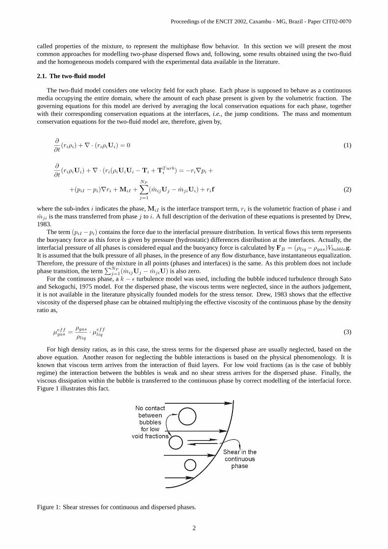
For high density ratios, as in this case, the stress terms for the dispersed phase are usually neglected, based on theabove equation. Another reason for neglecting the bubble interactions is based on the physical phenomenology. It isknown that viscous term arrives from the interaction of fluid layers. For low void fractions (as is the case of bubblyregime) the interaction between the bubbles is weak and no shear stress arrives for the dispersed phase. Finally, theviscous dissipation within the bubble is transferred to the continuous phase by correct modelling of the interfacial force.Figure 1 illustrates this fact.

Figure 1: Shear stresses for continuous and dispersed phases.

2


In the CFX4 code, the viscous terms in the dispersed phase are neglected by setting a very low viscosity (µ = 1e−20)and setting a slip condition at the wall boundaries for this phase.Then, the momentum balance for the dispersed phaseis given by the inertial, pressure, interfacial and body forces as is done in several one-dimensional models present in theliterature (Lewis and Davidson, 1985, Couët et al., 1991, Kowe et al., 1988, among others).

2.2. The homogeneous model

This simple model can be deduced from the more general two-fluid model by summing over all phases the conservationequations. The main disadvantage of this model is that it considers only one velocity field for all phases. For the problemwe are interested in,i.e., to predict multiphase flow field in geometries like venturis and orifice plates, where high localaccelerations are present generating high slip velocities, this assumption is no longer valid. The governing equations forthis model are similar to those for single phase flows, but uses special fluid properties representing the mixture behavior,as described above. The CFX4 code allows to calculate the volumetric fractions for each phase by solving individual massconservation equations and one momentum equation for all phases. These equations are

∂

∂t(riρi) + ∇ · (riρiUi) = 0 (4)

∂

∂t(ρmixU) + ∇ · ((ρmix(UU) −Tmix + TTurb

mix ) = −∇p + f (5)

Since the total mass flow rate is the sum of the individual mass flow rates of each phase, given by

ρmixUmix = ρliqrliqUliq + ρgasrgasUgas (6)

we obtain the mixture density as

ρmix = ρliqrliq + ρgasrgas (7)

This obviously considers that both velocities are equal, which is the main simplificative hypothesis of the homoge-neous model. Summing the momentum equations for each phase in the two-fluid model and considering again the equalityof the velocities, we obtain a viscosity for the mixture as

µmix = µliqrliq + µgasrgas (8)

This viscosity appears naturally when the phase velocities are considered equal. In order to improve this model,various other correlations for the viscosity are presented in the literature. In this work, the above model will be used whenwe refer to the homogeneous model.

The stress tensor for the mixture is calculated by the traditional approach, that is, proportional to the strain tensor,but using a mixture viscosity given by Eq. 8. For very fine dispersions, as oil in water emulsions, the hypothesis of thehomogeneity of velocities is valid and this model could be used. Care should be exercised, however, when the mixtureshows non-newtonian behavior. The velocity in the previous equations represents the velocity of the center of mass of themixture and is given by,

Umix =1

ρmix

NP∑i=1

riρiUi (9)

2.3. The three field model

This model presented by Kowe et al., 1988 and used by Boyer and Lemonnier, 1996 for the calculation of two phaseflows within venturi tubes considers the two-phase mixture as being composed by three fields as being,

• The bubbles occupying the volumeαV which velocity is,V

• The liquid displaced by bubble flowing with its velocity and occupying the volumeCMαV

• The intersticial liquid, which is the liquid flowing far from bubbles which volume isV −αV −CMαV and flowingwith the liquid velocity,U0.

3


Figure 2: Local interfacial force.

In all cases,V is the total volume occupied by the mixture andα is the void fraction. The virtual mass coefficient,CM represents the fraction of liquid, relative to the bubble volume, displaced by bubbles. Therefore, the liquid volumedisplaced by a bubble of volumeVb is CMVb. The mass of liquid contained in this volume is the so called virtual mass.

Therefore, this model considers that in the mass and momentum balances a parcel of liquid is displaced by bubbles,handling the virtual mass force in a more consistent form. As described in the next section, this force is given by therelative acceleration of the parcel of continuous phase displaced by the bubbles.

2.4. Interfacial forces

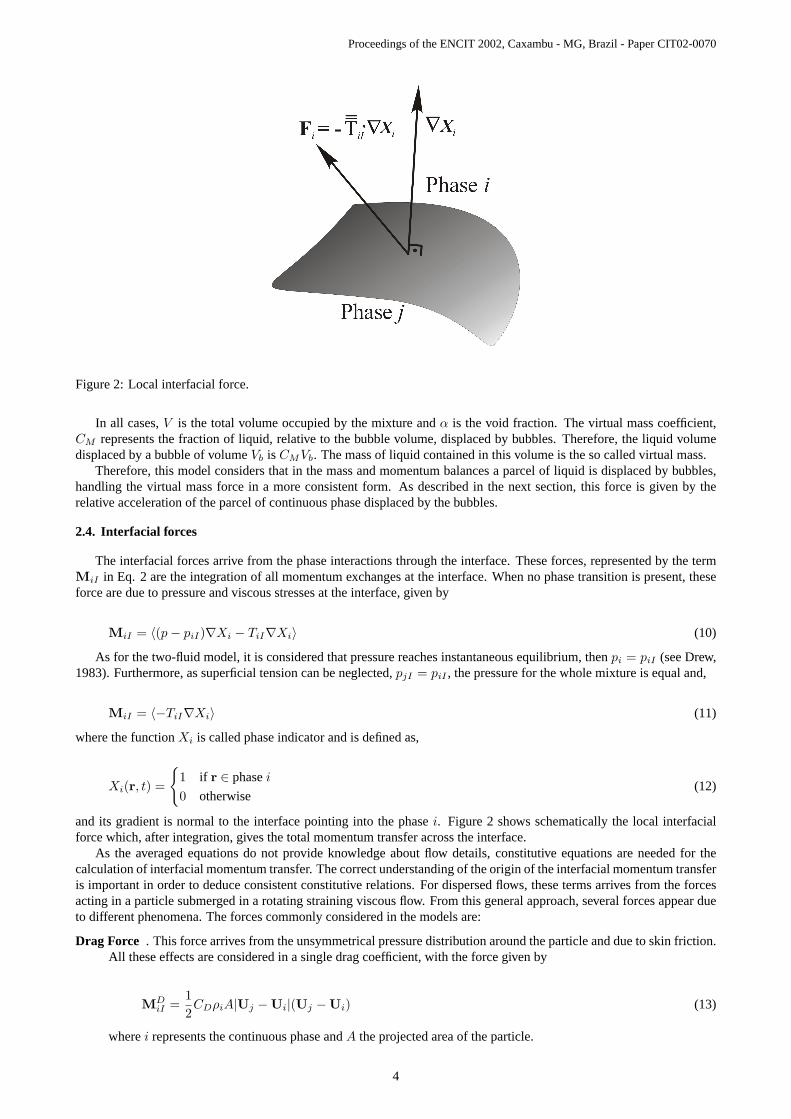
The interfacial forces arrive from the phase interactions through the interface. These forces, represented by the termMiI in Eq. 2 are the integration of all momentum exchanges at the interface. When no phase transition is present, theseforce are due to pressure and viscous stresses at the interface, given by

MiI = 〈(p − piI)∇Xi − TiI∇Xi〉 (10)

As for the two-fluid model, it is considered that pressure reaches instantaneous equilibrium, thenpi = piI (see Drew,1983). Furthermore, as superficial tension can be neglected,pjI = piI , the pressure for the whole mixture is equal and,

MiI = 〈−TiI∇Xi〉 (11)

where the functionXi is called phase indicator and is defined as,

Xi(r, t) =

{1 if r ∈ phasei

0 otherwise(12)

and its gradient is normal to the interface pointing into the phasei. Figure 2 shows schematically the local interfacialforce which, after integration, gives the total momentum transfer across the interface.

As the averaged equations do not provide knowledge about flow details, constitutive equations are needed for thecalculation of interfacial momentum transfer. The correct understanding of the origin of the interfacial momentum transferis important in order to deduce consistent constitutive relations. For dispersed flows, these terms arrives from the forcesacting in a particle submerged in a rotating straining viscous flow. From this general approach, several forces appear dueto different phenomena. The forces commonly considered in the models are:

Drag Force . This force arrives from the unsymmetrical pressure distribution around the particle and due to skin friction.All these effects are considered in a single drag coefficient, with the force given by

MDiI =

12CDρiA|Uj −Ui|(Uj −Ui) (13)

wherei represents the continuous phase andA the projected area of the particle.

4


Virtual Mass Force . This force is due to the relative acceleration between phases. It is known that when a particlepasses through a fluid at rest, a volume of fluid, proportional to the particle volume, is displaced and assumes theparticle velocity. The acceleration from the rest to the particle velocity (or from the continuous phase velocity tothe dispersed phase velocity, in the case of two-phase flows), originates a force given by,

MV MiI = ρirjCV M

(DjUj

Dt− DiUi

Dt

)(14)

whereCV M represents the fraction of the particle volume displaced from the continuous phase. For an infinitemediumCV M = 0.5, and this value can be used for low void fractions.

Lift Force . This force is perpendicular to the main flow and is originated by the vorticity of the continuous phase. It isgiven by,

MLiI = rjρiCL(Uj −Ui) · (U× ~ω) (15)

For more details about the physical significance of the virtual mass and lift forces, see, for example, Drew, 1983or Kowe et al., 1988. A detailed explanation about the origin of these forces and the mathematical treatment could beencountered in Drew and Lahey, 1987 and Drew and Lahey, 1990.

In this work, only the drag force has been considered. Although the non-drag forces represent a small fraction ofthe interfacial momentum transfer termMiI , for various applications (strong local accelerations is one example), theseforces can play an important role. As will be seen in the next section, neglecting the virtual mass force does not affectsignificantly the velocity fields, but can greatly underestimate the determination of the differential pressure, which is thefocus of this study.

Various models exist for the drag coefficient, depending on the local flow regime around the bubble. Here, it wasused a model based on a terminal bubble velocity, which takes into account the bubble deformation for high velocityregimes. An expression for the drag coefficient is obtaining invoking the equilibrium between buoyancy and drag forcesfor a bubble ascending in a quiescent liquid,

(ρliq − ρgas)g43πr3 = CDπr2 1

2ρliqU

2T (16)

therefore,

CD =83

gr∆ρ

ρliqU2T

(17)

whereUT is the terminal bubble rise velocity,g is the gravity acceleration anr is the bubble radius. In all cases, bubblemean diameter used were of 5 mm and terminal rise velocity of 0.2 m/s, givingCD = 1.63. Further studies are beingcarried out to investigate the influence of bubble diameter and break-up and coalescence on the differential pressure valuesand on the flow structure.

3. Results

The multidimensional multiphase CFX4 code was used for the solution of the mass and momentum equations. Thiscode solves the Navier-Stokes equations using the Finite Volume method and generalized coordinates. The code solvesthe mass and momentum equations using SIMPLE-C method for the pressure Velocity coupling and the IPSA-C method(see Karema and Lo, 1999 for a detailed description) for the interphase coupling.

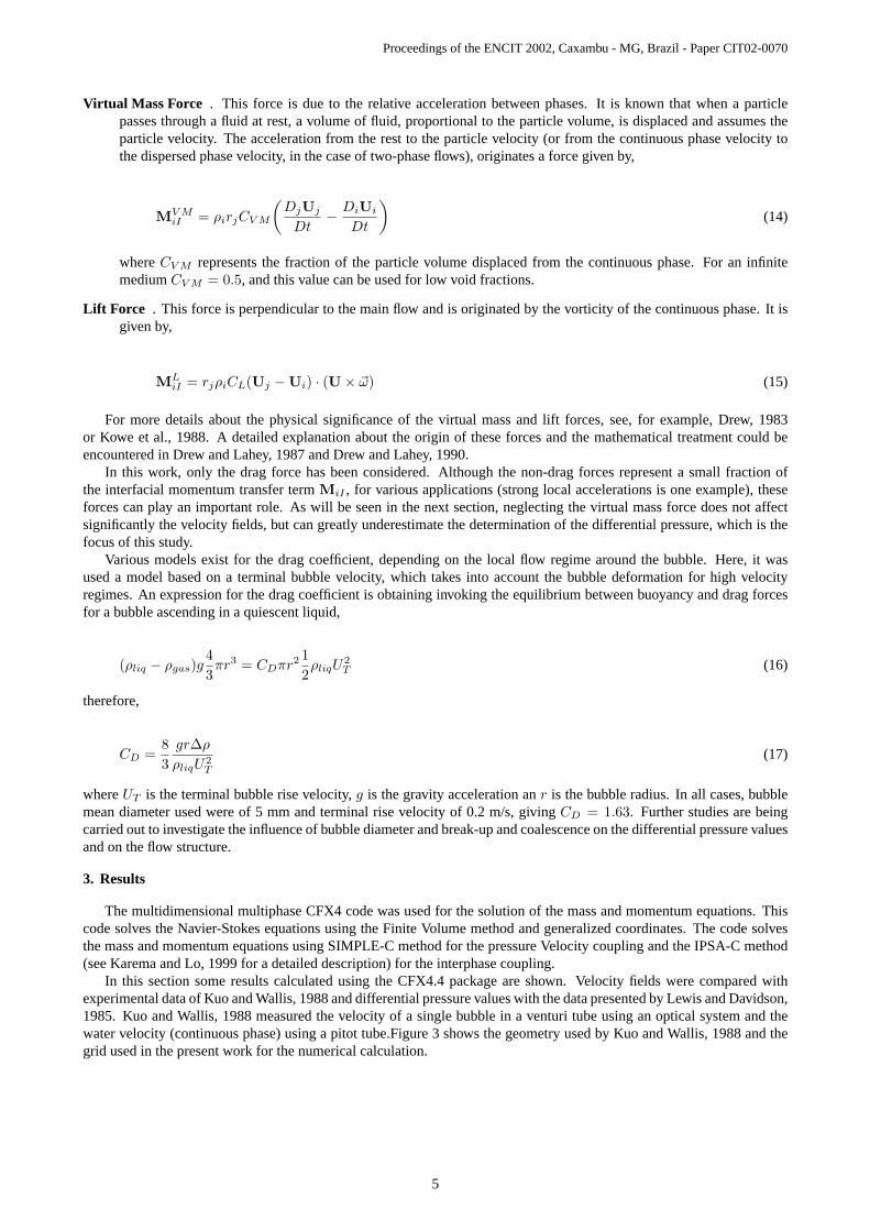
In this section some results calculated using the CFX4.4 package are shown. Velocity fields were compared withexperimental data of Kuo and Wallis, 1988 and differential pressure values with the data presented by Lewis and Davidson,1985. Kuo and Wallis, 1988 measured the velocity of a single bubble in a venturi tube using an optical system and thewater velocity (continuous phase) using a pitot tube.Figure 3 shows the geometry used by Kuo and Wallis, 1988 and thegrid used in the present work for the numerical calculation.

5


Figure 3: Geometry used by Kuo and Wallis, 1988 and computational grid used in this work.

The problem was treated as two-dimensional, using the symmetry condition at the centerline. Some tests were alsocarried out using a three dimensional geometry and no differences were found in terms of flow structure and velocitydistribution. The two-dimensional results obtained were averaged through the cross section of the venturi in order tocompare with one-dimensional results given by Kuo and Wallis, 1988. For a generic scalarφ, which could represent thevelocity components, pressure or void fraction, the average value at any point of the axial coordinate is

φ =1A

∫ Wall

CL

φdA (18)

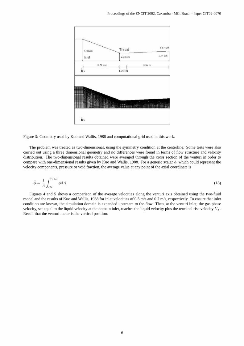
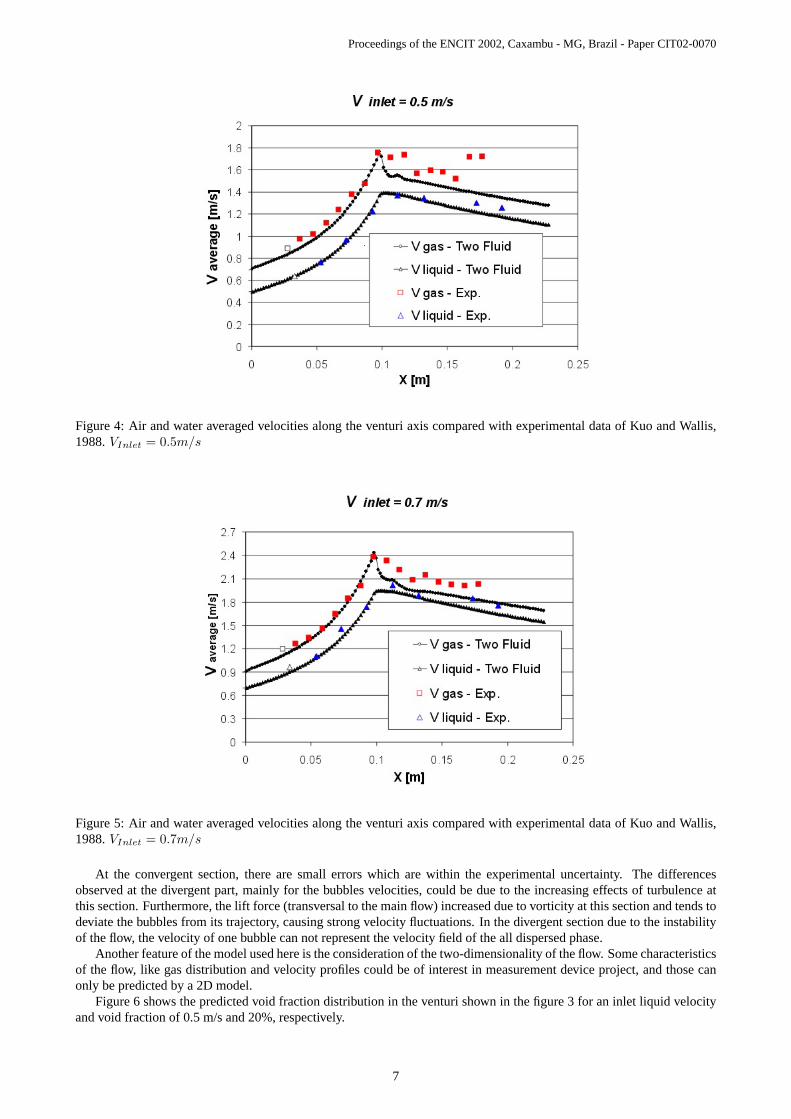
Figures 4 and 5 shows a comparison of the average velocities along the venturi axis obtained using the two-fluidmodel and the results of Kuo and Wallis, 1988 for inlet velocities of 0.5 m/s and 0.7 m/s, respectively. To ensure that inletcondition are known, the simulation domain is expanded upstream to the flow. Then, at the venturi inlet, the gas phasevelocity, set equal to the liquid velocity at the domain inlet, reaches the liquid velocity plus the terminal rise velocityUT .Recall that the venturi meter is the vertical position.

6


Figure 4: Air and water averaged velocities along the venturi axis compared with experimental data of Kuo and Wallis,1988.VInlet = 0.5m/s

Figure 5: Air and water averaged velocities along the venturi axis compared with experimental data of Kuo and Wallis,1988.VInlet = 0.7m/s

At the convergent section, there are small errors which are within the experimental uncertainty. The differencesobserved at the divergent part, mainly for the bubbles velocities, could be due to the increasing effects of turbulence atthis section. Furthermore, the lift force (transversal to the main flow) increased due to vorticity at this section and tends todeviate the bubbles from its trajectory, causing strong velocity fluctuations. In the divergent section due to the instabilityof the flow, the velocity of one bubble can not represent the velocity field of the all dispersed phase.

Another feature of the model used here is the consideration of the two-dimensionality of the flow. Some characteristicsof the flow, like gas distribution and velocity profiles could be of interest in measurement device project, and those canonly be predicted by a 2D model.

Figure 6 shows the predicted void fraction distribution in the venturi shown in the figure 3 for an inlet liquid velocityand void fraction of 0.5 m/s and 20%, respectively.

7


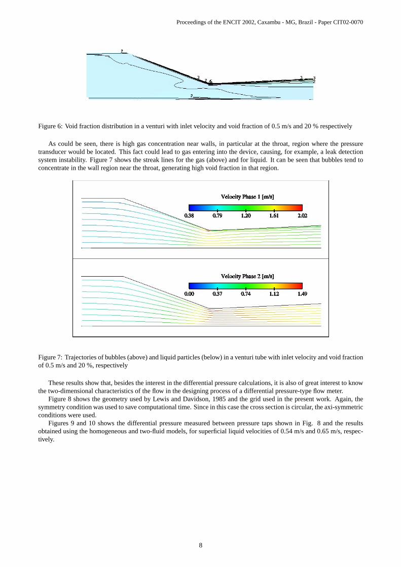
Figure 6: Void fraction distribution in a venturi with inlet velocity and void fraction of 0.5 m/s and 20 % respectively

As could be seen, there is high gas concentration near walls, in particular at the throat, region where the pressuretransducer would be located. This fact could lead to gas entering into the device, causing, for example, a leak detectionsystem instability. Figure 7 shows the streak lines for the gas (above) and for liquid. It can be seen that bubbles tend toconcentrate in the wall region near the throat, generating high void fraction in that region.

Figure 7: Trajectories of bubbles (above) and liquid particles (below) in a venturi tube with inlet velocity and void fractionof 0.5 m/s and 20 %, respectively

These results show that, besides the interest in the differential pressure calculations, it is also of great interest to knowthe two-dimensional characteristics of the flow in the designing process of a differential pressure-type flow meter.

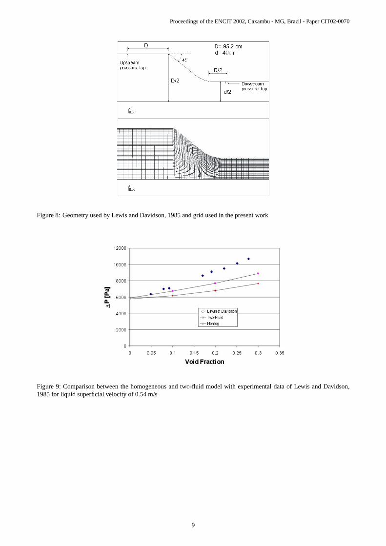
Figure 8 shows the geometry used by Lewis and Davidson, 1985 and the grid used in the present work. Again, thesymmetry condition was used to save computational time. Since in this case the cross section is circular, the axi-symmetricconditions were used.

Figures 9 and 10 shows the differential pressure measured between pressure taps shown in Fig. 8 and the resultsobtained using the homogeneous and two-fluid models, for superficial liquid velocities of 0.54 m/s and 0.65 m/s, respec-tively.

8


Figure 8: Geometry used by Lewis and Davidson, 1985 and grid used in the present work

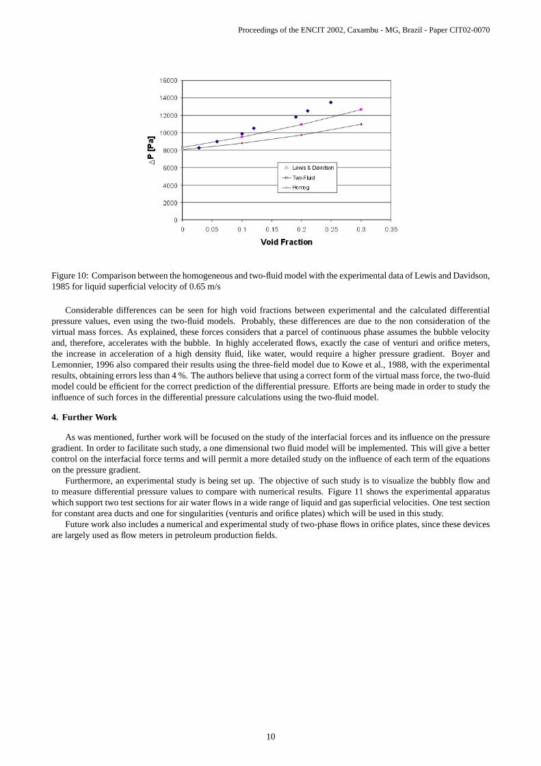
Figure 9: Comparison between the homogeneous and two-fluid model with experimental data of Lewis and Davidson,1985 for liquid superficial velocity of 0.54 m/s

9


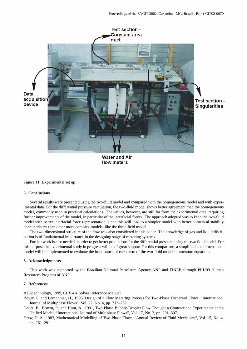
Figure 10: Comparison between the homogeneous and two-fluid model with the experimental data of Lewis and Davidson,1985 for liquid superficial velocity of 0.65 m/s

Considerable differences can be seen for high void fractions between experimental and the calculated differentialpressure values, even using the two-fluid models. Probably, these differences are due to the non consideration of thevirtual mass forces. As explained, these forces considers that a parcel of continuous phase assumes the bubble velocityand, therefore, accelerates with the bubble. In highly accelerated flows, exactly the case of venturi and orifice meters,the increase in acceleration of a high density fluid, like water, would require a higher pressure gradient. Boyer andLemonnier, 1996 also compared their results using the three-field model due to Kowe et al., 1988, with the experimentalresults, obtaining errors less than 4 %. The authors believe that using a correct form of the virtual mass force, the two-fluidmodel could be efficient for the correct prediction of the differential pressure. Efforts are being made in order to study theinfluence of such forces in the differential pressure calculations using the two-fluid model.

4. Further Work

As was mentioned, further work will be focused on the study of the interfacial forces and its influence on the pressuregradient. In order to facilitate such study, a one dimensional two fluid model will be implemented. This will give a bettercontrol on the interfacial force terms and will permit a more detailed study on the influence of each term of the equationson the pressure gradient.

Furthermore, an experimental study is being set up. The objective of such study is to visualize the bubbly flow andto measure differential pressure values to compare with numerical results. Figure 11 shows the experimental apparatuswhich support two test sections for air water flows in a wide range of liquid and gas superficial velocities. One test sectionfor constant area ducts and one for singularities (venturis and orifice plates) which will be used in this study.

Future work also includes a numerical and experimental study of two-phase flows in orifice plates, since these devicesare largely used as flow meters in petroleum production fields.

10


Figure 11: Experimental set up

5. Conclusions

Several results were presented using the two-fluid model and compared with the homogeneous model and with exper-imental data. For the differential pressure calculation, the two-fluid model shows better agreement than the homogeneousmodel, commonly used in practical calculations. The values, however, are still far from the experimental data, requiringfurther improvements of the model, in particular of the interfacial forces. The approach adopted was to keep the two-fluidmodel with better interfacial force representation, since this will lead to a simpler model with better numerical stabilitycharacteristics than other more complex models, like the three-field model.

The two-dimensional structure of the flow was also considered in this paper. The knowledge of gas and liquid distri-bution is of fundamental importance in the designing stage of metering systems.

Further work is also needed in order to get better predictions for the differential pressure, using the two fluid model. Forthis purpose the experimental study in progress will be of great support For this comparison, a simplified one dimensionalmodel will be implemented to evaluate the importance of each term of the two-fluid model momentum equations.

6. Acknowledgments

This work was supported by the Brazilian National Petroleum Agency-ANP and FINEP, through PRH09 HumanResources Program of ANP.

7. References

AEATechnology, 1999, CFX 4.4 Solver Reference Manual.Boyer, C. and Lemonnier, H., 1996, Design of a Flow Metering Process for Two-Phase Dispersed Flows, “International

Journal of Multiphase Flows”, Vol. 22, No. 4, pp. 713–732.Couët, B., Brown, P., and Hunt, A., 1991, Two Phase Bubbly-Droplet Flow Thought a Contraction: Experiments and a

Unified Model, “International Journal of Multiphase Flows”, Vol. 17, No. 3, pp. 291–307.Drew, D. A., 1983, Mathematical Modelling of Two-Phase Flows, “Annual Review of Fluid Mechanics”, Vol. 15, No. 4,

pp. 261–291.

11


Drew, D. A. and Lahey, R. T., 1987, The Virtual Mass and Lift Force on a Sphere in Rotating and Straining Inviscid Flow,“International Journal of Multiphase Flows”, Vol. 13, No. 1, pp. 113–121.

Drew, D. A. and Lahey, R. T., 1990, Some Supplemental Analysis Concerning The Virtual Mass and Lift Force on aSphere in Rotating and Straining Inviscid Flow, “International Journal of Multiphase Flows”, Vol. 16, No. 6, pp.1127–1130, Brief Communication.

Karema, H. and Lo, S., 1999, Efficiency of Interphase Coupling Algorithms in Fluidized Bed Conditions, “Computersand Fluids”, Vol. 28, pp. 323–360.

Kowe, R., Hunt, J. C., Hunt, A., Couet, B., and Bradbury, L. J., 1988, The effects of Bubbles on the Volume Fluxes andthe Pressure in Unsteady and Non-Uniform Flow of Liquids, “International Journal of Multiphase Flows”, Vol. 14,No. 5, pp. 587–606.

Kuo, J. T. and Wallis, G. B., 1988, Flow of Bubbles Through Nozzles, “International Journal of Multiphase Flows”, Vol.14, No. 5, pp. 547–564.

Lewis, D. A. and Davidson, J. F., 1985, Pressure Drop for Bubbly Gas-Liquid Flow Through Orifice Plates and Nozzles,“Chem. Eng. Res. Des.”, Vol. 63, pp. 149–156.

Mehdizadeh, P. and Farchy, D., 1995, Multi-phase flow metering using dissimilar flow sensors: theory and field trialresults, “SPE Paper”, , No. 29847, pp. 59–72.

Sato, Y. and Sekoguchi, K., 1975, Liquid velocity distribution in two-phase bubble flow, “International Journal of Multi-phase Flows”, Vol. 2, pp. 79.

12

2002 Paladino Encit

Documents

Transcript of 2002 Paladino Encit