2001 South First Street Champaign, Illinois 61820 +1 (217) 384.6330 Davis Power Consultants...
38
01 South First Street ampaign, Illinois 61820 (217) 384.6330 Davis Power Consultants Strategic Location of Renewable Generation Based on Grid Reliability PowerWorld Users’ Group Meeting November 2-3, 2005 The CALIFORNIA ENERGY COMMISSION and DAVIS POWER CONSULTANTS contributed to the development of this analysis.
-
Upload
lydia-atkinson -
Category
Documents
-
view
217 -
download
0
Transcript of 2001 South First Street Champaign, Illinois 61820 +1 (217) 384.6330 Davis Power Consultants...

2001 South First StreetChampaign, Illinois 61820+1 (217) 384.6330 Davis Power Consultants
Strategic Location of Renewable Generation Based
on Grid Reliability
PowerWorld Users’ Group MeetingNovember 2-3, 2005
The CALIFORNIA ENERGY COMMISSION and DAVIS POWER CONSULTANTS contributed to the development of this analysis.

2
Strategy
• Identify links between electricity needs in the future and available renewable resources.
• Optimize development and deployment of renewables based on their benefits to:– Electricity system– Environment– Local economies
• Develop a research tool that integrates spatial resource characteristics and planning analysis.

3
Objectives
• Investigate the extent to which renewable distributed electricity generation can help address transmission constraints
• Determine performance characteristics for generation, transmission and renewable technology
• Identify locations within system where sufficient renewable generation can effectively address transmission problems
4
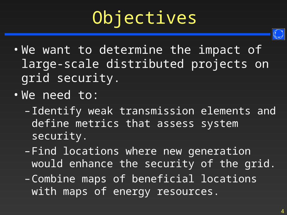
Objectives
• We want to determine the impact of large-scale distributed projects on grid security.
• We need to:– Identify weak transmission elements and
define metrics that assess system security.
– Find locations where new generation would enhance the security of the grid.
– Combine maps of beneficial locations with maps of energy resources.

5
Methodology
• Simulation– Power Flow
– Contingency Analysis
• Security Metrics
• Results– Weak Elements
– Security Indices
– Visualization

6
Power flow Simulation
• Identify weak elements in the system by simulating impacts from lost transmission or capacity (NERC N-1 contingency)
• More importantly, can identify locations in system where new generation can provide grid reliability benefits.

7
Normal Operation Example
100 MW
50 MW
280 MW 187 MW
110 MW 40 Mvar
80 MW 30 Mvar
130 MW 40 Mvar
40 MW 20 Mvar
1.00 pu
1.01 pu
1.04 pu1.04 pu
1.04 pu
0.9930 pu1.05 pu
A
MVA
A
MVA
A
MVA
A
MVA
A
MVA A
MVA
A
MVA
A
MVA
67 MW
67 MW
33 MW 32 MW
57 MW 58 MW
21 MW
21 MW
66 MW 65 MW
11 MW
11 MW
23 MW
42 MW
43 MW 28 MW 29 MW
23 MW
23 MW
150 MW
200 MW 0 Mvar
200 MW 0 Mvar
A
MVA
29 MW 28 MW
OneThree
Four
Two
Five
Six Seven
23 MW
87%
A
MVA
82%
A
MVA
System does not have normal operation thermal violations

8
Contingency Example
100 MW
50 MW
280 MW 188 MW
110 MW 40 Mvar
80 MW 30 Mvar
130 MW 40 Mvar
40 MW 20 Mvar
1.00 pu
1.01 pu
1.04 pu1.04 pu
1.04 pu
0.9675 pu1.05 pu
A
MVA
A
MVA
A
MVA
A
MVAA
MVA
A
MVA 45 MW
45 MW
55 MW 53 MW
0 MW 0 MW
58 MW
56 MW
52 MW 51 MW
26 MW
25 MW
43 MW
36 MW
37 MW 24 MW 25 MW
30 MW
30 MW
150 MW
200 MW 0 Mvar
200 MW 0 Mvar
A
MVA
25 MW 24 MW
OneThree
Four
Two
Five
Six Seven
44 MW
83%
A
MVA
83%
A
MVA
95%
A
MVA
156%
A
MVA
Suppose there is a fault and this line is disconnected
Planning Solutions:New line to bus 3
OR New generation
at bus 3
Then this line getsoverloaded
(is a weak element)This is a serious problem for the
system

9
Contingency Analysis
• Security is determined by the ability of the system to withstand equipment failure.
• Weak elements are those that present overloads in the contingency conditions (congestion).
• Standard approach is to perform a single (N-1) contingency analysis simulation.
• A ranking method will be demonstrated to prioritize transmission planning.

10
Results Organized by Lines, then Contingencies
Sum each value-100 to find the Aggregate Percentage ContingencyOverload (APCO)
Then multiplyby limit to getthe Aggregate MW ContingencyOverload (AMWCO)

11
100 MW
50 MW
280 MW 187 MW
110 MW 40 Mvar
80 MW 30 Mvar
130 MW 40 Mvar
40 MW 20 Mvar
1.00 pu
1.01 pu
1.04 pu1.04 pu
1.04 pu
0.9930 pu1.05 pu
A
MVA
A
MVA
A
MVA
A
MVA
A
MVAA
MVA
A
MVA
A
MVA
67 MW
67 MW
33 MW 32 MW
57 MW 58 MW
21 MW
21 MW
66 MW 65 MW
11 MW
11 MW
23 MW
42 MW
43 MW 28 MW 29 MW
23 MW
23 MW
150 MW
200 MW 0 Mvar
200 MW 0 Mvar
A
MVA
29 MW 28 MW
OneThree
Four
Two
Five
Six Seven
23 MW
87%A
MVA
82%A
MVA
28211470
AMWCO
Weak Element Visualization

12
Determination of Good Locations
Overloaded Linein this direction
New Source
Sink
Transfer helps mitigate the overload by means
of a counter-flow

13
Determination of Good Locations
• Generation could be located to produce counter-flows that mitigate weak element contingency overloads.
• The new injection of power requires decreasing generation somewhere else.– A good assumption is that generation will be
decreased across the system or each control area using participation factors.

14
TLR for Normal Operation
• Need to know how the new generation at a certain bus will impact the flows in a transmission element.
→ Transmission Loading Relief (TLR)
→ Since a TLR is calculated for every bus, the TLR can be used to rank locations that would be beneficial for security.
,ΔMWFlow
TLRΔMWInjection
BRANCHBUS BRANCH
BUS
jki jk
i

15
Specify the weak transmission element
Specify the sink of the transfer
Sensitivities are calculated for each bus

16
TLR for Contingencies
• Need to consider contingencies
• Contingency Transmission Loading Relief (TLR) Sensitivity is the change in the flow of a line due to an injection at a bus assuming a contingency condition.
,, ,
ΔContMWFlowTLR
ΔMWInjectionBRANCH CONT
BUS BRANCH CONT
BUS
jk ci jk c
i

17
Determination of Good Locations
• Equivalent TLR (ETLR):
, ,
Overloaded Contingencies that Elements overloaded branch
,
Contingent Violations
ETLR = TLR
TLR
BUS BUS BRANCH CONT
BUS CONTVIOL
i i jk c
jkjk
i v
v
18
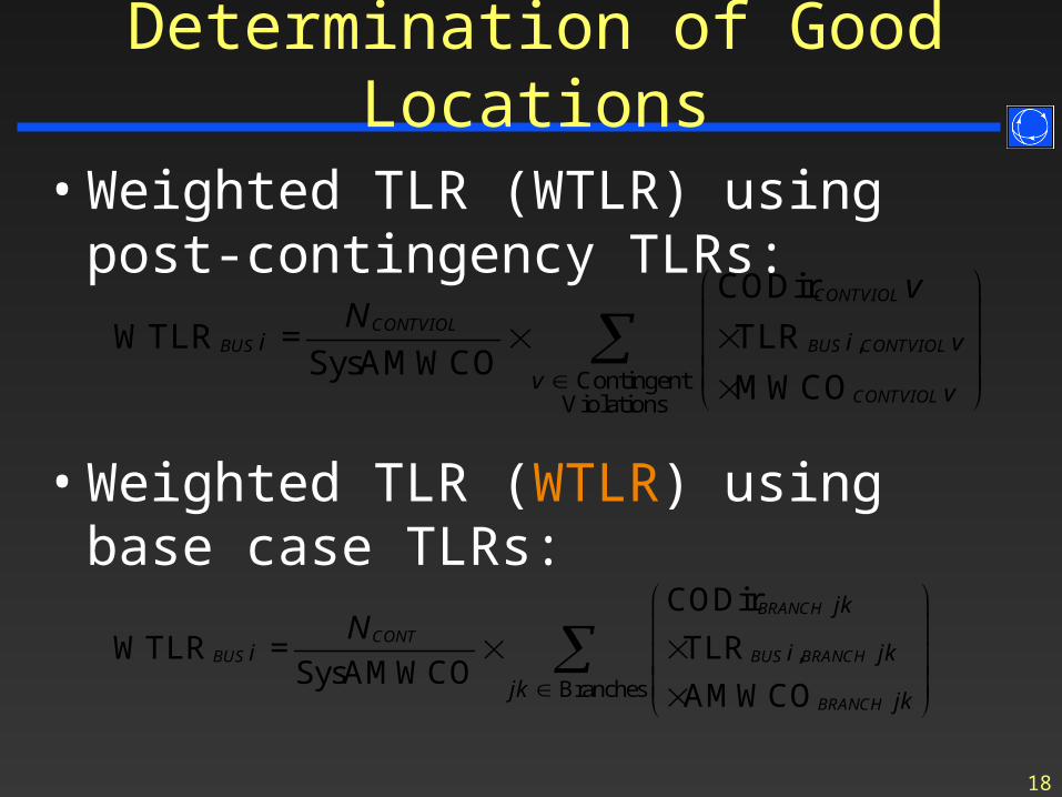
Determination of Good Locations
• Weighted TLR (WTLR) using post-contingency TLRs:
,
Contingent Violations
CODir
WTLR = TLRSysAMWCO
MWCO
CONTVIOL
CONTVIOLBUS BUS CONTVIOL
CONTVIOL
i i v
v v
vN
,
Branches
CODir
WTLR = TLRSysAMWCO
AMWCO
BRANCH
CONTBUS BUS BRANCH
BRANCH
jk
i i jk
jk jk
N
• Weighted TLR (WTLR) using base case TLRs:

19
Weighted TLR (WTLR)
• Complexity: A TLR is computed for each bus, to mitigate a weak element, under a contingency.
• We want a single “weighted” TLR for each bus.
Buses
Weak Elements
Contingencies
Buses
WTLR

20
Calculating WTLRs
• The contingency information (severity and number) of a weak element can be captured by calculating the Aggregate MW Contingency Overload (AMWCO).
• This effectively converts the cube to a table.
Buses
Weak Elements
Buses
Weak Elements
Contingencies

21
Calculating WTLRs
• Need to mitigate the weakest elements first
• Weight the TLR by the weakness of each element, which is given by the AMWCO.
Buses
Weak Elements
Buses
WTLR

22
Meaning of the WTLR
• A WTLR of 0.5 at a bus means that 1MW of new generation injected at the specific bus is likely to reduce 0.5 MW of overload in transmission elements during contingencies.
• Thus, if we inject new generation at high impact buses, re-dispatch the system, and rerun the contingencies, the overloads will decrease.
• Note that the units of the WTLR are:
[MW Contingency Overload]
[MW Installed]
23
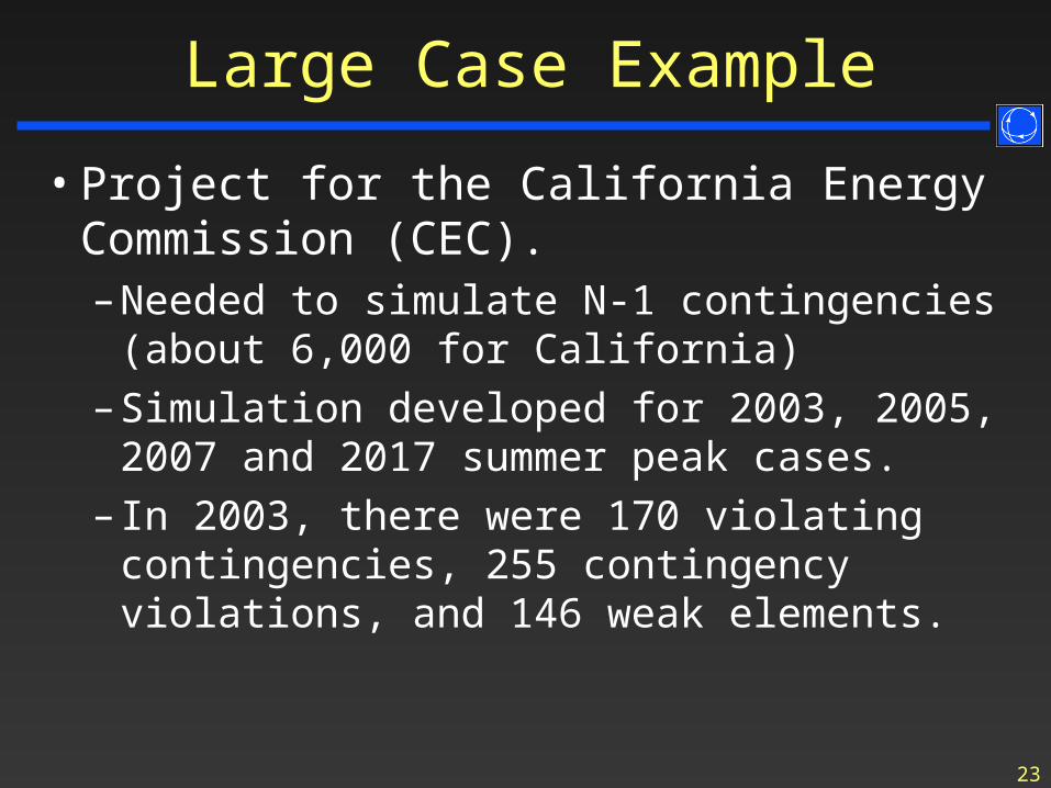
Large Case Example
• Project for the California Energy Commission (CEC).– Needed to simulate N-1 contingencies (about
6,000 for California)
– Simulation developed for 2003, 2005, 2007 and 2017 summer peak cases.
– In 2003, there were 170 violating contingencies, 255 contingency violations, and 146 weak elements.

24
Process Overview
Power Flow Cases
Identify Weak
Elements
Evaluate Locations(WTLR)
GIS Overlay
Test Power Injections at Select
Locations
MARIPO SA
MAD ERA
FRESN O
MERCED
TULARE
KIN GS
MO N TERREY
SAN BEN ITO
SAN TA CLARASAN TA CRUZ
IN YO
MO N O
STAN ISLAUS
PWR 1PWR 1
PWR 1
TO ULUMN E
ALPIN E
CALAVERAS
AMAD O R
EL D O RAD O
SAN MATEO
ALAMED A
MARIN
CO N TRA CO STA
SAN JO AQ UIN
SACRAMEN TO
YO N O
SO LAN O
N APA
SO N O MA
LAKE
MEN D O CH IN O
CO LUSA
SUTTER
BUTTE
GLEN N
PLACER
N EVAD A
SIERRA
YUBA
PLUMAS
TEH AMA
TRIMITY
H UMBO LD TSH ASTA
LASSEN
MO D O C
SISKIYO U
D EL N O RTE
SAN LUIS O BISPO
KERN
SAN TA BARBARA
VEN TURA
LO S AN GELES
SAN BERN ARD IN O
RIVERSID E
IMPERIAL
SAN D IEGO
O RAN GE

25
Result: Weak Element Distribution
0
50
100
150
200
250
300
350
400
0 20 40 60 80 100 120 140 160 180 200 220 240
# Weak Elements
APCO 2003 2005 2007
Both number and weakness of elements increase with time

26
Identification of Weak Elements
2007 2017
The spatial distribution of weak elements seems to follow an identifiable pattern.

27
MARIPOSA
MADERA
FRESNO
MERCED
TULARE
KINGS
MONTERREY
SAN BENITO
SANTA CLARASANTA CRUZ
INYO
MONO
STANISLAUS
PWR 1PWR 1
PWR 1
TOULUMNE
ALPINE
CALAVERAS
AMADOR
EL DORADO
SAN MATEO
ALAMEDA
MARIN
CONTRA COSTA
SAN JOAQUIN
SACRAMENTO
YONO
SOLANO
NAPA
SONOMA
LAKE
MENDOCHINO
COLUSA
SUTTER
BUTTEGLENN
PLACER
NEVADA
SIERRA
YUBA
PLUMAS
TEHAMA
TRIMITY
HUMBOLDTSHASTA
LASSEN
MODOC
SISKIYOU
DEL NORTE
SAN LUIS OBISPO
KERN
SANTA BARBARA
VENTURA
LOS ANGELES
SAN BERNARDINO
RIVERSIDE
IMPERIAL
SAN DIEGO
ORANGE
Good Locations
New generation at green locations will tend to reduce the overloads.
New generation at red-yellow locations will tend to increase the overloads.
Note that higher imports would worsen system security.

28
Local WTLR Visualization
SAN MATEO
ALAMEDA
CONTRA COSTA
CASTROVL
CV BART
HICKS
JEFFERSN
LS PSTAS
MTCALF D
METCALF
METCALF
MTCALF E
MNTA VSA
MONTAVIS
MORAGA
MRAGA 1M
MRAGA 2M
MORAGA
MRAGA 3M
NEWARK F
NEWARK E
NEWARK E
NWK DIST
NEWARK D
NWRK 2 M
NEWARK D
MARTIN C
SANMATEO
SANMATEO
MARTIN C
SARATOGA
TESLA C
TESLA
TESLA E
TESLA JA
TESLA
TESLA JB
TESLA D
UAL COGN
SFIA
MILLBRAE
RAVENSWD
RAVENSWD
DMTAR_SL
SL BART SN LNDRO
JENNY
ALAMEDCT
OAK C115
STATIN L
WHISMAN
MOFT.FLD
LOCKHD 1
LOCKHD 2
S.L.A.C.
MT VIEW
STELLING
JARVIS
CRYOGEN
CYTE PMP
CMP EVRS
FREMNT
CLARMNT
LKWDBART
LKWD_JCT LAKEWD-M
LAKEWD-C
LK_REACT
SERRMNTE
EST PRTL
STATIN D
AMES BS2
AMES BS1 AMES J1B
AMES J1A
AMES DST
WOLFE
E. SHORE
EASTSHRE
EMBRCDRE
EMBRCDRD
LAWRENCE
ROSSTAP1
ROSSMOOR
ROSSTAP2
SANRAMON
TASSAJAR
TRACY
TRACY JC
TRACY
TRCY PMP
STATIN X
DLY CTYP
DALY CTY
GRANT
UCB SUB
UCB JCT1
CLY LNDG
SMATEO3M
STATIN J
ALTM MDW
OAKLND23
MFT.FD J
LCKHD J1
LCKHD J2
SLACTAP1
ADCC
TES JCT
TES SUB
FLOWIND2
JV ENTER
LLNL TAP
LLNLAB
LLNL
WND MSTR
DELTAPMP
VASONA
BELMONT
CLY LNG2
PLO ALTO
LONESTAR
SHREDDER
SHREDJCT
BAIR
JV BART
BAY MDWS
SFIA-MA
SHAWROAD
EST GRND
HNTRS PT
MISSON
LARKIN E
LARKIN F
LARKIN D
POTRERO
BAYSHOR1
BAYSHOR2
AMD JCT
A.M.D
APP MAT
PHLPS_JT
PHILLIPS
BRITTN
PIERCY
IBM-CTLE
IBM-BALY
IBM-HRRS
IBM-HR J
BAILY J3
BAILY J1 BAILY J2
EVRGRN 2
EVRGRN J EVRGRN 1
GILROY
MARKHM J
MARKHAM MARKHMJ2
SWIFT
STONE J
STONE
GEN ELEC
DIXON LD
MABURY
MABURY J
MCKEE
SN JSE A
SJ B E
SJ B F
EDENVALE
EDNVL J3 EDNVL J1
EL PATIO
TRIMBLE
NORTECH
MONTAGUE
ZNKER J1
ZANKER ZNKER J2
KIFER
SCOTT
FMC JCT
FMC
AGNEW
AGNEW J
MILPITAS
waksha j
WAUKESHA
ELLS GTY
KSSN-JC2
HJ HEINZ
TEICHERT
TH.E.DV.
NUMMI
DUMBARTN
MOCCASIN
OAKDLTID
TUOLUMN
CRTEZ
PINEER
HILMAR
MT EDEN
OWENSTAP
OWNBRKWY
CARTWRT
MARITIME
LEPRINO
SAFEWAY
OI GLASS
EBMUDGRY
FIBRJCT2
FIBRJCT1
FIBRBJCT
FIBREBRD
DOMTAR
AEC_TP2
AEC_JCT
SFWY_TP2
AEC_300
AEC_TP1
SFWY_TP1 GWFTRACY
OWENSTP1
OWENSTP2
TCHRTJCT
TCHRT_T2TCHRT_T1
TCY MP1
TCY MP2
TESTAB12
TRAMAX11
LS ESTRS
N_LVMORE
VINEYD_D
VINEYARD
SLACTAP2
EDESTAP1
EDES
EDS GRNT
ELPT_SJ1
ELPT_SJ2
LS ESTRS
NORTHERN
NUMI TAP
NUMI JCT
SANPAULA
UAL TAP
EL ELP11
EVRMTC21
LS NWK11
LS NWK12
LS NWK13
METLS 11
METLS 12
METLS 13
MORSTA11
MORSTA21
MORSTA31
MORSTA41
MTCEVR11
NEWNEW11
SANMAR11
SANMAR12
SANPIT11
SN ELP11
BURLNGME
CAL MEC
DUBLIN
WTLR
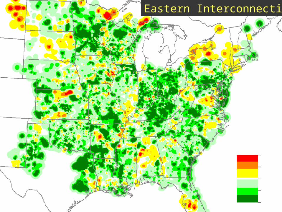
29
1.50
0.75
0.00
–0.75
–1.50
WTLR
Eastern Interconnection

30
Towards a Locational Value
• Determination of locations where new generation would enhance security needs to be combined with availability and economics of energy resources.
• Valuation requires monetizing the security benefits.

31
Towards a Locational Value
• GIS spatial analysis techniques are needed to determine feasible generation alternatives for each location in a large-scale system.
$MW cost of least-cost alternative i ijc g
Based on existing energy potential and technology, a least-cost alternative can be determined for each location.

32
Towards a Locational Value
• Units of WTLR are [AMWCO/MW installed].
• The security cost/benefit can be obtained as follows: – Assume WTLR is negative: Injection reduces the
AMWCO
$, ,MW
cos i i k i k i
benefits k ts k
Value B C s
$$
AMWCO AMWCOMW
i MWi
i
cs
WTLR

33
Security-Penetration Curves
• Once a set of proposed sites is defined, the effect of simultaneous distributed injections with different levels of penetration can be simulated using security-penetration curves.
• The effectiveness of the solution is affected for large injections due to:– Local transfer capability of the grid– Reversed flows

34
Security-Penetration Curves
0
2,000
4,000
6,000
8,000
10,000
12,000
0 650 1300 2000 New Generation
SysAMWCO in 2005
69
500
115
230

35
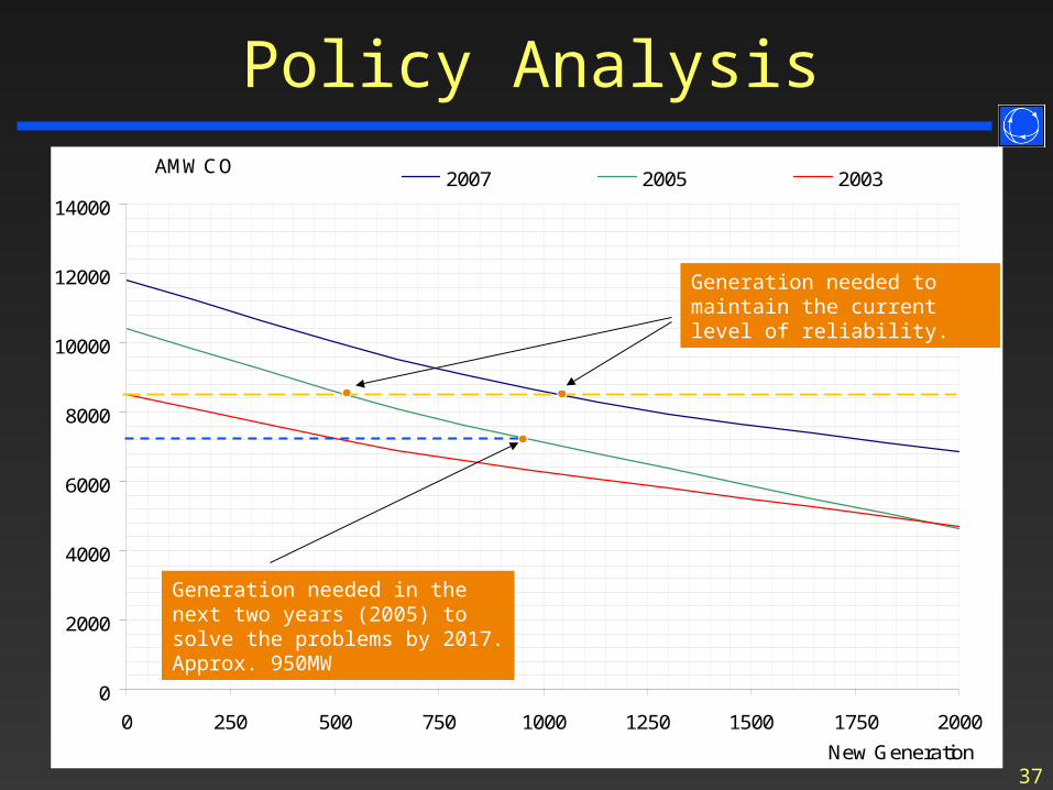
Policy Analysis
• A fundamental goal of integrated electricity systems is to ensure dependable supply to customers.
• This goal cannot be achieved if the system consistently exhibits overloaded elements and congestion.
• System AMWCO can be utilized to:– Evaluate system security for different seasons/years– Design policy goals regarding security
• Can use security-penetration curves

36
Policy Analysis
0
2000
4000
6000
8000
10000
12000
14000
0 250 500 750 1000 1250 1500 1750 2000
New Generation
AMWCO2007 2005 2003
Indicates how much generation is needed to maintain the currentlevel of reliability.Approx. 500MW every two years(at strategic locations)
NewGen
AMWCO
Indicates the effect of new generationApprox. -3.5 MWCO/MW Installed
37
Policy Analysis
0
2000
4000
6000
8000
10000
12000
14000
0 250 500 750 1000 1250 1500 1750 2000
New Generation
AMWCO2007 2005 2003
0
2000
4000
6000
8000
10000
12000
14000
0 250 500 750 1000 1250 1500 1750 2000
New Generation
AMWCO2007 2005 2003
Generation needed to maintain the current level of reliability.
Generation needed in the next two years (2005) to solve the problems by 2017. Approx. 950MW
7300

38
Integrated Model
Power Flow Model
Weak Element Ranking
Spatial Rep. of New Generation
Contingency Analysis
EnergyResources
Maps of Energy Potential
List of Proposed SitesSecurity Indices
Generation Expansion
Security-Penetration
Curves
WTLR Calculation
GIS Spatial Overlay
Transmission Expansion
TransmissionPolicy
Energy Policy