2 Image Formation & Image Sensing - …people.csail.mit.edu/.../RoVis/ch2_image_formation.pdf20...

2

Image Formation & Image Sensing

In this chapter we explore how images are formed and how they are sensedby a computer. Understanding image formation is a prerequisite for fullunderstanding of the methods for recovering information from images. Inanalyzing the process by which a three-dimensional world is projected ontoa two-dimensional image plane, we uncover the two key questions of imageformation:

• What determines where the image of some point will appear?

• What determines how bright the image of some surface will be?

The answers to these two questions require knowledge of image projectionand image radiometry, topics that will be discussed in the context of simplelens systems.

A crucial notion in the study of image formation is that we live in avery special visual world. It has particular features that make it possi-ble to recover information about the three-dimensional world from one ormore two-dimensional images. We discuss this issue and point out imag-ing situations where these special constraint do not apply, and where it isconsequently much harder to extract information from images.

We also study the basic mechanism of typical image sensors, and howinformation in different spectral bands may be obtained and processed.

2.1 Two Aspects of Image Formation 19

Following a brief discussion of color, the chapter closes with a discussion ofnoise and reviews some concepts from the fields of probability and statis-tics. This is a convenient point to introduce convolution in one dimension,an idea that will be exploited later in its two-dimensional generalization.Readers familiar with these concepts may omit these sections without lossof continuity. The chapter concludes with a discussion of the need forquantization of brightness measurements and for tessellations of the imageplane.

2.1 Two Aspects of Image Formation

Before we can analyze an image, we must know how it is formed. An imageis a two-dimensional pattern of brightness. How this pattern is producedin an optical image-forming system is best studied in two parts: first, weneed to find the geometric correspondence between points in the scene andpoints in the image; then we must figure out what determines the brightnessat a particular point in the image.

2.1.1 Perspective Projection

Consider an ideal pinhole at a fixed distance in front of an image plane(figure 2-1). Assume that an enclosure is provided so that only light comingthrough the pinhole can reach the image plane. Since light travels alongstraight lines, each point in the image corresponds to a particular directiondefined by a ray from that point through the pinhole. Thus we have thefamiliar perspective projection.

We define the optical axis, in this simple case, to be the perpendic-ular from the pinhole to the image plane. Now we can introduce a con-venient Cartesian coordinate system with the origin at the pinhole andz-axis aligned with the optical axis and pointing toward the image. Withthis choice of orientation, the z components of the coordinates of pointsin front of the camera are negative. We use this convention, despite thedrawback, because it gives us a convenient right-hand coordinate system(with the x-axis to the right and the y-axis upward).

We would like to compute where the image P ′ of the point P on someobject in front of the camera will appear (figure 2-1). We assume that noother object lies on the ray from P to the pinhole O. Let r = (x, y, z)T bethe vector connecting O to P , and r′ = (x′, y′, f ′)T be the vector connectingO to P ′. (As explained in the appendix, vectors will be denoted by boldfaceletters. We commonly deal with column vectors, and so must take the

20 Image Formation & Image Sensing

transpose, indicated by the superscript T , when we want to write them interms of the equivalent row vectors.)

Here f ′ is the distance of the image plane from the pinhole, while x′

and y′ are the coordinates of the point P ′ in the image plane. The twovectors r and r′ are collinear and differ only by a (negative) scale factor.If the ray connecting P to P ′ makes an angle α with the optical axis, thenthe length of r is just

r = −z sec α = −(r · z) sec α,

where z is the unit vector along the optical axis. (Remember that z isnegative for a point in front of the camera.)

The length of r′ is

r′ = f ′ sec α,

and so

1f ′ r

′ =1

r · z r.

2.1 Two Aspects of Image Formation 21

In component form this can be written as

x′

f ′ =x

zand

y′

f ′ =y

z.

Sometimes image coordinates are normalized by dividing x′ and y′ by f ′

in order to simplify the projection equations.

2.1.2 Orthographic Projection

Suppose we form the image of a plane that lies parallel to the image atz = z0. Then we can define m, the (lateral) magnification, as the ratioof the distance between two points measured in the image to the distancebetween the corresponding points on the plane. Consider a small interval(δx, δy, 0)T on the plane and the corresponding small interval (δx′, δy′, 0)T

in the image. Then

m =

√(δx′)2 + (δy′)2√(δx)2 + (δy)2

=f ′

−z0,

where −z0 is the distance of the plane from the pinhole. The magnificationis the same for all points in the plane. (Note that m < 1, except in thecase of microscopic imaging.)

A small object at an average distance −z0 will give rise to an image thatis magnified by m, provided that the variation in z over its visible surfaceis not significant compared to −z0. The area occupied by the image ofan object is proportional to m2. Objects at different distances from theimaging system will, of course, be imaged with different magnifications.Let the depth range of a scene be the range of distances of surfaces fromthe camera. The magnification is approximately constant when the depthrange of the scene being imaged is small relative to the average distance ofthe surfaces from the camera. In this case we can simplify the projectionequations to read

x′ = −mx and y′ = −my,

where m = f ′/(−z0) and −z0 is the average value of −z. Often the scalingfactor m is set to 1 or −1 for convenience. Then we can further simplifythe equations to become

x′ = x and y′ = y.

This orthographic projection (figure 2-2), can be modeled by rays parallelto the optical axis (rather than ones passing through the origin). The


difference between perspective and orthographic projection is small whenthe distance to the scene is much larger than the variation in distanceamong objects in the scene.

The field of view of an imaging system is the angle of the cone ofdirections encompassed by the scene that is being imaged. This cone ofdirections clearly has the same shape and size as the cone obtained byconnecting the edge of the image plane to the center of projection. A“normal” lens has a field of view of perhaps 25◦ by 40◦. A telephoto lensis one that has a long focal length relative to the image size and thus anarrow field of view. Conversely, a wide-angle lens has a short focal lengthrelative to the image size and thus a wide field of view. A rough rule ofthumb is that perspective effects are significant when a wide-angle lens isused, while images obtained using a telephoto lenses tend to approximateorthographic projection. We shall show in exercise 2-11 that this rule isnot exact.

2.2 Brightness 23


2.2 Brightness

The more difficult, and more interesting, question of image formation iswhat determines the brightness at a particular point in the image. Bright-ness is an informal term used to refer to at least two different concepts:image brightness and scene brightness. In the image, brightness is relatedto energy flux incident on the image plane and can be measured in a num-ber of ways. Here we introduce the term irradiance to replace the informalterm image brightness. Irradiance is the power per unit area (W·m−2—watts per square meter) of radiant energy falling on a surface (figure 2-3a).In the figure, E denotes the irradiance, while δP is the power of the radiantenergy falling on the infinitesimal surface patch of area δA. The blackeningof a film in a camera, for example, is a function of the irradiance. (As weshall discuss a little later, the measurement of brightness in the image alsodepends on the spectral sensitivity of the sensor.) The irradiance at a par-ticular point in the image will depend on how much light arrives from thecorresponding object point (the point found by following the ray from the

2.2 Brightness 25

image point through the pinhole until it meets the surface of an object).

2.3 Lenses 27

In the scene, brightness is related to the energy flux emitted from asurface. Different points on the objects in front of the imaging system willhave different brightnesses, depending on how they are illuminated andhow they reflect light. We now introduce the term radiance to substitutefor the informal term scene brightness. Radiance is the power per unitforeshortened area emitted into a unit solid angle (W·m−2·sr−1—watts persquare meter per steradian) by a surface (figure 2-3b). In the figure, L is theradiance and δ2P is the power emitted by the infinitesimal surface patchof area δA into an infinitesimal solid angle δω. The apparent complexityof the definition of radiance stems from the fact that a surface emits lightinto a hemisphere of possible directions, and we obtain a finite amountonly by considering a finite solid angle of these directions. In general theradiance will vary with the direction from which the object is viewed. Weshall discuss radiometry in detail later, when we introduce the reflectancemap.

We are interested in the radiance of surface patches on objects becausewhat we measure, image irradiance, turns out to be proportional to sceneradiance, as we show later. The constant of proportionality depends on theoptical system. To gather a finite amount of light in the image plane wemust have an aperture of finite size. The pinhole, introduced in the lastsection, must have a nonzero diameter. Our simple analysis of projectionno longer applies, though, since a point in the environment is now imagedas a small circle. This can be seen by considering the cone of rays passingthrough the circular pinhole with its apex at the object point.

We cannot make the pinhole very small for another reason. Becauseof the wave nature of light, diffraction occurs at the edge of the pinholeand the light is spread over the image. As the pinhole is made smaller andsmaller, a larger and larger fraction of the incoming light is deflected farfrom the direction of the incoming ray.

2.3 Lenses

In order to avoid the problems associated with pinhole cameras, we nowconsider the use of a lens in an image-forming system. An ideal lens pro-duces the same projection as the pinhole, but also gathers a finite amountof light (figure 2-4). The larger the lens, the larger the solid angle it sub-tends when seen from the object. Correspondingly it intercepts more ofthe light reflected from (or emitted by) the object. The ray through the


center of the lens is undeflected. In a well-focused system the other rays

2.3 Lenses 29

are deflected to reach the same image point as the central ray.

2.3 Lenses 31

An ideal lens has the disadvantage that it only brings to focus lightfrom points at a distance −z given by the familiar lens equation

1z′ +

1−z

=1f

,

where z′ is the distance of the image plane from the lens and f is the focallength (figure 2-4). Points at other distances are imaged as little circles.This can be seen by considering the cone of light rays passing through thelens with apex at the point where they are correctly focused. The size ofthe blur circle can be determined as follows: A point at distance −z isimaged at a point z′ from the lens, where

1z′ +

1−z

=1f

,

and so

(z′ − z′) =f

(z + f)f

(z + f)(z − z).

If the image plane is situated to receive correctly focused images of objectsat distance −z, then points at distance −z will give rise to blur circles ofdiameter

d

z′ |z′ − z′| ,

where d is the diameter of the lens. The depth of field is the range ofdistances over which objects are focused “sufficiently well,” in the sensethat the diameter of the blur circle is less than the resolution of the imagingdevice. The depth of field depends, of course, on what sensor is used, butin any case it is clear that the larger the lens aperture, the less the depthof field. Clearly also, errors in focusing become more serious when a largeaperture is employed.

Simple ray-tracing rules can help in understanding simple lens combi-nations. As already mentioned, the ray through the center of the lens isundeflected. Rays entering the lens parallel to the optical axis converge toa point on the optical axis at a distance equal to the focal length. This fol-lows from the definition of focal length as the distance from the lens wherethe image of an object that is infinitely far away is focused. Conversely,rays emitted from a point on the optical axis at a distance equal to the focallength from the lens are deflected to emerge parallel to the optical axis onthe other side of the lens. This follows from the reversibility of rays. At aninterface between media of different refractive indices, the same reflectionand refraction angles apply to light rays traveling in opposite directions.


A simple lens is made by grinding and polishing a glass blank so thatits two surfaces have shapes that are spherical. The optical axis is the linethrough the centers of the two spheres. Any such simple lens will havea number of defects or aberrations. For this reason one usually combinesseveral simple lenses, carefully lining up their individual optical axes, so asto make a compound lens with better properties.

A useful model of such a system of lenses is the thick lens (figure 2-5).One can define two principal planes perpendicular to the optical axis, andtwo nodal points where these planes intersect the optical axis. A ray arriv-ing at the front nodal point leaves the rear nodal point without changingdirection. This defines the projection performed by the lens. The distancebetween the two nodal points is the thickness of the lens. A thin lens is

2.3 Lenses 33

one in which the two nodal points can be considered coincident.

2.3 Lenses 35

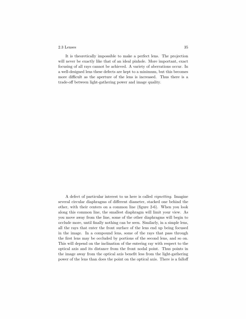
It is theoretically impossible to make a perfect lens. The projectionwill never be exactly like that of an ideal pinhole. More important, exactfocusing of all rays cannot be achieved. A variety of aberrations occur. Ina well-designed lens these defects are kept to a minimum, but this becomesmore difficult as the aperture of the lens is increased. Thus there is atrade-off between light-gathering power and image quality.

A defect of particular interest to us here is called vignetting. Imagineseveral circular diaphragms of different diameter, stacked one behind theother, with their centers on a common line (figure 2-6). When you lookalong this common line, the smallest diaphragm will limit your view. Asyou move away from the line, some of the other diaphragms will begin toocclude more, until finally nothing can be seen. Similarly, in a simple lens,all the rays that enter the front surface of the lens end up being focusedin the image. In a compound lens, some of the rays that pass throughthe first lens may be occluded by portions of the second lens, and so on.This will depend on the inclination of the entering ray with respect to theoptical axis and its distance from the front nodal point. Thus points inthe image away from the optical axis benefit less from the light-gatheringpower of the lens than does the point on the optical axis. There is a falloff


in sensitivity with distance from the center of the image.

2.3 Lenses 37


Another important consideration is that the aberrations of a lens in-crease in magnitude as a power of the angle between the incident ray andthe optical axis. Aberrations are classified by their order, that is, the powerof the angle that occurs in this relationship. Points on the optical axis maybe quite well focused, while those in a corner of the image are smeared out.For this reason, only a limited portion of the image plane is usable. Themagnitude of an aberration defect also increases as a power of the distancefrom the optical axis at which a ray passes through the lens. Thus theimage quality can be improved by using only the central portion of a lens.

One reason for introducing diaphragms into a lens system is to im-prove image quality in a situation where it is not necessary to utilize fullythe light-gathering power of the system. As already mentioned, fixed di-aphragms ensure that rays entering at a large angle to the optical axis donot pass through the outer regions of any of the lenses. This improvesimage quality in the outer regions of the image, but at the same timegreatly increases vignetting. In most common uses of lenses this is notan important matter, since people are astonishingly insensitive to smoothspatial variations in image brightness. It does matter in machine vision,however, since we use the measurements of image brightness (irradiance)to determine the scene brightness (radiance).

2.4 Our Visual World

How can we hope to recover information about the three-dimensional worldusing a mere two-dimensional image? It may seem that the available in-formation is not adequate, even if we take several images. Yet biologicalsystems interact intelligently with the environment using visual informa-tion. The puzzle is solved when we consider the special nature of our usualvisual world. We are immersed in a homogeneous transparent medium, andthe objects we look at are typically opaque. Light rays are not refractedor absorbed in the environment, and we can follow a ray from an imagepoint through the lens until it reaches some surface. The brightness ata point in the image depends only on the brightness of the correspondingsurface patch. Surfaces are two-dimensional manifolds, and their shape canbe represented by giving the distance z(x′, y′) to the surface as a functionof the image coordinates x′ and y′.

This is to be contrasted with a situation in which we are looking intoa volume occupied by a light-absorbing material of varying density. Herewe may specify the density ρ(x, y, z) of the material as a function of thecoordinates x, y, and z. One or more images provide enough constraint to

2.4 Our Visual World 39

recover information about a surface, but not about a volume. In theory,an infinite number of images is needed to solve the problem of tomography,that is, to determine the density of the absorbing material.

Conditions of homogeneity and transparency may not always hold ex-actly. Distant mountains appear changed in color and contrast, while indeserts we may see mirages. Image analysis based on the assumption thatconditions are as stated may go awry when the assumptions are violated,and so we can expect that both biological and machine vision systems willbe misled in such situations. Indeed, some optical illusions can be ex-plained in this way. This does not mean that we should abandon theseadditional constraints, for without them the solution of the problem of re-covering information about the three-dimensional world from images wouldbe ambiguous.

Our usual visual world is special indeed. Imagine being immersedinstead in a world with varying concentrations of pigments dispersed withina gelatinous substance. It would not be possible to recover the distributionsof these absorbing substances in three dimensions from one view. Therejust would not be enough information. Analogously, single X-ray imagesare not useful unless there happens to be sharp contrast between differentmaterials, like bone and tissue. Otherwise a very large number of viewsmust be taken and a tomographic reconstruction attempted. It is perhapsa good thing that we do not possess Superman’s X-ray vision capabilities!

By and large, we shall confine our attention to images formed by con-ventional optical means. We shall avoid high-magnification microscopicimages, for instance, where many substances are effectively transparent,or at least translucent. Similarly, images on a very large scale often showthe effects of absorption and refraction in the atmosphere. Interestingly,other modalities do sometimes provide us with images much like the oneswe are used to. Examples include scanning electron microscopes (SEM)and synthetic-aperture radar systems (SAR), both of which produce im-ages that are easy to interpret. So there is some hope of analyzing themusing the methods discussed here.

In view of the importance of surfaces, we might hope that a machinevision system could be designed to recover the shapes of surfaces given oneor more images. Indeed, there has been some success in this endeavor, aswe shall see in chapter 10, where we discuss the recovery of shape fromshading. Detailed understanding of the imaging process allows us to re-cover quantitative information from images. The computed shape of asurface may be used in recognition, inspection, or in planning the path of


a mechanical manipulator.

2.5 Image Sensing

Almost all image sensors depend on the generation of electron–hole pairswhen photons strike a suitable material. This is the basic process in bi-ological vision as well as photography. Image sensors differ in how theymeasure the flux of charged particles. Some devices use an electric fieldin a vacuum to separate the electrons from the surface where they are lib-erated (figure 2-7a). In other devices the electrons are swept through a

2.5 Image Sensing 41

depleted zone in a semiconductor (figure 2-7b).


Not all incident photons generate an electron–hole pair. Some passright through the sensing layer, some are reflected, and others lose energyin different ways. Further, not all electrons find their way into the detect-ing circuit. The ratio of the electron flux to the incident photon flux iscalled the quantum efficiency, denoted q(λ). The quantum efficiency de-pends on the energy of the incident photon and hence on its wavelength λ.It also depends on the material and the method used to collect the liber-ated electrons. Older vacuum devices tend to have coatings with relativelylow quantum efficiency, while solid-state devices are near ideal for somewavelengths. Photographic film tends to have poor quantum efficiency.

2.5.1 Sensing Color

The sensitivity of a device varies with the wavelength of the incident light.Photons with little energy tend to go right through the material, whilevery energetic photons may be stopped before they reach the sensitivelayer. Each material has its characteristic variation of quantum efficiencywith wavelength.

For a small wavelength interval δλ, let the flux of photons with energyequal to or greater than λ, but less than λ + δλ, be b(λ) δλ. Then thenumber of electrons liberated is∫ ∞

−∞b(λ)q(λ) dλ.

If we use sensors with different photosensitive materials, we obtain differentimages because their spectral sensitivities are different. This can be helpfulin distinguishing surfaces that have similar gray-levels when imaged withone sensor, yet give rise to different gray-levels when imaged with a differ-ent sensor. Another way to achieve this effect is to use the same sensingmaterial but place filters in front of the camera that selectively absorb dif-ferent parts of the spectrum. If the transmission of the ith filter is fi(λ),the effective quantum efficiency of the combination of that filter and thesensor is fi(λ)q(λ).

How many different filters should we use? The ability to distinguishamong materials grows as more images are taken through more filters.The measurements are correlated, however, because most surfaces have asmooth variation of reflectance with wavelength. Typically, little is gainedby using very many filters.

The human visual system uses three types of sensors, called cones, indaylight conditions. Each of these cone types has a particular spectral


sensitivity, one of them peaking in the long wavelength range, one in themiddle, and one in the short wavelength range of the visible spectrum,which extends from about 400 nm to about 700 nm. There is considerableoverlap between the sensitivity curves. Machine vision systems often alsouse three images obtained through red, green, and blue filters. It shouldbe pointed out, however, that the results have little to do with humancolor sensations unless the spectral response curves happen to be linearcombinations of the human spectral response curves, as discussed below.

One property of a sensing system with a small number of sensor typeshaving different spectral sensitivities is that many different spectral distri-butions will produce the same output. The reason is that we do not measurethe spectral distributions themselves, but integrals of their product withthe spectral sensitivity of particular sensor types. The same applies to bio-logical systems, of course. Colors that appear indistinguishable to a humanobserver are said to be metameric. Useful information about the spectralsensitivities of the human visual system can be gained by systematicallyexploring metamers. The results of a large number of color-matching ex-periments performed by many observers have been averaged and used tocalculate the so-called tristimulus or standard observer curves. These havebeen published by the Commission Internationale de l’Eclairage (CIE) andare shown in figure 2-8. A given spectral distribution is evaluated as fol-lows: The spectral distribution is multiplied in turn by each of the threefunctions x(λ), y(λ), and z(λ). The products are integrated over the visiblewavelength range. The three results X, Y , and Z are called the tristimulusvalues. Two spectral distributions that result in the same values for thesethree quantities appear indistinguishable when placed side by side undercontrolled conditions. (By the way, the spectral distributions used here areexpressed in terms of energy per unit wavelength interval, not photon flux.)

The actual spectral response curves of the three types of cones cannotbe determined in this way, however. There is some remaining ambiguity.It is known that the tristimulus curves are fixed linear transforms of thesespectral response curves. The coefficients of the transformation are notknown accurately.

We show in exercise 2-14 that a machine vision system with the samecolor-matching properties as the human color vision system must have sen-sitivities that are linear transforms of the human cone response curves. Thisin turn implies that the sensitivities must be linear transforms of the knownstandard observer curves. Unfortunately, this rule has rarely been observedwhen color-sensing systems were designed in the past. (Note that we are


not addressing the problem of color sensations; we are only interested in


having the machine confuse the same colors as the standard observer.)


2.5.2 Randomness and Noise

It is difficult to make accurate measurements of image brightness. In thissection we discuss the corrupting influence of noise on image sensing. Inorder to do this, we need to discuss random variables and the probabilitydensity distribution. We shall also take the opportunity to introduce theconcept of convolution in the one-dimensional case. Later, we shall en-counter convolution again, applied to two-dimensional images. The readerfamiliar with these concepts may want to skip this section.

Measurements are affected by fluctuations in the signal being mea-sured. If the measurement is repeated, somewhat differing results may beobtained. Typically, measurements will cluster around the “correct” value.We can talk of the probability that a measurement will fall within a certaininterval. Roughly speaking, this is the limit of the ratio of the number ofmeasurements that fall in that interval to the total number of trials, as thetotal number of trials tends to infinity. (This definition is not quite ac-curate, since any particular sequence of experiments may produce resultsthat do not tend to the expected limit. It is unlikely that they are far off,however. Indeed, the probability of the limit tending to an answer that is


not the desired one is zero.)


Now we can define the probability density distribution, denoted p(x).The probability that a random variable will be equal to or greater thanx, but less than x + δx, tends to p(x)δx as δx tends to zero. (Thereis a subtle problem here, since for a given number of trials the numberfalling in the interval will tend to zero as the size of the interval tendsto zero. This problem can be sidestepped by considering the cumulativeprobability distribution, introduced below.) A probability distribution canbe estimated from a histogram obtained from a finite number of trials(figure 2-9). From our definition follow two important properties of anyprobability distribution p(x):

p(x) ≥ 0 for all x, and∫ ∞

−∞p(x) dx = 1.

Often the probability distribution has a strong peak near the “correct,” or“expected,” value. We may define the mean accordingly as the center ofarea, µ, of this peak, defined by the equation

µ

∫ ∞

−∞p(x) dx =

∫ ∞

−∞x p(x) dx.

Since the integral of p(x) from minus infinity to plus infinity is one,

µ =∫ ∞

−∞x p(x) dx.

The integral on the right is called the first moment of p(x).Next, to estimate the spread of the peak of p(x), we can take the second

moment about the mean, called the variance:

σ2 =∫ ∞

−∞(x − µ)2 p(x) dx.

The square root of the variance, called the standard deviation, is a usefulmeasure of the width of the distribution.

Another useful concept is the cumulative probability distribution,

P (x) =∫ x

−∞p(t) dt,

which tells us the probability that the random variable will be less thanor equal to x. The probability density distribution is just the derivative ofthe cumulative probability distribution. Note that

limx→∞ P (x) = 1.


One way to improve accuracy is to average several measurements, assumingthat the “noise” in them will be independent and tend to cancel out. Tounderstand how this works, we need to be able to compute the probability


distribution of a sum of several random variables.


Suppose that x is a sum of two independent random variables x1 andx2 and that p1(x1) and p2(x2) are their probability distributions. How dowe find p(x), the probability distribution of x = x1 + x2? Given x2, weknow that x1 must lie between x − x2 and x + δx − x2 in order for x to liebetween x and x + δx (figure 2-10). The probability that this will happenis p1(x−x2) δx. Now x2 can take on a range of values, and the probabilitythat it lies in a particular interval x2 to x2 + δx2 is just p2(x2) δx2. Tofind the probability that x lies between x and x+ δx we must integrate theproduct over all x2. Thus

p(x) δx =∫ ∞

−∞p1(x − x2) δx p2(x2) dx2,

or

p(x) =∫ ∞

−∞p1(x − t) p2(t) dt.

By a similar argument one can show that

p(x) =∫ ∞

−∞p2(x − t) p1(t) dt,

in which the roles of x1 and x2 are reversed. These correspond to two waysof integrating the product of the probabilities over the narrow diagonal strip(figure 2-10). In either case, we talk of a convolution of the distributionsp1 and p2, written as

p = p1 ⊗ p2.

We have just shown that convolution is commutative.We show in exercise 2-16 that the mean of the sum of several random

variables is equal to the sum of the means, and that the variance of thesum equals the sum of the variances. Thus if we compute the average ofN independent measurements,

x =1N

N∑i=1

xi,

each of which has mean µ and standard deviation σ, the mean of the resultis also µ, while the standard deviation is σ/

√N since the variance of the

sum is Nσ2. Thus we obtain a more accurate result, that is, one lessaffected by “noise.” The relative accuracy only improves with the squareroot of the number of measurements, however.


A probability distribution that is of great practical interest is the nor-mal or Gaussian distribution

p(x) =1√2πσ

e− 12 ( x−µ

σ )2

with mean µ and standard deviation σ. The noise in many measurementprocesses can be modeled well using this distribution.

So far we have been dealing with random variables that can take onvalues in a continuous range. Analogous methods apply when the possiblevalues are in a discrete set. Consider the electrons liberated during a fixedinterval by photons falling on a suitable material. Each such event is inde-pendent of the others. It can be shown that the probability that exactly n

are liberated in a time interval T is

Pn = e−m mn

n!

for some m. This is the Poisson distribution. We can calculate the averagenumber liberated in time T as follows:

∞∑n=1

ne−m mn

n!= me−m

∞∑n=1

mn−1

(n − 1)!.

But∞∑

n=1

mn−1

(n − 1)!=

∞∑n=0

mn

n!= em,

so the average is just m. We show in exercise 2-18 that the variance is alsom. The standard deviation is thus

√m, so that the ratio of the standard

deviation to the mean is 1/√

m. The measurement becomes more accuratethe longer we wait, since more electrons are gathered. Again, the ratio ofthe “signal” to the “noise” only improves as the square root of the averagenumber of electrons collected, however.

To obtain reasonable results, many electrons must be measured. It canbe shown that a Poisson distribution with mean m is almost the same asa Gaussian distribution with mean m and variance m, provided that m islarge. The Gaussian distribution is often easier to work with. In any case,to obtain a standard deviation that is one-thousandth of the mean, onemust wait long enough to collect a million electrons. This is a small chargestill, since one electron carries only

e = 1.602192 . . . × 10−19 Coulomb.


Even a million electrons have a charge of only about 160 fC (femto-Coulomb). (The prefix femto- denotes a multiplier of 10−15.) It is noteasy to measure such a small charge, since noise is introduced in the mea-surement process.

The number of electrons liberated from an area δA in time δt is

N = δA δt

∫ ∞

−∞b(λ) q(λ) dλ,

where q(λ) is the quantum efficiency and b(λ) is the image irradiance inphotons per unit area. To obtain a usable result, then, electrons must becollected from a finite image area over a finite amount of time. There isthus a trade-off between (spatial and temporal) resolution and accuracy.

A measurement of the number of electrons liberated in a small areaduring a fixed time interval produces a result that is proportional to theirradiance (for fixed spectral distribution of incident photons). These mea-surements are quantized in order to read them into a digital computer.This is done by analog-to-digital (A/D) conversion. The result is called agray-level. Since it is difficult to measure irradiance with great accuracy,it is reasonable to use a small set of numbers to represent the irradiancelevels. The range 0 to 255 is often employed—requiring just 8 bits pergray-level.

2.5.3 Quantization of the Image

Because we can only transmit a finite number of measurements to a com-puter, spatial quantization is also required. It is common to make mea-surements at the nodes of a square raster or grid of points. The image isthen represented as a rectangular array of integers. To obtain a reason-able amount of detail we need many measurements. Television frames, forexample, might be quantized into 450 lines of 560 picture cells, sometimesreferred to as pixels.

Each number represents the average irradiance over a small area. Wecannot obtain a measurement at a point, as discussed above, because theflux of light is proportional to the sensing area. At first this might appearas a shortcoming, but it turns out to be an advantage. The reason is thatwe are trying to use a discrete set of numbers to represent a continuousdistribution of brightness, and the sampling theorem tells us that this canbe done successfully only if the continuous distribution is smooth, thatis, if it does not contain high-frequency components. One way to make a


smooth distribution of brightness is to look at the image through a filterthat averages over small areas.

What is the optimal size of the sampling areas? It turns out thatreasonable results are obtained if the dimensions of the sampling areas areapproximately equal to their spacing. This is fortunate because it allows usto pack the image plane efficiently with sensing elements. Thus no photonsneed be wasted, nor must adjacent sampling areas overlap.

We have some latitude in dividing up the image plane into sensingareas. So far we have been discussing square areas on a square grid. Thepicture cells could equally well be rectangular, resulting in a different res-olution in the horizontal and vertical directions. Other arrangements arealso possible. Suppose we want to tile the plane with regular polygons. Thetiles should not overlap, yet together they should cover the whole plane.We shall show in exercise 2-21 that there are exactly three tessellations,


based on triangles, squares, and hexagons (figure 2-11).

2.6 References 61

It is easy to see how a square sampling pattern is obtained simply bytaking measurements at equal intervals along equally spaced lines in theimage. Hexagonal sampling is almost as easy, if odd-numbered lines areoffset by half a sampling interval from even-numbered lines. In televisionscanning, the odd-numbered lines are read out after all the even-numberedlines because of field interlace, and so this scheme is particularly easy toimplement. Hexagons on a triangular grid have certain advantages, whichwe shall come to later.

2.6 References

There are many standard references on basic optics, including Principles ofOptics: Electromagnetic Theory of Propagation, Interference and Diffrac-tion of Light by Born & Wolf [1975], Handbook of Optics, edited by Driscoll& Vaughan [1978], Applied Optics: A Guide to Optical System Design byLevi [volume 1, 1968; volume 2, 1980], and the classic Optics by Sears[1949]. Lens design and aberrations are covered by Kingslake in Lens De-sign Fundamentals [1978]. Norton discusses the basic workings of a largevariety of sensors in Sensor and Analyzer Handbook [1982]. Barbe editedCharge-Coupled Devices [1980], a book that includes some information onthe use of CCDs in image sensors.

There is no shortage of books on probability and statistics. One suchis Drake’s Fundamentals of Applied Probability Theory [1967].

Color vision is not treated in detail here, but is mentioned again inchapter 9 where we discuss the recovery of lightness. For a general discus-sion of color matching and tristimulus values see the first few chapters ofColor in Business, Science, and Industry by Judd & Wyszeck [1975].

Some issues of color reproduction, including what constitutes an ap-propriate sensor system, are discussed by Horn [1984a]. Further referenceson color vision may be found at the end of chapter 9.

Straight lines in the three-dimensional world are projected as straightlines into the two-dimensional image. The projections of parallel lines inter-sect in a vanishing point. This is the point where a line parallel to the givenlines passing through the center of projection intersects the image plane.In the case of rectangular objects, a great deal of information can be re-covered from lines in the images and their intersections. See, for example,Barnard [1983].

When the medium between us and the scene being imaged is not per-fectly transparent, the interpretation of images becomes more complicated.See, for example, Sjoberg & Horn [1983]. The reconstruction of absorbing


density in a volume from measured ray attenuation is the subject of to-mography; a book on this subject has been edited by Herman [1979].

2.7 Exercises

2-1 What is the shape of the image of a sphere? What is the shape of theimage of a circular disk? Assume perspective projection and allow the disk to liein a plane that can be tilted with respect to the image plane.

2-2 Show that the image of an ellipse in a plane, not necessarily one parallel tothe image plane, is also an ellipse. Show that the image of a line in space is a linein the image. Assume perspective projection. Describe the brightness patternsin the image of a polyhedral object with uniform surface properties.

2-3 Suppose that an image is created by a camera in a certain world. Nowimagine the same camera placed in a similar world in which everything is twiceas large and all distances between objects have also doubled. Compare the newimage with the one formed in the original world. Assume perspective projection.

2-4 Suppose that an image is created by a camera in a certain world. Nowimagine the same camera placed in a similar world in which everything has halfthe reflectance and the incident light has been doubled. Compare the new imagewith the one formed in the original world. Hint: Ignore interflections, that is,illumination of one part of the scene by light reflected from another.

2-5 Show that in a properly focused imaging system the distance f ′ from thelens to the image plane equals (1+m)f , where f is the focal length and m is themagnification. This distance is called the effective focal length. Show that thedistance between the image plane and an object must be(

m + 2 +1m

)f.

How far must the object be from the lens for unit magnification?

2-6 What is the focal length of a compound lens obtained by placing two thinlenses of focal length f1 and f2 against one another? Hint: Explain why an objectat a distance f1 on one side of the compound lens will be focused at a distancef2 on the other side.

2-7 The f-number of a lens is the ratio of the focal length to the diameter ofthe lens. The f-number of a given lens (of fixed focal length) can be increasedby introducing an aperture that intercepts some of the light and thus in effectreduces the diameter of the lens. Show that image brightness will be inverselyproportional to the square of the f-number. Hint: Consider how much light isintercepted by the aperture.

2.7 Exercises 63

2-8 When a camera is used to obtain metric information about the world, itis important to have accurate knowledge of the parameters of the lens, includingthe focal length and the positions of the principal planes. Suppose that a patternin a plane at distance x on one side of the lens is found to be focused best on aplane at a distance y on the other side of the lens (figure 2-12). The distancesx and y are measured from an arbitrary but fixed point in the lens. How manypaired measurements like this are required to determine the focal length andthe position of the two principal planes? (In practice, of course, more thanthe minimum required number of measurements would be taken, and a least-squares procedure would be adopted. Least-squares methods are discussed in the


appendix.)

2.7 Exercises 65


Suppose that the arbitrary reference point happens to lie between the twoprincipal planes and that a and b are the distances of the principal planes fromthe reference point (figure 2-12). Note that a + b is the thickness of the lens, asdefined earlier. Show that

(ab + bf + fa) −(xi(f + b) + yi(f + a)

)+ xiyi = 0,

where xi and yi are the measurements obtained in the ith experiment. Suggesta way to find the unknowns from a set of nonlinear equations like this. Can aclosed-form solution be obtained for f , a, b?

2-9 Here we explore a restricted case of the problem tackled in the previousexercise. Describe a method for determining the focal length and positions of theprincipal planes of a lens from the following three measurements: (a) the positionof a plane on which a scene at infinity on one side of the lens appears in sharpfocus; (b) the position of a plane on which a scene at infinity on the other side ofthe lens appears in sharp focus; (c) the positions of two planes, one on each sideof the lens, such that one plane is imaged at unit magnification on the other.

2-10 Here we explore what happens when the image plane is tilted slightly.Show that in a pinhole camera, tilting the image plane amounts to nothingmore than changing the place where the optical axis pierces the image planeand changing the perpendicular distance of the projection center from the imageplane. What happens in a camera that uses a lens? Hint: Is a camera with an(ideal) lens different from a camera with a pinhole as far as image projection isconcerned?

How would you determine experimentally where the optical axis pierces theimage plane? Hint: It is difficult to find this point accurately.

2-11 It has been stated that perspective effects are significant when a wide-angle lens is used, while images obtained using a telephoto lenses tend to ap-proximate orthographic projection. Explain why these are only rough rules ofthumb.

2-12 Straight lines in the three-dimensional world are projected as straightlines into the two-dimensional image. The projections of parallel lines intersectin a vanishing point. Where in the image will the vanishing point of a particularfamily of parallel lines lie? When does the vanishing point of a family of parallellines lie at infinity?

In the case of a rectangular object, a great deal of information can be recov-ered from lines in the images and their intersections. The edges of a rectangularsolid fall into three sets of parallel lines, and so give rise to three vanishing points.In technical drawing one speaks of one-point, two-point, and three-point perspec-tive. These terms apply to the cases in which two, one, or none of three vanishing

2.7 Exercises 67

points lie at infinity. What alignment between the edges of the rectangular objectand the image plane applies in each case?

2-13 Typically, imaging systems are almost exactly rotationally symmetricabout the optical axis. Thus distortions in the image plane are primarily ra-dial. When very high precision is required, a lens can be calibrated to determineits radial distortion. Commonly, a polynomial of the form

∆r′ = k1(r′) + k3(r

′)3 + k5(r′)5 + · · ·

is fitted to the experimental data. Here r′ =√

x′2 + y′2 is the distance of apoint in the image from the place where the optical axis pierces the image plane.Explain why no even powers of r′ appear in the polynomial.

2-14 Suppose that a color-sensing system has three types of sensors and thatthe spectral sensitivity of each type is a sum of scaled versions of the human conesensitivities. Show that two metameric colors will produce identical signals inthe sensors.

Now show that a color-sensing system will have this property for all metamersonly if the spectral sensitivity of each of its three sensor types is a sum of scaledversions of the human cone sensitivities. Warning: The second part of this prob-lem is much harder than the first.

2-15 Show that the variance can be calculated as

σ2 =∫ ∞

−∞x2p(x) dx − µ2.

2-16 Here we consider the mean and standard deviation of the sum of tworandom variables.

(a) Show that the mean of x = x1 + x2 is the sum µ1 + µ2 of the means of theindependent random variables x1 and x2.

(b) Show that the variance of x = x1 + x2 is the sum σ21 + σ2

2 of the variancesof the independent random variables x1 and x2.

2-17 Suppose that the probability distribution of a random variable is

p(x) =

{(1/2w), if |x| ≤ w;0, if |x| > w.

What is the probability distribution of the average of two independent valuesfrom this distribution?

2-18 Here we consider some properties of the Gaussian and the Poisson distri-butions.


(a) Show that the mean and variance of the Gaussian distribution

p(x) =1√2πσ

e− 12 ( x−µ

σ )2

are µ and σ2 respectively.

(b) Show that the mean and the variance of the Poisson distribution

pn = e−m mn

n!

are both equal to m.

2-19 Consider the weighted sum of independent random variables

N∑i=1

wixi,

where xi has mean m and standard deviation σ. Assume that the weights wi

add up to one. What are the mean and standard deviation of the weighted sum?For fixed N , what choice of weights minimizes the variance?

2-20 A television frame is scanned in 1/30 second. All the even-numbered linesin one field are followed by all the odd-numbered lines in the other field. Assumethat there are about 450 lines of interest, each to be divided into 560 picture cells.At what rate must the conversion from analog to digital form occur? (Ignore timeintervals between lines and between successive frames.)

2-21 Show that there are only three regular polygons with which the plane canbe tiled, namely (a) the equilateral triangle, (b) the square, and (c) the hexagon.(By tiling we mean covering without gaps or overlap.)

2 Image Formation & Image Sensing - …people.csail.mit.edu/.../RoVis/ch2_image_formation.pdf20...

Documents

Transcript of 2 Image Formation & Image Sensing - …people.csail.mit.edu/.../RoVis/ch2_image_formation.pdf20...