
2 Development of SQUID based MCG system -...
32
2 Development of SQUID based MCG system This chapter describes the Magnetocardiography (MCG) system that was developed as a part of the work carried out during the course of this thesis. This chapter also gives an account of the sensor calibration of the MCG system, evaluation of system noise and the standardized procedure adopted for carrying out MCG measurements on a human subject inside a magnetically shielded room. 2.1 MCG system set up Fig.2.1 shows the block diagram of the MCG measurement set up developed at IGCAR that comprises of different modules (or units) such as Magnetically Shielded Room (MSR), Supercon- ducting QUantum Interference Device (SQUID) gradiometers, cryostat, SQUID electronics, data acquisition system, etc. The same SQUID based MCG system can also be used for probing the func- tional activities of a limited cortical area by measuring the magnetic field associated with neuronal currents, which is known as magnetoencephalography (MEG). The system for the measurement of MCG/MEG signals started initially as a single channel system and was upgraded progressively to house 4, 13 and 37 SQUID channels respectively [1, 2]. Although, MCG and MEG systems share the common infrastructure such as the Magnetically Shielded Room for measurements, the flat bot- tom cryostat used for MCG limits the cortical area probed during the MEG measurements using this system. For MCG measurements, a flat bottom cryostat (with sensors arranged in a plane at the same level) is used to match the approximately flat profile of the surface of the thorax. On the other hand, for whole head MEG measurements, a concave bottom cryostat wherein the sensors are arranged on the surface of a helmet shaped sensor holder that has the profile of an average adult human head is preferred. Such an MEG cryostat with 90 channels has been assembled and is being commissioned. Here, we particularly discuss the features of the MCG system used for the 19
Transcript of 2 Development of SQUID based MCG system -...

2 Development of SQUID based MCG system
This chapter describes the Magnetocardiography (MCG) system that was developed as a part of the
work carried out during the course of this thesis. This chapter also gives an account of the sensor
calibration of the MCG system, evaluation of system noise and the standardized procedure adopted
for carrying out MCG measurements on a human subject inside a magnetically shielded room.
2.1 MCG system set up
Fig.2.1 shows the block diagram of the MCG measurement set up developed at IGCAR that
comprises of different modules (or units) such as Magnetically Shielded Room (MSR), Supercon-
ducting QUantum Interference Device (SQUID) gradiometers, cryostat, SQUID electronics, data
acquisition system, etc. The same SQUID based MCG system can also be used for probing the func-
tional activities of a limited cortical area by measuring the magnetic field associated with neuronal
currents, which is known as magnetoencephalography (MEG). The system for the measurement of
MCG/MEG signals started initially as a single channel system and was upgraded progressively to
house 4, 13 and 37 SQUID channels respectively [1, 2]. Although, MCG and MEG systems share
the common infrastructure such as the Magnetically Shielded Room for measurements, the flat bot-
tom cryostat used for MCG limits the cortical area probed during the MEG measurements using
this system. For MCG measurements, a flat bottom cryostat (with sensors arranged in a plane at
the same level) is used to match the approximately flat profile of the surface of the thorax. On the
other hand, for whole head MEG measurements, a concave bottom cryostat wherein the sensors
are arranged on the surface of a helmet shaped sensor holder that has the profile of an average
adult human head is preferred. Such an MEG cryostat with 90 channels has been assembled and
is being commissioned. Here, we particularly discuss the features of the MCG system used for the
19
2 Development of SQUID based MCG system
work presented in this thesis..
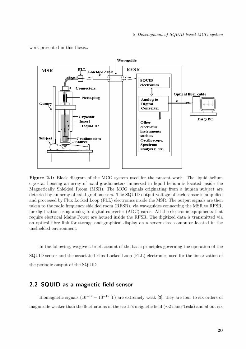
Figure 2.1: Block diagram of the MCG system used for the present work. The liquid heliumcryostat housing an array of axial gradiometers immersed in liquid helium is located inside theMagnetically Shielded Room (MSR). The MCG signals originating from a human subject aredetected by an array of axial gradiometers. The SQUID output voltage of each sensor is amplifiedand processed by Flux Locked Loop (FLL) electronics inside the MSR. The output signals are thentaken to the radio frequency shielded room (RFSR), via waveguides connecting the MSR to RFSR,for digitization using analog-to-digital converter (ADC) cards. All the electronic equipments thatrequire electrical Mains Power are housed inside the RFSR. The digitized data is transmitted viaan optical fibre link for storage and graphical display on a server class computer located in theunshielded environment.
In the following, we give a brief account of the basic principles governing the operation of the
SQUID sensor and the associated Flux Locked Loop (FLL) electronics used for the linearization of
the periodic output of the SQUID.
2.2 SQUID as a magnetic field sensor
Biomagnetic signals (10−12 − 10−15 T) are extremely weak [3]; they are four to six orders of
magnitude weaker than the fluctuations in the earth’s magnetic field (∼2 nano-Tesla) and about six
20
2 Development of SQUID based MCG system
to seven orders of magnitude weaker than the earth’s static magnetic field (∼50 µT). The magnetic
noise in an urban setting is generally caused by mains power line, vehicle movements, vibrations,
etc., which may be in the range 1 nano-Tesla to 100 nano-Tesla depending on the site. The
cardiac magnetic field (typically, ∼40 pT at the QRS peak) although relatively strong compared
to the magnetic field produced by the human brain (100 fT - 2 pT), is completely masked by the
ubiquitous ambient magnetic noise. In order to measure such a weak magnetic field associated with
the biomagnetic sources, there are two essential prerequisites;
• The first is a magnetic field sensor, which is sufficiently sensitive to measure such extremely
weak magnetic fields in the range of 100 femto-Tesla to 100 pico-Tesla.
• The second involves the reduction of the ambient magnetic noise to a level lower than the
signal of interest.
The advent of the Superconducting QUantum Interference Device (SQUID) [4, 5] with a sensitivity
of 1 to 10 femto-Tesla has therefore been crucial for the measurement and characterization of
biomagnetic fields; indeed, these are the only sensors with adequate sensitivity to measure the
biomagnetic fields.
Josephson effect and the flux quantization form the fundamental principles which govern the
operation of the SQUID [4, 5]. The flux quantization implies that the magnetic flux threading
through a closed superconducting loop is constrained to be an integral multiple of a flux quantum
(Φ0 = h2e , 1Φ0 = 2.07 × 10⁻¹⁵ Wb, where h is the Planck’s constant and e is the elementary
charge). Josephson effect refers to the establishment of phase coherence between two weakly coupled
superconductors, which allows super-current to flow from one superconductor to other without
developing any voltage. The weak coupling may be realized in practice by separating the two
superconductors by a thin tunnel barrier of an insulating material. Such a structure is known as
the Josephson junction, and the quantum mechanical tunneling of cooper pairs across the junction
assists in the establishment of phase coherence between the two superconductors.
Depending on the operating principle, SQUID sensors are broadly classified into two categories:
DC SQUID (which is biased with direct current) and RF SQUID (which uses a radio frequency
current bias). The DC SQUID consists of a superconducting loop intercepted by two weak links
21
2 Development of SQUID based MCG system
whereas in the RF SQUID, the superconducting loop is intercepted by a single weak link. Both
types of SQUID sensors act as magnetic flux to voltage transducers [4, 5] and their output voltage
is a periodic function of the magnetic flux coupled to them with the periodicity of a flux quantum
Φ0. SQUID sensors based on Nb (having transition temperature, Tc ∼9 K) are operated at liquid
helium temperatures (4.2 K) and are known as low Tc SQUIDs (LTSC SQUID), while SQUID
sensors based on high temperature superconductors such as YBCO (Tc ∼ 90 K) are operated at
liquid nitrogen temperatures (77 K) and are known as high-Tc SQUIDs (HTSC SQUID) [4]. LTSC
SQUID sensors offer superior sensitivities in the detection of magnetic field changes compared to the
HTSC SQUIDs. We use low temperature DC SQUID (based on Nb/AlOx/Nb Josephson junctions)
as a magnetic sensing device for MCG measurement and the working principle of the DC SQUID
is briefly discussed in the following section.
2.2.1 Working Principle
In the absence of any external magnetic field, when a symmetric DC SQUID (which has two
identical Josephson junctions) is biased with a DC current (Ib), the bias current Ib divides equally
(I1 = I2 = Ib/2) into the two branches as shown in fig.2.2(a) and flows through the two Josephson
junctions. The critical current (which represents the maximum current the SQUID sensor can
support at zero voltage) of the SQUID in this case would be equal to 2Ic, where Ic denotes the
critical current of each Josephson junction. When a magnetic field (B) is applied perpendicular
to the plane of the SQUID loop, a screening current (Is) begins to circulate around the loop so
as to produce the necessary magnetic flux required to satisfy the requirement of flux quantization
[4, 5, 6].
Φtot = Φext + LIs = nΦ0 (2.1)
Here Φtot is the total flux threading the SQUID loop, Φext is the externally applied flux, Is is the
screening current induced by the applied flux, n is an integer which has to be chosen to minimize
Is, L is the inductance of the SQUID loop, and Φ0 is the flux quantum. When the external applied
flux is nΦ0, the screening current Is induced is zero and when the external applied flux is (n+ 12)Φ0,
the induced screening current is ±(Φ0/2L). Thus, as the magnetic flux coupled to the SQUID is
monotonically varied, the induced screening current varies periodically with the periodicity of Φ0.
22
2 Development of SQUID based MCG system
Since the induced current circulates around the SQUID loop in a clockwise or counterclockwise
direction depending on the magnitude and direction of the applied magnetic field, the direction
of the induced current Is is the same as that of the bias current Ib in one branch of the SQUID
while its direction is opposite to that of the bias current in the other branch, and this gives rise
to a total current of I1(= Ib2 + Is) in one branch while in other branch, it is I2(= Ib
2 − Is) (see
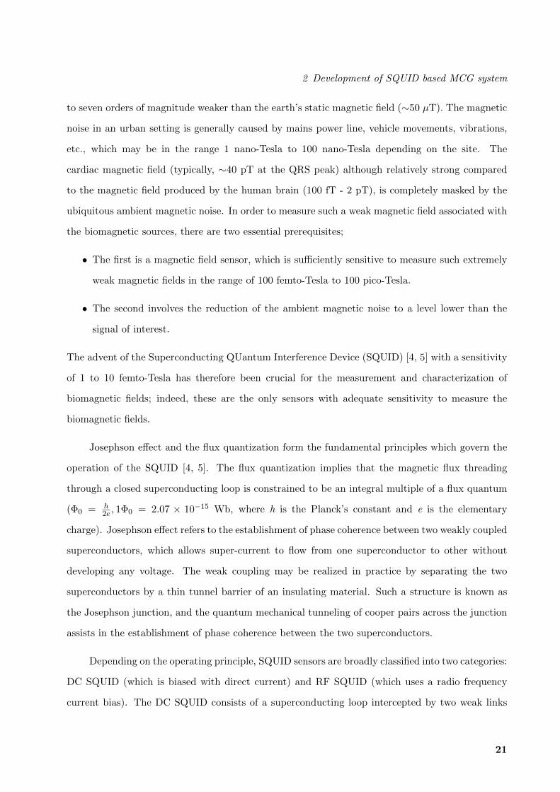
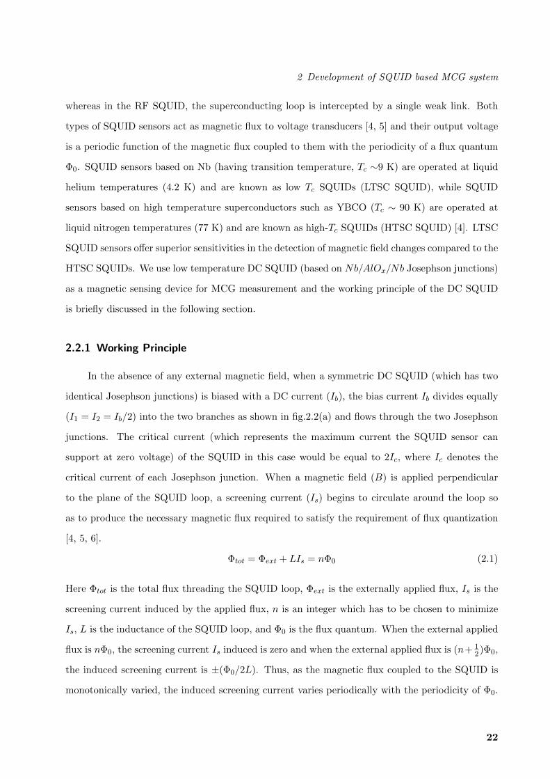
fig.2.2(a)). A voltage appears across the junction as soon as the total current in any one of the
(a) (b)
Figure 2.2: (a) The schematic of the DC SQUID sensor (b) Periodic variation of the output voltageof the SQUID with the periodicity of a flux quantum (Φ0), as the magnetic flux threading throughthe SQUID is monotonically varied (known as the V − Φ characteristic of SQUID) (adapted from[5]). Normally, SQUID is locked at the operating point W, and the effect of any applied magneticflux is compensated by an equivalent feedback flux to lock the SQUID at the operating point. Anyexcursions around the operating point are limited to a very small region around W over which theV − Φ characteristic is linear with a flux-to-voltage transfer function of the bare SQUID sensorgiven by the slope (VΦ = ∂V/∂Φ).
two branches exceeds the critical current of the Josephson junction in that branch. As a result of
this, the critical current of the SQUID reduces from 2Ic to (2Ic − 2Is). The critical current of the
SQUID is a periodic function of the externally applied magnetic flux and is given by [7].
Icmax(Φext) = 2Ic|cos(πΦext
Φ0)| (2.2)
A voltage is developed across the SQUID when the SQUID is biased with DC current slightly larger
than 2Ic; this output voltage is a periodic function of external flux with the periodicity of a flux
23
2 Development of SQUID based MCG system
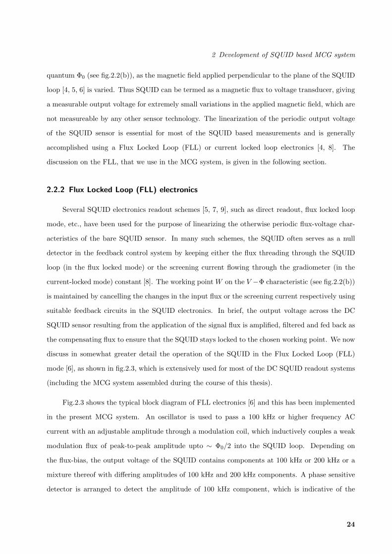
quantum Φ0 (see fig.2.2(b)), as the magnetic field applied perpendicular to the plane of the SQUID
loop [4, 5, 6] is varied. Thus SQUID can be termed as a magnetic flux to voltage transducer, giving
a measurable output voltage for extremely small variations in the applied magnetic field, which are
not measureable by any other sensor technology. The linearization of the periodic output voltage
of the SQUID sensor is essential for most of the SQUID based measurements and is generally
accomplished using a Flux Locked Loop (FLL) or current locked loop electronics [4, 8]. The
discussion on the FLL, that we use in the MCG system, is given in the following section.
2.2.2 Flux Locked Loop (FLL) electronics
Several SQUID electronics readout schemes [5, 7, 9], such as direct readout, flux locked loop
mode, etc., have been used for the purpose of linearizing the otherwise periodic flux-voltage char-
acteristics of the bare SQUID sensor. In many such schemes, the SQUID often serves as a null
detector in the feedback control system by keeping either the flux threading through the SQUID
loop (in the flux locked mode) or the screening current flowing through the gradiometer (in the
current-locked mode) constant [8]. The working point W on the V −Φ characteristic (see fig.2.2(b))
is maintained by cancelling the changes in the input flux or the screening current respectively using
suitable feedback circuits in the SQUID electronics. In brief, the output voltage across the DC
SQUID sensor resulting from the application of the signal flux is amplified, filtered and fed back as
the compensating flux to ensure that the SQUID stays locked to the chosen working point. We now
discuss in somewhat greater detail the operation of the SQUID in the Flux Locked Loop (FLL)
mode [6], as shown in fig.2.3, which is extensively used for most of the DC SQUID readout systems
(including the MCG system assembled during the course of this thesis).
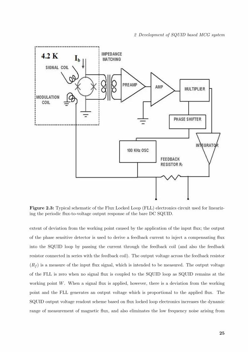
Fig.2.3 shows the typical block diagram of FLL electronics [6] and this has been implemented
in the present MCG system. An oscillator is used to pass a 100 kHz or higher frequency AC
current with an adjustable amplitude through a modulation coil, which inductively couples a weak
modulation flux of peak-to-peak amplitude upto ∼ Φ0/2 into the SQUID loop. Depending on
the flux-bias, the output voltage of the SQUID contains components at 100 kHz or 200 kHz or a
mixture thereof with differing amplitudes of 100 kHz and 200 kHz components. A phase sensitive
detector is arranged to detect the amplitude of 100 kHz component, which is indicative of the
24
2 Development of SQUID based MCG system
Figure 2.3: Typical schematic of the Flux Locked Loop (FLL) electronics circuit used for lineariz-ing the periodic flux-to-voltage output response of the bare DC SQUID.
extent of deviation from the working point caused by the application of the input flux; the output
of the phase sensitive detector is used to derive a feedback current to inject a compensating flux
into the SQUID loop by passing the current through the feedback coil (and also the feedback
resistor connected in series with the feedback coil). The output voltage across the feedback resistor
(Rf ) is a measure of the input flux signal, which is intended to be measured. The output voltage
of the FLL is zero when no signal flux is coupled to the SQUID loop as SQUID remains at the
working point W . When a signal flux is applied, however, there is a deviation from the working
point and the FLL generates an output voltage which is proportional to the applied flux. The
SQUID output voltage readout scheme based on flux locked loop electronics increases the dynamic
range of measurement of magnetic flux, and also eliminates the low frequency noise arising from
25
2 Development of SQUID based MCG system
low frequency drifts in the junction critical currents/other SQUID parameters and 1/f noise from
the preamplifiers etc. as the signal of interest is moved to frequencies (∼100 kHz) above the 1/f
threshold. Since the maximum feedback voltage is limited by the supply voltage (say, 12 V), the
dynamic range is limited to the flux equivalent of the supply voltage at the selected gain of FLL
and may be increased depending on the requirements by selecting a lower FLL gain, which may be
easily tuned by changing the feedback resistor Rf , since it is given by the ratio Rf/Mf . The output
voltage that appears across the feedback resistor Rf is proportional to the external flux intended
to be measured and thus the periodic response of the bare SQUID is converted into a linear one,
with a flux-to-voltage conversion factor independent of the open loop gain of the amplifier [10].
Although, the signal bandwidth is limited by the modulation frequency and is often sub-
stantially lower than the modulation frequency, this is not a serious limitation in biomagnetic
investigations since a bandwidth of 1kHz is adequate for most of the applications. In the FLL
mode, the total magnetic flux noise of the dc SQUID is given by [7],
S12Φ =
√SΦ,SQUID +
SV,AMPL
V 2Φ
(2.3)
where SΦ,SQUID and SV,AMPL are the flux noise of the SQUID and voltage noise of the preamplifier
respectively and VΦ(= ∂V/∂Φ) is the flux-to-voltage transfer function of the bare SQUID. It may
be noted that the decrease in the flux-to-voltage transfer function VΦ deteriorates the attainable
signal-to-noise ratio.
2.3 Reduction of ambient magnetic noise
Although SQUID sensors have the requisite sensitivity to detect the extremely weak bio-
magnetic fields, the ambient magnetic noise such as that associated with power line interference,
vibrational noise, magnetic noise associated with vehicle movements etc., present at the site is
orders of magnitude higher than the signal of interest and completely masks it. This poses a real
difficulty in the measurement of biomagnetic signals, unless the ambient magnetic noise in the
frequency bandwidth of interest (0-1000 Hz) is suppressed to a sufficiently low level.
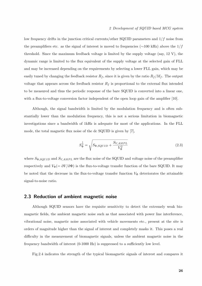
Fig.2.4 indicates the strength of the typical biomagnetic signals of interest and compares it
26
2 Development of SQUID based MCG system
with the strength of the magnetic fields associated with some of the parasitic sources of ambient
magnetic noise in the neighbourhood [7, 12]. In order to detect such extremely weak biomagnetic
Figure 2.4: Schematic illustration of the strength of the magnetic fields originating from differentsources (adapted from [12]). Since the biomagnetic fields of interest are much weaker compared tothe parasitic ambient magnetic noise, it is essential to attenuate the ambient magnetic noise usingsome form of shielding in order to measure the signal of interest.
signals, it is therefore essential to attenuate all the parasitic sources of the ambient magnetic
noise by using some form of shielding [7, 13] such as that provided by a Magnetically Shielded
Room (MSR) and by using pick-up loops in the form of gradiometers [14] which further reduce the
contribution of the residual magnetic noise present inside the MSR by discriminating against distant
sources of magnetic noise which are expected to produce a nearly uniform field over the relatively
small volume of the gradiometer; nearby sources, on the other hand, are expected to produce
a non-uniform magnetic field over the volume of the gradiometer and, hence, get preferentially
detected. Some research groups have tried to avoid the use of the expensive MSR for biomagnetic
measurements by using higher order hardware gradiometers [14] or synthetic gradiometers [15] for
measuring biomagnetic signals in an unshielded environment; however, measured signals in this
case are generally of much poorer quality. In the following sections, we discuss the basics of MSR
and the gradiometers that we employed for the reduction of ambient magnetic noise.
27
2 Development of SQUID based MCG system
2.3.1 Magnetically Shielded Room (MSR)
As discussed earlier, Magnetically Shielded Room (MSR) is a prerequisite for biomagnetic
measurements and is of crucial importance for all high quality measurements of biomagnetic sig-
nals [7, 11, 16]. MSR serves to attenuate the external ambient magnetic noise to a sufficiently
low level so as to enable the SQUID sensors to measure the extremely weak biomagnetic signals,
which are otherwise completely masked by the ambient magnetic noise. The magnetic shielding
may be categorized into various types: ferromagnetic shielding using high permeability µ-metal
(low frequency magnetic shielding), eddy current shielding using high conductivity aluminum or
copper [7](high frequency magnetic shielding), active compensation [17] or superconducting mag-
netic shielding [18] etc. Here, we specifically describe the shielding configuration employed in our
laboratory [19].
Our Magnetically Shielded Room (MSR), custom built by IMEDCO, Switzerland, inside which
all the measurements reported in this thesis were carried out, has the internal dimensions 3m(width)
× 4m(length) × 2.4m(height) and is constructed using two layers of ferromagnetic shielding (µ-
metal) and two layers of eddy current shielding (aluminum) on each of the six sides. The outer
aluminum layer is 4 mm thick, while the outer µ-metal layer is 2 mm thick. The inner aluminum
layer is 8 mm thick while the inner µ-metal layer is 3 mm thick. The top panel of fig.2.5 shows the
photograph of the MSR erected in our laboratory, at IGCAR, for biomagnetic measurements such
as MCG and MEG. The principles of magnetic shielding provided by µ-metal and the aluminum
layer may be explained [5, 11, 16] as follows:
High frequency magnetic noise is attenuated through the induction of eddy currents in the
grounded high conductivity aluminum panels; by Lenz’s law the eddy currents are induced in a
direction so as to oppose the original magnetic field fluctuations. While this eddy current shielding is
quite effective at high frequencies, it ceases to be effective at low frequencies owing to an inevitable
increase in skin depth at low frequencies. For low frequency magnetic shielding, ferromagnetic
materials such as µ-metal are used for the construction of the walls of MSR. Owing to the very high
magnetic permeability of the µ-metal compared to air, it offers a path of low magnetic reluctance to
the magnetic lines of force, and consequently, the magnetic field lines, which would have otherwise
28
2 Development of SQUID based MCG system
(a)
(b)
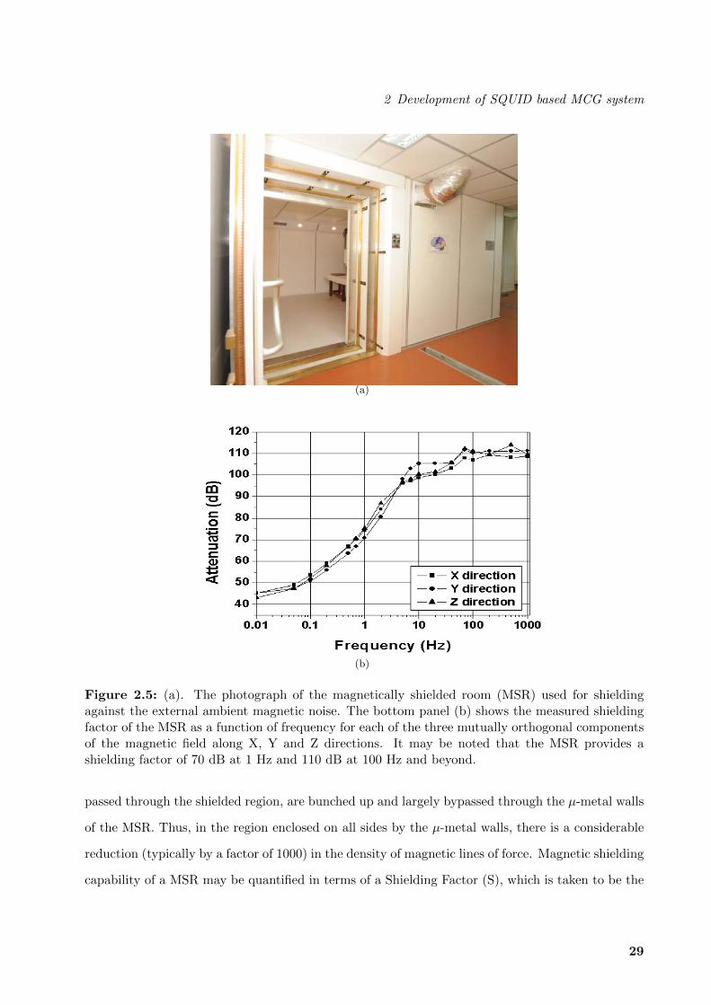
Figure 2.5: (a). The photograph of the magnetically shielded room (MSR) used for shieldingagainst the external ambient magnetic noise. The bottom panel (b) shows the measured shieldingfactor of the MSR as a function of frequency for each of the three mutually orthogonal componentsof the magnetic field along X, Y and Z directions. It may be noted that the MSR provides ashielding factor of 70 dB at 1 Hz and 110 dB at 100 Hz and beyond.
passed through the shielded region, are bunched up and largely bypassed through the µ-metal walls
of the MSR. Thus, in the region enclosed on all sides by the µ-metal walls, there is a considerable
reduction (typically by a factor of 1000) in the density of magnetic lines of force. Magnetic shielding
capability of a MSR may be quantified in terms of a Shielding Factor (S), which is taken to be the
29
2 Development of SQUID based MCG system
ratio of the external field (HA) outside the MSR to the corresponding residual field (HR) in the
interior of the MSR; since the attenuation is frequency dependent, the Shielding Factor varies with
frequency [20]. It is usual to express the Shielding Factor of a MSR on a logarithmic scale (dB) as
per eq. 2.4:
S = 20log(HA
HR) (2.4)
The bottom panel of fig.2.5 shows the shielding performance of the MSR as a function of frequency
for all the three mutually orthogonal components of magnetic field. MSR provides a shielding factor
of 70 dB at 1 Hz, which steadily improves to 110 dB at 100 Hz and beyond as seen in fig.2.5(b).
MSR is equipped with a pneumatically operated door and four waveguides to route the SQUID
cables without noise pick up from the ambient into an adjoining Radio Frequency Shielded Room
(RFSR), which houses the electronic instrumentation.
2.3.2 SQUID Gradiometers
For coupling the signal of interest into the sensing area of the SQUID, a superconducting flux
transformer is conventionally used to enhance the attainable field sensitivity. The superconducting
flux transformer typically consists of either a single superconducting pickup loop (magnetometer)
or a set of superconducting pick-up loops connected in opposition (gradiometer); it serves to sense
the instantaneous net magnetic flux at its location and couple it to the input coil of the SQUID
so that the SQUID sensor generates a proportional voltage output. Gradiometer type of pick-up
loops have emerged as the preferred flux transformer design inside most MSRs which provide only
a moderate level of attenuation of ambient magnetic noise (40 dB to 80 dB) and, despite their
somewhat lower sensitivity for the detection of deeper sources, offer the advantage of additional
attenuation of contributions arising from distant sources of noise.
In the gradiometer configuration, the coil which is closer to the source of interest is known as
the pickup coil and the other coils which are away from the source are known as the compensation
coils. The first order gradiometer is obtained by separating a pickup coil and a compensation coil
by a distance called the baseline of the gradiometer. The gradiometers may be classified as axial
or planar depending on the spatial gradient of the magnetic field sensed by them. The axial gra-
30
2 Development of SQUID based MCG system
diometer measures the spatial gradient of the magnetic field along the axial direction perpendicular
to the pick-up loop (∂Bz/∂z) and the off-diagonal or planar gradiometers measure the spatial gra-
dient along the two orthogonal directions in the plane of the pick-up loop (∂Bz/∂x, ∂Bz/∂y). Such
gradiometers are commonly referred to as hardware gradiometers [7, 11], as distinct from synthetic
gradiometers [14, 15, 16] which can be constructed electronically [13] or using software [15]. In
the synthetic gradiometers, output signals of the lower order gradiometers are readout separately
and subtracted. The different types of gradiometer configurations used conventionally in a SQUID
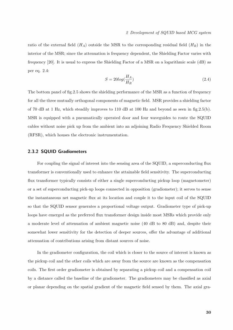
based measuring set-up are illustrated in fig.2.6.
Figure 2.6: Schematic illustration of different types of pick-up coils used in a SQUID basedmeasuring set-up (adapted from [4]). (a) to (e) show the different types of pick-up coils such as themagnetometer, first order axial gradiometer, second order axial gradiometer, planar gradiometerin the x-direction and planar gradiometer in the y-direction respectively. The magnetometer (a)measures the total magnetic field produced by both the signal of interest and any nearby as well asdistant sources of magnetic noise. The gradiometers (b,c,d and e) measure the spatial gradient ofthe magnetic field (∂Bz/∂z, ∂
2Bz/∂z2, ∂Bz/∂x, ∂Bz/∂y respectively for (b)-(e)), and are relatively
insensitive to distant sources of magnetic noise.
A first order axial gradiometer (used in our MCG system) consists of two equal radius loops of
superconducting wire separated along the common axis by a distance b (baseline of the gradiometer,
which is typically 5 cm in our system) and wound in opposition (one loop is clockwise while the
other loop is anti-clockwise). Since the gradiometer basically senses the difference in magnetic flux
31
2 Development of SQUID based MCG system
threading through the two oppositely wound pick-up loops, the output of an ideally balanced gra-
diometer is zero if the applied magnetic field is uniform over the region occupied by the gradiometer.
The variation of attenuation with the source distance R is governed by the parameter (b/R)2 for a
first order axial gradiometer. The immunity of the gradiometer to the external sources of ambient
magnetic noise can be further improved by using higher order gradiometers which comprise of two
or more lower order gradiometers connected in opposition (which are designed to sense higher order
spatial derivatives of the magnetic field); indeed using second or higher order gradiometers, some
research groups have succeeded in measurement of biomagnetic fields in an unshielded environment,
although the quality of the measured data is relatively poor.
2.4 MCG system modules
As some of the modules of MCG system such as SQUID gradiometers, MSR, and FLL elec-
tronics have been already discussed in the earlier sections, we now describe the remaining modules
of the MCG system in the subsequent sections.
2.4.1 MCG cryostat and the SQUID insert
The SQUID sensors have to be operated at a temperature well below the superconducting
transition temperature of the superconducting materials used for their fabrication. Niobium has
a superconducting transition temperature of ∼9 K, and hence, LTSC SQUID sensors based on
niobium (that we use) are usually operated by immersing them in liquid helium, which has a
boiling point of 4.2 K at the normal pressure of 1 atm., and, hence, provides a stable thermal
environment for the operation of the SQUID sensor. For storing cryogenic liquids such as liquid
helium or liquid nitrogen, it is necessary to use a cryostat or a dewar, which is specially designed
to reduce heat leaks associated with thermal conduction, convection and radiation and achieve a
reasonably low boil-off rate and consequently a longer holding time [5, 16, 20].
The MCG measurements are carried out inside a MSR housing the liquid helium cryostat
in which SQUIDs are immersed in liquid helium in order to operate them at the temperature of
4.2 K. The cryostat is supported on a non-magnetic gantry, which allows the cryostat to be moved
32
2 Development of SQUID based MCG system
vertically, along the z-axis, in order to adjust its position above the thorax of the subject, depending
on the experimental needs. As mentioned earlier in the section 2.1, the MCG system at IGCAR
was progressively upgraded from a single channel system developed initially to the 37 channels
system presently operational. Each SQUID channel consists of an axial gradiometer connected to a
DC SQUID, a flux-locked-loop module, an Analog-to-Digital Converter (ADC) module to digitize
the data, which is eventually displayed on a computer as the channel output as a function of time.
While the individual modules (or units) of the MCG system are identical for MCG systems with
different number of channels, there are variations in the overall size of the fiber reinforced plastic
(FRP) cryostat, the number of SQUID gradiometers, inter-sensor spacing, the number of channels
in the data acquisition system hardware etc. The increase in size of the cryostat is necessary to
accommodate a larger number of sensors with a view to increase the area covered by the sensors
over the surface of the thorax. Table 2.1 shows the features of the different MCG systems developed
during the course of this thesis; in each system, different cryostats and sensor configurations were
used. The photographs of the 4 channel and 13 channel MCG systems have been respectively
shown in fig.2.7 and fig.2.8(a), while a dimensioned sketch of the 37 channel cryostat is shown in
fig.2.9(a).
Table 2.1: The different MCG systems which were developed during the course of this thesis work.The cryostat used for the single channel system was also used for the four channel system. Whilethe individual modules (or units) of the MCG system are identical for MCG systems with differentnumber of channels, there are variations in the overall size of the fiber reinforced plastic (FRP)cryostat, the number of SQUID gradiometers, inter-sensor spacing, the number of data acquisitionchannels etc.
No. ofchannels
Liquid heliumcapacity (litres)
Warm-to-colddistance (mm)
Area covered onthorax (cm2)
LHe boil-offrate (litres/day)
Geometry ofsensor array
Inter-Sensorspacing(mm)
4 11.5 10 40 2 square 42
13 13 10 106 3 hexagonal 28
37 18 16 300 5 hexagonal 30
The single channel and four channel MCG systems were assembled in a 11.5 litre capacity
liquid helium cryostat, while the 13 channel system and the 37 channel system were assembled in
liquid helium cryostats having a capacity to hold 13 and 18 litres of liquid helium respectively. The
33
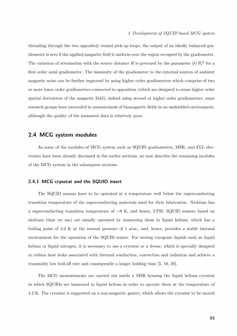
2 Development of SQUID based MCG system
Figure 2.7: The photograph of the 4 channelMCG system developed during the course ofthis thesis. The inset in the photograph showsthe SQUID holder in which the first order ax-ial gradiometers are housed in a square latticewith an inter-sensor spacing of 42 mm.
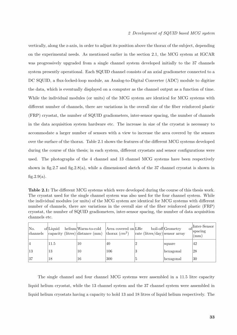
(a) (b)
Figure 2.8: (a) The photograph of the 13 channel MCG system developed during the course ofthis thesis. The inset in the photograph shows the SQUID holder in which the first order SQUIDaxial gradiometers are arranged in a hexagonal lattice with an inter-sensor spacing of 28 mm. (b)The photograph of the top view of the 13 channel cryostat showing the recesses (for locating thesensors) provided on the bottom plate of the liquid helium vessel of the cryostat, which serve toreduce the warm-to-cold distance.
holding time of liquid helium depends on the evaporation rate and the latter is listed for MCG
systems with different number of channels. The geometrical configuration of the sensors and the
34

2 Development of SQUID based MCG system
inter-sensor spacing which eventually determine the coverage area are also different for the different
MCG systems.
(a) (b)
Figure 2.9: (a) A dimensioned schematic sketch of the 37 channel MCG cryostat. The portionenclosed by the oval at the bottom of (a) is enlarged at right to show the warm-to-cold distancewhich is about 16 mm. (b) The sketch of the top view of the 37 channel cryostat showing therecesses (for locating the sensors) provided on the bottom plate of the liquid helium vessel of thecryostat, which serve to reduce the warm-to-cold distance.
It is important for a MCG cryostat to have the warm-to-cold distance as low as possible so that
the pick-up coil of the sensors at liquid helium temperatures could be brought as close as possible
to the skin surface of the subject, which has to be at room temperature. To ensure this, each
cryostat is provided with recesses on the bottom plate of the liquid helium vessel at the locations of
the sensors so that each sensor would be actually fitted to sit inside the appropriate recess so that
the respective pick-up coil is as close as possible to skin surface. Fig.2.8(b) and 2.9(b) respectively
show the photograph and sketch of the top view of the 13 channel and 37 channel cryostats. The
recesses can be seen at the bottom flange of the liquid helium vessel of the cryostat which serve to
reduce the warm-to-cold distance. Since the magnetic field decreases rapidly as one moves away
from the source, it is important that the sensors are as close to the source as possible so that the
measurements are performed with a relatively high signal-to-noise ratio. Reduction of the stand-
off distance between the warm and cold surfaces of the cryostat to values ∼10 mm leads to an
35

2 Development of SQUID based MCG system
improved signal-to-noise ratio [19]. The warm-to-cold distance is about 10 mm for the four and
thirteen channel cryostats whereas, for the 37 channel cryostat, it is about 16 mm.
With cryostats having a lower number of channels, it was necessary to perform sequential
measurements in multiple configurations of sensor positions over the thorax in order to cover the
thoracic area of interest for MCG measurements with consequent uncertainties in sensor positions
as well as the considerably long time required to complete a typical MCG scan; when the 37 channel
system became operational, it was possible to record the MCG signals simultaneously over an array
of 37 points arranged on a hexagonal lattice covering a much larger area (300 cm2) on the anterior
surface of the thorax, and the need to perform sequential measurements was obviated, making the
MCG scans relatively faster. With the 37 channel cryostat, sensor positions were also accurately
known, leading to a much smaller uncertainty in the coordinates of the sensors during the MCG
measurement, thereby enhancing the reproducibility [21] of the MCG data recorded during different
experimental runs; consequently, the error in the reconstruction of the source from the measured
MCG data is also considerably lower [22].
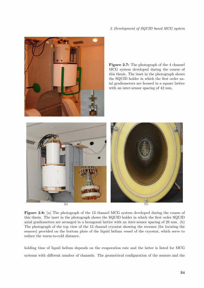
A suitable insert was designed for each cryostat along with a SQUID holder on which the
SQUID modules, comprising of the wire wound axial gradiometer coupled to a SQUID sensor, were
mounted. The SQUID insert fabricated from the fiber-reinforced plastic (FRP) material, which goes
inside the cryostat, is equipped with a set of mounting plates to support the SQUID gradiometers
at the bottom and the insulated LEMO electrical connectors (which are used to connect the SQUID
electrical leads) at the top [19]. Each axial gradiometer consisted of two superconducting loops of
15 mm diameter separated by a baseline of 50 mm and was connected via superconducting contacts
to the input coil which was integrated on-chip. The insert is also equipped with suitable radiation
baffles in the neck region, to reduce the boil-off of liquid helium as a consequence of radiative heat
leak. Fig.2.10 shows the photographs of the insert. The SQUID insert and the SQUID holder are
designed in such a way that as the insert is carefully lowered into the cryostat, each gradiometer
sits snugly into the corresponding 10 mm deep recess specially provided on the bottom flange of
the liquid helium vessel in order to bring the pick up loop of the gradiometer as close to the source
as possible.
36
2 Development of SQUID based MCG system
Figure 2.10: Photograph of the insert ofthe 37 channel MCG system which comprisesof electrical connectors, SQUID holders, ra-diation baffles, mounting plates, etc. Thefirst order axial gradiometers are mountedon the SQUID holder on a hexagonal lat-tice with inter-sensor spacing of 30 mm.This whole assembly is inserted inside the37 channel cryostat.
2.4.2 SQUID electrical leads
An Electro-Static Discharge (ESD) safe work bench and ESD safe work-practices were used
during the assembly of the SQUID sensors onto the SQUID insert, to avoid the risk of any possible
damage to the tunnel barriers of the SQUID sensor by electrostatic discharge during mounting of
the sensors and soldering of the electrical leads. Each SQUID module was wired with four twisted
pairs of electrical leads, one pair each for bias current, flux modulation, SQUID output voltage
and heater. The use of twisted pairs of electrical leads offers substantial immunity against the
possible contamination of the signal by inductively coupled noise. The 40 SWG low resistive (∼
1 Ωm−1) copper wires were used for voltage and bias leads of the SQUID, while 40 SWG high
resistive (∼ 35 Ωm−1) manganin wires were used for the modulation and heater leads. The use
of low resistive copper wires for the SQUID output voltage reduces the possibility of any signal
drop across the electrical leads [23], especially when the relatively low output impedance of the
SQUID sensor (∼ 1 Ω) is transformed using an impedance matching transformer to the values of
source impedance at which the preamplifier yields the best noise performance. Use of low thermal
conductivity manganin wires [23] for the other electrical leads (modulation and heater) serves to
minimize the heat leak into the cryostat and consequently contributes to reducing the boil-off of
liquid helium, thereby increasing the hold-time of the cryostat. The heater incorporated in the
37
2 Development of SQUID based MCG system
sensor is occasionally used in case magnetic flux is accidentally trapped in the form of vortices in
the vicinity of the Josephson junctions constituting the SQUID sensor and consequently, the critical
current of the SQUID as well as the modulation depth of the SQUID are reduced. In such a case,
the heater may be activated for a few seconds to pass a current to raise the temperature of the
SQUID sensor above the superconducting transition temperature Tc, in order to detrap the trapped
flux and restore the critical current as well as the modulation depth to their original values, in the
cool down of the SQUID on switching off the heater. The SQUID output voltage signals from all
the channels, which are first routed to the intermediate electrical connectors on the mounting plate
of the insert, are eventually brought out of the cryostat to the electrical connectors at the top of the
insert by means of twisted pairs of electrical leads [2]. The battery powered modules comprising of
preamplifier and the FLL electronics are located close to the top of the cryostat.
2.4.3 Radio Frequency Shielded Room (RFSR)
The linearized FLL output voltages from all the SQUID channels are routed via shielded cables
through the waveguides connecting the MSR to an adjoining Radio Frequency Shielded Room
(RFSR) [19], where necessary electronic instrumentation for analog-to-digital conversion (ADC)
and data acquisition is located. The RFSR houses all the electronic instrumentation requiring the
Mains Power such as the control units for the FLL, ADC modules to digitize the SQUID output
voltage signal in each channel, function generators, oscilloscope, spectrum analyzer and other test
and measuring instrumentation required during an experiment. Fig.2.11(a) shows a photograph
of the RFSR and shows how it is connected to the MSR via four 100 mm diameter waveguides,
while fig.2.11(b) shows a photograph of the electronic instrumentation housed inside the RFSR.
The RFSR is constructed using 2 mm thick aluminum sheets of high electrical conductivity and
provides a shielding factor of 100 dB at frequencies of 1 MHz and beyond [19].
The digitized voltage output data from all the SQUID channels is transmitted outside the
RFSR over a fiber optic cable to a data acquisition system PC (DAQ-PC) located in the unshielded
area through a port provided for this purpose on the rear wall of the RFSR. The fiber optic
cable supports data transfer rates upto 75 Mbps and provides immunity against noise during the
transmission of data to PC. The RFSR is equipped with ten signal line feedthrough filters, which
38

2 Development of SQUID based MCG system
(a) (b)
Figure 2.11: (a). The photograph of the Radio Frequency Shielded Room (RFSR) coupled to theMagnetically Shielded Room via four waveguides (left panel). The right panel shows a view of theelectronic instruments kept inside the RFSR. The RFSR provides high frequency shielding againstelectromagnetic interference with an attenuation factor of 100 dB at 1 MHz and beyond.
allows the passage of low level, low frequency signals inside RFSR, if desired by the user. All the
electronic instruments inside the RFSR derive the Mains Power from a special isolation transformer,
located far away from the MSR and RFSR, and the 220V, AC power line enters the RFSR via a
filter.
2.4.4 Data Acquisition System
Based on the experimental requirements, the SQUID output voltage signal in each channel,
which is proportional to the instantaneous axial gradient ∂Bz/∂z at the location of the gradiometer,
may be low pass filtered with user desired cut-off frequency which may be set at any of the four
values: 30 Hz, 100 Hz, 300 Hz and 1 kHz. An individual Delta-Sigma ADC is used for digitizing
the SQUID output voltage in each channel with a 24 bit resolution at any user desired sampling
rate upto 200 kHz [19]. However it may be noted that for most measurements a sampling rate of
1 kHz is adequate. The digitized data received over the optical fibre link is stored in a server PC,
which is equipped with a custom-built data acquisition and display software. The software, based
on a LABVIEW platform enables real-time graphical display of the output voltage of each channel
39
2 Development of SQUID based MCG system
as a function of time, with modules for low-pass, high-pass or band-pass filtering depending on
the needs of the user. Besides allowing the data to be visualized in the time domain, the software
enables investigations of the spectral content in the frequency domain and is also equipped with
modules required for trigger based epoching and averaging to suppress uncorrelated noise, which
are important for studies of evoked response in the context of MEG and for visualizing weak effects
such as those associated with the activation of His bundle in Signal Averaged MCG (SAMCG).
The channel output data, together with information on the experimental details and the sensor
coordinates, is stored in the computer for subsequent off-line analysis.
2.5 Field gradient-to-Voltage Calibration for SQUID gradiometer
The SQUID system needs to be properly calibrated, prior to the biomagnetic measurements so
that the measured SQUID output voltage may be expressed in terms of magnetic field, or magnetic
field gradient using the calibration factor. For calibration, it is customary to relate the output
voltage of the magnetometer or gradiometer to the value of the external magnetic field or field
gradient produced by a known reference system. In general, the calibration factor is expressed as
voltage/field or as voltage/field gradient. It is important that the calibration factor is accurately
known in a multichannel biomagnetic system, since even a few percent error in calibration may
result in appreciable errors in the source localization [22]. Although several calibration procedures
have been reported in the literature [20, 24], we have adopted relatively a simple procedure for
calibrating the output voltage of the SQUID sensors, which is found to be effective.
We used a large circular current carrying coil, encircling the tail of the Dewar, whose diameter
was 20 times larger than the diameter of the superconducting gradiometer coil, which was used for
sensing the magnetic field (or field gradient) and coupling it to the SQUID sensor as a proportional
flux. In this arrangement, the coil is aligned to be along the gradiometer axis and its position
is adjusted until a maximum voltage from the SQUID is obtained. From Biot-Savart’s law, the
vertical component of the magnetic field Bz at a distance z from the centre along the axis of the
large circular coil is given by [24],
Bz(x = 0, y = 0, z) =µ0NIa
2
2(a2 + z2)3/2(2.5)
40
2 Development of SQUID based MCG system
where, N is the number of turns in the large circular coil, I is the current passed through the coil,
a is the radius of the large circular coil and z is the distance between the sensor and the coil along
the vertical axis. One can change either the amplitude of the current I by adjusting the level of
the sinusoidal voltage in the signal generator or the vertical distance z by adjusting the height of
the cryostat vertically to vary the input magnetic field values and the output voltage of the SQUID
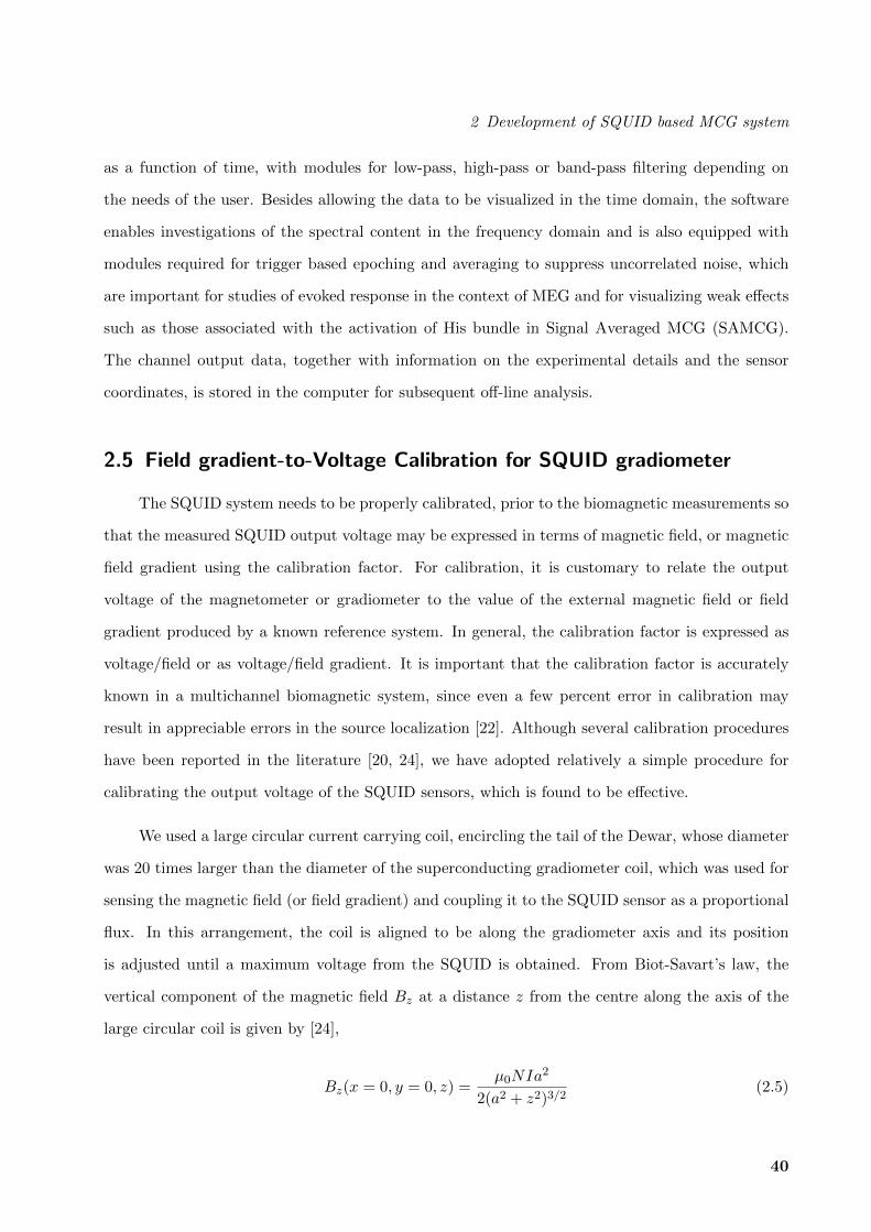
for the corresponding changes in the magnetic field are recorded. As the sensor used was a first
order axial gradiometer, the first order derivative of Bz at the sensor position is evaluated and the
observed SQUID output voltage is plotted against the known value of the field gradient ∂Bz/∂z as
shown in fig.2.12. The slope of the calibration plot yields the calibration factor. For instance, we
estimated the calibration factor for the first order axial gradiometer, with a loop diameter of 15
mm and a baseline of 50 mm, as 22.2 pT/cm/V.
Figure 2.12: The flux-to-voltagecalibration plot for a typical SQUIDsensor. A known value of mag-netic field (or field gradient) is pre-sented to the sensor by passinga known amplitude of sinusoidallyvarying current through a large cir-cular coil and the amplitude of theflux-locked-loop (FLL) output volt-age for the corresponding magneticfield (or field gradient) is recorded.FLL output voltage is recorded fordifferent values of applied magneticfield (or field gradient). The slope ofthe plot of FLL output as a functionof applied magnetic field (or fieldgradient) is taken to be the calibra-tion factor, which is used for con-verting the measured SQUID outputvoltage into the corresponding mag-netic field (or field gradient).
2.6 Field gradient noise level in the SQUID system
It is imperative that, for a signal of interest to be measurable, its amplitude should be much
larger than the sensitivity of the sensor used in the required bandwidth and the latter is limited
41
2 Development of SQUID based MCG system
by the intrinsic noise generated within the SQUID sensors and the extrinsic noise associated with
electronics units, residual ambient magnetic noise, vibrations etc [20]. Hence, the background noise
(the environmental noise in the absence of the subject) measured in the shielded room with an
axial gradiometer must be lower than the signal of interest and this condition implies that white
noise level of the sensor should not be more than several fTrms/cm/√Hz which represents the
typical spectral density of the noise content in unit frequency bandwidth. The minimum noise level
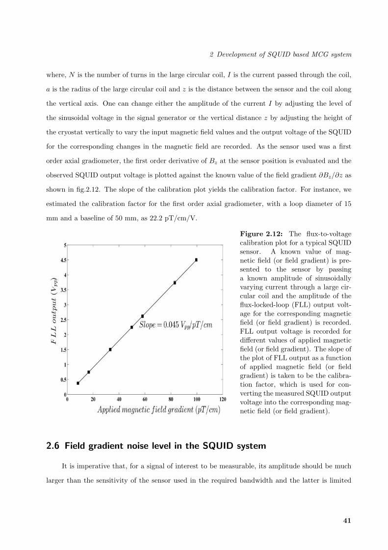
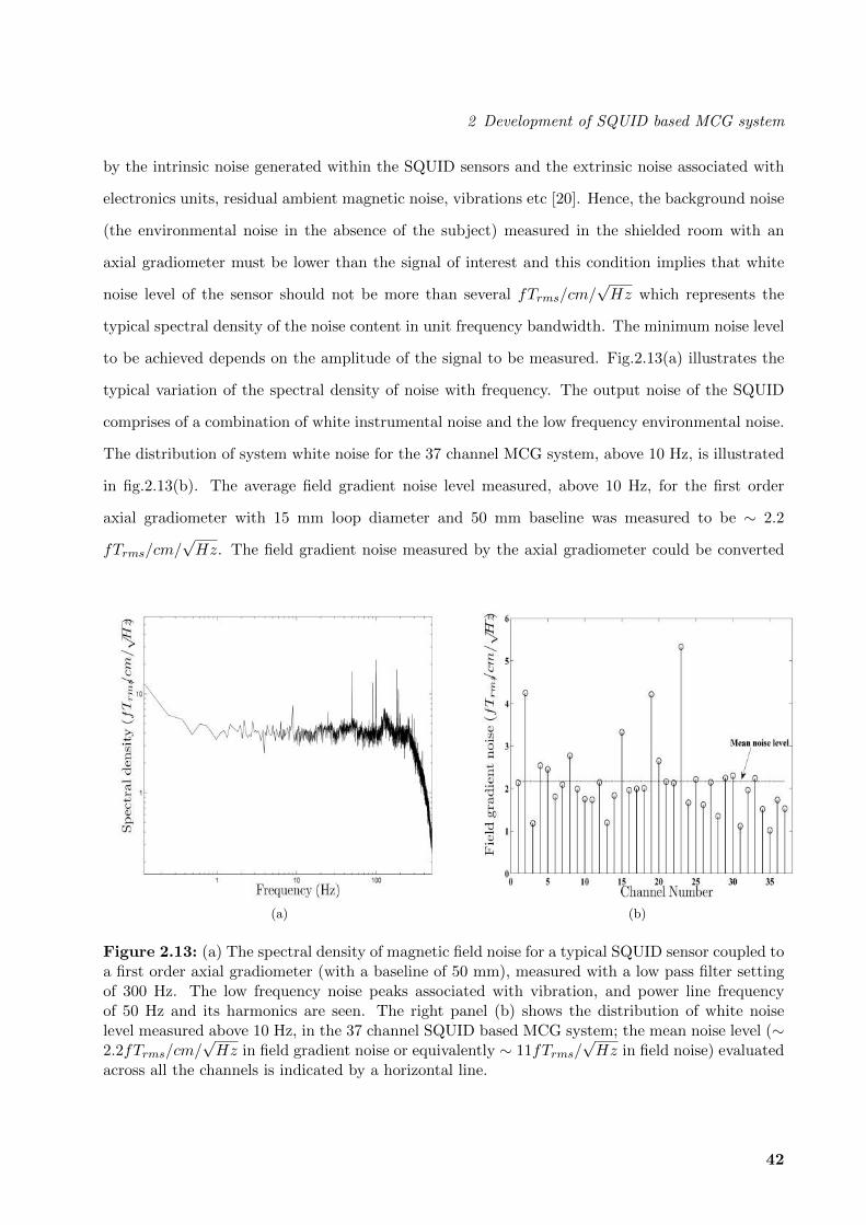
to be achieved depends on the amplitude of the signal to be measured. Fig.2.13(a) illustrates the
typical variation of the spectral density of noise with frequency. The output noise of the SQUID
comprises of a combination of white instrumental noise and the low frequency environmental noise.
The distribution of system white noise for the 37 channel MCG system, above 10 Hz, is illustrated
in fig.2.13(b). The average field gradient noise level measured, above 10 Hz, for the first order
axial gradiometer with 15 mm loop diameter and 50 mm baseline was measured to be ∼ 2.2
fTrms/cm/√Hz. The field gradient noise measured by the axial gradiometer could be converted
(a) (b)
Figure 2.13: (a) The spectral density of magnetic field noise for a typical SQUID sensor coupled toa first order axial gradiometer (with a baseline of 50 mm), measured with a low pass filter settingof 300 Hz. The low frequency noise peaks associated with vibration, and power line frequencyof 50 Hz and its harmonics are seen. The right panel (b) shows the distribution of white noiselevel measured above 10 Hz, in the 37 channel SQUID based MCG system; the mean noise level (∼2.2fTrms/cm/
√Hz in field gradient noise or equivalently ∼ 11fTrms/
√Hz in field noise) evaluated
across all the channels is indicated by a horizontal line.
42

2 Development of SQUID based MCG system
into an equivalent magnetic field noise by multiplying the field gradient noise by the baseline length
of the gradiometer [20]. The average magnetic field noise is thus inferred to be ∼ 11 fTrms/√Hz
for our MCG system.
2.7 MCG Measurement
Before MCG recording, the SQUID sensors are tuned to the correct bias current at which the
maximum modulation depth is observed, which usually corresponds to the minimum output noise
in the Flux Locked Loop (FLL) mode. The subject is instructed to remove and deposit all magnetic
and metallic objects (including currency notes, which are usually printed with a magnetic ink). The
subject is then taken inside the Magnetically Shielded Room (MSR), and is positioned under the
cryostat in a supine position by appropriately raising or lowering the cryostat along the vertical
axis. It is important to adjust the vertical position of the cryostat in such a way as to minimize
the distance between the sensor plane and the subject to realize a high signal-to-noise ratio during
the MCG measurements; nevertheless, care should be taken to ensure that the body of the subject
does not touch the cryostat and that there is a clear gap between them. After the position of the
subject under the cryostat is adjusted to align the central axis of the cryostat with reference to
selected anatomical reference points on the thorax of the subject, the pneumatic door of the MSR
is closed. The MCG signal is then recorded using the SQUID sensor array and is displayed on the
server PC of the data acquisition system located in the unshielded environment. For recording, we
typically use a sampling rate of 1 kHz in each channel with a low pass filter setting of 300 Hz and
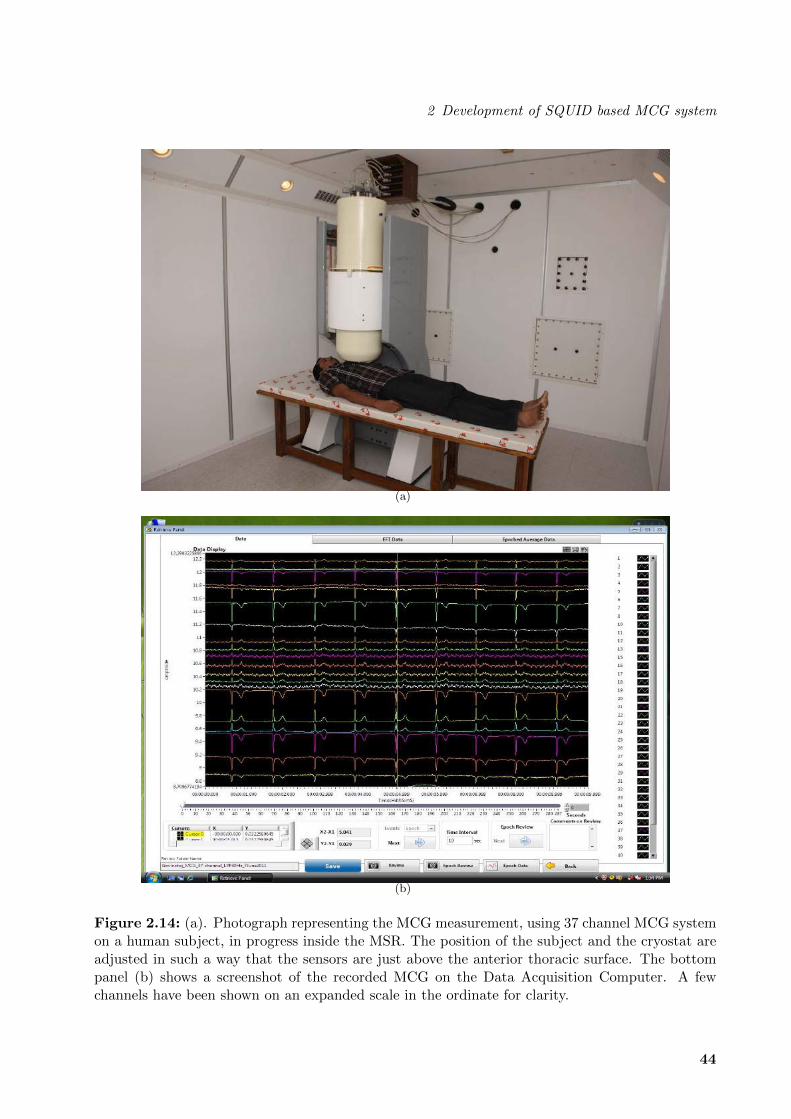
the FLL is usually operated at a gain setting of 5 V/Φ0. Fig.2.14(a) shows a photograph of the
MCG recording on a human subject in progress inside the MSR using the 37 channel MCG system;
fig.2.14(b) shows the recorded MCG on the Data Acquisition Computer.
43
2 Development of SQUID based MCG system
(a)
(b)
Figure 2.14: (a). Photograph representing the MCG measurement, using 37 channel MCG systemon a human subject, in progress inside the MSR. The position of the subject and the cryostat areadjusted in such a way that the sensors are just above the anterior thoracic surface. The bottompanel (b) shows a screenshot of the recorded MCG on the Data Acquisition Computer. A fewchannels have been shown on an expanded scale in the ordinate for clarity.
44
2 Development of SQUID based MCG system
2.8 MCG signal source analysis
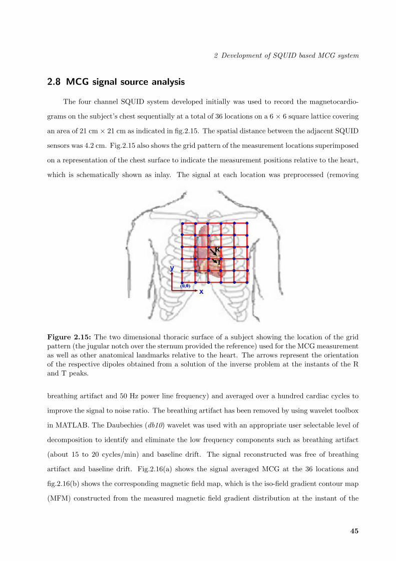
The four channel SQUID system developed initially was used to record the magnetocardio-
grams on the subject’s chest sequentially at a total of 36 locations on a 6 × 6 square lattice covering
an area of 21 cm × 21 cm as indicated in fig.2.15. The spatial distance between the adjacent SQUID
sensors was 4.2 cm. Fig.2.15 also shows the grid pattern of the measurement locations superimposed
on a representation of the chest surface to indicate the measurement positions relative to the heart,
which is schematically shown as inlay. The signal at each location was preprocessed (removing
Figure 2.15: The two dimensional thoracic surface of a subject showing the location of the gridpattern (the jugular notch over the sternum provided the reference) used for the MCG measurementas well as other anatomical landmarks relative to the heart. The arrows represent the orientationof the respective dipoles obtained from a solution of the inverse problem at the instants of the Rand T peaks.
breathing artifact and 50 Hz power line frequency) and averaged over a hundred cardiac cycles to
improve the signal to noise ratio. The breathing artifact has been removed by using wavelet toolbox
in MATLAB. The Daubechies (db10) wavelet was used with an appropriate user selectable level of
decomposition to identify and eliminate the low frequency components such as breathing artifact
(about 15 to 20 cycles/min) and baseline drift. The signal reconstructed was free of breathing
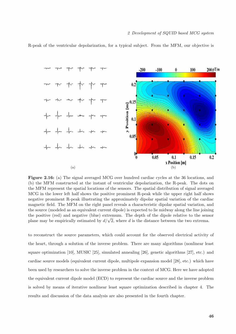
artifact and baseline drift. Fig.2.16(a) shows the signal averaged MCG at the 36 locations and
fig.2.16(b) shows the corresponding magnetic field map, which is the iso-field gradient contour map
(MFM) constructed from the measured magnetic field gradient distribution at the instant of the
45
2 Development of SQUID based MCG system
R-peak of the ventricular depolarization, for a typical subject. From the MFM, our objective is
(a) (b)
Figure 2.16: (a) The signal averaged MCG over hundred cardiac cycles at the 36 locations, and(b) the MFM constructed at the instant of ventricular depolarization, the R-peak. The dots onthe MFM represent the spatial locations of the sensors. The spatial distribution of signal averagedMCG in the lower left half shows the positive prominent R-peak while the upper right half showsnegative prominent R-peak illustrating the approximately dipolar spatial variation of the cardiacmagnetic field. The MFM on the right panel reveals a characteristic dipolar spatial variation, andthe source (modeled as an equivalent current dipole) is expected to lie midway along the line joiningthe positive (red) and negative (blue) extremum. The depth of the dipole relative to the sensorplane may be empirically estimated by d/
√2, where d is the distance between the two extrema.
to reconstruct the source parameters, which could account for the observed electrical activity of
the heart, through a solution of the inverse problem. There are many algorithms (nonlinear least
square optimization [10], MUSIC [25], simulated annealing [26], genetic algorithms [27], etc.) and
cardiac source models (equivalent current dipole, multipole expansion model [28], etc.) which have
been used by researchers to solve the inverse problem in the context of MCG. Here we have adopted
the equivalent current dipole model (ECD) to represent the cardiac source and the inverse problem
is solved by means of iterative nonlinear least square optimization described in chapter 4. The
results and discussion of the data analysis are also presented in the fourth chapter.
46
2 Development of SQUID based MCG system
As already noted, the use of a four channel system for experimental measurements imposes
limitations on the possible accuracies in the positioning of the sensors exactly at the nodal points
of the grid during the measurement of the MCG at each of the nine configurations. This problem
could be circumvented if simultaneous measurements were made using a system with a larger
number of channels and covering a larger area of the thorax. In view of this, subsequent studies
have been carried out with 37 channel MCG system and also the advanced signal pre-processing
methods such as ensemble empirical mode decomposition method (described in chapter 3) has been
adopted for denoising since the conventional denoising methods like filtering, averaging, wavelet
based denoising, etc. have some drawbacks which are discussed in the third chapter.
47

Bibliography
[1] K. Gireesan, C. Parasakthi, S. Sengottuvel, N. Mariyappa, Rajesh Patel, M.P.Janawadkar and
T.S. Radhakrishnan. Establishment of 13 channel SQUID based MEG system for Studies in
biomagnetism. Indian J. Cryogenics. 36 (2012) 169 - 172.
[2] C. Parasakthi, Rajesh Patel, S. Sengottuvel, N. Mariyappa, K. Gireesan, M.P. Janawadkar and
T.S. Radhakrishnan. Establishment of 37 channel SQUID system for magnetocardiography. AIP
Conf. Proc. 1447 (2012) 871 - 872.
[3] Y. Nakaya and H. Mori. Magnetocardiography. Clin. Phys. Physiol. Meas. 13 (1992) 191 - 229.
[4] A. Braginski and J. Clarke. “Introduction.” In: The SQUID Handbook - Fundamentals and
Technology of SQUIDs and SQUID Systems - Vol I. edited by J. Clarke and A.I. Braginski.
Weinheim: WILEY-VCH, 2004, pp. 1 - 25.
[5] R.L. Fagaly. Superconducting quantum interference device instruments and applications. Rev.
Sci. Instrum. 77 (2006) 101101; doi: 10.1063/1.2354545.
[6] M.P. Janawadkar, R. Baskaran, Rita Saha, K. Gireesan, R. Nagendran, L.S. Vaidhyanathan,
J. Jayapandian and T.S. Radhakrishnan. SQUIDs Highly sensitive magnetic sensors. Curr. Sci.
77 (1999) 759 - 769.
[7] V. Pizzella, S.D. Penna, C.D. Gratta and G.L. Romani. SQUID systems for biomagnetic imag-
ing. Supercond. Sci. Technol. 14 (2001) R79 - R114.
[8] G. Stroink, B. Hailer and P. Van Leeuwen. “Cardiomagnetism.” In: Magnetism in Medicine,
edited by W. Andra and H. Nowak. Weinheim: WILEY-VCH, 2006, pp. 164 - 209.
48
Bibliography
[9] D. Drung and M. Muck. “SQUID Electronics.” In: The SQUID Handbook - Fundamentals and
Technology of SQUIDs and SQUID Systems - Vol I. edited by J. Clarke and A.I. Braginski.
Weinheim: WILEY-VCH, 2004, pp. 127 - 170.
[10] M. Hamalainen, R. Hari, R.J. Ilmoniemi, J. Knuutila and O.V. Lounasmaa.
Magnetoencephalography-theory, instrumentation, and applications to noninvasive studies of
the working human brain. Rev. Mod. Phys. 65 (1993) 413 - 497.
[11] S. J. Williamson and L. Kaufman. Biomagnetism. J. Magnetism and Magnetic Materials. 22
(1981) 129 - 201.
[12] Z. G. Ozdemir, O.A. Cataltepe and U. Onbasli. “Some Contemporary and Prospective Appli-
cations of High Temperature Superconductors.” In: Applications of High-Tc Superconductivity,
edited by A.M. Luiz. InTech, ISBN 978-953-307-308-8, 2011, pp. 15 - 44.
[13] K. Sternickel and A.I. Braginski. Biomagnetism using SQUIDs: status and perspectives. Su-
percond. Sci. Technol. 19 (2006) S160 - S171.
[14] J. Vrba. SQUID gradiometers in real environments. NATO ASI Series. 329 (1996) 117 - 178.
[15] J. Vrba, G. Haid, S. Lee, B. Taylor, A.A. Fife, P. Kubik, J. McCubbin and M.B. Burbank.
Biomagnetometers for unshielded and well shielded environments. Clin. Phys. Physiol. Meas. 12
(1991) 81 - 86.
[16] J. Vrba and S.E. Robinson. Signal Processing in Magnetoencephalography. METHODS. 25
(2001) 249 - 271.
[17] W.A.M. Aarnink, P.J. Van Den Bosch, T.M. Roelofs, M. Verbiesen, H.J. Holland, H.J.M. ter
Brake and H. Rogalla. Active noise compensation for multichannel magnetocardiography in an
unshielded environment. IEEE Trans. Appl. Supercond. 5(2) (1995) 2470 - 2473.
[18] H. Matsuba. “Magnetic Shielding by HTc Superconductor.” In: Advances in Superconductivity
IV, edited by H. Hayakawa and N. Koshizuka. Japan: Springer, 1992, pp. 1055 - 1060 .
[19] M.P. Janawadkar, T.S. Radhakrishnan, K. Gireesan, C. Parasakthi, S. Sengottuvel, Rajesh
49
Bibliography
Patel, C.S. Sundar and Baldev Raj. SQUID - based measurement of biomagnetic fields. Curr.
Sci. 99(1) (2010) 36 - 45.
[20] C.P. Foley, M.N. Keene, H.J.M ter Brake and J. Vrba. “SQUID system issues.” In: The SQUID
Handbook - Fundamentals and Technology of SQUIDs and SQUID Systems - Vol I. edited by J.
Clarke and A.I. Braginski. Weinheim: WILEY-VCH, 2004, pp. 251 - 355.
[21] H. Koch and W. Haberkorn. Magnetic field mapping of cardiac electrophysiological function.
Phil. Trans. R. Soc. Lond. A. 359 (2001) 1287 - 1298.
[22] P.C. Ribeiro, S.J. Williamson and L. Kaufman. SQUID arrays for simultaneous magnetic
measurements: calibration and source localization performance. IEEE Trans. Biomed. Eng. 35(7)
551 - 560.
[23] N. Mariyappa, C. Parasakthi, S. Sengottuvel, Rajesh Patel, K. Gireesan, T.S. Radhakrishnan,
M.P. Janawadkar and C.S. Sundar. Improving noise performance of the SQUID in the presence
of high resistive leads. AIP Conf. Proc. 1447 (2012) 891 - 892.
[24] P.H. Ornelas, A.C. Bruno, C. Hall Barbosa, E. Andrade Lima and P. Costa Ribeiro. A survey
of calibration procedures for SQUID gradiometers. Supercond. Sci. Technol. 16 (2003) 427 - 431.
[25] J.C. Mosher, P.S. Lewis and R.M. Leahy. Multiple dipole modeling and localization from
spatio-temporal MEG data. IEEE Trans. Biomed. Eng. 39 (1992) 541 - 557.
[26] H. Haneishi, N. Ohyama, K. Sekihara and T. Honda. Multiple current dipole estimation using
simulated annealing. IEEE Trans. Biomed. Eng. 41 (1994) 1004 - 1009.
[27] K. Uutela, M. Hamalainen and R. Salmelin, Global optimization in the localization of neuro-
magnetic sources. IEEE Trans. Biomed. Eng. 45 (1998) 716 - 723.
[28] Wang Qian, Ma Ping, Lu Hong, Tang Xue-Zheng, Hua Ning and Tang Fa-Kuan. Inverse
computation for cardiac sources using single current dipole and current multipole models. Chinese
Phys. B 18 (2009) 5566 - 5574.
50