1st Block, TK Labs Lecture Notes

MECN2005 Mechanical Engineering Laboratory 1

T. Kim

Lab courses

- 1st semester:(1) Fluids 1: Calibration of flowmeters (Prof. Kim)(2) Fluids 2: Fluid friction in pipe flow (Dr. Law)(3) Mechanics 1: Compression tests (Prof. Polese)(4) Mechanics 2: Forces in plane trusses (Dr. Muthu)

- 2nd semester:(5) Thermodynamics: The pressure relationship for w ater-steam(6) Heat transfer: Conduction heat transfer in a so lid(7) Mechanics 3: Single degree of freedom (DOF) vib ration(8) Mechanics 4: Compound pendulum

Typical engineering problem solving procedure

- System observation

- Problem identification

- Problem description

- Approach (1) Analytical (mathematical)(2) Numerical (simulation)(3) Experimental

- Solution- Re-design

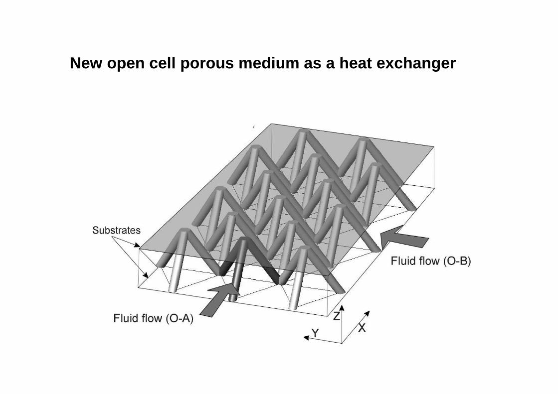
New open cell porous medium as a heat exchanger

(1) Analytical approach

- Mathematics based approach, providing details of the physical contribution of involved parameters.

- Validation needed since mathematical simplifications typically made during derivation.

ks [W/mK]

Nu dp

0 150 300 450 600 750 9000

100

200

300

400

500 from the estimation using the fin equation at Redp=20000from the estimation using the fin equation at Redp=5000from the experiments

Vertexpf

totaldp dk

qNu

Θ1

/=

+−=

yx

StrutsStrutVertexyxendwall

f

p

SS

mLAPkhASSh

k

d )tanh(3)(

Adopting a classical “fin” analogy,

(2) Numerical approach ( I )

- Mathematics based approach, BUT often some fitting constants (typically from empirical correlations) required.

- Once validated, providing deep physical insights into the problem.

(2) Numerical approach (II)

- Grid generation- Boundary conditions

Streamlines at selected surfaces with colored velocity magnitude

(3) Experimental approach (I)

- Physical observation of what actually is happening.

- Self-standing/validating solutions if well & accurately designed and conducted.

- Design of experiment is about what & how to measure. Unfortunately (?), already done by someone else.

- Performing experiment (by you)- Interpreting experimental data (by you)

(2) Experimental approach (II)

Small scale test rigwith channel height of 12 mm

Larger scale test rigwith channel height of 300 mm

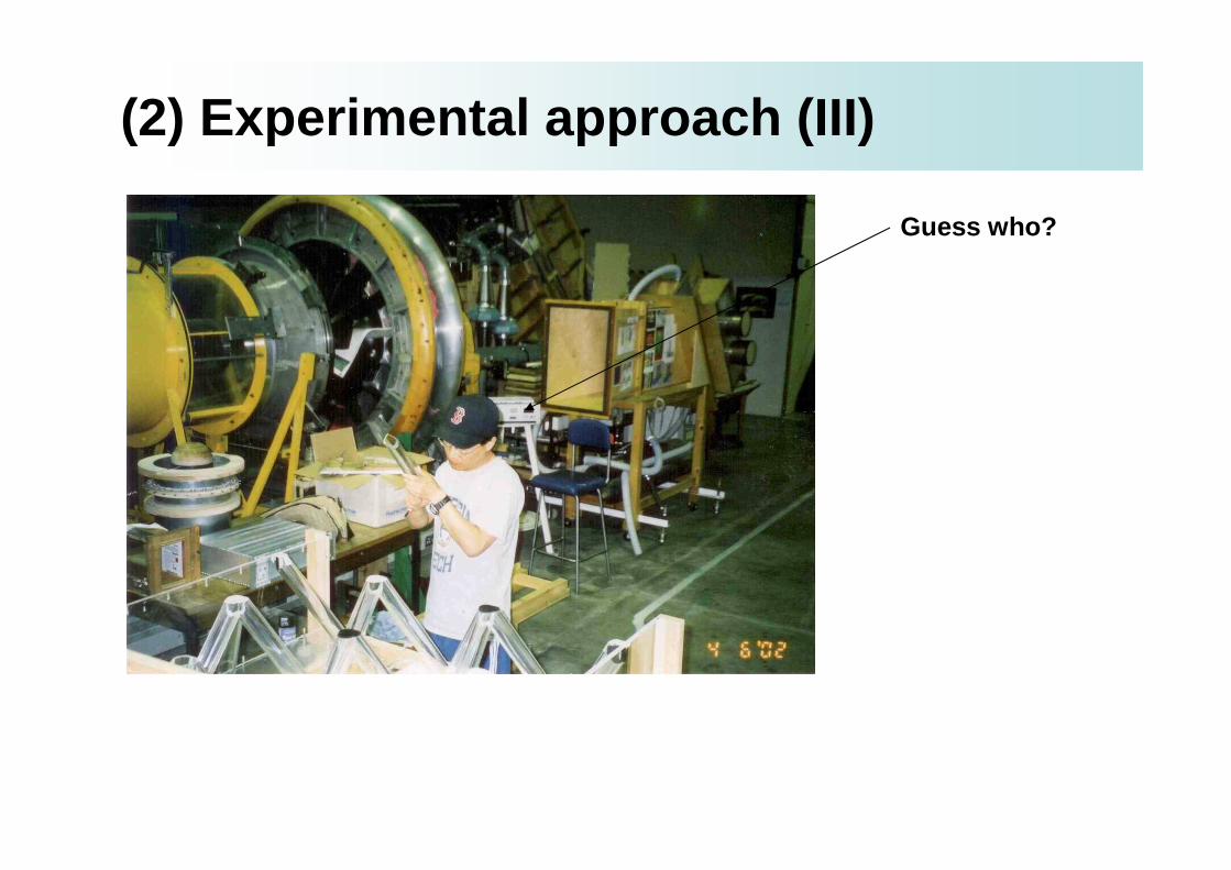
(2) Experimental approach (III)

Guess who?

Experimental

- Fluid Mechanics- Thermodynamics - Heat transfer- Mechanics

Fluid Mechanics: some related aspects

Experimental Thermo -Fluid Mechanics

Experiments? Dirty work???

Despite continuing advances in computational fluid dynamics (CFD), experimental data are still needed to “validate” the CFD results. Therefore, a sound knowled ge of experimentation is a necessary asset for not only experimentalists but also CFD people .

For any experiment, a fundamental question is perhaps “what to measure.” Answering this question is likely to be associated with governing equations . Three governing equations in aerodynamics and heat transfer include “ continuity equation ”, “ momentum equation ,” and “ energy equation .”These equations contain the terms such as (1) static pressure , (2) velocity , (3) temperature , and (4) their gradients .


The measurement techniques in this lecture attempt to quantify some of them in different media-gases, and liquids.

In some cases, it is not possible at present to experimentally obtain parameters required to close the above-mentioned governing equations due to the experimental limitations ( ???? ).

There are parameters in the governing equations that may not be experimentally quantified without compromising data quality as could be done analytically.

0=dx

duρ

2

2

dx

ud

dx

dp

dx

duu µρ +−=

The motion of fluid particles is governed by the Navier-Stokes(N-S) equation. In addition, the fluid has to satisfy t he “ continuity equation ” stating mass conservation for a given volume of interest (control volume). In one-dimensional form, al ong the x-axis, the general expressions of these equations for incompressible and steady flow without body force may be expressed as:

- Continuity equation:

- Momentum equation:

where u is the velocity component in the x-direction, p is the static pressure, ρρρρ is the density of fluid, and μμμμ is the viscosity of fluid.


Details of the final expression of both equations in cluding mathematical derivations can be readily found in nume rous text books.


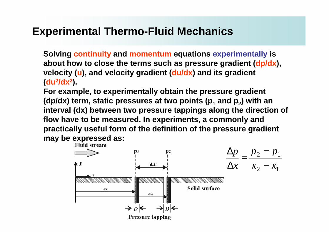
Solving continuity and momentum equations experimentally is about how to close the terms such as pressure gradient (dp /dx ), velocity ( u), and velocity gradient ( du /dx ) and its gradient (du 2/dx 2). For example, to experimentally obtain the pressure gra dient (dp /dx ) term, static pressures at two points ( p1 and p2) with an interval ( dx ) between two pressure tappings along the direction of flow have to be measured. In experiments, a commonly and practically useful form of the definition of the pres sure gradient may be expressed as:

12

12

xx

pp

x

p

−−

=∆∆


In the actual experimental setup, the closest interva l (∆∆∆∆x) might be the diameter of the pressure tappings, D, which is typically on the order of millimeters.

For detailed gradient measurements, if many pressure tappings are aligned along the x-axis with “very fine intervals” (e.g., ~ the diameter of the pressure tapping s), another unexpected problem may arise. The flow past th e downstream tappings will be affected by those at upstr eam because the upstream tappings may act as cavities an d alter the flow.

There m ay exist a minimum interval (between two pressure tappings placed in an in-lined configuration along th e x-axis) which minimizes such interference effects without s acrificing data resolution.


Similarly, the velocity gradient terms can be obtaine d by measuring velocity at different locations (separated by ∆∆∆∆x) using various techniques (e.g., Laser Doppler Anemometry (LDA), Pitot tube).

The accuracy of the measurements depends strongly on ∆∆∆∆x and its relative scale to the overall flow domain of interest and probe size. Thus, experimental data are strongly dependent upon measurement methods. Therefore, it is important to question whether an appropriate experimental technique that does not contaminate the main features of interest is being u sed.


Pipe flow and friction

[iraq-businessnews.com]

Exact solution (I)

The velocity at the wall is zero (i.e., non-slip con dition), because of adhesion, and reaches a maximum on the axis.

At a sufficiently large distance from the entrance sec tion the velocity distribution across the section becomes inde pendent of the coordinate along the direction of flow, called “? ???.”

The fluid moves under the influence of the pressure gradient which acts in the direction of the axis, whereas in s ections which are perpendicular to it the pressure may be constant.

Exact solution (II)

Owing to friction individual layers act on each other with a shearing stress which is proportional to the velocity gradient du/dy.

dy

du~τ

dy

duC=τor where C is a constant

A fluid particle is accelerated by the pressure gradi ent and retarded by the frictional shearing stress.

Exact solution (III)

Consider a coaxial fluid cylinder of length, l and radius y. The condition of equilibrium in the x-direction requires t hat the pressure force (p1-p2)ππππy2 acting on the faces of the cylinder be equal to the shear 2ππππylττττ acting on the circumferential area.

221 y

l

pp −=τ

Exact solution (III)

221 y

l

pp

dy

du

µ−−=

−−−=

4)(

221 y

Cl

ppyu

µ

( )2221

4)( yR

l

ppyu −−−=

µ

221

4R

l

ppum µ

−−=

( )21

42

82pp

l

RuRQ m −==

µππ

meanuRR

Q

Rl

pp222

21 88 µπ

µ =

=−

integrating

u=0 (no slip at the wall, y=R) �� C=R2/4

From the parabolic distribution of the velocity having the maximum u m at the center, y=0.

Volume flow rate

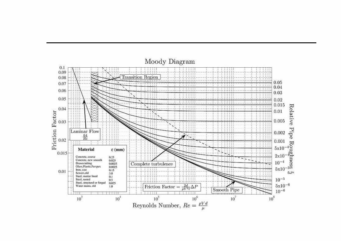
Measured pipe friction (I)

Friction factor

Reynolds number

2/221

meanu

d

l

ppf

ρ−=

µρ dumean

d =Re

duu

du

Ru

d

l

ppf

meanmeanmean

mean ρµ

ρµ

ρ64

2/

8

2/ 22221 =

=−=

Laminar friction loss in a pipe

d

fRe64=

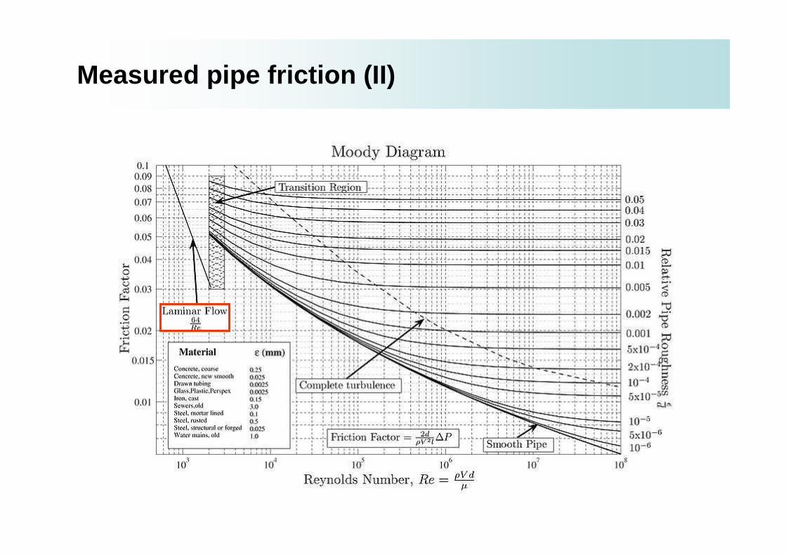
Measured pipe friction (II)

ReDh

Fric

tion

fact

or,f

2000 8000 14000 2000010-1

100

101

102

0 degree inclined15 degree inclined30 degree inclined45 degree inclined

Measured pipe friction (III)

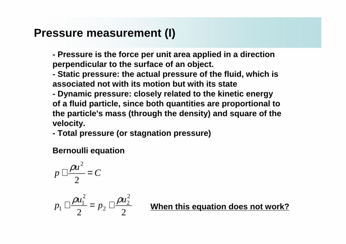
Pressure measurement (I)

- Pressure is the force per unit area applied in a direc tion perpendicular to the surface of an object. - Static pressure: the actual pressure of the fluid, wh ich is associated not with its motion but with its state - Dynamic pressure: closely related to the kinetic en ergy of a fluid particle, since both quantities are propor tional to the particle's mass (through the density) and square of the velocity. - Total pressure (or stagnation pressure)

Cu

p =+2

2ρ

Bernoulli equation

22

22

2

21

1u

pu

pρρ +=+ When this equation does not work?

Total pressure measurement

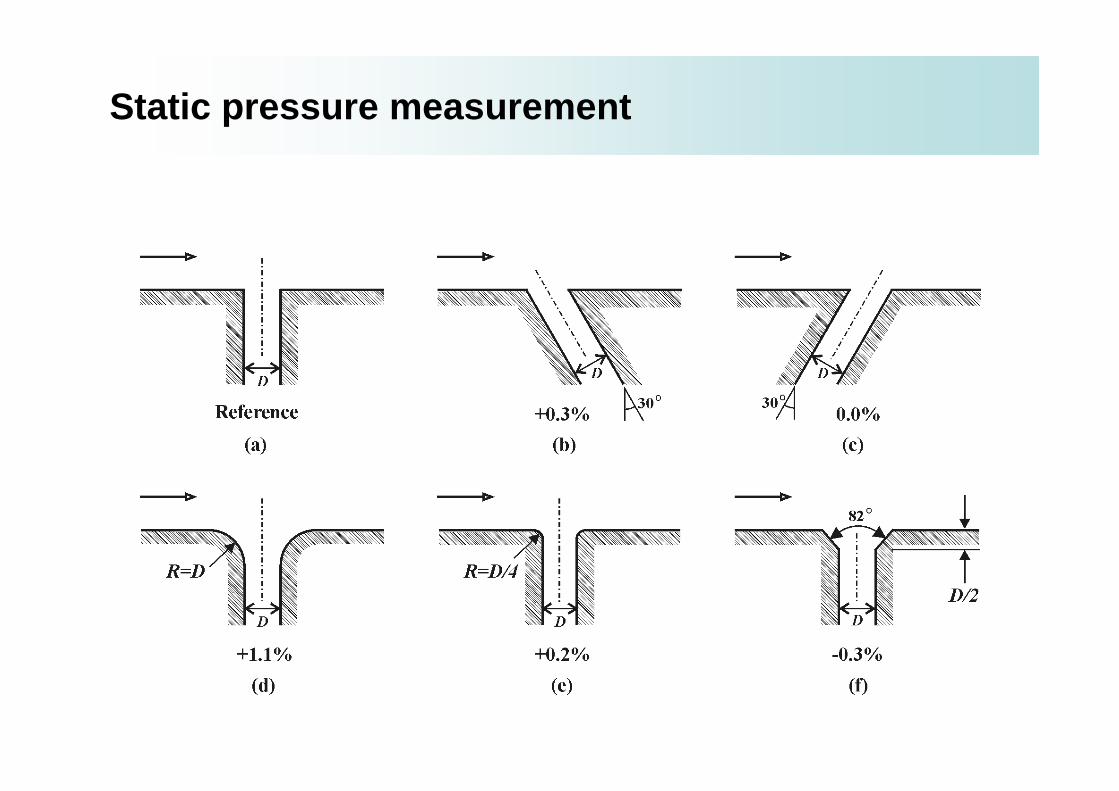
Static pressure measurement

Pressure drop vs. pressure loss

Empty channel (or pipe)

(p1 - p2)A (p1 - p2)B

Case A Case B

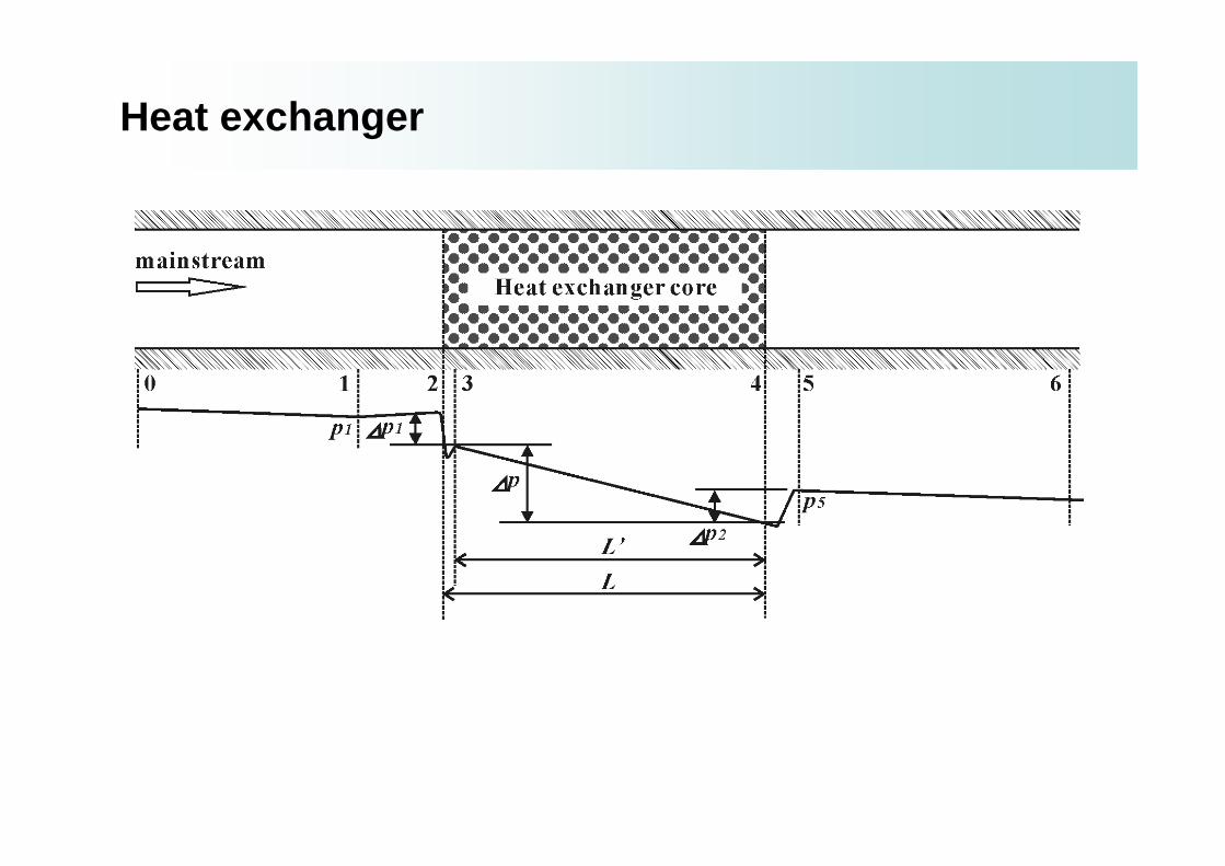
Heat exchanger

Mass & volume flow rate (I)

- Mechanical flow meters (e.g., Turbine flow meter, rotameter)- Pressure-based meters (e.g., Venturi nozzle, orifice plate)- Optical flow meters- Open channel flow measurement- Thermal mass flow meters- Vortex flowmeters- Electromagnetic, ultrasonic and coriolis flow meters- Laser Doppler flow measurement

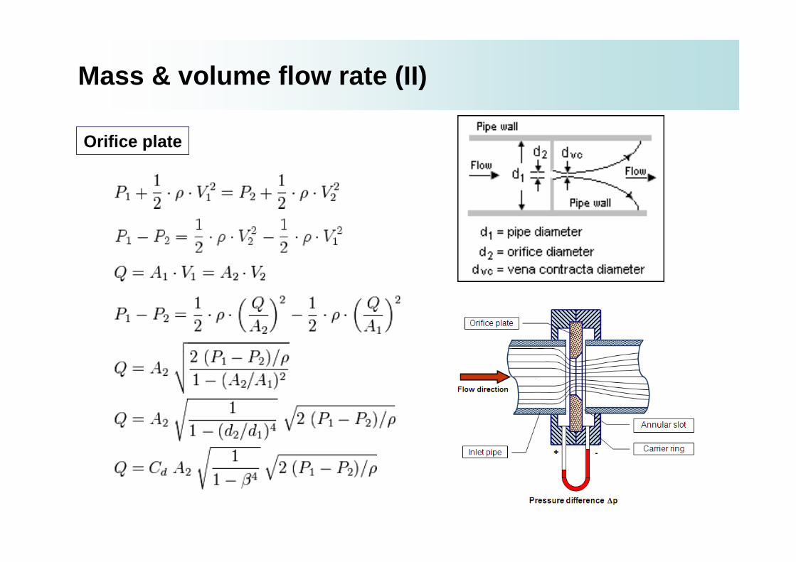
Orifice plate

Mass & volume flow rate (II)

Venturi nozzle http://en.wikipedia.org/wiki/Venturi_effect

Mass & volume flow rate (III)

Rotameter It belongs to a class of meters called variable area meters , which measure flow rate by allowing the cross-secti onal area the fluid travels through to vary, causing some mea surable effect.

A rotameter consists of a tapered tube, typically ma de of glass, with a float inside that is pushed up by flow and pulled down by gravity.

At a higher flow rate more area (between the float and the tube) is needed to accommodate the flow, so the float rises.

Readings are usually taken at the top of the widest part of the float; the center for an ellipsoid, or the t op for a cylinder.

Note that the "float" does not actually float in th e fluid: it has to have a higher density than the fluid, oth erwise it will float to the top even if there is no flow.

Mass & volume flow rate (IV)

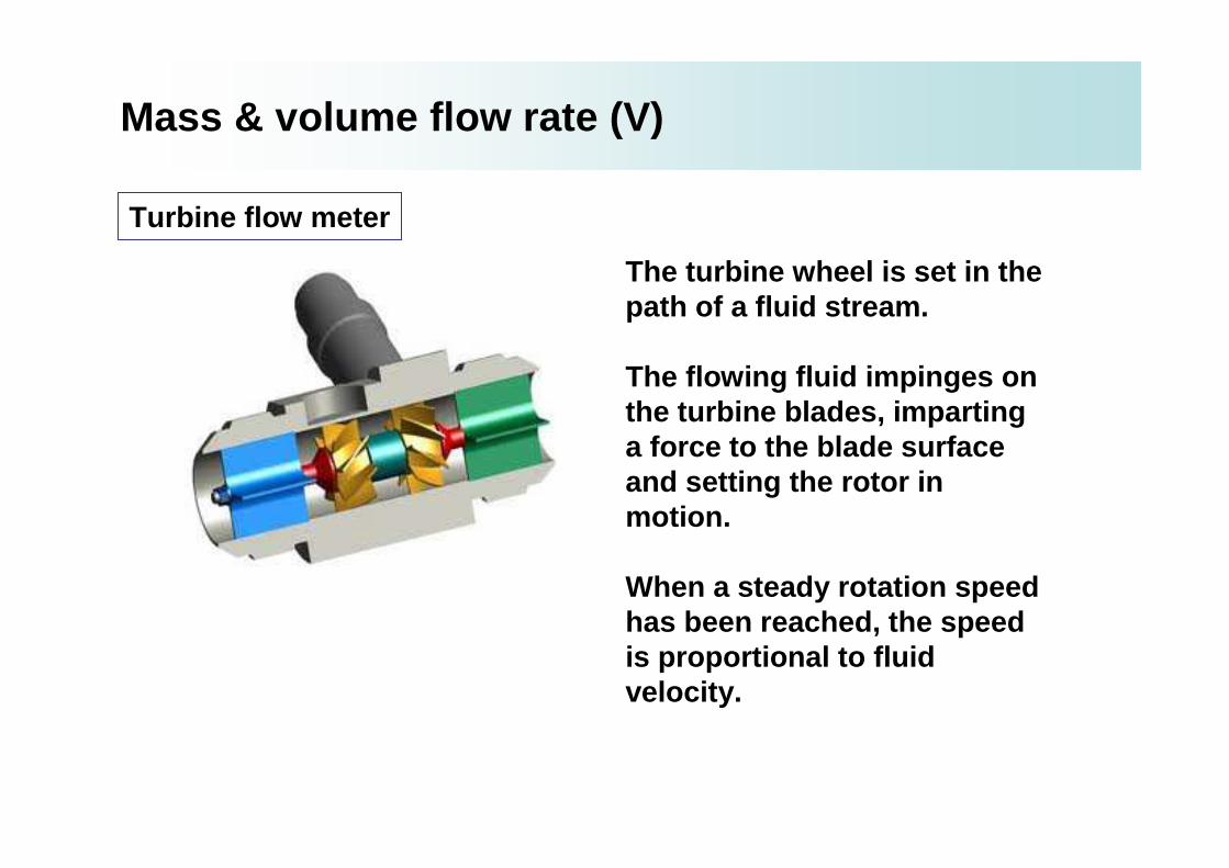
Turbine flow meter

Mass & volume flow rate (V)

The turbine wheel is set in the path of a fluid stream.

The flowing fluid impinges on the turbine blades, imparting a force to the blade surface and setting the rotor in motion.

When a steady rotation speed has been reached, the speed is proportional to fluid velocity.

Engineering Observation&

Physical Data Interpretation

Tongbeum Kim

Example case

www.treehugger.com

Simplified

Flow through a rectangular channel with many cylinders inserted forming a bank of cylinders.

(1) Cross-flow: design conditions(2) Off-design conditions

“Zero” degree inclined

Sideview

Problem considered: Inclination of Staggered Cylinder Banks

“Non-zero” degree inclined

Problem considered

- Frontal area is fixed,indicating that transverse pitch remains the same

- Porosity should be maintained,implying that longitudinal pitch varies with the in clination of the cylinders

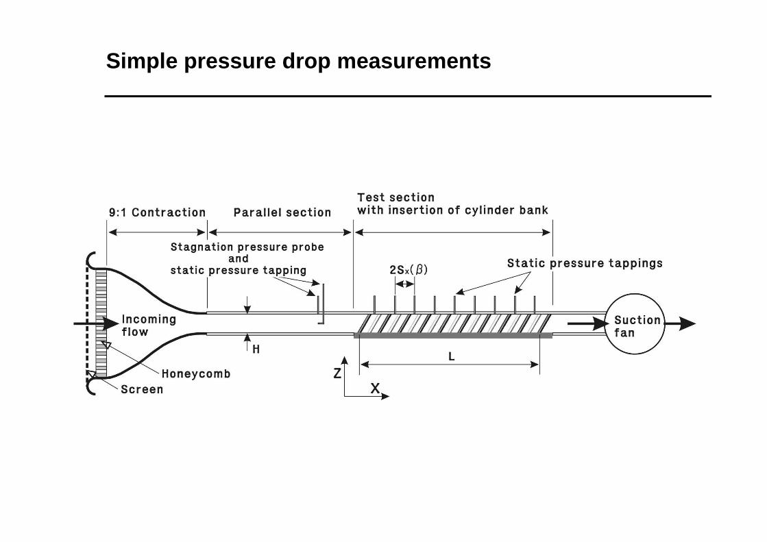
Simple pressure drop measurements

Data presentation

(1) Simple observation

U [m/s]

P/L

[pa/

m]

0 2 4 6 8 10 12 140

3000

6000

9000

12000

15000


∆

a. For a given inclination angle, dP/L v.s. U

b. What does classical (or conventional) equation say?

Following the same trend?

c. Any physical mechanism explained about its trend by other people?

d. Effect of the inclined angle in a qualitative manner?

In a quantitative manner?

Non-dimensional grouping

Why?????

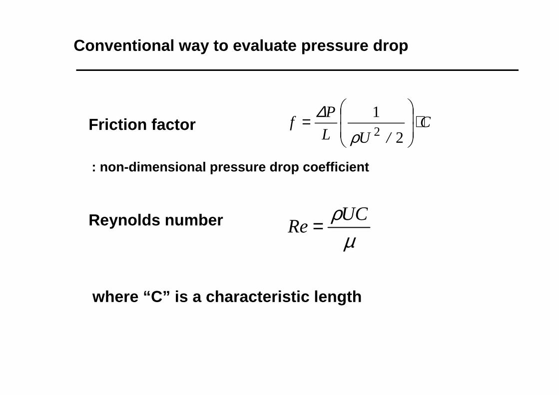
Conventional way to evaluate pressure drop

C/UL

Pf ⋅

=

2

12ρ

∆

µρUC

Re =

where “ C” is a characteristic length

Friction factor

Reynolds number

: non-dimensional pressure drop coefficient

- Cylinder diameter, d

- Circular pipe (flow channel) diameter, D

- Hydraulic diameter (for non-circular flow channel), D h

Dh=4(WH)/2(W+H) where W = Channel width

H = Channel height

Conventional choice of a characteristic length

ReDh

Fric

tion

fact

or,f

2000 8000 14000 2000010-1

100

101

102


Pressure drop across inclined staggered cylinder ba nks

Inclined angle

Pressure drop

What else?

New parameters using “ a variable unit cell length ”

- Pressure drop per unit cell, KCell

( ) ( )βρ

∆β xCell S/UL

PK

=

2

12

( )µ

βρ xdp

USRe =

- Reynolds number based on unit cell length

The beauty of non-dimensional grouping

ReSx( ),N

KC

ell,N

103 10410-1

100

101

102

0 degree inclined15 degree inclined30 degree inclined45 degree inclinedCorrelation

KCell,N = C / ReSx( ),N + Dβ

β

Variable unit cell length + Independence principle

DC

KNSx

NCell +=),(

, Re β

( ) )(cos)0(2)0(2

322

βρµβ∆

+

= U

SDU

SC

L

P

XX

where “ C” and “ D” are obtained from the non-inclined case.

1st Block, TK Labs Lecture Notes

Documents

Transcript of 1st Block, TK Labs Lecture Notes