Mathematical and Computer Modelling 49 (2009) 1078–1088

Contents lists available at ScienceDirect

Mathematical and Computer Modelling

journal homepage: www.elsevier.com/locate/mcm

1D gas dynamic modelling of mass conservation in engine duct systemswith thermal contact discontinuitiesJ.R. Serrano a,∗, F.J. Arnau a, P. Piqueras a, A. Onorati b, G. Montenegro b

a CMT - Motores Térmicos, Universidad Politécnica de Valencia, Spainb Dipartimento di Energia, Politecnico di Milano, Italy

a r t i c l e i n f o

Article history:Received 18 February 2008Accepted 27 March 2008

Keywords:Conservation equationsNumerical methodsThermal contact discontinuityMass conservationTime discretisation

a b s t r a c t

A detailed analysis of mass non-conservation in the proximity of thermal contactdiscontinuities, when solving 1-D gas dynamic flow equations with finite differencenumerical methods, is carried out in this paper. A wide spectrum of finite differencenumerical methods has been applied to solve such conditions. Thermal contactdiscontinuities are very common in current diesel engines due to back-flow in the intakevalves during the valve overlap period. Every method has been shown to be incapable ofcorrectly solving the problem raised, displaying (or revealing) a different behavior. Takingas base line these analyses a study regarding mesh size reduction in ducts has been alsoperformed. This solution becomes suitable since it leads to making mass conservationproblems disappear. Nevertheless, most extended calculation structure in 1D gas dynamicmodels is not advised due to the increase of computational effort required. Thus, a newcalculation structure for solving governing equations in ducts is suggested. This proposedcalculation structure is based on independent time discretisation of every duct accordingto its CFL stability criterion. Its application to thermal contact discontinuities points out itsadvantages with regard to computational demand as the calculation time of every duct isadapted to its mesh size.

© 2008 Elsevier Ltd. All rights reserved.

1. Introduction

Nowadays the challenging requirements of higher specific power, better fuel economy and increasingly stringentemission regulations [1] are demanding a significant effort from the automotive industry and researchers to develop a newgeneration of internal combustion engines. The optimization of gas flow through the engine intake and exhaust systems,involving the air filter and intake manifold, the EGR line, the turbocharger, the exhaust manifold, after-treatment andsilencing devices, is one of the key strategies in order to improve engine performance and to reduce pollutants emission.

In this field the use of thermo-fluid dynamic simulation models is producing unquestionable success due to its abilityto describe physical phenomena taking place in the engine. Thermo-fluid dynamic simulation models can be classified onthe basis of their complexity as mean value or quasi-steady models, filling and emptying models, one-dimensional (1-D)wave-action models and three dimensional calculation codes [2]. Among these computer codes, the development of one-dimensional (1-D) gas dynamic numerical models has become an essential tool to assist in the design [3] and developmentof new engines, as they can reproduce the effects on performance caused by modifications of the engine and its ductinggeometry. In recent years there has been a significant enhancement of one-dimensional gas dynamic numerical modelsand they have been widely used to simulate engine behaviour, from torque, power, fuel consumption [4,5] or exhaust gas

∗ Corresponding address: CMT - Motores Térmicos. PO Box 22012, E-46071, Valencia, Spain. Tel.: +34 963879657; fax: +34 963877659.E-mail address: jrserran@mot.upv.es (J.R. Serrano).

0895-7177/$ – see front matter © 2008 Elsevier Ltd. All rights reserved.doi:10.1016/j.mcm.2008.03.015

J.R. Serrano et al. / Mathematical and Computer Modelling 49 (2009) 1078–1088 1079

emissions [6,7] to noise emission prediction [8–10] or load transient evolution [11,12] and have shown a suitable balancebetween reliability, accuracy and calculation time [13,14].

One-dimensional gas dynamic models have to solve the 1-D unsteady non-homentropic mass, momentum and energyconservation laws. These governing equations form a non-homogeneous hyperbolic system. Nowadays, highly non-homentropic flow conditions can only be solved by means of numerical methods, despite the contribution of some workswith regard to the analytical solution of the governing equations system [15–17].

In most numerical models, the traditional mesh-method of characteristics (MOC) has been applied up to the mid1980’s [18]. Although the MOC is still widely used in the resolution of boundary conditions, owing to the comprehensiveand well-documented work existing on the treatment of every kind of flow boundary regions by means of a MOC-basedquasi-steady approach [19], in last decades the new generation of 1-D fluid dynamic models has adopted symmetric orupwind shock-capturing numerical methods in order to solve the hyperbolic problem of conservation equations. The originof these two important families of schemes was numerical techniques for resolution of the hyperbolic conservation lawssystem developed in the form of first-order methods by Courant et al. [20] and Lax [21]. On one hand, symmetric schemesapply a discretisation which is independent from inviscid flow characteristics. On the other hand, upwind schemes applydirectional space discretisations according to the physical behaviour of inviscid flows.

The second-order symmetric scheme proposed by Lax & Wendroff [22] is one of the most representative symmetricschemes. The main disadvantage of this method is the Jacobian matrix evaluation. To prevent the calculation from thisdifficulty, Richtmyer and Morton [23] suggested a two-step variant of the Lax & Wendroff method, leading to a whole familyof variants when applied to non-linear systems, represented by the MacCormack method [24].

A subgroup of upwind schemes is based on Godunov’s method [25] to solve, over each mesh interval, the local 1-DEuler equations for discontinuous neighbouring states. The second subgroup of upwind schemes is the flux vector splittingmethods, proposed by Steger and Warming [26].

Finite difference schemes, with greater than first-order accuracy and constant coefficients produce local instabilities inthe presence of shock waves and contact surfaces as a consequence of Godunov’s theorem [25]. These oscillations are non-physical and are known as Gibb’s phenomenon. To prevent from their generation, Boris and Book [27,28] developed the flux-corrected transport technique (FCT), whose three different steps to be solved were described by Niessner and Bulaty [29].These techniques represent the origin of high-resolution schemes.

Harten [30] developed the total variation diminishing (TVD) concept, whereby the variation of the numerical solution iscontrolled in a non-linear way, so as to avoid any new extremum from appearing.

Finally, Chang [31,32] introduced a new Euler solver named the conservation element-solution element method (CE–SE),based on a different approach with regard to the resolution of fundamental conservation equations. The peculiarity of thisscheme is that it does not employ any characteristic-based or flux-limiter method, but rather follows a simple approach togenerate highly accurate oscillation-free solutions.

Some authors have focused their efforts on adapting some of the previously developed schemes to solve non-homogeneous problems. In that way, Briz and Giannattasio [33] suggested a CE–SE method adaptation to solve thefundamental conservation equations system considering source terms. Later, Corberán and Gascón [34–36] simplified non-homentropic conservation equations in a homogeneous system by means of considering the source terms as part of the flowterms. Besides, the duct cross-sectional area was included in the conservation variables. The Lax & Wendroff method, theHarten TVD scheme and the flux-limiting techniques of Sweby were adapted according to this new approach [34–36]. Asimilar approach was carried out by Liu et al. [37] so as to propose the use of flux-corrected techniques in a conservativeway. Finally, Vandevoorde et al. [38] proposed a new cell-vertex TVD scheme to solve non-homoentropic conservation lawsbased on flux vector splitting techniques.

At the same time these approaches were being developed, the introduction of finite difference numerical methods in gasdynamic models [8,39–41] requires a continuous study of their behaviour under different flow conditions [42–45], in orderto optimise the choice of every method to be used in each case.

The work reported in the present paper carries on the studies regarding the effects of numerical methods on the solutionprovided and faces the analysis of the behaviour of numerical methods in the proximity of thermal contact discontinuities.Such a discontinuity represents an interface of two flows of gases with different composition and/or different temperature.The unsteady, compressible gas flow in the intake and exhaust systems of internal combustion engines includes regionswith varying composition and temperature. Especially critical is the thermal contact discontinuity produced in intake pipes,where this variation is mainly due to the back-flow of exhaust gas during valve overlap at low engine speed conditionsthat goes back again into the cylinders after a short time period. This study is developed from mass conservation problemsappearing in the proximity of thermal contact discontinuities taking place close to intake valves.

The work has been carried out by means of two 1-D gas dynamic models, WAM, from the Institute “CMT-MotoresTérmicos”, Universidad Politécnica de Valencia, and GASDYN, from Dipartimento di Energia, Politecnico di Milano. As a firststep, the authors have checked by means of both WAM and GASDYN the behaviour of several finite difference schemes inorder to describe them and attempt to clarify the possible causes of detected mass conservation problems in the proximityof thermal contact discontinuities. Then, this analysis has been extended to evaluate the influence of spatial mesh sizereduction on this concrete mass conservation problem. The improvement of the results concerning mass conservationcontrasts with the increase in computational effort, which would preclude the spatial mesh size reduction from beingadopted as a feasible solution to the related mass conservation problem. In order to minimise the effects of spatial mesh size

1080 J.R. Serrano et al. / Mathematical and Computer Modelling 49 (2009) 1078–1088

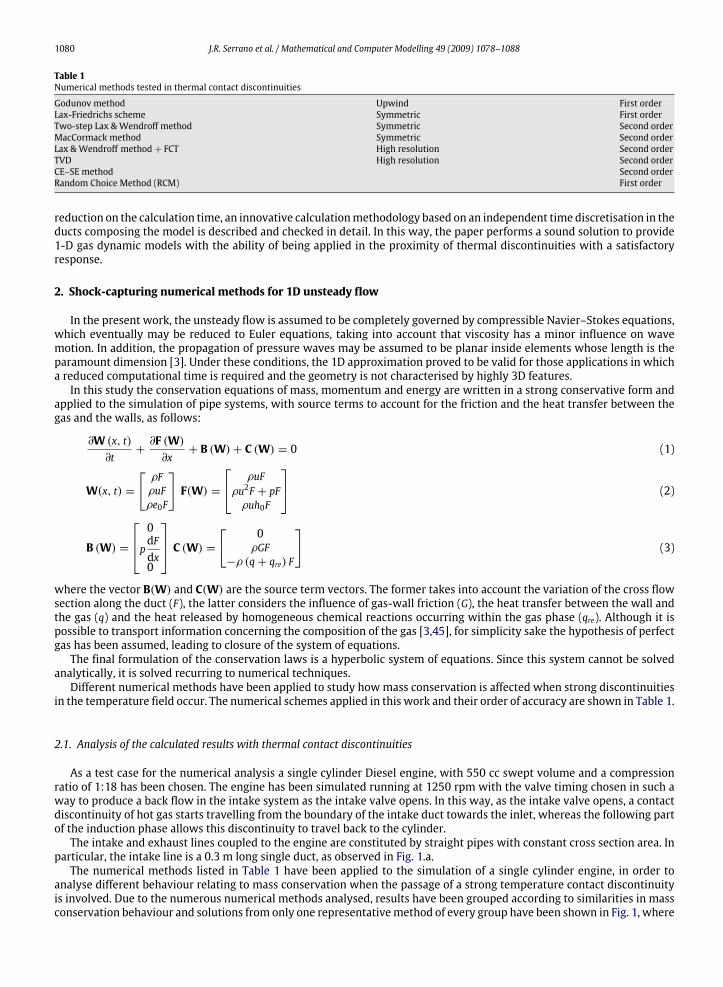
Table 1Numerical methods tested in thermal contact discontinuities

Godunov method Upwind First orderLax-Friedrichs scheme Symmetric First orderTwo-step Lax & Wendroff method Symmetric Second orderMacCormack method Symmetric Second orderLax & Wendroff method+ FCT High resolution Second orderTVD High resolution Second orderCE–SE method Second orderRandom Choice Method (RCM) First order

reduction on the calculation time, an innovative calculation methodology based on an independent time discretisation in theducts composing the model is described and checked in detail. In this way, the paper performs a sound solution to provide1-D gas dynamic models with the ability of being applied in the proximity of thermal discontinuities with a satisfactoryresponse.

2. Shock-capturing numerical methods for 1D unsteady flow

In the present work, the unsteady flow is assumed to be completely governed by compressible Navier–Stokes equations,which eventually may be reduced to Euler equations, taking into account that viscosity has a minor influence on wavemotion. In addition, the propagation of pressure waves may be assumed to be planar inside elements whose length is theparamount dimension [3]. Under these conditions, the 1D approximation proved to be valid for those applications in whicha reduced computational time is required and the geometry is not characterised by highly 3D features.

In this study the conservation equations of mass, momentum and energy are written in a strong conservative form andapplied to the simulation of pipe systems, with source terms to account for the friction and the heat transfer between thegas and the walls, as follows:

∂W (x, t)

∂t+∂F (W)

∂x+ B (W)+ C (W) = 0 (1)

W(x, t) =

ρFρuFρe0F

F(W) =

ρuFρu2F + pFρuh0F

(2)

B (W) =

0

pdFdx0

C (W) =

0ρGF

−ρ (q+ qre) F

(3)

where the vector B(W) and C(W) are the source term vectors. The former takes into account the variation of the cross flowsection along the duct (F), the latter considers the influence of gas-wall friction (G), the heat transfer between the wall andthe gas (q) and the heat released by homogeneous chemical reactions occurring within the gas phase (qre). Although it ispossible to transport information concerning the composition of the gas [3,45], for simplicity sake the hypothesis of perfectgas has been assumed, leading to closure of the system of equations.

The final formulation of the conservation laws is a hyperbolic system of equations. Since this system cannot be solvedanalytically, it is solved recurring to numerical techniques.

Different numerical methods have been applied to study how mass conservation is affected when strong discontinuitiesin the temperature field occur. The numerical schemes applied in this work and their order of accuracy are shown in Table 1.

2.1. Analysis of the calculated results with thermal contact discontinuities

As a test case for the numerical analysis a single cylinder Diesel engine, with 550 cc swept volume and a compressionratio of 1:18 has been chosen. The engine has been simulated running at 1250 rpm with the valve timing chosen in such away to produce a back flow in the intake system as the intake valve opens. In this way, as the intake valve opens, a contactdiscontinuity of hot gas starts travelling from the boundary of the intake duct towards the inlet, whereas the following partof the induction phase allows this discontinuity to travel back to the cylinder.

The intake and exhaust lines coupled to the engine are constituted by straight pipes with constant cross section area. Inparticular, the intake line is a 0.3 m long single duct, as observed in Fig. 1.a.

The numerical methods listed in Table 1 have been applied to the simulation of a single cylinder engine, in order toanalyse different behaviour relating to mass conservation when the passage of a strong temperature contact discontinuityis involved. Due to the numerous numerical methods analysed, results have been grouped according to similarities in massconservation behaviour and solutions from only one representative method of every group have been shown in Fig. 1, where

J.R. Serrano et al. / Mathematical and Computer Modelling 49 (2009) 1078–1088 1081

Fig. 1. Temperature results of different numerical methods close to the intake valve with back-flow.

instantaneous temperature profiles are depicted. After the opening of the intake valve at 340 crank angle degrees, a back-flow brings hot gas from the combustion chamber into the intake pipe. This process is characterised by the presence of astrong discontinuity in the temperature field, which can be clearly seen in the temperature profile. During the following partof the induction phase the flow goes from the pipe to the cylinder, and the discontinuity is transported back to the cylinder.Since both the duration and the intensity of the back-flow are limited, the contact surface does not travel further than a fewcalculation nodes of the intake pipe.

In particular, methods with second-order accuracy symmetric schemes, such as the Lax & Wendroff method and theMacCormack method, are affected by numerical instabilities. An example of this aspect is the low gas temperature value,below 0 ◦C calculated at 2 and 6 cm from the intake valve, as it is depicted in Fig. 1.c.

The application of first order upwind methods, namely Godunov’s method, or the adoption of high resolution schemessuch as TVD or FCT schemes, allows a better behaviour in terms of instabilities, balanced, however, by the addition of a first-order component which contributes to excessive diffusion. In particular, the adoption of these numerical schemes preventsthe solution from being unbounded, but slightly smears the temperature discontinuity, as it can be observed in Fig. 1 Graphsb and d.

By contrast, the Random Choice Method, which is shown in Fig. 1.e, shows a particular behaviour. The solution is notaffected by the presence of numerical diffusivity at all. As a matter of fact, the randomly chosen solution state allows tocapture sharp gradients in the conserved fields with high resolution, exhibiting, however, a mismatch in the discontinuityposition. This mismatch is contained within half of the mesh and is proportional to mesh size.

1082 J.R. Serrano et al. / Mathematical and Computer Modelling 49 (2009) 1078–1088

2.2. Effect of the spatial mesh size reduction on mass conservation

The impact of thermal discontinuity on mass conservation changes with the numerical scheme applied in the simulation.In order to check the ability of every finite difference numerical method to deal with this phenomenon a study of the spatialmesh size of the intake duct has been performed. Four spatial mesh sizes have been considered in this study, 5, 10, 20 and50 mm. The results are shown in Fig. 2, where the mass conservation error calculated at every node, according to Eq. (4),has been plotted.

MassConservationErrori(%) =

mi1tcycle

−

n∑j

mj1tcycle

nn∑j

mj1tcycle

n

(4)

where• n is the total number of nodes;• mi represents the mass of air that goes through the node i;• tcycle is the cycle duration.

Whichever finite difference numerical method has been applied, noteworthy conservation mass problems have beenproved close to the intake valve if a high temperature back-flow takes place, which is a common phenomenon in internalcombustion engines. Nevertheless, Fig. 2 shows clearly how the mass conservation error is reduced as the mesh size isreduced for every method tested. Furthermore, the behaviour of every numerical method can be classified into first-orderupwind scheme behaviour such as Godunov’s method, into second-order symmetric scheme behaviour, such as the two-step Lax & Wendroff method and the MacCormack method, or into high resolution scheme behaviour, such as TVD and thetwo-step Lax & Wendroff method+ FCT. Although the CE–SE method cannot be classified as a high resolution scheme, dueto its behaviour relating mass conservation close to thermal discontinuities it can be fallen into this group, as observed inFig. 2. The Random Choice Method and Lax–Friedrichs scheme have shown their own particular behaviour respectively.

The numerical instability of second-order symmetric schemes is also confirmed by the trend of the mass conservationerror (Fig. 2 Graphs c and d), which oscillates around an average value decreasing its amplitude with the distance from thevalve. However, second-order symmetric schemes provide better results, since to obtain a mass conservation error less than1% along the duct the spatial mesh size can be fixed to 20 mm. Under these conditions, reducing the spatial mesh size to10 mm results in a very accurate calculation, as shown in Fig. 2. Nevertheless, oscillation of the mean air mass flow along thenodes can be critical in order to carry out the transport of chemical species calculations, since it could lead to non-physicalsolutions.

Although first order upwind and high-resolution methods contribute to make instabilities disappear, they do notguarantee a completely bounded solution, also resulting in a distortion of the solution. This aspect is evident in Fig. 2 Graphsa, e, f and g, where the mass conservation error, which is remarkable in correspondence of the intake valve, decreases withthe distance from the valve and becomes asymptotic with slight oscillations around a positive value. The Random ChoiceMethod also shows a similar behaviour, although due to the absence of numerical diffusivity, its mass conservation errorresults in a flat profile along the intake duct, with the only exception being the first node, in which typical randomness of thesolution can be spotted. Regarding spatial mesh size, for these types of numerical methods it needs higher reduction, at leastup to 10 mm. The Lax-Friedrichs scheme tends to introduce too much numerical diffusion, hence it excessively propagatesthe error, which is characterised by the highest maximum value and is hardly affected by spatial mesh size reduction.

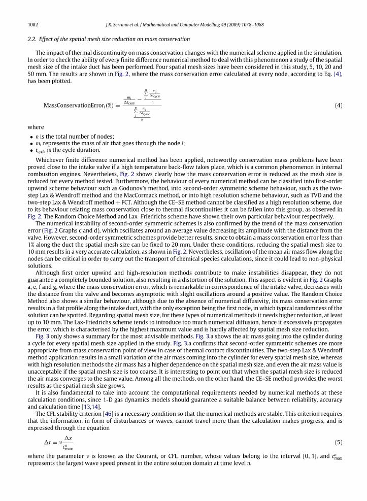
Fig. 3 only shows a summary for the most advisable methods. Fig. 3.a shows the air mass going into the cylinder duringa cycle for every spatial mesh size applied in the study. Fig. 3.a confirms that second-order symmetric schemes are moreappropriate from mass conservation point of view in case of thermal contact discontinuities. The two-step Lax & Wendroffmethod application results in a small variation of the air mass coming into the cylinder for every spatial mesh size, whereaswith high resolution methods the air mass has a higher dependence on the spatial mesh size, and even the air mass value isunacceptable if the spatial mesh size is too coarse. It is interesting to point out that when the spatial mesh size is reducedthe air mass converges to the same value. Among all the methods, on the other hand, the CE–SE method provides the worstresults as the spatial mesh size grows.

It is also fundamental to take into account the computational requirements needed by numerical methods at thesecalculation conditions, since 1-D gas dynamics models should guarantee a suitable balance between reliability, accuracyand calculation time [13,14].

The CFL stability criterion [46] is a necessary condition so that the numerical methods are stable. This criterion requiresthat the information, in form of disturbances or waves, cannot travel more than the calculation makes progress, and isexpressed through the equation

1t = ν1x

cnmax(5)

where the parameter ν is known as the Courant, or CFL, number, whose values belong to the interval [0, 1], and cnmaxrepresents the largest wave speed present in the entire solution domain at time level n.

J.R. Serrano et al. / Mathematical and Computer Modelling 49 (2009) 1078–1088 1083

Fig. 2. Analysis of mass conservation error in the intake duct for every mesh configuration and numerical method tested.

In some numerical methods this condition is more restrictive [47]. In that way, when the mesh spatial size is reduced, thetime step has to be diminished proportionally. Therefore, the computational effort significantly increases with the spatialmesh size reduction.

1084 J.R. Serrano et al. / Mathematical and Computer Modelling 49 (2009) 1078–1088

Fig. 3. Performance of numerical methods with respect to: (a) Air mass calculation through the intake valve; (b) Computational requirements of everymesh configuration and numerical method.

Generally 1-D gas dynamic codes calculate every engine component, namely ducts, plenums, cylinders, etc, with acommon time-step. Hence, to ensure the stability for each modelled duct, the time step must be in accordance with themost restrictive of all the ducts. Fig. 3.b shows a comparison of computational requirements needed by different numericalmethods at each spatial mesh size configuration. The average values of computational duration have been representedreferring to the two-step Lax & Wendroff method computational effort using the spatial mesh size of 50 mm.

Fig. 3.b points out that high-resolution schemes are the most affected by the spatial mesh size reduction, being the TVDmethod the most damaged when the spatial mesh size is severely reduced, owing to the fact that this scheme is based onthe Jacobian matrix resolution.

It is convenient to underline that the two-step Lax & Wendroff method with a spatial mesh size of 20 mm achieves a massconservation error less than 1% and its computational time just slightly grows regarding 50 mm configuration. However,high-resolution schemes need to apply a spatial mesh size of 10 mm, or smaller for the specific case of the CE–SE method,to approximately reach the 1% error level. This behaviour leads to nearly double the computational time required by highresolution schemes to achieve the same accuracy than the two-step Lax & Wendroff method in the case of a 20 mm mesh size,and evidences that the two-step Lax & Wendroff method application is more advisable for mass conservation against thermalcontact discontinuities resolution, although it is needed to take into account its problems with regard to temperature andmass oscillation along the nodes.

3. Calculation methodology approach based on independent time discretisation

It is clear that to reduce the spatial mesh size in a specific duct (in this case the intake duct) leads to an increase in thenumber of calculations per real time unit of every engine component. This fact gives rise to very high run-times to calculate acertain number of engine cycles. Nowadays it is common to adopt 1D codes for the simulation of engine transients. Therefore,since the number of cycles to be simulated is usually very large, an arbitrary mesh size reduction is not an advisable solution.

A possible solution may consist in using an independent time discretisation in ducts to be applied in 1-D gas dynamicsmodels. This new calculation approach allows spatial mesh size reduction in specific ducts without noticeably damagingglobal calculation time and achieving great accuracy.

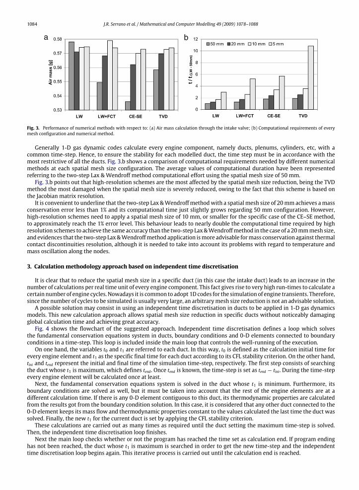
Fig. 4 shows the flowchart of the suggested approach. Independent time discretisation defines a loop which solvesthe fundamental conservation equations system in ducts, boundary conditions and 0-D elements connected to boundaryconditions in a time-step. This loop is included inside the main loop that controls the well-running of the execution.

On one hand, the variables t0 and t1 are referred to each duct. In this way, t0 is defined as the calculation initial time forevery engine element and t1 as the specific final time for each duct according to its CFL stability criterion. On the other hand,tini and tend represent the initial and final time of the simulation time-step, respectively. The first step consists of searchingthe duct whose t1 is maximum, which defines tend. Once tend is known, the time-step is set as tend − tini. During the time-stepevery engine element will be calculated once at least.

Next, the fundamental conservation equations system is solved in the duct whose t1 is minimum. Furthermore, itsboundary conditions are solved as well, but it must be taken into account that the rest of the engine elements are at adifferent calculation time. If there is any 0-D element contiguous to this duct, its thermodynamic properties are calculatedfrom the results got from the boundary condition solution. In this case, it is considered that any other duct connected to the0-D element keeps its mass flow and thermodynamic properties constant to the values calculated the last time the duct wassolved. Finally, the new t1 for the current duct is set by applying the CFL stability criterion.

These calculations are carried out as many times as required until the duct setting the maximum time-step is solved.Then, the independent time discretisation loop finishes.

Next the main loop checks whether or not the program has reached the time set as calculation end. If program endinghas not been reached, the duct whose t1 is maximum is searched in order to get the new time-step and the independenttime discretisation loop begins again. This iterative process is carried out until the calculation end is reached.

J.R. Serrano et al. / Mathematical and Computer Modelling 49 (2009) 1078–1088 1085

Fig. 4. Flowchart of independent time discretisation program layout.

The MOC method has been applied for the resolution of boundary conditions from the characteristics Riemann variables,λ and β, and the entropy level [19]. The use of a calculation structure based on an independent time discretisation for eachduct requires adaptation of the boundary conditions resolution. On this matter, two kinds of boundary conditions have tobe distinguished, depending on the engine elements that the boundary condition connects.

The boundary condition between a duct discharging flow to a plenum, cylinder or any other 0-D engine element is solvedfrom the characteristic lines, λ and β, and the entropy level, and the output and input mass flows. There is no difference inthe way the boundary condition is solved with regard to the original programme layout. However, there is a difference lyingin the calculations carried out to get the thermodynamic properties in the 0-D element. Every time a contiguous duct issolved, the 0-D element has to be updated to the current time. In order to carry out the energy and mass balances in the0-D element, every pipe end connected to the 0-D element has to be considered. This fact leads to take into account thelast calculated results for every boundary condition, assuming the information is frozen since the last time they all werecalculated until the current time, that is set by the last calculated boundary condition connected to the 0-D element.

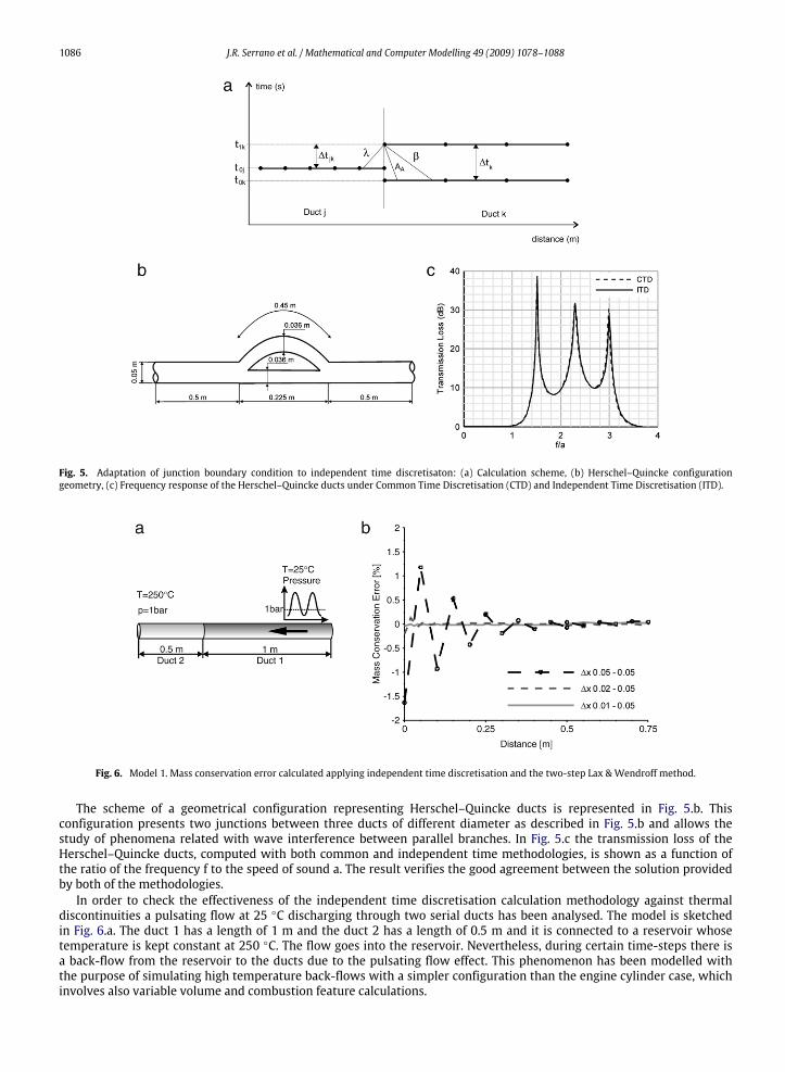
Every kind of junction between ducts can be classified into another group. In this case, when the boundary conditionis solved it must be considered that each duct connected to the boundary condition is at a different calculation time. Thissituation is represented in Fig. 5.a, which shows the resolution of the connection between two ducts. Every point representsa node of the duct; a gas velocity from right to left is assumed in the pipe.

The duct k is being solved. Its calculation time is t0k and the aim is to advance the calculation until the time t1k. For that,the thermo-fluid-dynamic properties of the duct j are available at the calculation time t0j.

In order to solve the boundary condition, the origin of the three characteristic lines has to be found, so that at thecalculation time t1k they all are passing through the extreme node of the duct k. Due to the fact that each duct is at a differenttime level, two distinct time steps 1tk and 1tjk must be considered.

1086 J.R. Serrano et al. / Mathematical and Computer Modelling 49 (2009) 1078–1088

Fig. 5. Adaptation of junction boundary condition to independent time discretisaton: (a) Calculation scheme, (b) Herschel–Quincke configurationgeometry, (c) Frequency response of the Herschel–Quincke ducts under Common Time Discretisation (CTD) and Independent Time Discretisation (ITD).

Fig. 6. Model 1. Mass conservation error calculated applying independent time discretisation and the two-step Lax & Wendroff method.

The scheme of a geometrical configuration representing Herschel–Quincke ducts is represented in Fig. 5.b. Thisconfiguration presents two junctions between three ducts of different diameter as described in Fig. 5.b and allows thestudy of phenomena related with wave interference between parallel branches. In Fig. 5.c the transmission loss of theHerschel–Quincke ducts, computed with both common and independent time methodologies, is shown as a function ofthe ratio of the frequency f to the speed of sound a. The result verifies the good agreement between the solution providedby both of the methodologies.

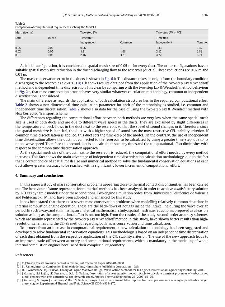
In order to check the effectiveness of the independent time discretisation calculation methodology against thermaldiscontinuities a pulsating flow at 25 ◦C discharging through two serial ducts has been analysed. The model is sketchedin Fig. 6.a. The duct 1 has a length of 1 m and the duct 2 has a length of 0.5 m and it is connected to a reservoir whosetemperature is kept constant at 250 ◦C. The flow goes into the reservoir. Nevertheless, during certain time-steps there isa back-flow from the reservoir to the ducts due to the pulsating flow effect. This phenomenon has been modelled withthe purpose of simulating high temperature back-flows with a simpler configuration than the engine cylinder case, whichinvolves also variable volume and combustion feature calculations.

J.R. Serrano et al. / Mathematical and Computer Modelling 49 (2009) 1078–1088 1087

Table 2Comparison of computational requirements solving the Model 1

Mesh size (m) Two-step LW Two-step LW+ FCT

Duct 1 Duct 2 Time unit Time unitIndependent Common Independent Common

0.05 0.05 0.96 1 1.33 1.420.02 0.05 1.31 1.68 2.12 2.830.01 0.05 2.46 3.21 4.72 6.71

As initial configuration, it is considered a spatial mesh size of 0.05 m for every duct. The other configurations have asuitable spatial mesh size reduction in the duct discharging flow to the reservoir (duct 2). These reductions are 0.02 m and0.01 m.

The mass conservation error in the ducts is shown in Fig. 6.b. The distance takes its origin from the boundary conditiondischarging to the reservoir at 250 ◦C. Fig. 6.b shows results obtained from the application of the two-step Lax & Wendroffmethod and independent time discretisation. It is clear by comparing with the two-step Lax & Wendroff method behaviourin Fig. 2.c, that mass conservation error behaves very similar whatever calculation methodology, common or independentdiscretisation, is considered.

The main difference as regards the application of both calculation structures lies in the required computational effort.Table 2 shows a non-dimensional time calculation parameter for each of the methodologies studied, i.e. common andindependent time discretisation. Table 2 shows also data for the case of using the two-step Lax & Wendroff method withFlux Corrected Transport scheme.

The differences regarding the computational effort between both methods are very low when the same spatial meshsize is used in both ducts and are due to different wave speed in the ducts. They are explained by slight differences inthe temperature of back-flows in the duct next to the reservoir, so that the speed of sound changes in it. Therefore, sincethe spatial mesh size is identical, the duct with a higher speed of sound has the most restrictive CFL stability criterion. Ifcommon time discretisation is applied, this duct sets the time-step of the model. On the contrary, the use of independenttime discretisation allows the duct not connected to the reservoir to be calculated by using a greater time-step, due to itsminor wave speed. Therefore, this second duct is not calculated so many times and the computational effort diminishes withrespect to the common time discretisation approach.

As the spatial mesh size of the duct next to the reservoir is reduced, the computational effort needed by every methodincreases. This fact shows the main advantage of independent time discretisation calculation methodology, due to the factthat a correct choice of spatial mesh size and numerical method to solve the fundamental conservation equations at eachduct allows greater accuracy to be reached, with a significantly lower increment of computational effort.

4. Summary and conclusions

In this paper a study of mass conservation problems appearing close to thermal contact discontinuities has been carriedout. The behaviour of some representative numerical methods has been analysed, in order to achieve a satisfactory solutionby 1-D gas dynamic models under these conditions. Two engine simulation codes, from Universidad Politécnica de Valenciaand Politecnico di Milano, have been adopted and enhanced for this study.

It has been stated that there exist severe mass conservation problems when modelling relatively common situations ininternal combustion engine operation. These are the back-flows of hot gas inside the intake line during the valve overlapperiod. In such a way, and still missing an analytical mathematical study, spatial mesh size reduction is proposed as a feasiblesolution as long as the computational effort is not too high. From the results of the study, second-order accuracy schemes,which are mainly represented by the two-step Lax & Wendroff method in this study, have shown better results than high-resolution schemes and the CE–SE method regarding both mass conservation and time calculation.

To protect from an increase in computational requirement, a new calculation methodology has been suggested anddeveloped to solve fundamental conservation equations. This methodology is based on an independent time discretisationof each duct obtained from the respective application of the CFL stability criterion. The use of the new approach leads toan improved trade-off between accuracy and computational requirements, which is mandatory in the modelling of wholeinternal combustion engines because of their complex duct geometry.

References

[1] T. Johnson, Diesel emission control in review, SAE Technical Paper 2006-01-0030.[2] J.I. Ramos, Internal Combustion Engine Modelling, Hemisphere Publishing Corporation, 1989.[3] D.E. Winterbone, R.J. Pearson, Theory of Engine Manifold Design: Wave Action Methods for IC Engines, Professional Engineering Publishing, 2000.[4] J. Galindo, J.M. Luján, J.R. Serrano, V. Dolz, S. Guilain, Description of a heat transfer model suitable to calculate transient processes of turbocharged

diesel engines with one-dimensional gas-dynamic codes, Applied Thermal Engineering 26 (2006) 66–76.[5] J. Galindo, J.M. Luján, J.R. Serrano, V. Dolz, S. Guilain, Design of an exhaust manifold to improve transient performance of a high-speed turbocharged

diesel engine, Experimental Thermal and Fluid Science 28 (2004) 863–875.

1088 J.R. Serrano et al. / Mathematical and Computer Modelling 49 (2009) 1078–1088

[6] G. Montenegro, F. Piscaglia, A. Onorati, G. Catalano, P. Cioffi, A 1D unsteady thermo-fluid dynamic approach for the simulation of the hydrodynamicsof diesel particulate filters, SAE Technical Paper 2006-01-0262.

[7] F. Piscaglia, G. Montenegro, A. Onorati, A 1D unsteady thermo-dynamic approach for the simulation of diesel particulate filters., in: THIESEL 2006 Int.Conference on Thermo- and Fluid Dynamic Processes in Diesel Engines, Valencia, Spain, 2006.

[8] F. Payri, A.J. Torregrosa, M.D. Chust, Application of MacCormack schemes to IC engine exhaust noise prediction, Journal of Sound and Vibration 195(5) (1996) 757–773.

[9] A. Onorati, A white noise approach for rapid gas dynamic modeling of IC engine silencers, in: Third International Conference on Computers inReciprocating Engines and Gas Turbines 1996-01, Institution of Mechanical Engineers, Mechanical Engineering Publications, 1996, pp. 219–228.C499/052.

[10] A. Onorati, Numerical Simulation of Unsteady Flows in I.C. Engine Silencers and the Prediction of Tailpipe Noise, Professional Engineering Publishing,London, 1999, Ch. 6.

[11] F. Payri, E. Reyes, J.R. Serrano, A model for load transients of turbocharged diesel engines, SAE Technical Paper 1999-01-0225.[12] F. Payri, J. Benajes, J. Galindo, J.R. Serrano, Modelling of turbocharged diesel engines in transient operation. Part 2: Wave action models for calculating

the operation in a high speed direct injection engine, in: Proceedings of the Institution of Mechanical Engineers, Part D: Journal of AutomobileEngineering 216 (2002) 479–493.

[13] N. Watson, Computers in diesel engine turbocharging system design, in: Institution of Mechanical Engineers Conference International ConferenceComputers in Engine Technology 1987-1, Institution of Mechanical Engineers, 1987, pp. 269–280, C05/87.

[14] D.E. Winterbone, M. Yoshitomi, The accuracy of calculating wave action in engine intake manifolds, SAE Technical Paper 900677.[15] M.D. Roselló, J.R. Serrano, X. Margot, J.M. Arnau, Analytic-numerical approach to flow calculation in intake and exhaust systems of internal combustion

engines, Mathematical and Computer Modelling 36 (2002) 33–45.[16] E. Ponsoda, J.V. Romero, J.R. Serrano, J.M. Arnau, A new iterative method for flow calculation inintake and exhaust systems of internal combustion

engines, Mathematical and Computer Modelling 38 (2003) 99–111.[17] J.M. Arnau, E. Navarro, M.D. Roselló, F.J. Arnau, An iterative method to obtain analytical-numerical approximation of the one-dimensional gas flow

transport solution in conical ducts, Mathematical and Computer Modelling 41 (2005) 407–416.[18] R.J. Pearson, D.E. Winterbone, Calculation of one-dimensional unsteady flow in internal combustion engine. How long should it take? in: Third

International Conference on Computers in Reciprocating Engines and Gas Turbines 1996-01, Institution of Mechanical Engineers, MechanicalEngineering Publications, 1996, pp. 193–202. C499/012.

[19] R.S. Benson, The Thermodynamics and Gas Dynamics of Internal-Combustion Engines, vol. 1, Clarendon Press Oxford, 1982.[20] R. Courant, E. Isaacson, M. Rees, On the solution of nonlinear hyperbolic differential equations by finite differences, Communications on Pure and

Applied Mathematics 5.[21] P.D. Lax, Weak solutions of non linear hyperbolic equations and their numerical computation, Communications on Pure and Applied Mathematics 7

(1954) 159–193.[22] P.D. Lax, B. Wendroff, Systems of conservation laws, Communications on Pure and Applied Mathematics 17 (1964) 381–398.[23] R.D. Richtmyer, K.W. Morton, Difference methods for initial value problems, Interscience, New York.[24] R.W. MacCormack, The effect of viscosity in hypervelocity impact cratering, AIAA Paper (1969-354).[25] S.K. Godunov, A difference scheme for numerical computation of discontinuous solutions of hydrodynamics equations, Mathematics of the USSR-

Sbornik 47 (1959) 271–306. english translation in US Joint Publication Research Service, JPRS 7226, 1969.[26] J.L. Steger, R.F. Warming, Flux vector splitting of the inviscid gas dynamic equations with application to finite-difference methods, Journal of

Computational Physics 40 (1981) 236–293.[27] J.P. Boris, D.L. Book, Flux-corrected transport. I SHASTA, a fluid transport algorithm that works, Journal of Computational Physics 11 (1973) 38–69.[28] D.L. Book, J.P. Boris, Flux-corrected transport. II Generalisations of the method, Journal of Computational Physics 18 (1975) 248–283.[29] H. Niessner, T. Bulaty, A family of flux-correction methods to avoid overshoot occurring with solutions of unsteady flow problems, Proceedings of the

GAMM Conference of Numerical Methods of Fluid Mechanics, 1981, pp. 241–50.[30] A. Harten, High resolution schemes using flux limiters for hyperbolic conservation laws, Journal of Computational Physics 49 (1983) 357–393.[31] S.C. Chang, W. To, A brief description of a new numerical framework for solving conservation laws, The method of Space-Time Conservation Element

and Solution Element, NASA Technical Memorandum 105757.[32] S.C. Chang, X.Y. Wang, C.Y. Chow, The method of space-time conservation element and solution element – aplications to one-dimensional and two-

dimensional time-marching flow problems, NASA Technical Memorandum 106915.[33] G. Briz, P. Giannattasio, Applicazione dello schema numerico Conservation Element - Solution Element al calcolo del flusso intazionario nei condotti

dei motori a c.i., in: Proc. 48th ATI National Congress, 1993, pp. 233–247 (in Italian).[34] J.M. Corberán, L. Gascón, TVD schemes for the calculation of flow in pipes of variable cross-section, Mathematical and Computer Modelling 21 (1995)

85.[35] J.M. Corberán, L. Gascón, New method to calculate unsteady 1-D compressible flow in pipes with variable cross-section. Application to the calculation

of the flow in intake and exhaust pipes of IC engines, in: Proceedings of the ASME Internal Combustion Engine Division Spring Meeting, ICE EngineModeling 23 (1995) 77–87.

[36] L. Gascón, J.M. Corberán, Construction of second-order TVD schemes for non-homogeneous hyperbolic conservation law, Journal of ComputationalPhysics 172 (2001) 261–297.

[37] J. Liu, N. Schorn, C. Schernus, L. Peng, Comparison studies on the Method of Characteristics and finite difference methods for one-dimensional gas flowthrough IC engine manifold, SAE Technical Paper 960078.

[38] M. Vandevoorde, J. Vierendeels, E. Dick, R. Sierens, A new total variation diminishing scheme for the calculation of one-dimensional flow in inlet andexhaust pipes of internal combustion engines, in: Proceedings of the Institution of Mechanical Engineers, Part D: Journal of Automobile Engineering212 (1998) 437–448.

[39] M. Poloni, D.E. Winterbone, J.R. Nichols, Comparison of unsteady flow calculations in a pipe by the method of characteristics and the two-stepdifferential Lax-Wendroff method, International Journal of Mechanical Science 29 (5) (1987) 367–378.

[40] R.J. Pearson, D.E. Winterbone, The simulation of gas dynamics in engine manifolds using non-linear symmetric difference scheme, in: Proceedings ofthe Institution of Mechanical Engineers, Part C: Journal of Mechanical Engineering Science 211 (1997) 601–616.

[41] A. Onorati, G. D’Errico, G. Ferrari, 1D fluid dynamic modeling of unsteady reacting flows in the exhaust system with catalytic converter for S.I. engines,SAE Technical Paper 2000-01-0210.

[42] D.E. Winterbone, R.J. Pearson, Calculating the effects of variations in composition on wave propagation in gases, International Journal of MechanicalScience 35 (6) (1993) 517–537.

[43] A. Onorati, G. Ferrari, Modeling of 1-D unsteady flows in I.C. engine pipe systems: numerical methods and transport of chemical species, SAE TechnicalPaper 980782.

[44] F. Payri, J. Galindo, J.R. Serrano, F.J. Arnau, Analysis of numerical methods to solve one-dimensional fluid-dynamic governing equations under impulsiveflow in tapered ducts, International Journal of Mechanical Science 46 (2004) 981–1004.

[45] J.M. Arnau, S. Jerez, L. Jódar, J.V. Romero, A semi-implicit conservation element-solution element method for chemical species transport simulationto tapered ducts of internal combustion engine, Mathematics and Computers in Simulation 73 (2006) 28–37.

[46] R. Courant, K.O. Friedrichs, H. Lewy, Über die partiellen Differenzengleichungen der mathematischen Physik, Mathematische Annalen 100 (1928)32–74.

[47] L. Gascón, Study of finite difference schemes for compressible, one-dimensional, unsteady, non-homoentropic flow calculation, Ph.D. thesis, Univ.Politécnica de Valencia, Spain, 1995 (in Spanish).