18 969 Geometry

18.969: Topics in Geometry

Contents

1 Lecture 1 (Notes: K. Venkatram) 31.1 Smooth Manifolds . . . . . . . . . . . . . . . . . . . . . . . . . . . . . . . . . . . . . . . . . . 31.2 Geometry of Foliations . . . . . . . . . . . . . . . . . . . . . . . . . . . . . . . . . . . . . . . . 41.3 Symplectic Structure . . . . . . . . . . . . . . . . . . . . . . . . . . . . . . . . . . . . . . . . . 5

2 Lecture 2 (Notes: A. Rita) 52.1 Comments on previous lecture . . . . . . . . . . . . . . . . . . . . . . . . . . . . . . . . . . . . 52.2 Symplectic Manifolds . . . . . . . . . . . . . . . . . . . . . . . . . . . . . . . . . . . . . . . . . 52.3 Poisson geometry . . . . . . . . . . . . . . . . . . . . . . . . . . . . . . . . . . . . . . . . . . . 6

3 Lecture 3 (Notes: J. Bernstein) 83.1 Almost Complex Structure . . . . . . . . . . . . . . . . . . . . . . . . . . . . . . . . . . . . . 83.2 Hermitian Structure . . . . . . . . . . . . . . . . . . . . . . . . . . . . . . . . . . . . . . . . . 83.3 Integrability of J . . . . . . . . . . . . . . . . . . . . . . . . . . . . . . . . . . . . . . . . . . . 93.4 Forms on a Complex Manifold . . . . . . . . . . . . . . . . . . . . . . . . . . . . . . . . . . . 103.5 Dolbeault Cohomology . . . . . . . . . . . . . . . . . . . . . . . . . . . . . . . . . . . . . . . . 10

4 Lecture 4 (Notes: J. Pascaleff) 114.1 Geometry of V ⊕ V ∗ . . . . . . . . . . . . . . . . . . . . . . . . . . . . . . . . . . . . . . . . . 114.2 Linear Dirac structures . . . . . . . . . . . . . . . . . . . . . . . . . . . . . . . . . . . . . . . . 134.3 Generalized metrics . . . . . . . . . . . . . . . . . . . . . . . . . . . . . . . . . . . . . . . . . . 15

5 Lecture 5 (Notes: C. Kottke) 165.1 Spinors . . . . . . . . . . . . . . . . . . . . . . . . . . . . . . . . . . . . . . . . . . . . . . . . 165.2 The Spin Group . . . . . . . . . . . . . . . . . . . . . . . . . . . . . . . . . . . . . . . . . . . 175.3 A Bilinear Pairing on Spinors . . . . . . . . . . . . . . . . . . . . . . . . . . . . . . . . . . . . 185.4 Pure Spinors . . . . . . . . . . . . . . . . . . . . . . . . . . . . . . . . . . . . . . . . . . . . . 19

6 Lecture 6 (Notes: Y. Lekili) 196.1 Generalized Hodge star . . . . . . . . . . . . . . . . . . . . . . . . . . . . . . . . . . . . . . . 206.2 Spinors for TM ⊕ T ∗M and the Courant algebroid . . . . . . . . . . . . . . . . . . . . . . . . 21

7 Lecture 7 (Notes: N. Rosenblyum) 227.1 Exact Courant Algebroids . . . . . . . . . . . . . . . . . . . . . . . . . . . . . . . . . . . . . . 227.2 ˇ 23Severa’s Classification of Exact Courant Algebroids . . . . . . . . . . . . . . . . . . . . . . . .

8 Lecture 8 (Notes: J. Bernstein) 258.1 Dirac Structures . . . . . . . . . . . . . . . . . . . . . . . . . . . . . . . . . . . . . . . . . . . 258.2 Geometry of Lie Groups . . . . . . . . . . . . . . . . . . . . . . . . . . . . . . . . . . . . . . . 27

1

9 Lecture 9 (Notes: K. Venkatram) 279.1 Bilinar forms on groups . . . . . . . . . . . . . . . . . . . . . . . . . . . . . . . . . . . . . . . 28

9.1.1 Key calculation . . . . . . . . . . . . . . . . . . . . . . . . . . . . . . . . . . . . . . . . 28

10 Lecture 10 (Notes: K. Venkatram) 2910.1 Integrability . . . . . . . . . . . . . . . . . . . . . . . . . . . . . . . . . . . . . . . . . . . . . . 2910.2 Dirac Maps . . . . . . . . . . . . . . . . . . . . . . . . . . . . . . . . . . . . . . . . . . . . . . 2910.3 Manifolds with Courant Structure . . . . . . . . . . . . . . . . . . . . . . . . . . . . . . . . . 30

11 Lecture 11(Notes: K. Venkatram) 3111.1 Integrability and spinors . . . . . . . . . . . . . . . . . . . . . . . . . . . . . . . . . . . . . . . 3111.2 Lie Bialgebroids and deformations . . . . . . . . . . . . . . . . . . . . . . . . . . . . . . . . . 32

12 Lecture 12-17(Notes: K. Venkatram) 3312.1 Generalized Complex Structures and Topological Obstructions . . . . . . . . . . . . . . . . . 33

12.1.1 Z-grading on spinors . . . . . . . . . . . . . . . . . . . . . . . . . . . . . . . . . . . . 3512.1.2 Complex Case . . . . . . . . . . . . . . . . . . . . . . . . . . . . . . . . . . . . . . . . 3612.1.3 Symplectic Case . . . . . . . . . . . . . . . . . . . . . . . . . . . . . . . . . . . . . . . 37

12.2 Intermediate Cases . . . . . . . . . . . . . . . . . . . . . . . . . . . . . . . . . . . . . . . . . . 3812.2.1 Complex and Symplectic Decompositions . . . . . . . . . . . . . . . . . . . . . . . . . 3812.2.2 General case . . . . . . . . . . . . . . . . . . . . . . . . . . . . . . . . . . . . . . . . . 3812.2.3 Weinstein Splitting . . . . . . . . . . . . . . . . . . . . . . . . . . . . . . . . . . . . . . 3912.2.4 Examples of type jumping . . . . . . . . . . . . . . . . . . . . . . . . . . . . . . . . . . 40

12.3 Spinorial Description . . . . . . . . . . . . . . . . . . . . . . . . . . . . . . . . . . . . . . . . . 4012.3.1 More Examples of Type Jumping . . . . . . . . . . . . . . . . . . . . . . . . . . . . . . 4212.3.2 Interpolation . . . . . . . . . . . . . . . . . . . . . . . . . . . . . . . . . . . . . . . . . 4212.3.3 Intermediate Types . . . . . . . . . . . . . . . . . . . . . . . . . . . . . . . . . . . . . . 4312.3.4 Generalized K ahler Geometry . . . . . . . . . . . . . . . . . . . . . . . . . . . . . . . 44

12.4 Introduction to Hermitian Geometry . . . . . . . . . . . . . . . . . . . . . . . . . . . . . . . . 4512.4.1 Condition on Types . . . . . . . . . . . . . . . . . . . . . . . . . . . . . . . . . . . . . 4512.4.2 Integrability . . . . . . . . . . . . . . . . . . . . . . . . . . . . . . . . . . . . . . . . . . 46

13 Lecture 18 (Notes: K. Venkatram) 4713.1 Generalized K ahler Geometry . . . . . . . . . . . . . . . . . . . . . . . . . . . . . . . . . . . . 47

13.1.1 Integrability . . . . . . . . . . . . . . . . . . . . . . . . . . . . . . . . . . . . . . . . . . 47

14 Lecture 19 (Notes: K. Venkatram) 4914.1 Generalized K ahler Geometry . . . . . . . . . . . . . . . . . . . . . . . . . . . . . . . . . . . . 4914.2 Hodge Theory on Generalized K ahler Manifolds . . . . . . . . . . . . . . . . . . . . . . . . . 50

15 Lecture 20 (Notes: K. Venkatram) 5115.1 Generalized Complex Branes (of rank 1) . . . . . . . . . . . . . . . . . . . . . . . . . . . . . . 51

15.1.1 General Properties of Generalized Complex Branes . . . . . . . . . . . . . . . . . . . . 5215.1.2 Branes for Other Generalized Complex Manifolds . . . . . . . . . . . . . . . . . . . . . 53

16 Lecture 21-23 (Notes: K. Venkatram) 5316.1 Linear Algebra . . . . . . . . . . . . . . . . . . . . . . . . . . . . . . . . . . . . . . . . . . . . 53

16.1.1 Doubling Functor . . . . . . . . . . . . . . . . . . . . . . . . . . . . . . . . . . . . . . . 5416.1.2 Maps Induced by Morphisms . . . . . . . . . . . . . . . . . . . . . . . . . . . . . . . . 5416.1.3 Factorization of Morphisms L : DV → D(W ) . . . . . . . . . . . . . . . . . . . . . . . 54

16.2 T -duality . . . . . . . . . . . . . . . . . . . . . . . . . . . . . . . . . . . . . . . . . . . . . . . 54

2

� � � � � �

� �

�

� � � � � �

� � �

�

1 Lecture 1 (Notes: K. Venkatram)

1.1 Smooth Manifolds

Let M be a f.d. C∞ manifold, and C∞(M) the algebra of smooth R-valued functions. Let T = TM be the tangent bundle of M : then C∞(T ) is the set of derivations Der(C∞(M)), i.e. the set of morphisms X ∈ End(C∞(M)) s.t. X(fg) = (Xf)g + f(Xg). Then C∞(T ) is equilled with a Lie bracket [, ] via the commutator [X,Y ]f = XY f − Y Xf .

XNote. Explicitly, [X,Y ] can be obtained as limt→0 Y −Fl

t

t Y , where FlXt ∈ Diff(M) is the flow of the vector

field on M .

Definition 1. The exterior derivative is the mapping

k k+1

d : C∞ T ∗ C∞ T ∗ →

p �→ (X0, . . . , Xk) �→ (−1)iXip(X0, . . . , Xi, . . . , Xk) (1) i ⎤

+ (−1)i+j p([Xi, Xj ], X0, . . . , Xi, . . . , Xj , . . . , Xk)⎦ i<j

Since [, ] satisfies the Jacobi identity, d2 = 0, i.e.

k k+1k�−1 � � C∞ T ∗ d

C∞ T ∗ d C∞ T ∗ (2)· · · → → → → · · ·

�kis a differential complex of first-order differential operators. Set Ωk(M) = C∞( T ∗). Letting mf = {g �→fg} denote multiplication by f , one finds that [d,mf ]ρ = df ∧ ρ, thus obtaining a sequence of symbols

k−1 k k+1

T ∗ η∧· T ∗ η∧· T ∗ (3) → →

which is exact for any nonzero 1-form η ∈ C∞(T ∗). Thus, Ω∗ is an elliptic complex. In particular, if M is Ker d|Ω∗compact, H∗(M) = Im d|Ω∗−1

is finite dimensional.

Remark. d has the property d(α ∧ β) = dα ∧ dβ + (−1)deg αα ∧ dβ. Thus, (Ω•(M), d, ∧) is a differential graded algebra, and H•(M) = Hk(M) has a ring structure (called the de Rham cohomology ring).

We would like to express [X,Y ] in terms of d. Now, a vector field X ∈ C∞(T ) determines a derivation

iX : Ωk(M) → Ωk−1(M), ρ �→ [(Y1, . . . , Yk) �→ ρ(X,Y1, . . . , Yk)] (4)

of Ω∗(M). iX has degree −1 and order 0.

Definition 2. The Lie derivative of a vector field X is LX = [iX , d].

Note that this map has order 1 and degree 0.

Theorem 1 (Cartan’s formula). i[X,Y ] = [[iX , d], iY ]

3

� � � � � �

�

�

�

One thus obtains [, ] as the derived bracket of d. See Kosmann-Schwarzbach’s “Derived Brackets” for more information.

Problem. Classifly all derivations of Ω•(M), and show that the set of such derivations has the structure of a Z-graded Lie algebra.

One can extend the Lie bracket [, ] on vector fields to an operator on all C∞( �k

T ).

Definition 3. The Shouten bracket is the mapping

p q� � p+�q−1

[, ] : C∞ T × C∞ T → C∞ T

(X1 ∧ · · · ∧ Xp, Y1 ∧ · · · ∧ Yq ) �→ (−1)i+j [Xi, Yi] ∧ X1 ∧ · · · ∧ Xi ∧ · · · ∧ Xp ∧ Y1 ∧ · · · ∧ Yj ∧ · · · ∧ Yq

(5)

with the additional properties [X, f ] = −[f,X] = X(f) and [f, g] = 0∀f, g ∈ C∞(M).

Note the following properties:

[P,Q] = −(−1)(deg P −1)(deg Q−1)[Q,P ]•

• [P,Q ∧ R] = [P,Q] ∧ R + (−1)(deg P −1)deg QQ ∧ [P,R]

• [P, [Q,R]] = [[P,Q], R] + (−1)(deg P −1)(deg Q−1)[Q, [P,R]]

Thus, we find that C∞( T ) has two operations: a wedge product ∧, giving it the structure of a graded commutative algebra, and a bracket [, ], giving it the structure of the Lie algebra. The above properties imply that it is a Gerstenhaber algebra.

Finally, for P = X1 ∧ · · · ∧ Xp, define ip = iX1 ◦ · · · ◦ iXp . Note that it is a map of degree −p

Problem. Show that [[iP , d]iQ] = (−1)(deg P −1)(deg Q−1)i[P,Q].

1.2 Geometry of Foliations

Let Δ ⊂ T be subbundle of the tangent bundle (distribution) with constant rank k. �� Definition 4. An integrating foliation is a decomposition M = S of M into “leaves” which are locally embedded submanifolds with TS = Δ.

Note that such leaves all have dimension k.

Theorem 2 (Frobenius). An integrating foliation exists ⇔ Δ is involutive, i.e. [Δ, Δ] ⊂ [Δ].

A distribution is equivallently determined by Ann Δ ⊂ T ∗ or the line det Ann Δ ⊂ Ωn−k(M). That is, for locally-defined 1-forms (θ1, . . . , θn−k) s.t. Δ = Ker θi, Ω = θ1 ∧ · · · ∧ θk generates a line bundle. If Δ i is involutive, iX iY dΩ = [[iX , d], iY ]Ω = i[X,Y ]Ω = 0 for all X,Y s.t. iX Ω = iY Ω = 0. That is, dΩ = η ∧ Ω for some 1-form η ∈ Ω.

Remark. More generally, let Δ ⊂ T be a distribution on non-constant rank spanned by an nvolutive C∞(M) module D ⊂ C∞(T ) at each point. Sussmann showed that such a D gives M as a disjoint union of locally embedding leaves S with TS = Δ everywhere.

4

� �

�

� �

� �

1.3 Symplectic Structure

Definition 5. An symplectic structure on M is a closed, non-degenerate two-form ω : T T ∗.→

Let (M,ω) be a symplectic manifold: note that det ω ∈ det T ∗ ⊗ det T ∗.

Problem. Show that det ω = Pf ω ⊗ Pf ω, where Pf is the Pfaffian.

Theorem 3 (Darboux). Locally, ∃C∞ functions p1, . . . , pn, q1, . . . , qn s.t. {dpi, dqi} span T ∗ and ω = dpi ∧ dqi. That is, (M,ω) is locally diffeomorphic to (R2n , dxi ∧ dyi).

Moreover, by Stokes’ theorem, one finds that M ω ∧ · · · ∧ ω = 0 � = ⇒ [ω]i = 0 for all � i.

Corollary 1. Neither S4 nor S1 × S3 have a symplectic structure.

2 Lecture 2 (Notes: A. Rita)

2.1 Comments on previous lecture

(0) The Poincare lemma implies that the sequence

d d . . . −→C∞(∧k−1T ∗) −→ C∞(∧kT ∗) −→ C∞(∧k+1T ∗) −→ . . .

is an exact sequence of sheaves, even though it is not an exact sequence of vector spaces.

(1) We defined the Lie derivative of a vector field X to be LX = [ιX , d]. Since ιX ∈ Der−1(Ω.(M)) and d ∈ Der+1(Ω.(M)), we have

[ιX , d] = ιX d − (−1)(1)·(−1)dιX = ιX d + dιX

(2) ω : V −→ V ∗, ω∗ = −ω If ω is an isomorphism, then for any X ∈ V we have ω(X,X) = 0, so that

X ∈ Xω = Ker ω(X) = ω−1Ann X

=∼Thus, we have an isomorphism ω∗ : Xω/ �X� −→ Ann X/ �ωX� and

Ann X �X�∗ Xω ∗

= = �ωX� (Xω)∗ �X�

Then using induction, we can prove that V must be even dimensional.

2.2 Symplectic Manifolds

(continues the previous lecture) For a manifold M , consider its cotangent bundle T ∗M equipped with the 2-form ω = dθ, where θ ∈

Ω1(T ∗M)is such that θα(v) = α(π (v)). In coordinates (x1, . . . , xn, a1, . . . , an), we have θ = i aidxi and ∗

therefore dθ = dai ∧ dxi, as in the Darboux theorem. Thus, T ∗M is symplectic. i

Definition 6. A subspace W of a symplectic 2n−dimensional vector space (V, ω) is called isotropic if ω|W = 0.

W is called coisotropic if its ω-perpendicular subspace W ω is isotropic. W is called Lagrangian if it is both isotropic and coisotropic.

5

� �

There exist isotropic subspaces of any dimension 0, 1, . . . , n, and coisotropic subspaces of any dimension n, n + 1, . . . , 2n. Hence, Lagragian subspaces must be of dimension n.

We have analogous definitions for submanifolds of a symplectic manifold (M,ω):

fDefinition 7. L � (M,ω) is called isotropic if f∗ω = 0. When dim(L) = n it is called Lagrangian.→

The graph of 0 ∈ C∞(M,T ∗M ), which is the zero section of T ∗M , is Lagrangian. More generally, Γξ, the graph of ξ ∈ C∞(M,T ∗M) is a Lagrangian submanifold of T ∗M if and only if

dξ = 0. It is in this sense that we say that Lagrangian submanifolds of T ∗M are like generalized functions: f ∈ C∞(M) gives rise to df , which is a closed 1−form, so Γdf ⊂ T ∗M is Lagrangian.

Proposition 1. Suppose we have a diffeomorphism between two symplectic manifolds, ϕ : (M0, ω0) (M1, ω1) and let πi : M0 × M1 → Mi, i = 0, 1 be the projection maps.

→

Then, Graph(ϕ) ⊂ (M0 × M1, π0 ∗ω0 − π1

∗ω1) is Lagrangian if and only if ϕ is a symplectomorphism.

2.3 Poisson geometry

Definition 8. A Poisson structure on a manifold M is a section π ∈ C∞(∧2(TM)) such that [π, π] = 0, where [·, ] is the Shouten bracket. ·

Remark. [π, π] ∈ C∞(∧3(TM)), so for a surface Σ(2), all π ∈ C∞(∧2(TM)) are Poisson.

This defines a bracket on functions, called the Poisson bracket:

Definition 9. The Poisson bracket of two functions f, g ∈ C∞(∧0(TM )) is

{f, g} = π(df, dg) = ι(df ∧ dg) = [[π, f ] , g]

Proposition 2. The triple (C∞(M), ·, { , }) is a Poisson algebra, i.e., it satisfies the properties below. For f, g, h ∈ C∞(∧0(TM)),

• Leibniz rule {f, gh} = {f, g} h + g {f, h}

• Jacobi identity: {f, {g, h}} + {g, {h, f}} + {h, {f, g}} = 0

Problem. Write {f, g} in coordinates for π = πij ∂ ∂ ∂xi ∧ ∂xj .

A basic example of a Poisson structure is given by ω−1, where ω is a symplectic form on M , since

ω−1, ω−1 = 0 dω = 0 (6) ⇔

Problem. Prove (6) by testing dω(Xf , Xg, Xh), for f, g, h ∈ C∞(M).

Poisson manifolds are of interest in physics: given a function H ∈ C∞(M) on a Poisson manifold (M,π), we get a unique vector field XH = π(dH) and its flow Flt . H is called Hamiltonian, and we usually think XH

about it as energy. We have XH (H) = π(dH, dH) = 0, so H is preserved by the flow. What other functions f ∈ C∞(M)

are preserved by the flow? A function f ∈ C∞(M) is conserved by the flow if and only if XH (f) = 0, equivalently {H, f} = 0, f commutes with the Hamiltonian.

If we can find k conserved quantities, H0 = H,H1,H2, . . . ,Hk such that {H0,Hi} = 0, then the system must remain on a level surface Z = {x : (H0, . . . ,Hk) = �c} for all time. Moreover, if {Hi,Hj } for all i, j then we get commutative flows Flt . If Z is compact, connected, and k = n, then Z is a torus Tn, and the XHi

trajectory is a straight line in these coordinates. Also, Tn is Lagrangian.

6

� �

� �

Problem. Describe the Hamiltonian flow on T ∗M for H = π∗f , with f ∈ C∞(M) and π : T ∗M M . Show that a coordinate patch for M gives a natural system of n commuting Hamiltonians.

→

Let us now think about a Poisson structure, π : T ∗ → T and consider Δ = Imπ. Δ is spanned at each point x by π(df) = Xf , Hamiltonian vector fields. The Poisson tensor is always preserved:

LXf π = [π,Xf ] = [π, [π, f ]] = [[π, π] , f ] + (−1)1·1 [π, [π, f ]] = − [π, [π, f ]]

= LXf π = 0 ⇒

If Δx0 = , . . . , Xfk �, then Flt1 ◦ . . . ◦ Fltk (x0) sweeps out S � x0 submanifold of M such that �Xf1 X1 Xk

TS = Δ.

Example (of a generalized Poisson structure). Let M = g∗, for g a Lie algebra, [ 2g∗ ⊗ g. Then ·, 2

·] ∈ ∧TM = M × g∗ and T ∗M = M × g, and also ∧2(TM) = M × ∧ g, so [ ] ∈ C∞(∧2T g∗).·, ·

Given f1, f2 ∈ C∞(M), their Poisson bracket is given by {f1, f2} (x) = �[df1, df2] , x�.For f, g ∈ g linear functions on M, we have

Xf (g) = �[f, g] , x� = �adf g, x� = g, −ad∗ f x

Thus Xf = −ad∗ , so the the leaves of Δ = Imπ are coadjoint orbits. If S is a leaf, thenf

π S0 −→ NS

∗ −→ T ∗| −→ T |S −→ 0

=is a short exact sequence and we have an isomorphism π : T ∗S = TN

∗

∗|S S

∼TS, which implies that the leaf ∗ →

S is symplectic. � � Given f, g ∈ C∞(S), we can extend them to f, ˜ g ∈ C∞(M). The Poisson bracket f, ˜ g is independent � � π

of choice of f, ˜ g, so {f, g}π = f, ˜ g is well defined. ∗ π

Therefore, giving a Poisson structure on a manifold is the same as giving a “generalized” folliation with symplectic leaves.

When π is Poisson, [π, π] = 0, we can define

dπ = [π, ·] : C∞(∧kT ) → C∞(∧k+1T )

Note that [π, ] is of degree (2 − 1), so it makes sense to cal it dπ. Also,·

d2 (A) = [π, [π,A]] = [[π, π] , A] − [π, [π,A]] = − [π, [π,A]]π

= d2 = 0 ⇒ π

Thus, we have a chain complex

dπ dπ . . . −→ C∞(∧k−1T ) −→ C∞(∧kT ) −→ C∞(∧k+1T ) −→ . . .

Moreover, if mf denotes multiplication by f ∈ C∞(M),

[dπ,mf ] ψ = dπ(fψ) − fdπψ = [π, fψ] − f [π, ψ] = [π, f ] ∧ ψ = ιdf π ∧ ψ

But for any ξ ∈ T ∗, ξ = 0, (� ιξπ)∧ : ∧kT → ∧k+1T is exact only for ιξπ =� 0. So, if π is not invertible, dπ

is not an elliptic complex, and the Poisson cohomology groups, Hπk(M) = Ker dπ |∧k T /Im dπ |∧k−1T could be

infinite dimensional on a compact M . Let us look at the first such groups:

H0(M) = {f : dπf = 0} = {f : Xf = 0} = {Casimir functions, i.e. functions s.t. {f, g} = 0 for all g}π

H1(M) = {X : dπ X = 0} /Im dπ = {infinitesimal symmetries of Poisson vector fields} /Hamiltonians π

Hπ 2(M) = P ∈ C∞(∧2T ) : [π, P ] = 0 = tangent space to the moduli space of Poisson structures

7

� � � � � �

� � �

3 Lecture 3 (Notes: J. Bernstein)

3.1 Almost Complex Structure

Let J ∈ C∞(End(T )) be such that J2 = −1. Such a J is called an almost complex structure and makes the real tangent bundle into a complex vector bundle via declaring iv = J(v). In particular dim RM = 2n. This also tells us that the structure group of the tangent bundle reduces from Gl(2n, R) to Gl(n, C). Thus T is an associated bundle to a principal Gl(n, C) bundle. In particular we have map on the cohomology,

H2i(M, Z) H2i(M, Z/2Z)→

c(T, J) �→ w(T )

Where c(T, J) are the Chern classes of T (with complex structure given by J) and w(T ) are the Stiefel-Whitney classes. Here the map is reduction mod 2. In particular w2i+1 = 0 and c1 �→ w2, the later fact implies that M is Spinc .

Recall that the Pontryagin classes of a vector bundle are pi ∈ H4i such that pi(E) = (−1)ic2i(E ⊗C). We study pi(T ) = (−1)ic2i(T ⊗C). Since the eigenvalues of J : T → T are ±i we have the natural decomposition

T ⊗ C = (Ker (J − i)) ⊕ (Ker (J + i)) = T1,0 ⊕ T0,1

Here T1,0 and T0,1 =are complex subbundles of T ⊗ C and on has the identifications (T1,0, i) ∼ (T, J) and (T0,1, i) ∼= (T, −J). Hence if we choose a hermitian metric h on T we get a non degenerate pairing,

T1,0 × T0,1 → C

and hence T1,0 ∼ We now compute = (T0,1)∗.

(−1)k pk(T ) = c2k(T1,0 ⊕ T0,1) = ci(T1,0) ∪ c2k−i(T0,1) = ( ci(T1,0)) ∪ ( cj (T0,1) k k k i i j

where the last equality comes from rearranging the sum. Now we have ci(T0,1) = (−1)ici(T1,0) and since we can identity T1,0 with (T, J) we have

(−1)k pk(T ) = ( ci(T, J)) ∪ ( (−1)j cj (T, J)) k i j

Thus the existence of an almost complex structure implies that one can find classes ci ∈ H2i(M, Z) thatwhen taken mod 2 give the Stiefel-Whitney class and that satisfy the above Pontryagin relation.

Problem. Show that S4k does not admit an almost complex structure.

Remark. Topological obstructions to the existence of an almost complex structure in general are not known.

3.2 Hermitian Structure

Definition 10. A hermitian structure or a real vector space V consists of a triple

• J an almost complex structure

• ω : V → V ∗ ω symplectic (i.e. ω∗ = −ω)

g : V V ∗ g a metric (i.e. g∗ = g and if we write x �→ g(x, ) then g(x, x) > 0 for x = 0) • → · �

with the compatibility g J = ω◦

8

Now pick (J, g) this determines a hermitian structure if and only if

−(gJ) = (gJ)∗ = J∗g∗ = J∗g

. On the other hand (J, ω) determines a hermitian structure if and only if

−(ωJ) = (ωJ−1)∗ = −J∗ω∗ = J∗ω

that is if and only if J∗ω + ωJ = 0. Then we have (J∗ω + ωJ)(v)(w) = ω(Jx, y) + ω(x, Jy) = 0 which is equivalent to ω of type (1,1). We get three structure groups

g �→ O(V, g) = {A : A∗gA = g}ω �→ Sp(V, ω) = {A∗ωA = ω}J �→ Gl(V, J) = {A : AJ = JA}

Now if we form h = g + iω we obtain a hermitian metric on V . And we have structure group

Stab(h) = U(V, h) = O(v, h) ∩ Sp(V, ω) = Gl(V, J) ∩ O(V, g) = Sp(V, ω) ∩ Gl(V, J)

we note U(V, h) is the maximal compact subgroup of Gl(V, J).

Problem. 1. Show Explicitly that given J one can always find a compatible ω (or g) 2. Show similarly that givne ω can find compatible g.

3.3 Integrability of J

Since we have a Lie bracket on T we can tensor it with C and obtain a Lie bracket on T ⊗ C. The since T ⊗ C = T1,0 ⊕ T0,1, integrability conditions are thus that the complex distribution T1,0 is involutive i.e. [T1,0, T1,0] ⊆ T1,0. How far is this geometry from usual complex structure on Cn? Idea is if one can form MC

the complexification of M (think of RP n ⊂ CP n or Rn ⊂ Cn, indeed if M is real analytic it is always possible to do this. Then MC has two transverse foliations by the integrabrility condition (from T1,0 and T0,1). Say

i 1 2 nfunctions z : MC C cut out the leaves of T1,0 (i.e. the leaves are given by z = z = . . . = z = c).→ 1 nThen when one restricts the zii to a neighborhood U ⊆ M , obtains maps z , . . . , z : U → C such that

< dz1, . . . , dzn >= T1∗ ,0 = Ann(T0,1. That is one obtains a holomorphic coordinate chart. Moreover in this

chart one has � ∂ ∂ J = i(dzk ⊗

∂zk + dz k ⊗

∂z)

k k

Remark. This is similar to the Darboux theorem of symplectic geometry

More generally we have

Theorem 4. (Newlander-Nirenberg) If M is a smooth manifold with smooth almost complex structure J that is integrable then M is actually complex.

Note. This was most recently treated by Malgrange.

Now T1,0 closed under [, ] happens if and only if for X ∈ T,X − iJX ∈ T1,0 one has [X − iJX, Y − iJY ] = Z − iJZ. That is [X,Y ] − [JX, JY ] + J [X, JY ] + J [JX, Y ] = 0

Definition 11. We define the Nijenhuis tensor as NJ (X,Y ) = [X,Y ] − [JX, JY ] + J [X, JY ] + J [JX, Y ]

Problem. Show that NJ is a tensor in C∞( �2

T ∗ ⊗ T ).

Thus one has J integrable if and only if NJ = 0.

9

�

��

� �

�

Remark. NJ =0 is the analog of dω ∈ C∞( �3

T ∗)

Now if we view J ∈ End(T ) = Ω1(T ) = ξi then J acts on differential forms, ρ ∈ Ω·(M) by � � ⊗ νi

ıJ (ρ) = ξi ∧ ıvi ρ = (eξi ıvi )ρ. And one computes ·

ıJ (α ∧ β) = ıJ (α) ∧ β + (−1)αα ∧ ıJ β

thus ıJ ∈ Der0(Ω·(M)) and we may form LJ = [ıJ , d] ∈ Der1(Ω·(M)).

Note. LJ is denoted dc

Definition 12. We define the Nijenhuis bracket [, ] : Ωk × Ωl → Ωk+l by L[J,K] = [LJ , LK ]

One checks [LJ , LJ ] = LNJ hence NJ = [J, J ].

3.4 Forms on a Complex Manifold

In a manner similar with our treatment of foliations, we wish to express integrability in terms of differentiable forms. Let T0,1 (or T1,0) be closed under the complexified Lie bracket. Since Ann T0,1 = T1

∗ ,0 =< θ1, . . . , θn >

(Ann T1,0 = T1∗ ,0), Ω = θ1 ∧ . . . θn is a generator for det T1

∗ ,0 = K. Where here K is a complex line

bundle. The condition for integrability is then dΩn,0 = ξ0,1 ∧ Ωn,0 for some ξ. Taking d again one obtains 0 = dξ ∧ Ωn,0 − ξ ∧ dΩ = dξ ∧ Ω, hence ∂ξ = 0. We call K = n

T ∗ the canonical bundle.1,0

Note. This definition is deserved since K ⊂ T ∗ ⊗C and T0,1 = AnnK = {X ıX Ω = 0}, i.e. we can recover the complex structure from K

More fully, there is a decomposition of forms

· p q� � � �� T ∗ ⊗ C = T1

∗ ,0 T0

∗ ,1

p,q

Ω· = Ωp,q(M) p,q

that is a Z × Z grading. Since dΩn,0 = ξ ∧ Ω we have integrability if and only if d = ∂ + ∂, where here ∂ = πp,q+1 ◦ d and

∂ = πp+1,q ◦ d.

Problem. Show that without integrability

d = ∂ + ∂ + dN

where NJ ∈ ∧2T ∗ ⊗ T and dN = ıNJ . Also determine the p, q decomposition of dN .

3.5 Dolbeault Cohomology

Assuming NJ = 0 one has ∂2 = ∂ 2

= ∂∂ + ∂∂ = 0. Thus one gets a complex

∂ : Ωp,q(M) Ωp,q+1(M).→

The cohomology of this complex is called the Dolbeault cohomology and is denoted

Ker ∂|Ωp,q

= H∂

p,q (M ). Im ∂|Ωp,q−1

10

� �

This is a Z × Z graded ring. The symbol of ∂ can be determined from the computation [∂,mf ] = e Now ∂f . given a real form ξ ∈ T ∗ − {0} then

p,q p,q+1

T ∗ T ∗ →

ρ ξ0,1�→ ∧ ρ

is elliptic, since ξ = ξ1,0 + ξ0,1 = ξ1,0 + ξ0.1 (as ξ real) and so ξ0,1 = 0. Hence dim � Hp,q < ∞ on M compact. ∂

Now suppose E M is a complex vector bundle, how does pone make E compatible with the complex →structure J on M?

Definition 13. E M a complex vector bundle is a holomorphic if there exists a connection ∂E : C∞(E)→ 2

→

C∞(T0∗ ,1 ⊗ E) which is flat (i.e. ∂E = 0).

This gives us a complex

C∞(T0∗ ,1 ⊗ E) → . . . → Ω0,q(E) = C∞(∧0,qT ∗ ⊗ E) → . . .

The cohomology of this complex is called Dolbeault cohomology with values in E and is denoted Hq (M,E).∂E

Elliptic theory tells us that M compact implies H∂

q

E (M,E) is finite dimensional. We note that ∂|Ωn,0 is a

holomorphic structure on K and hence K is a holomorphic line bundle.

Problem. Find explicitly the ∂E operator on E = T1,0

4 Lecture 4 (Notes: J. Pascaleff)

4.1 Geometry of V ⊕ V ∗

Let V be an n-dimensional real vector space, and consider the direct sum V ⊕ V ∗. This space has a naturalsymmetric bilinear form, given by

1 �X + ξ, Y + η� = 2(ξ(Y ) + η(X))

for X,Y ∈ V , ξ, η ∈ V ∗. Note that the subspaces V and V ∗ are null under this pairing. Choose a basis e1, e2, . . . , en of V , and let e1, e2, . . . , en be the dual basis for V ∗. Then the collection

e1 + e 1 , e2 + e 2 , . . . , en + e n , e1 − e 1 , e2 − e 2 , . . . , en − e n

is a basis for V ⊕ V ∗, and we have �ei + e i , ei + e i� = 1

�ei − e i , ei − e i� = −1,

whereas for i = j,��ei ± e i , ej ± ej � = 0

Thus the pairing �·, ·� is non-degenerate with signature (n, n), a so-called “split signature.” The symmetry group of the structure consisting of V ⊕ V ∗ with the pairing �·, ·� is therefore

O(V ⊕ V ∗) = {A ∈ GL(V ⊕ V ∗) : �A = O(n, n)., A·� = �·, ·�} ∼·

Note that O(n, n) is not a compact group.

11

� �

� �

� �

We have a natural orientation on V ⊕ V ∗ coming from the canonical isomorphisms

det (V ⊕ V ∗) = det V ⊗ det V ∗ = R.

The symmetry group of V ⊕ V ∗ therefore naturally reduces to SO(n, n). The Lie algebra of SO(V ⊕ V∗) is

so(V ⊕ V ∗) = {Q : �Q·, ·� + �·, Q·�}.

By way of the non-degenerate bilinear form on V ⊕ V ∗, we may identify V ⊕ V ∗ with its dual, and so we may write

so(V ⊕ V ∗) = {Q : Q + Q∗ = 0}.

We may decompose Q ∈ so(V ⊕ V ∗) in view of the splitting V ⊕ V ∗:

A β Q = ,

B D

where A : V → V β : V ∗ → V B : V V ∗ D : V ∗ V ∗ → →

The condition that Q + Q∗ = 0 means now

D∗ β∗ Q∗ = = −Q,

B∗ A∗

or D∗ = −A, β∗ = −β, and B∗ = −B. The necessary and sufficient conditions that A, β,B,D give an element of so(V ⊕ V ∗) are therefore

A ∈ EndV, β ∈ ∧2V, B ∈ ∧2V ∗, D = −A∗.

Thus we may identify so(V ⊕ V ∗) with

End(V ) ⊕ ∧2V ⊕ ∧2V ∗.

This decomposition is consistent with the fact that, for any vector space E with a non-degenerate symmetric bilinear form �·, ·�, we have

so(E) = ∧2E.

In the case of E = V ⊕ V ∗ this gives

so(V ⊕ V ∗) = ∧2(V ⊕ V ∗) = ∧2V ⊕ (V ⊗ V ∗) ⊕ ∧2V ∗,

and the term V ⊗ V ∗ is just End(V ). Of particular note is the fact that the “usual” symmetries End(V ) of V are contained in the symmetries

of V ⊕ V ∗. (Since V is merely a vector space with no additional structure, its symmetry group is GL(V ), with Lie algebra gl(V ) = End(V ).)

Now we examine how the different parts of the decomposition

so(V ⊕ V ∗) = End(V ) ⊕ ∧2V ⊕ ∧2V ∗

act on V ⊕ V ∗. Any A ∈ End(V ) corresponds to the element

A 0 QA = 0 −A∗ ∈ so(V ⊕ V ∗).

12

� �

� �

� �

� � � � � � � �

� � � � � �

� �

� � � � � �

Which acts on V ⊕ V ∗ as the linear transformation

eA 0 eQA = 0 ((eA)∗)−1 ∈ SO(V ⊕ V ∗)

Since any transformation T ∈ GL+(V ) of positive determinant is eA for some A ∈ End(V ). We can regard GL+(V ) as a subgroup of SO(V ⊕ V ∗). In fact the map

P 0 P �→ 0 (P ∗)−1

gives an injection of GL(V ) into SO(V ⊕ V ∗). Thus, once again, the usual symmetries GL(V ) may be regarded as part of a larger group of symmetries,

namely SO(V ⊕ V ∗). This is the direct analog of the same fact at the level of Lie algebras. Now consider a 2-form B ∈ ∧2V ∗. This element corresponds to

0 0 QB =

B 0 ∈ so(V ⊕ V ∗),

which acts V ⊕ V ∗ as the linear transformation

0 0 1 0 0 0 1 0 e B = eQB = exp

B 0 = 0 1 + B 0

+ 0 = B 1

,

since Q2 = 0. More explicitly, eQ is the map B B

X X X ξ �→

ξ + B(X) = ξ + iX B

.

Thus B gives rise to a shear transformation which preserves the projection onto V . These transformations are called B-fields.

The case of a bivector β ∈ ∧2V is analogous to that of a 2-form: β corresponds to

0 β Qβ = 0 0

which acts on V ⊕ V ∗ as β Qβ

1 β X X + iξβ e = e = : ,0 1 ξ

�→ ξ

or in other words a shear transformation preserving projection onto V ∗. These are called β-field transformations.

In summary, the natural structure of V ⊕ V ∗ is such that we may regard three classes of objects defined on V , namely, endomorphisms, 2-forms, and bivectors, as orthogonal symmetries of V ⊕ V ∗.

4.2 Linear Dirac structures

A subspace L ⊂ V ⊕ V ∗ is called isotropic if

�x, y� = 0 for all x, y ∈ L.

If V has dimension n, then the maximal dimension of an isotropic subspace in V ⊕ V ∗ is n. Isotropic subspaces of the maximal dimension are called linear Dirac structures on V .

Examples of linear Dirac structures on V are

13

1. V

2. V ∗.

3. eB V = {X + iX B : X ∈ V }, which is simply the graph ΓB of the map B : V V ∗.→

4. eβ V ∗ = {iξβ + ξ : ξ ∈ V ∗}.·

5. In general, A V , where A ∈ O(V ⊕ V ∗).·

Exercise. If D is a linear Dirac structure on V , such that the projection onto to V , πV (D) = V , then there is a unique B : V → V ∗ such that D = eB V . Specifically B = πV ∗ ◦ (πV |D)−1 .

A further example of a linear Dirac structure is given as follows: let Δ ⊂ V be any subspace of dimension d. Then the annihilator of Δ, Ann(Δ), consisting of all 1-forms which vanish on Δ is a subspace of V ∗ of dimension n − d. The space

D = Δ ⊕ Ann(Δ) ⊂ V ⊕ V ∗

is then isotropic of dimension n, and is hence a linear Dirac structure. When we apply a B-field to a Dirac structure of this kind, we get

e B (Δ ⊕ Ann(Δ)) = {X + ξ + iX B : X ∈ Δ, ξ ∈ Ann(Δ)}

= e B (Δ) ⊕ Ann(Δ).

We define the type of a Dirac structure D to be codim(πV (D)). The computation above shows that a B-field transformation cannot change the type of a Dirac structure.

What matters in this computation is not so much B itself as it is the pullback f∗B of B under the inclusion f : Δ V . Indeed, if f∗B = f∗B�, then →

0 = iX (f∗B − f∗B�) = f∗(iX B − iX B�).

This means that iX B − iX B� ∈ Ann(Δ), and so

e B (Δ) ⊕ Ann(Δ) = e B� (Δ) ⊕ Ann(Δ).

Generalizing this observation, let f : E → V be the inclusion of a subspace E of V , and let � ∈ ∧2E∗. Then define

L(E, �) = {X + ξ ∈ E ⊕ V ∗ : f∗ξ = iX �},

which is a linear Dirac structure. Note that when � = 0,

L(E, 0) = E ⊕ Ann(E).

Otherwise, L(E, �) is a general Dirac structure. Conversely, the subspace E and 2-form � may be reconstructed from a given Dirac structure L. Set

E = πV (L) ⊂ V.

Then L ∩ V ∗ = {ξ : �ξ, L� = 0}

= {ξ : ξ(πV (L)) = 0}

= Ann(E).

14

We can define a map from E to V ∗/L ∩ V ∗ by taking e ∈ E first to (πV |L)−1(e) ∈ L, and then projecting onto V ∗/L ∩ V ∗; this yields

� : E → V ∗/L ∩ V ∗ = V ∗/Ann(E) = E∗.

Then we have � ∈ ∧2E∗, and L = L(E, �). In an analogous way, we could consider Dirac structures L = L(F, γ), where F = πV ∗ (L), and γ : F F ∗.→

Exercise. Let Dirk(V ) be the space of Dirac structures of type k. Determine dim Dirk(V ). Compare this to the usual stratification of the Grassmannian Grk(V ).

A B-field transformation cannot change the type of a Dirac structure, since

e B L(E, �) = L(E, � + f∗B).

However, a β-field transform can. Express a given Dirac structure L as L(F, γ), with g : F V ∗ an inclusion, and γ ∈ ∧2F ∗. Let E = πV (L), which contains L ∩ V = Ann(F ). Thus

→

E/L ∩ V = E/Ann(F ) = Im γ,

and so dim E = dim L ∩ V + rank γ.

Since rank γ is always even, if we change γ to γ + g∗β, we can change dim E by an even amount. The space Dir(V ) of Dirac structures has two connected components, one consisting of those of even

type, and one consisting of those of odd type.

4.3 Generalized metrics

There is another way to see the structure of Dir(V ). Let C+ ⊂ V ⊕ V ∗ be a maximal subspace on which the pairing �·, ·� is positive definite, e.g., the space spanned by ei + ei , i = 1, . . . , n. Let C− = C⊥ be the + orthogonal complement. Then �·, ·� is negative definite on C−.

If L is a linear Dirac structure, then L ∩ C = {0}, since L is isotropic. Thus L defines an isomorphism. ±

L : C+ → C−

such that −�Lx,Ly� = �x, y�, since �x + Lx, y + Ly� = 0. By choosing isomorphism between C± and Rn

with the standard inner product, any L ∈ Dir(V ) may be regarded as an orthogonal transformation of Rn , and conversely. Thus Dir(V ) is isomorphic to O(n) as a space. The two connected components of O(n) correspond in some way to the two components of Dir(V ) consisting of Dirac structures of even and odd type.

Observe that because C+ is transverse to V and V ∗, the choice of C+ is equivalent to the choice of a map γ : V → V ∗ such that the graph Γγ is a positive definite subspace, i.e., for 0 =� x ∈ V ,

�x + γ(x), x + γ(x)� = γ(x, x) > 0.

Thus if we decompose γ into g + b, where g is the symmetric and b the anitsymmetric part, then g must be a positive definite metric on V . The form g + b is called a generalized metric on V . A generalized metric defines a positive definite metric on V ⊕ V ∗, given by

�·, ·�|C+ − �·, ·�|C−

Exercise. Given A ∈ O(n), determine explicitly the Dirac structure LA determined by the map O(n) Dir(V ).

→

15

� �

�

�

�

�

5 Lecture 5 (Notes: C. Kottke)

5.1 Spinors

We have a natural action of V ⊕ V ∗ on ·V ∗. Indeed, if X + ξ ∈ V ⊕ V ∗ and ρ ∈ ·

V ∗, let

(X + ξ) ρ = iX ρ + ξ ∧ ρ.· Then

(X + ξ)2 ρ = iX (iX ρ + ξ ∧ ρ) + ξ ∧ (iX ρ + ξ ∧ ρ)· = (iX ξ)ρ − ξ ∧ iX ρ + ξ ∧ iX ρ

= �X + ξ,X + ξ�ρ

where �, � is the natural symmetric bilinear form on V ⊕ V ∗: 1 �X + ξ, Y + η� = 2(ξ(Y ) + η(X)).

Thus we have an action of v ∈ V ⊕ V ∗ with v2ρ = �v, v�ρ. This is the defining relation for the Clifford Algebra CL(V ⊕ V ∗).

For a general vector space E, CL(E, �, �) is defined by

CL(E, �, �) = E/ �v ⊗ v − �v, v�1�

That is, CL(E, �, �) is the quotient of the graded tensor product of E by the free abelian group generated by all elements of the form v ⊗ v − �v, v�1 for v ∈ E. Note in particular that if �, � ≡ 0 then CL(E, �, �) = ·

E. =We therefore have representation CL(V ⊕ V ∗) −→ End( = ) where n dimV .∼ � ·

V ∗) ∼ End(R2n = This is

called the “spin” representation for CL(V ⊕ V ∗). Choose an orthonormal basis for V ⊕ V ∗, i.e. {e1 ± e1, . . . , en ± en}. The clifford algebra has a natural

volume element in terms of this basis given by

2ω ≡ (−1) n(n−1)

(e1 − e 1) (en − e n)(e1 + e 1) (en + e n).· · · · · ·

Problem. Show ω1 = 1, ωei = −eiω, ωei = −eiω, and ω 1 = 1, considering 1 as the element in

�0V ∗ acted ·

on by the clifford algebra.

The eigenspace of ω is naturally split, and we have

S+ ≡ Ker(ω − 1) = evV ∗

S− ≡ Ker(ω + 1) = �od

V ∗

The ei are known as “creation operators” and the ei as “annihilation operators”. We define the “spinors” S by �

S = ·V ∗ = S+ ⊕ S−

Here is another view. V is naturally embedded in V ⊕ V ∗, so we have

CL(V ) = ·V ⊂ CL(V ⊕ V ∗)

since �V, V � = 0. Note in particular that det V ⊂ CL(V ⊕ V ∗), where detV is generated by e1 · · · en in terms of our basis elements. detV is a minimal ideal in CL(V ⊕ V ∗), so CL(V ⊕ V ∗) detV ⊂ CL(V ⊕ V ∗).· Elements of CL(V ⊕ V ∗) det V are generated by elements which look like ·

(1, e i , e i ej , . . .) en� �� e1 · · · �� no ei ≡ f ∈ det V

For x ∈ CL(V ⊕ V ∗) and ρ ∈ S, the action x ρ satisfies xρf = (x ρ)f .· · Problem. Show that this action coincides with the Cartan action.

16

� � � �

� � � �

5.2 The Spin Group

The spin group Spin(V ⊕ V ∗) ⊂ CL(V ⊕ V ∗) is defined by

Spin(V ⊕ V ∗) = {v1 · · · vr : vi ∈ V ⊕ V ∗, �vi, vi� = ±, r even.}

Spin(V ⊕ V ∗) is a double cover of the special orthogonal group SO(V ⊕ V ∗); there is a map

2:1 ρ : Spin(V ⊕ V ∗) −→ SO(V ⊕ V ∗)

where the action ρ(x) v = xvx−1 in CL(V ⊕ V ∗).· The adjoint action in the Lie algebra so(V ⊕ V ∗) is given by

dρx : v �−→ [x, v]

where [, ] is the commutator in CL(V ⊕ V ∗), so

so(V ⊕ V ∗) = span{[x, y] : x, y ∈ V ⊕ V ∗} ∼�2(V ⊕ V ∗).=

Recall that �2(V ⊕ V ∗) =

�2V ∗ ⊕

�2V ⊕ End(V ), so a generic element in

�2(V ⊕ V ∗) looks like

B + β + A ∈ �2V ∗ ⊕

�2V ⊕ End(V )

In terms of the basis, say B = Bij ei ∧ej , βij ei ∧ej , and A = Ai

j ei ⊗ej . In CL(V ⊕V ∗), these become Bij eiej ,

βij ej ei and 12 A

ji (ej e

i − eiej ), respectively. Consider the action of each type of element on the spinors.

(Bij e i ej ) ρ = Bij e

i ∧ ei ∧ ρ = −B ∧ ρ·

(βij ej ei) ρ = βij iej iei ρ = iβ ρ·

1 Aj (ej e

i i ej ) ρ =1 Aj (iej (e

i i ρ) = ( 1 Aj δi j i 1

TrA2 i − e ·

2 i ∧ ρ) − e ∧ iej 2 i j )ρ − Ai e ∧ ej ρ =2

ρ − A∗ρ

Given B ∈ �2V ∗, recall the B field transform e−B . This acts on the spinors via

1 e−B · ρ = ρ + B ∧ ρ +

2! B ∧ B ∧ ρ + · · ·

Note that there are only finitely many terms in the above. Similarly, given β ∈

�2V , we have

1 e β ρ = ρ + iβ ρ + iβ iβ ρ +·

2 · · ·

For A ∈ End(V ), eA ≡ g ∈ GL+(V ), we have

g ρ = det(g) g∗−1 ρ· ·

so that, as a GL+(V ) representation, S ∼= ·V ∗ ⊗ (detV )1/2 .

17

� � �

�

� �

� �

�

5.3 A Bilinear Pairing on Spinors

Let ρ, φ ∈ ·V ∗ and consider the reversal map α : ·

V ∗ → ·V ∗ where

αξ1 ∧ · · · ∧ ξk �−→ ξk ∧ · · · ∧ ξ1

Define (ρ, φ) = [α(ρ) ∧ φ]n ∈ detV ∗

where n = dim V , and the subscript n on the bracket indicates that we take only the degree n parts of the resulting form.

Proposition 3. For x ∈ CL(V ⊕ V ∗), (x ρ, φ) = (φ, α(x) φ)· ·

Proof. Recall that (x ρ)f = xρf and·

(ρ, φ) = if (ρ, φ)f

= if (α(ρ) ∧ φ))f

= α(f)α(ρ)φf

= α(ρf)φf

so (x ρ, φ) = α(xρf)φf = α(ρf)α(x)φf = (ρ, α(x)φ).·

Corollary 2. We have (v ρ, v φ) = (ρ, α(v)v φ) = �v, v�(ρ, φ)· · ·

Also, for g ∈ Spin(V ⊕ V ∗), (g ρ, g φ) = ±1(ρ, φ)· ·

Example. Suppose n = 4, and ρ, φ ∈ evV ∗, so that

ρ = ρ0 + ρ2 + ρ4

and similarly for φ, where the subscripts indicate forms of degree 0, 2, and 4. Then α(ρ) = ρ0 − ρ2 + ρ4 and

(ρ, φ) = (ρ0 − ρ2 + ρ4) ∧ (φ0 + φ2 + φ4) = ρ0φ4 + φ0ρ4 − ρ2 ∧ φ24

If n = 4 and ρ, φ ∈ �od

V ∗, then

(ρ, φ) = (ρ1 − ρ3) ∧ (φ1 + φ3) = ρ1 ∧ φ3 − ρ3 ∧ φ1.4

2Proposition 4. In general, (ρ, φ) = (−1) n(n−1)

(φ, ρ)

Problem. • What is the signature of (, ) when symmetric?

• Show that (, ) is non-degenerate on S±.

• Show that in dimension 4, the 16 dimensional space ·V ∗ has a non degenerate symmetric form

18

� 5.4 Pure Spinors

Let φ ∈ ·V ∗ be any nonzero spinor, and define the null space of φ as

Lφ = {X + ξ ∈ V ⊕ V ∗ : (X + ξ) φ = 0}.·

It is clear then that Lφ depends equivariantly on φ under the spin representation. If

φ �→ g · φ, g ∈ Spin(V ⊕ V ∗)

then Lφ �→ ρ(g)Lφ

where ρ : Spin(V ⊕ V ∗) → so(V ⊕ V ∗) as before. The key property of the null space is that it is isotropic. Indeed, if x, y ∈ Lφ we have

2�x, y�φ = (xy + yx)φ = 0.

Thus Lφ ⊂ L⊥φ . If Lφ = L⊥φ , that is, if Lφ is maximal, then φ is called “pure”. We have therefore that φ is pure if and

only if Lφ is Dirac.

Example. • Take φ = e1 ∧ · · · ∧ en . Then Lφ = V ∗.

Take 1 ∈ �0V ∗. Then L1 = V . For B

�2V ∗, then e−B 1 = 1 − B + 1/2B ∧ B + . So•

Le = eB (L1) = eB (V ) = ΓB . ∈ · · · ·

B

• For θ ∈ V ∗, θ is pure since Lθ = {X + ξ : iX θ + ξ ∧ θ = 0} = Ker θ ⊕ �θ� which is Dirac; indeed this is what we called L(Ker θ, 0).

• Similarly, considering eB θ, we have LeB θ = L(Ker θ, f∗B).

• Given a Dirac structure L(E, �), choose θ1, . . . , θk such that �θ1, . . . , θk� = Ann E. Choose B ∈ �2V ∗

such that f� ∗B = �. Then φ = e−B θ1 ∧ · · · ∧ θk is pure and Lφ = L(E, �).

Problem. • Show Lφ ∩ Lφ� = {∅} ⇔ (φ, φ�) = 0. �

Let dim V = 4, and ρ = ρ0 + ρ2 + ρ4 = 0. Show that ρ is pure iff 2ρ0ρ4• � = ρ2 ∧ ρ2.

6 Lecture 6 (Notes: Y. Lekili)

Recall from last lecture : S = Λ•V ∗, (X + ξ) ρ = ιX ρ + ξ ∧ ρ. Mukai pairing (ρ, φ) = [ρ ∧ α(φ)]n Spin0-invariant. ·

Dir(V ) Pure spinors ←→

Lφ ←→ φ = ce B θ1 ∧ . . . ∧ θk, k = type

Problem. 1. Prove that Lφ ∩ L�

= {0} ⇔ (φ, φ� ) = 0 �φ

2. Let dimV = 4. Show that 0 =� ρ = ρ0 + ρ2 + ρ4 is pure iff 2ρ0ρ4 = ρ2 ∧ ρ2. Show in general dimension that Pur = Pure spinors ⊂ S± are defined by a quadratic cone. Indentify the space P(Pur) ⊂ P(S±.)

19

� �

� �

6.1 Generalized Hodge star

C+ positive definite. C+ : V → V ∗ , C+(X)(X) > 0 for X = 0 . � C+ = Γg+b, g ∈ S2V ∗ and b ∈ Λ2V ∗. Note that C+ determines an operator

G : V ⊕ V ∗ → V ⊕ V ∗

�Gx,Gy� = �x, y�, G2 = 1. So G∗ = G. G is called a generalized metric since �Gx, y� is positive definite.

Note that if C+ = Γg : {v + g(v)} and C− = {v − g(v)} then G = g 0 g−

0

1 . In general

C+ = Γg+b = ebΓg so � � � ��

G = eb 0 g−1 e−b =

1 0 0 g−1 1 0 =

−g−1b g−1

g 0 b 1 g 0 −b 1 g − bg−1b bg−1

Problem. Note that restriction of G to T is g − bg−1b. Verify that it is indeed positive definite.

Comment about the volume form of g − bg−1b = gb :

Note: g − bg−1b = (g − b)g−1(g + b) . So det(g − bg−1b) =det(g − b)det(g−1)det(g + b), and det(g+b)det(g + b) =det(g + b)∗ =det(g − b). Hence volgb =det(g − bg−1b)1/2 = det(g)1/2 .

Problem. What is volgb /volg ?

Aside: detV ∗, choose orientation. detV ∗ ⊗ V ∗ , natural orientation since square. detg(v ⊗ v) > 0 so detghas square roots. After choice of orientation on V , there exists a unique positive square root volg.

A generalized metric is given by G : V ⊕ V ∗ → V ⊕ V ∗ such that G2 = 1, G∗ = G, �G(x), x� > 0.C± = ker(G � 1).Consider ∗ = a1 . . . an where (a1, . . . , an) is an oriented basis for C+. ∗ ∈CL(C+) ⊂CL(V ⊕ V ∗).

• ∗ is the volume element of CL(C+)

• ∗ is the lift of −G to Pin(V ⊕ V ∗) = {v1 . . . vr : ||vi|| = ±1} (Spin if n is even)

• ∗ acts on forms via ∗ · ρ = a1 . . . an · ρ. Consider b = 0 and ei, e

i orthonormal basis. Then ∗ = (e1 + e1) . . . (en + en). Consider α(∗) = (en + en) . . . (e1 + e1). α(∗)1 = en ∧ . . . ∧ e1 , α(∗)e1 = en ∧ . . . ∧ e2 , . . . etc. So,

α(α(∗)ρ) = �ρ, Hodge star.

2 2So α(α(∗)ρ) is generalized Hodge star. Note that ∗2 = (−1) n(n−1)

and (ρ, φ) = (−1) n(n−1)

(φ, ρ). So consider (∗ρ, φ) is symmetric pairing of ρ, φ into detV ∗. And note that if b = 0,

(∗ρ, φ) = (ρ, α(∗)φ) = [ρ ∧ α(α(∗)φ)]top = [ρ ∧ �φ]top = g(ρ, φ)volg

When b = 0� , G = eb g 0 g−

0

1 e−b . So ∗ = eb ∗g e

−b, and (∗ρ, φ) = (eb ∗g e−bρ, φ) = (∗g(e−bρ)e−bφ). So

always nondegenerate for all b. Hence (∗ρ, φ) = G(ρ, φ)(∗1, 1) with G(1, 1) = 1 where G is the natural symmetric pairing on forms.

Problem. Let e1, . . . , en be g-orthonormal basis of V .

• Show (ei + (g + b)(ei)) form orthonormal basis of C+.

) = det(g+b)• Show (∗1, 1) = det(g + b)(e1 ∧ . . . ∧ en det(g)1/2 = volgb

vol gb 2 • As a result, show volg

= ||e−b||g

20

6.2 Spinors for TM ⊕ T ∗M and the Courant algebroid

On a manifold M , T = TM , T ∗ = T ∗M . T ⊕ T ∗ is a bundle with �, � structure O(n, n). S = Λ•T ∗.

Diff forms ←→Spinors for T ⊕ T ∗.

New element: d : Ωk Ωk+1 . Recall [X,Y ] is defined by ι[X,Y ] = [LX , ιY ] = [[d, ιX ], ιY ]. We now use same →strategy to define a bracket on T ⊕ T ∗.

(X + ξ) ρ = (ιX + ξ∧)ρ·

So for e1, e2 ∈ C∞(T ⊕ T ∗), define

[[d, e1·], e2·]ρ = [e1, e2] ρC ·

the Courant bracket on C∞(T ⊕ T ∗). Note [d, ιX + (ξ∧)] = LX + (dξ∧) and

[LX + (dξ∧), ιY + (η∧)] = ι[X,Y ] + ((LX η)∧) − ((ιY d)ξ∧).

Hence

[[d, e1·], e2·]ρ = ι[X,Y ]ρ + (LX η − ιY dξ) ∧ ρ

defines a bracket, Courant bracket :

[X + ξ, Y + η] = [X,Y ] + LX η − ιY dξ.

Note bracket is not skew-symmetric: [X + ξ,X + ξ] = LX ξ − ιX dξ = dιX ξ = d�X + ξ,X + ξ�. It is skew ”up to exact terms” or ”up to homotopy”. However, it does satisfy Jacobi identity:

[[a, b].c] = [a, [b, c]] − [b, [a, c]].

Proof: [d, ] = D an inner graded derivation on EndΩ. D2 = 0. [a, b] φ = [[d, a], b] φ = [Da, b] Then · C · · [[a, b]C , c]C · φ = [D[Da, b], c]φ = [[Da,Db], c]φ = [Da, [Db, c]] − [Db, [Da, c]] = [a, [b, c]C ]C − [b, [a, c]C ]C .

It is also obviously compatible with Lie bracket.

T ⊕ T ∗ π −→ T

[ , ]C −→ [ , ]

that is, [πa, πb] = π[a, b]C .

Two main key properties :

• [a, fb] = f [a, b] + ((πa)(f))b.

Let a = X + ξ, b = Y + η,[X +ξ, f(Y +η)] = [X, fY ]+LX (fη)−fιY dξ = f [a, b]+(Xf)Y +(Xf)η = f [X +ξ, Y +η]+(Xf)(Y +η).

• How does it interact with �, � ? πa�b, b� = 2�[a, b], b�

�[a, b], b� = ι[X,Y ]η + ιY (LX η − ιY dξ) = LX ιY η = 1 LX �b, b� = πa�b, b�2

21

� � � �

��

��

Usually written : πa�b, c� = �[a, b], c� + �b, [a, c]�.This defines the notion of Courant Algebroid :(E, �, �, [, ], π) where E is a real vector bundle, π : E → T is called anchor, �, � is nondegenerate symmetricbilinear form, [, ] : C∞(E) × C∞(E) → C∞(E) such that :

• [[e1, e2], e3] = [e1, [e2, e3] − [e2, [e1, e3]]

• [πe1, πe2] = π[e1, e2]

• [e1, fe2] = f [e1, e2] + (πe1)f)e2

• πe1�e2, e3� = �[e1, e2], e3� + �e2, [e1, e3]�

• [e1, e1] = π∗d�e1, e1�

E is exact when

π0 T ∗ π∗

E T 0→ → → →

So T ⊕ T ∗ is exact Courant algebroid. This motivates Lie Algebroid : A

π T , [, ] : C∞(A) × C∞(A) C∞(A) Lie alg. such that→ →

• π[a, b] = [πa, πb]

• [a, fb] = f [a, b] + ((πa)f)b

7 Lecture 7 (Notes: N. Rosenblyum)

7.1 Exact Courant Algebroids

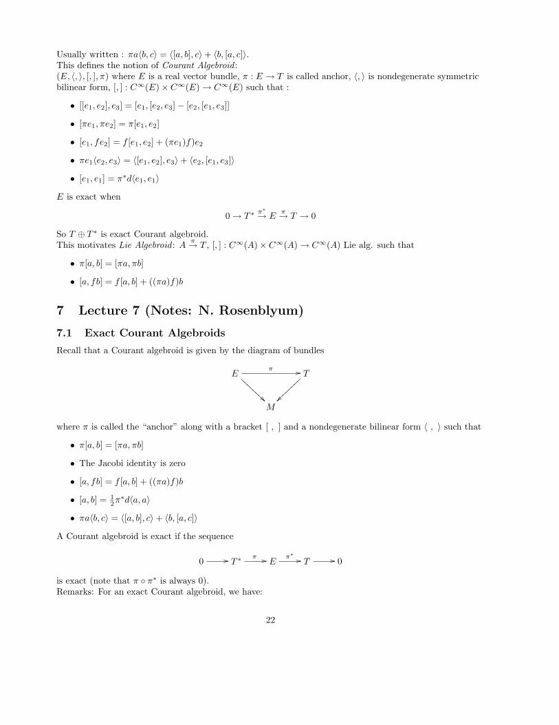
Recall that a Courant algebroid is given by the diagram of bundles

E π �� T

M

where π is called the “anchor” along with a bracket [ , ] and a nondegenerate bilinear form � , � such that

• π[a, b] = [πa, πb]

• The Jacobi identity is zero

• [a, fb] = f [a, b] + ((πa)f)b

[a, b] = 1 π∗d�a, a�• 2

• πa�b, c� = �[a, b], c� + �b, [a, c]�

A Courant algebroid is exact if the sequence

0 �� T ∗ π �� E π∗ �� T �� 0

is exact (note that π π∗ is always 0).◦Remarks: For an exact Courant algebroid, we have:

22

1. The inclusion T ∗ ⊂ E is automatically isotropic because for ξ, η ∈ T ∗,

�π∗ξ, π∗η� = ξ(π∗πη) = 0

since �π∗ξ, a� = ξ(πa).

2. The bracket [ , ]|T ∗ = 0: for s, t ∈ C∞(E), f ∈ C∞(M ),

D = π∗d : C∞(M) → C∞(E)

Now,

�[s, Df ], t� = πs�Df, t� − �Df, [s, t]� = πs(πt(f)) − π[s, t](f) = πt(πs(f)) = �D�Df, s�, f�

Thus, [s, Df ] = D�s, Df�. We also have, [Df, s] + [s, Df ] = D�Df, s� and therefore [Df, s] = 0.

We need to show that [fdxi, gdxj ] = 0. But have [dxi, dxj ] = 0 and

[a, fb] = f [a, b] + ((πa)f)b, [ga, b] = g[a, b] − ((πb)g)a + 2�a, b�dg.

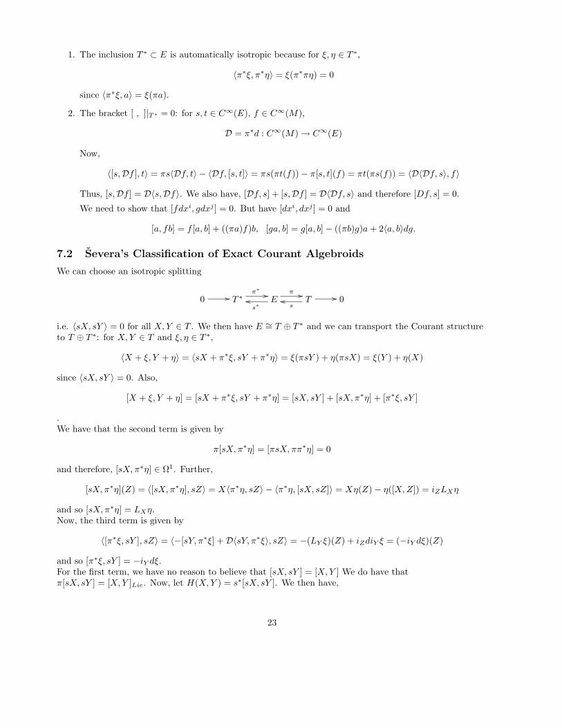
ˇ7.2 Severa’s Classification of Exact Courant Algebroids

We can choose an isotropic splitting

π∗ �� π ��

0 �� T ∗ �� E �� T �� 0 s∗ s

i.e. �sX, sY � = 0 for all X,Y ∈ T . We then have E ∼= T ⊕ T ∗ and we can transport the Courant structure to T ⊕ T ∗: for X,Y ∈ T and ξ, η ∈ T ∗,

�X + ξ, Y + η� = �sX + π∗ξ, sY + π∗η� = ξ(πsY ) + η(πsX) = ξ(Y ) + η(X)

since �sX, sY � = 0. Also,

[X + ξ, Y + η] = [sX + π∗ξ, sY + π∗η] = [sX, sY ] + [sX, π∗η] + [π∗ξ, sY ]

. We have that the second term is given by

π[sX, π∗η] = [πsX, ππ∗η] = 0

and therefore, [sX, π∗η] ∈ Ω1 . Further,

[sX, π∗η](Z) = �[sX, π∗η], sZ� = X�π∗η, sZ� − �π∗η, [sX, sZ]� = Xη(Z) − η([X,Z]) = iZ LX η

and so [sX, π∗η] = LX η. Now, the third term is given by

�[π∗ξ, sY ], sZ� = �−[sY, π∗ξ] + D�sY, π∗ξ�, sZ� = −(LY ξ)(Z) + iZ diY ξ = (−iY dξ)(Z)

and so [π∗ξ, sY ] = −iY dξ. For the first term, we have no reason to believe that [sX, sY ] = [X,Y ] We do have that π[sX, sY ] = [X,Y ]Lie. Now, let H(X,Y ) = s∗[sX, sY ]. We then have,

23

1. H is C∞-linear and skew in X,Y :

H(X, fY ) = fs∗[sX, sY ] + s∗(X(f)sY ) = fs∗[sX, sY ], and

H(fX, Y ) = s∗[fsX, sY ] = fH(X,Y ) − s∗((Y f)sX) + 2�sX, sY �df = fH(X,Y ). Furthermore,

[sX, sY ] + [sY, sX] = π∗d�sX, sY �.

2. H(X,Y )(Z) is totally symmetic in X,Y, Z:

H(X,Y )(Z) = �[sX, sY ], sZ�E = X�sY, sZ� − �sY, [sX, sZ]�

So, we have [sX, sY ] = [X,Y ] − iY iX H for H ∈ Ω3(M).

Problem. Show that [[a, b], c] = [a, [b, c]] − [b, [a, c]] + iπciπbiπadH and so Jac = 0 if and only if dH = 0.

Thus, we have that the only parameter specifying the Courant bracket is a closed three form H ∈ Ω3(M).We will see that when [H]/2π ∈ H3(M, Z), E is associated to an S1-gerbe.Now, let’s consider how H changes when we change the splitting. Suppose that we have two sections1, s2 : T → E. We then have that π(s1 − s2) = 0. So consider B = s1 − s2 : T → T ∗. In the s1 splitting,we have for x ∈ T , s2(x) = (x + (s2 − s1)x). Since the si are isotropic splittings, we have that(s2 − s1)(x)(x) = 0. Thus we have, B ∈ C∞(Λ2T ∗).Now, in the s1 splitting we have,

[X +ixB, Y +iY B]H = [X,Y ]+LX iY B −iY diX B+iY iX H = [X,Y ]+i[X,Y ]B −iY LX B +iY diX B +iY iX H =

= [X,Y ] + i[X,Y ]B + iY iX (H + dB)

In particular, in the s2 splitting H changes by dB. Thus, we have that [H] ∈ H3(M, R) classifies the exact Courant algebroid up to isomorphis. The above bracket is also a derived bracket. Before, we had that

[a, b] ϕ = [[d, a], b]ϕ.C ·

Now, replace d with dH We clearly have that d2 = (dH)∧ = 0 since dH = 0. Note that dH is= d + H∧. H not of degree one and is not a derivation but it is odd. The cohomology of dH is called H-twisted deRham cohomology. In simple cases (e.g. when M is formal in the sense of rational homotopy theory,), we have

H∗(Hev/od(M), e[H]) = Hev/od(M)dH

where eH = H∧.Now, [a, b]H ϕ = [[dH , a], b]ϕ. Indeed, for B ∈ Ω2, we have ϕ �→ eB ϕ and· e−B (d + H∧)eB = e−B deB + e−B HeB = dH+dB , and so eB [e−B , eB ]H = [ , ]H+dB In particular, if· ·B ∈ Ω2

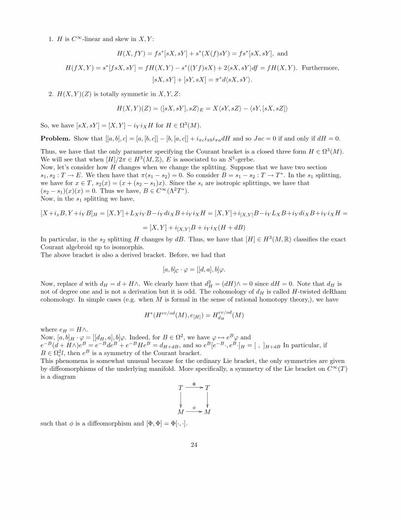
c l, then eB is a symmetry of the Courant bracket.This phenomena is somewhat unusual because for the ordinary Lie bracket, the only symmetries are givenby diffeomorphisms of the underlying manifold. More specifically, a symmetry of the Lie bracket on C∞(T )is a diagram

Φ T �� T

�� φ ��M �� M

such that φ is a diffeomorphism and [Φ, Φ] = Φ[·, ].·

24

� �

Claim 1. Sym[ , ]Lie = {(φ∗, φ), φ ∈ Diff(M)}.

Proof. Given (Φ, φ) ∈ Sym[ , ]Lie, consider G : Φφ−1 . Then G covers the identity map on M and we have∗ fG[X,Y ] − ((Y f)GX = G[fX, Y ] = f [GX,GY ] − (GY )fGX and so Y f = (GY )(f) for all Y, f and so G = 1.

Let’s now consider the question of what all the symmetries of the Courant bracket [ , ] are. Once again,C

we have a diagram

E Φ �� E

�� φ ��M �� M

where E � T ⊕ T ∗ such that

1. φ∗�Φ·, Φ·� = �·, ·�

2. [Φ·, Φ ] = Φ[·, ]· ·

3. π Φ = φ π.◦ ∗ ◦

Suppose that φ ∈ Diff(M). Then on T ⊕ T ∗, φ is given by∗

φ = φ∗

∗ (φ∗)−1

and so we have φ (X + ξ) = φ∗X + (φ∗)−1ξ and∗

φ−1[φ∗X + (φ∗)−1ξ, φ∗Y + (φ∗)−1η]H = [X + ξ, Y + η]φ∗H∗

since φ−1(iφ∗Y iφ∗X H)(Z) = iφ∗Z iφ∗Y iφ∗ X H = φ∗H(X,Y, Z). In particular, this does not give a symmetry∗ unless φ∗H = H.Now, consider a B-field transform. Since eB [e−B , e−B ]H = [·, ]H+dB , this is not a symmetry unless· · ·dB = 0. Now we can combine these to generate the symmetries:

[φ∗e B , φ∗e B ] = φ∗e

B [·, ]φ∗H+dB· · ·

and so φ B ∈ SymE iff H − φ∗H = dB. It turns out that these are all the symmetries.∗e

Theorem 5. The above are all the symmetries of an exact Courant algebroid. In particular, we have a short exact sequence

0 → Ωcl 2 → Sym(E) → Diff[H] → 0

where Diff[H] is the subgroup of diffeomorphisms of M preserving the cohomology class [H].

8 Lecture 8 (Notes: J. Bernstein)

8.1 Dirac Structures

So far we understand the exact Courant Algebroids

0 T ∗ E T 0→ → → →

Which are classified up to isomorphism by [H] ∈ H3(M, R3) and upon a choice of splitting is isomorphic to (T ⊕ T ∗, <,>, [, ]H , π : E → T ). For H ∈ Ω3 Always consider (M,E) or (M,H). Geometry in exactcl. Courant Algebroids consists of studying special subbundles L ⊆ E.

25

Theorem 6. Suppose that L ⊆ E a subbundle which is closed under [, ] (involutive), i.e. [C∞(L), C∞(L)] ⊆ C∞(L). then L must be isotropic or L = π−1(Δ) for Δ ⊆ T integrable distribution. Note, for Δk ⊆ T , π−1(δ) is of dimension n + k and contains T ∗ (so is not isotropic).

Proof. Suppose L is involutive, but not isotropic, then there exists v ∈ C∞(L) with < v, v >m= 0. Now �recall property [fv, v] = f [v, v] − (π(v)f)v + 2 < v, v > df ⇒ 2 < v, v > df ∈ C∞(L) for all f , as [fv, v], f [v, v] ∈ C∞(L). This implies that dfm for all m which tells us that T ∗ but T ∗ is∈ Lm m ⊆ Lm

isotropic so Lm = π−1(Δm) for Δ = 0. Thus rk� L > n evertywhere and so L not isotropic at all points p ∈ M thus Tp

∗ ⊆ Lp for all p and so L = π−1(Δ) where Δ is an integrable distribution.

So interesting involutive subbundles are isotropic subbundles L ⊆ E. Recall that the axioms of a Courant Algebroid imply that [a, a] = 12 π

∗d < a, a >. Thus on L, [, ]C |C∞(L) defines a Lie Algebroid when L is involutive and isotropic. So L ⊆ E with [L,L] ⊆ L and < L,L >= 0 implies that (L, [, ], π) is a Lie Algebroid which implies (C∞(∧∗L∗), dL) gives rise the HdL (M) the Lie Algebroid Cohomology.

Definition 14. When an isotropic, involutive L ⊂ E is maximal it is called a Dirac Structure

Examples of Dirac structures in 0 → T ∗ → E → T → 0

• T ∗ ⊂ E as [T ∗, T ∗] ⊆ [T ∗, T ∗]

• If we split (T ⊕ T ∗, [, ]H ) then [X,Y ]H ∈ C∞(T ) if and only if H = 0 so T ∈ T ⊕ T ∗ is a Diracstructure if and only if H = 0

• Any maximal isotropic transverse L (that is such that L ∩ T ∗ = {0} is of the form L = ΓB . Since eB [e−B , e−B ]H = [·, ]H+dB so eB [T, T ]H−dB = eB [e−BΓB , e

−B ΓB ]H−dB = [ΓB , ΓB ]H . Thus · · ·[ΓB , ΓB ] ⊂ ΓB ] if and only if [T, T ]H−dB ⊆ T and this occurs if and only if H − dB = 0 so ΓB is Dirac when and only when [H] = 0. In particular when [H] = 0 there is no Dirac complement to � T ∗.

• When Δ ⊂ T is an integral distribution then f : Δ ⊕ Ann Δ �→ T ⊕ T ∗ is involutive for [, ]H when and only when f∗H = 0.

• For (T ⊕ T ∗, [, ]H ) and β ∈ ∧2T we consider Γβ . This is Dirac if and only if [β, β] = −β∗H where we think of β : T ∗ → T .

Problem. Verify the condition for Γβ to be Dirac by first showing that [ξ + β(ξ), η + β(η)] = ζ + β(ζ) ifand only if < [ξ + β(ξ), η + β(η)], ζ + β(ζ) >= 0. And then showing that< [df + β(df), dg + β(dg)], dh + β(dh) >= {f, {g, h}} + {g, {h, f}} + {h, {f, g}} + H(β(df), β(dg), β(dh)) =(Jac{, } + β∗H)(df, dg, dh).

Definition 15. if [β, β] = −β∗H then β is called a twisted Poisson Structure.

Suppose that β is a twisted Poisson structure, then eB Γβ is not necessarily Γβ� , in particular if β is invertible (as a map T ∗ → T ) and β−1 = B then e−B Γβ = T . However if B is “small enough” then eB Γβ = Γβ� . To quantify this we note that eB : ξ + β(ξ) �→ β(ξ) + ξ + Bβ(ξ) which we want equal to η + β�(η). This happens if and only if η = (1 + Bβ)ξ and also β(ξ) = β�(η) = β�(1 + Bβ)ξ. Thus β� = β(1 + Bβ)−1 and so smallness just means that the map is invertible (i.e. what is written makes sense).

Definition 16. The transformation from β �→ β(1 + Bβ)−1 is called a gauge transform of β.

Problem. (Severa-Weinstein) Show that if β is Poisson and dβ = 0 then β� is Poisson. Also show that H · = H · (M ), (i.e. one has a isomorphsm of Poisson cohomology. (Hint: eB : Γβ → is an β (M) ∼ β� Γβ�

isomorphism of Lie Algebras).

26

� �

� �

8.2 Geometry of Lie Groups

Recall that for a Lie group G one has a natural action of G × G on G, given by (g, h) x = gxh = Lg Rhx· (here one has a left action and a right action). These actions commute in that (gx)h = g(xh). Now for g = Te

RG the lie algebra of G

L one has two identifications of g → TgG namely a �→ aL|g = (Lg)∗a and

a �→ a |g = (Rg)∗a where a , aR are left and right invariant vector fields respectively. We have by definition [aL, bL]Lie = [a, b]L . Now if j : G → G is given by x �→ x−1, then jLg = Rg−1 j so j (Lg ) = (Rg−1 ) In particular since (j )e = −Id, one has ∗ ∗ ∗j∗. ∗(j∗aL)g−1 = j∗(Lg )∗a = (Rg−1 )∗j∗a = −(Rg−1 )∗a = −aR|g−1 . Thus j∗aL = −aR . Thus [aR, bR] = [j L, j∗b

L] = j [aL, bL] = j [a, b]L = −[a, b]R . One also has [aL, bR] = 0. To see this we note ∗a ∗ ∗that the map g → C∞(TG) given by a �→ aL| = d (gγ(t)) exponentiates to a right action Rγ(t) similarly g dt aR exponentiates to a left action and so [aL, bR] = 0. We now define Adg : g → g by Adg (X) = (Rg−1 )∗(Lg)∗. Equivalently aR|g = (Adg−1 a)L|g . We define adX = d(Adg)0 = [X, ].·

Lemma 1. If ρ ∈ Ωk(G) is bi-invariant then dρ = 0

Proof. If ρ is left invariant then ρ ∈ ∧kg∗ and so

dρ(X0, . . . , Xk) = (−1)iXiρ(X0, . . . , Xi, . . . , Xk) + (−1)i+j ρ([Xi, Xj ], X0, . . . , Xk) i i,j

, where we have chosen X0, . . . Xk�to be left invariant so the first sum is zero . On the other hand right invariance tells us that for all X, ρ(X1, . . . , [X,Xi], . . . , Xk) = 0.

Problem. Show how the statement above implies that dρ = 0.

We define Cartan one-forms to be forms θL, θR ∈ Ω1(G, g) by θgL(v) = (Lg−1 )∗v ∈ g. and

θR(v) = (Rg−1 ) So θL = θL . Thus θL is left invariant as θR is right invariant. g ∗v ∈ g. x ◦ (Lg−1 )∗ gx

For G = Gln, g = Mn one has θL = g−1dg and θR = dgg−1 . Now if g = [gij ] that is gij are coordinates one gets matrix of oneforms [gij ]−1[dgij ]. Then (σg)−1d(σg) = g−1σ−1σdg = g−1dg, and so it is left invariant (similarly one can check that the obvious definition is indeed right invariant). At 1 ∈ GLn one has g consisting of n × n matrices {[aij ]} here we make think of [aij] = i,j aij ∂g

∂ ij

. so

g−1dg( i,j aij ∂g∂

ij ) = aij, so g−1dg|e = Id : g → g. This is also true for θL and θR .


Last time, we talked about the geometry of a connected lie group G. Specifically, for any a in the corresponding Lie algebra g, one can define aL|g = Lg∗a and choose θL ∈ Ω1(G, g) s.t. θL(aL) = a. For instance, for GLn, with coordinates g = [gij ], one has θL = g−1dg, and similarly θR = dgg−1.This implies that dg ∧ θL + gdθL = 0 = dθL + θL ∧ θL = 0 = dθL + 1 [θL, θL] = 0, the latter of which is the Maurer-Cartan equation.

⇒ ⇒ 2

Problem. 1. Extend this proof so that it works in the general case.

2. Show j∗θR = −θL .

3. Show dθR − 1 [θR, θR] = 0. 2

4. Show θR(aL)|g = Ad ga∀a ∈ g, g ∈ G.

27

� � � �

9.1 Bilinar forms on groups

Let G be a connected real Lie group, B a symmetric nondegenerate bilinear form on g. This extends to a left-invariant metric on G, and B is invariant under right translation ⇔ B([X,Y ], Z) + B(Y, [X,Z]) = 0∀X,Y, Z. If this is true, we obtain a bi-invariant (pseudo-Riemannian) metric on G.

Remark. Geodesics through e are one-parameter subgroups B is bi-invariant. See Helgason for Riemannian geometry of Lie groups and homogeneous spaces.

⇔

Example. Let B be the Killing form on a semisimple Lie group, i.e. B(a, b) = Trg(adaadb) for s|m, s m, spm a constant multiple of Tr(X,Y ). Now, we can form the Cartan 3-form◦

1 1 H = B(θL , [θL, θL]) = B(θR , [θR, θR]) (7)

12 12

This H is bi-invariant, and thus closed. When G is simple, compact, and simply connected, the Killing form gives λ[H] as a generator for H3(G, Z) = Z. (See Brylinski.) For instance, given g = s n, θ

L = g−1dg, one has H = Tr(θL ∧ θL ∧ θL) i.e. H = Tr(g−1dg)3 .

|

9.1.1 Key calculation

Let m, p1, p2 : G × G → G be the multiplication and projection maps respectively. Then

m∗H = Tr((gh)−1d(gh))3 = Tr(h−1 g−1(gdh + dgh))3

(8) = Tr(h−1gh)3 + Tr(g−1dg)3 + Tr((dhh−1)2 g−1dg) + Tr(dhh−1(g−1dg)2)

Now, define θ = dhh−1 , Ω = g−1dg, so dθ = θ ∧ θ and dΩ = −Ω ∧ Ω. Then

dTr(dhh−1 g−1dg) = dTr(θ ∧ Ω) = Tr(dθ ∧ Ω − θ ∧ dΩ) (9)

= Tr(θ ∧ θ ∧ Ω + θ ∧ Ω ∧ Ω)

So, m∗H − p1∗H − p∗

2H = dτ , where τ = Tr(dhh−1g−1dg) = B(p∗ 1θ

L, p2∗θR) ∈ Ω2(G × G).

Now, recall that given a metric g : V → V ∗, we have a decomposition V ⊕ V ∗ = C+ ⊕ C− for C± = Γ±.Moreover, any Dirac structure L ⊂ V ⊕ V ∗ can be written as the graph of A ∈ O(V, g) thought of asA : C+ → C−. NOw, for X ∈ V , let X± = X ± gX ∈ C±. Then LA = {X+ ± (AX)− X ∈ V } are the± |Dirac structures. Note that

�X+ ± (AX)−, X+ ± (AX)−� = g(X,X) − g(AX,AX) = 0 (10)

Let B be a bi-invariant metric on G. Then the map Ax = Lx−1∗Rx∗ : TxG → TxG, aL �→ aR is orthogonal

for B and ad(G)-invariant, since

TxG Ax �� TxG

adg∗ (11)adg∗

A gxg−1

Tgxg−1 G �� Tgxg−1 G

where adg∗ = Lg∗Rg−1∗. Thus, we find that

adg∗Axad−1 = LgRg−1 RxLx−1 RgLg−1 = Lg−1x−1gRgxg−1 = Agxg−1 (12)g∗

Overall, L (A) are ad(G)-invariant almost Dirac structures in (T ⊕ T ∗)(G). TxG is spanned by the aL, so±r LL+ is spanned by (aL)+ + (aL)− = aL + B(aL) + a − B(aR) and L+ = �aL + aR + B(a − aR)�. Recall

that θL(aL) = a so �aL + aR + B(aL − aR)� = �aL + aR + B(θL − θR, a)�. Similarly,L− = �aL − aR + B(θL + θR, a)�.

28

Remark. Since aL − aR generates the adjoint action, [aL − aR, bL − bR] = [a, b]L − [a, b]R . But [aL + aR, bL + bR] = [a, b]L + [a, b]R is not integrable. L (A) is integrable, however, w.r.t. the Courant bracket twisted by H = B(θL , [θL, θL]).

−


Last time, we defined an almost Dirac structure on any Lie group G with a bi-invariant metric B by

LC L R + B(a L + a R) (13)= �a − a |a ∈ g�

10.1 Integrability

Lemma 2. d(B(aL))(xL, yL) = xLB(aL, yL) − yLB(aL, xL) − B(aL , [xL, yL]) = −iaL H(xL, yL), whereH(a, b, c) = B(aL , [bL, cL]).

Problem. Show that B(θL , [θL, θL])(aL, bL, cL) = 6B(aL , [bL, cL]).

Note also that

dB(a R)(x R , y R) = −B(a R , [x R , y R]) = iaR H(x R , y R) (14)

Now,

[a L − a R + B(a L + a R), bL − bR + B(bL + bR)]0 = [a, b]L − [a, b]R − ibL−bR dB(a L + a R) + La −aR B(bL + bR)L

= [a, b]L − [a, b]R + ibL−bR ia −aR H + B([a, b]L + [a, b]R)L

(15)

Corollary 3. LC is involutive under [, ]H .

Comments about the Cartan-Dirac structure:

1. aL − aR generates the adjoint action so generalized, and πLC = Δ is a foliation by the conjugacyclasses.

2. T ∗ component is B(aL + aR), which spans T ∗ whenever g → Tg ∗, a �→ aL + aR is surjective ⇔ (adg + 1

is invertible. This is true, in particular, for an open set containing e ∈ G.

In this region, Lc = Γβ for an H-twisted Poisson structure.

1. Determine explicitly the bivector β when it is defined.

2. For G = SU(2) = S3, describe the conjugacy classes and the locus where adg + 1 is invertible, rank 2, rank 1, and rank 0.

3. Determine the Lie algebroid cohomology H∗(Lc). Hint: g → Lc, a �→ aL − aR + B(aL + aR) isbracket-preserving.

10.2 Dirac Maps

A linear map f : V W of vector spaces induces a map f : Dir(V ) Dir(W ) (the forward Dirac map) → ∗ →given by f∗LV = {f∗v + η ∈ W ⊕ W ∗ v + f∗η ∈ LV } and a map f∗ : Dir(W ) Dir(V ) (the backward Dirac map) given by f∗LW f= {v + f∗

|η ∈ V ⊕ V ∗| ∗v + η ∈ LW }.

→

29

� � � �

Example.

β ∈ �2

V . Then

f∗Γβ = {f∗v + η|v + f∗η = β(ξ) + ξ∀ξ ∈ V ∗} = {f∗βf∗η + η|η ∈ W ∗} = {(f∗β)(η) + η} = Γf

(16) ∗β

so f coincides with the usual pushforward. ∗

L = L(E, �), f : E � V, � ∈ �2

E∗. Then L is precisely f Γ� via the pushforward E ⊕ E∗ → V ⊕ V ∗.→ �2

∗

In general, L = L(F, γ), F ⊂ V ∗, γ ∈ F ∗ is equivalent to specifying(C = Ann F = L ∩ V, γι

�2 F ∗ =

�2(V/L ∩ V ) = �2(V/C)). Note that (f∗LV ) ∩ W = f (LV ∩ V ).∗

Problem. f∗L(C, γ) = L(f∗C, f∗γ).

This proves that pushforward commutes properly with composition.

10.3 Manifolds with Courant Structure

Let (M,HM ), (N,HN ) be manifolds equipped with H ∈ Ω3)cl-structure.

Definition 17. A morphism Φ : (M,HM ) (N,HN ) is a pair (φ,B) for φ : M N a smooth map and→ →B ∈ Ω2(M) s.t. φ∗HN − HM = dB, i.e. B gives an isomorphism φ∗GN → GM .

Now, suppose that LM ⊂ TM ⊕ T ∗M,LN ⊂ TN ⊕ T ∗N are Dirac structures.

Definition 18. Φ is a Dirac morphism ⇔ φ∗eB LM = LN .

If LM is transverse to T ∗M , then a Dirac morphism to (N,HN , LN ) is called a Dirac brane for N : thisobject is important because φ∗GN is trivial.

Example. Let LN be a Dirac structure, and let M ⊂ N be a leaf of Δ = πLN . ThenLN = L(Δ, � ∈

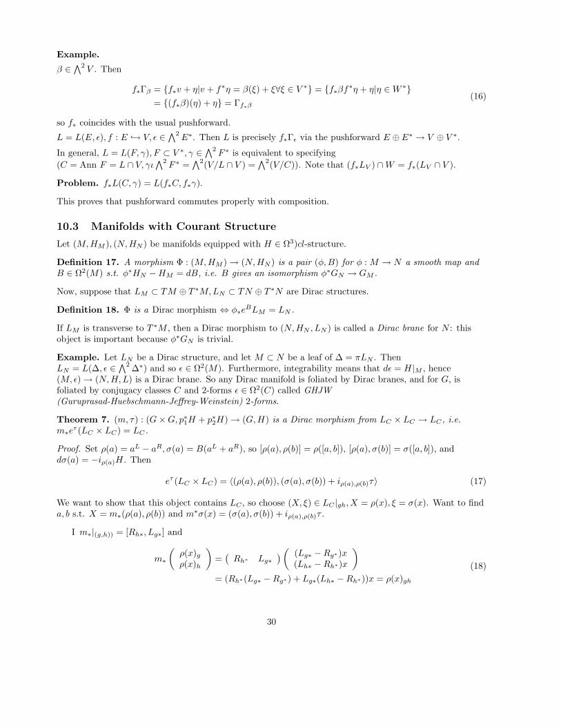
�2 Δ∗) and so � ∈ Ω2(M). Furthermore, integrability means that d� = H|M , hence(M, �) (N,H,L) is a Dirac brane. So any Dirac manifold is foliated by Dirac branes, and for G, is→foliated by conjugacy classes C and 2-forms � ∈ Ω2(C) called GHJW (Guruprasad-Huebschmann-Jeffrey-Weinstein) 2-forms.

Theorem 7. (m, τ ) : (G × G, p∗ 1H + p∗

2H) (G,H) is a Dirac morphism from LC × LC → LC , i.e. m τ (LC × LC ) = LC .

→ ∗e

Proof. Set ρ(a) = aL − aR, σ(a) = B(aL + aR), so [ρ(a), ρ(b)] = ρ([a, b]), [ρ(a), σ(b)] = σ([a, b]), and dσ(a) = −iρ(a)H. Then

e τ (LC × LC ) = �(ρ(a), ρ(b)), (σ(a), σ(b)) + iρ(a),ρ(b)τ� (17)

We want to show that this object contains LC , so choose (X, ξ) ∈ LC |gh, X = ρ(x), ξ = σ(x). Want to find a, b s.t. X = m (ρ(a), ρ(b)) and m∗σ(x) = (σ(a), σ(b)) + iρ(a),ρ(b)τ .∗

I m∗|(g,h)) = [Rh∗, Lg∗] and

ρ(x)g � � (Lg∗ − Rg∗ )x m = Rh∗ Lg∗∗ ρ(x)h (Lh∗ − Rh∗ )x (18)

= (Rh∗ (Lg∗ − Rg∗ ) + Lg∗(Lh∗ − Rh∗ ))x = ρ(x)gh

30

� �

� �

�

II Want to show m∗σ(x)gh = (σ(a)g , σ(b)h) + iρ(a)g ,ρ(b)h τ . At gh, we have that

R m∗σ(x)

abL = σ(x)(Rh∗a R + Lg∗b

L) = σ(x)(a R + bL) = B(x L − x R , a R + bL) (19)

Then

R (σ(x), σ(x))

abL = σ(x)g(a R) + σ(x)h(bL) (20)

and the rest follows.

This leads to a fusion operation on Dirac morphisms: given Φ1 : M1 → G, Φ2 : M2 → G, composing the product with (m, τ) gives Φ1 � Φ2 : M1 × M2 → G.

Example. Given two copies of the map m : G × G → G, obtain m � m : G4 → G: more generally, get Dirac morphisms M�h : G2h G. This is used by AMM to get a symplectic structure on the moduli space →of flat G-connections on a genus h Riemann surface.

By Freed-Hopkins, fusion on branes implies a form of fusion on Kτ (G).G

11 Lecture 11(Notes: K. Venkatram)

11.1 Integrability and spinors

Given L ⊂ T ⊕ T ∗ maximal isotropic, we get a filtration 0 ⊂ KL = F 0 ⊂ F 1 = Ω∗(M) via �k+1 ⊂ · · · ⊂ F n

F k = {ψ : L ψ = 0}. Furthermore, for φ ∈ KL, we have ·

X1X2dφ = [[d,X1], X2]φ = [X1, X2]φ (21)

for all X1, X2 ∈ L (where d = dH ). Thus, in general, dφ ∈ F 3, and L is involutive ⇔ dφ ∈ F 1 . Now, assume d(F i) ⊂ F i+3 (and in F i+1 if L is integrable) ∀i < k and ψ ∈ F k . Then

[X1, X2]ψ = [[d,X1], X2]ψ = dX1X2ψ + X1dX2ψ − X2dX1ψ − X2X1dψ (22)

X1X2dψ = −dX1X2ψ − X1dX2ψ + X2dX1ψ + [X1, X2]ψ

Note that, in the latter expression, each of the parts on the RHS have degree (k − 1) + 2 = k + 1, sodψ ∈ F k+1 if L is integrable and F k+3 otherwise.Next, suppose that the Courant algebroid E has a decomposition L ⊕ L� into transverse Dirac structures.

1. Linear algebra:

= L∗ via �·, ·�.• L� ∼

The filtration KL = F 0 ⊂ F 1 of spinors becomes a Z-grading• �k ⊂ · · · ⊂ F n � �k

KL ⊕ (L� · KL) ⊕ · · · ⊕ ( L� · KL) ⊕ · · · ⊕ (det L� · KL), i.e. ( L∗)KL.

Remark. Note that L� · (det L� · KL) = 0, so det L� · KL = det L∗ ⊗ KL = KL� .

Thus, we have a Z grading S = nk=0 Uk.

• If the Mukai pairing is nondegenerate on pure spinors, then KL ⊗ KL� = det T ∗.

31

2. Differential structure: via the above grading, we have F k(L) = �

ik =0 Ui, F k(L�) =

�ik =0 Un−i, so

d(Uk) = d(F k(L) ∩ F n−k(L�). By parity, dUk ∩ Uk = 0, so a priori

d = (πk−3 + πk−1 + πk+1 + πk+3) ◦ d = T � + ∂� + ∂ + T (23)

Problem. Show that T � : Uk → Uk−3, T : Uk → Uk+3 are given by the Clifford action of tensors �3 �3T � ∈ L, T ∈ L∗.

Remark. This splitting of d = dH can be used to understand the splitting of the Courant structure on L ⊕ L∗. Specifically, d2 = 0 = ⇒

−4 T �∂� + ∂�T � = 0 −2 (∂�)2 + T �∂ + ∂T �

0 ∂∂� + ∂�∂ + TT � + T �T (24) 2 ∂2 + T∂� + ∂�T 4 T∂ + ∂T = 0

11.2 Lie Bialgebroids and deformations

We can express the whole Courant structure in terms of (L,L∗). Assume for simplicity that L,L∗ are both integrable, so T = T � = 0. Then

1. Anchor π → a pair of anchors π : L → T, π� : L� → T .

2. An inner product → a pairing L� = L∗, �X + ξ,X + ξ� = ξ(X).

3. A bracket → a bracket [, ] on L, [, ]∗ on L∗. Specifically, for x, y ∈ L, φ ∈ U0,

[x, y]φ = [[d, x], y]φ = xydφ = xy(∂ + T )φ = xyTφ = (ixiy T )φ (25)

The induced action on S is dLα = [∂, α], giving us an action of L on L∗ as πL∗ [x, ξ] for x ∈ L, ξ ∈ L∗. Expanding, we have

[x, ξ]φ = [[∂, x], ξ]φ = ∂xξφ + x∂ξφ − ξx∂φ − (ixξ)∂φ (26)

= ∂(ixξ)φ + x(dLξ)φ − (ixξ)∂φ = (dLixξ + ixdLξ)φ = (Lxξ)φ

If T = 0, then x Lx is an action (guaranteed by the Jacobi identity of the Courant algebroid). If L,L�

are integrable, →

Lx[ξ, η] = πL∗ [x, [ξ, η]] = πL∗ ([[x, ξ], η] + [ξ, [x, η]]) (27)∗

Problem. This implies that d[·, ·]∗ = [d·, ·]∗ + [·, d·]∗.

As a result of these computations, we find that, for X,Y ∈ L, ξ, η ∈ L∗,

[X + ξ, Y + η] = [X,Y ] + [X, η]L + [ξ, Y ]L + [ξ, η] + [ξ, Y ]L∗ + [X, η]L∗

= [X,Y ] + Lξ Y − iη d∗X + [ξ, η] + LX η − iY dξ (28)

There are no H terms since we assumed T = T � = 0. Overall, we have obtained a correspondence between transverse Dirac structures (L,L�) and Lie bialgebroids (L,L∗) with actions and brackets L T,L∗ → T s.t. d is a derivation of [, ]∗.

→

32

� �

� �

Finally, we can deform the Dirac structure in pairs. Specifically, for � ∈ C∞( �2

L∗) a small B-transform, e�(L) = L�, one can ask when L� is integrable. We claim that this happens dL� + 1 [�, �] = 0. To see ⇔ 2 ∗

this, note that

�[e � x, e � y], e � z� = �[e � x, e � y]L, e � z� + �[e � x, e � y]L∗ , e � z�1 (29)

= (dL�)(x, y, z) + [�, �] (x, y, z)2 ∗

via an analogous computation to that of eB T and eπT ∗ from before.

12 Lecture 12-17(Notes: K. Venkatram)

12.1 Generalized Complex Structures and Topological Obstructions

Let E ∼= (T ⊕ T ∗,H) be an exact Courant algebroid.

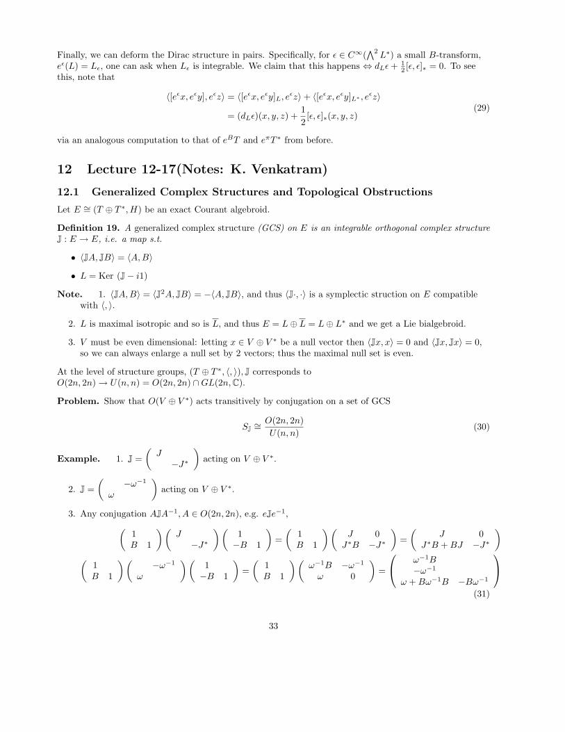
Definition 19. A generalized complex structure (GCS) on E is an integrable orthogonal complex structure J : E E, i.e. a map s.t. →

• �JA, JB� = �A,B�

• L = Ker (J − i1)

Note. 1. �JA,B� = �J2A, JB� = −�A, JB�, and thus �J·, ·� is a symplectic struction on E compatible with �, �.

2. L is maximal isotropic and so is L, and thus E = L ⊕ L = L ⊕ L∗ and we get a Lie bialgebroid.

3. V must be even dimensional: letting x ∈ V ⊕ V ∗ be a null vector then �Jx, x� = 0 and �Jx, Jx� = 0, so we can always enlarge a null set by 2 vectors; thus the maximal null set is even.

At the level of structure groups, (T ⊕ T ∗, �, �), J corresponds to O(2n, 2n) → U(n, n) = O(2n, 2n) ∩ GL(2n, C).

Problem. Show that O(V ⊕ V ∗) acts transitively by conjugation on a set of GCS

O(2n, 2n)= (30)SJ ∼

U(n, n)

Example. 1. J = J −J∗ acting on V ⊕ V ∗.

2. J = −ω−1

acting on V ⊕ V ∗. ω

3. Any conjugation AJA−1, A ∈ O(2n, 2n), e.g. eJe−1 , � �� 1 J 1 1 J 0 J 0

= = B 1 −J∗ −B 1 B 1 J∗B −J∗ J∗B + BJ −J∗ ⎛ ⎞ � �� ω−1B ⎝ ⎠

B 1

1 ω −ω−1 1

1 = B 1

1 ω−

ω

1B −ω0

−1 = −ω−1

−Bω + Bω−1B −Bω−1

(31)

33

Lemma 3. O(n.n) � O(n) × O(n).

Proof. Let C+ ⊂ V ⊕ V ∗ be positive definite and C = C⊥. THen O(n, n) acts transitively on the space of− +

all C+, with stabilizer Stab(C+) = O(n) × O(n). Question: what is O(n,n) ? C � (see diagram below) is O(n)×O(n) +

given by A : Rn Rn , ||Ax|| < ||x||∀x, i.e. ||A||op < 1. Thus, it is the unit ball under the operator → norm.

Lemma 4. U(n, n) � U(n) × U(n)

Proof. We can enlarge C+ to C+ by adding V ⊥ C+ and JV , and get complex decompositionE = C+ ⊕ C⊥ = C+ + C−. U(n, n) acts transitively on these spaces with stabilizer + Stab(C+) = U(n) × U(n). As above, we obtain the unit ball in Cn .

Thus, the existence of J is topologically equivalent to the reduction to U(n) × U(n), i.e. complex structures J± := J| ± on C+ and C− = C⊥ (since the bundle of positive-definite subspaces is contractible). C +

Note. The projection π : C T is an isomorphism, so we obtain almost complex structure J : T T .± → ± →

Thus M must be almost complex, and J has two sets of Chern classes c±i ∈ H2i(M, Z) associated to J±(i.e. c±i = ci(c±)) and c(T ⊕ T ∗, J) = c(C+) ∪ c(C−).

Remark. Topologically, E has structure group U(n, n) � U(n) × U(n), so the bundle is classified by ψ : X → B(U(n) × U(n)) = BU(n) × BU(n) = C+ × C− with Chern classes ψ∗C+, ψ∗C−.

Now, spaces L ⊂ T ⊕ T ∗ correspond to canonical bundes KL ⊂ Ω∗(M).

Proposition 5. A generalized complex structure is equivalent to a complex Dirac structure of real index 0, i.e. to a Dirac structure L ⊂ (T ⊕ T ∗) ⊗ C s.t. L ∩ L = {0}.

Proof. ⇐: given L, set J = i|L + (−i)| , and obtain L

�J(α + β), J(α + β)� = �iα − iβ, iα − iβ� = �α, β� + �β, α� = �α + β, α + β� (32)

→: given J, set L = Ker (J − i1), so

�α, β� = �Jα, Jβ� = −�α, β� = 0 (33)

Therefore, (T ⊕ T ∗) ⊗ C = L ⊕ L, and we obtain a transverse complex Dirac structure. This gives us a Z-grading on S ⊗ C = Ω∗(M, C) as

(KL = Un) ⊕ Un−1 ⊕ · · · ⊕ U−n+1 ⊕ (U−n = KL) (34)

with conjugation exchanging Uk and U−k.

Definition 20. KL = U−n is the canonical line bundle of the generalized complex structure.

Furthermore, the decomposition dH = ∂ + ∂ gives the general Dolbeault complex via ∂ : Uk ↔ Uk−1 : ∂.

Problem. Use the Mukai pairing between KL and KL to show that 2c1(KL) = c∗ 1 + c−1 .

34

� � � �

��

� � �

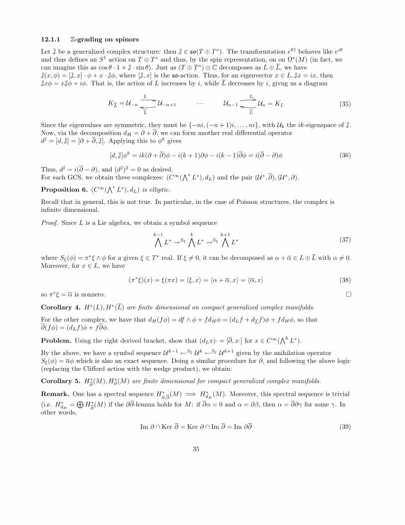
12.1.1 Z-grading on spinors

iθLet J be a generalized complex structure: then J ∈ so(T ⊕ T ∗). The transformtation eθJ behaves like eand thus defines an S1 action on T ⊕ T ∗ and thus, by the spin representation, on on Ω∗(M) (in fact, we can imagine this as cos θ 1 + J sin θ). Just as (T ⊕ T ∗) ⊗ C decomposes as L ⊕ L, we have· · J(x, φ) = [J, x] φ + x Jφ, where [J, x] is the so-action. Thus, for an eigenvector x ∈ L, Jx = ix, then· · Jxφ = xJφ + iφ. That is, the action of L increases by i, while L decreases by i, givng us a diagram

L L

KL = U−n �� U−n+1 · · · Un−1 �� Un = KL (35) L L

Since the eigenvalues are symmetric, they must be {−ni, (−n + 1)i, . . . , ni}, with Uk the ik-eigenspace of J. Now, via the decomposition dH = ∂ + ∂, we can form another real differential operator dJ = [d, J] = [∂ + ∂, J]. Applying this to φk gives

[d, J]φk = ik(∂ + ∂)φ − i(k + 1)∂φ − i(k − 1)∂φ = i(∂ − ∂)φ (36)

Thus, dJ = i(∂ − ∂), and (dJ)2 = 0 as desired. For each GCS, we obtain three complexes: (C∞( ∗

L∗), dL) and the pair (U∗, ∂), (U∗, ∂).

Proposition 6. (C∞( ∗ L∗), dL) is elliptic.

Recall that in general, this is not true. In particular, in the case of Poisson structures, the complex is infinite dimensional.

Proof. Since L is a Lie algebra, we obtain a symbol sequence

k−1 k k+1

L∗ Sξ L∗ Sξ L∗ (37) → →

where Sξ(φ) = π∗ξ ∧ φ for a given ξ ∈ T ∗ real. If ξ = 0, it can be decomposed as� α + α ∈ L ⊕ L with α = 0.�Moreover, for x ∈ L, we have

(π∗ξ)(x) = ξ(πx) = �ξ, x� = �α + α, x� = �α, x� (38)

so π∗ξ = α is nonzero.

Corollary 4. H∗(L),H∗(L) are finite dimensional on compact generalized complex manifolds.

For the other complex, we have that dH (fφ) = df ∧ φ + fdH φ = (dLf + d f)φ + fdH φ, so thatL

∂(fφ) = (dLf)φ + f∂φ.

Problem. Using the right derived bracket, show that (dLx) = [∂, x ] for x ∈ C∞( �k

L∗).· ·

By the above, we have a symbol sequence Uk−1 ← Sξ Uk ← Sξ Uk+1 given by the anihilation operator Sξ(φ) = αφ which is also an exact sequence. Doing a similar procedure for ∂, and following the above logic (replacing the Clifford action with the wedge product), we obtain:

Corollary 5. H∂ ∗(M),H∂

∗(M) are finite dimensional for compact generalized complex manifolds.

Remark. One has a spectral sequence H∗ (M) = H∗ (M). Moreover, this spectral sequence is trivial � ∂,∂ ⇒ dH

(i.e. Hd∗

H = H

∂ ∗(M) if the ∂∂-lemma holds for M : if ∂α = 0 and α = ∂β, then α = ∂∂γ for some γ. In

other words,

Im ∂ ∩ Ker ∂ = Ker ∂ ∩ Im ∂ = Im ∂∂ (39)

35

�

�

��

� � �

��

��

��

��

��

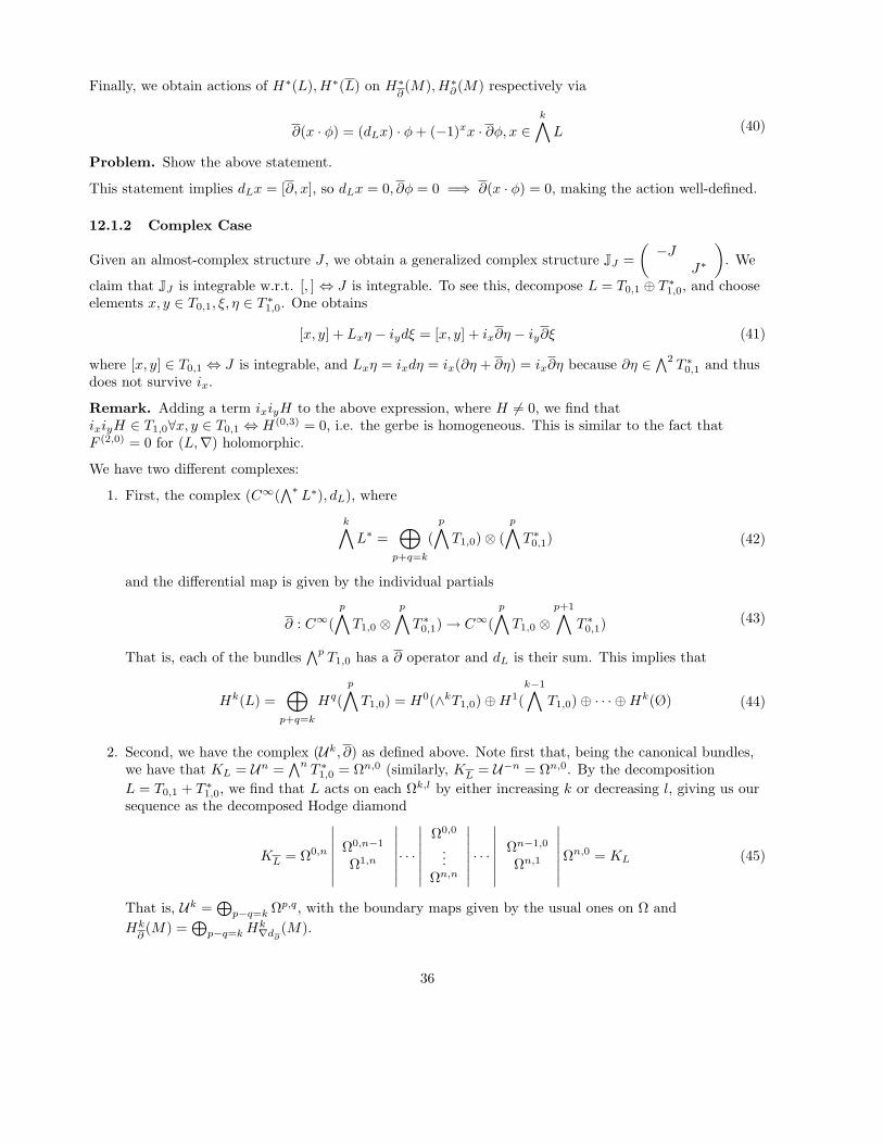
Finally, we obtain actions of H∗(L),H∗(L) on H∂ ∗(M),H∂

∗(M) respectively via

k

∂(x φ) = (dLx) φ + (−1)x x ∂φ, x ∈ L· · ·

Problem. Show the above statement.

(40)

This statement implies dLx = [∂, x], so dLx = 0, ∂φ = 0 = ∂(x φ) = 0, making the action well-defined. ⇒ ·

12.1.2 Complex Case

Given an almost-complex structure J , we obtain a generalized complex structure JJ =

� J−

We J∗ .

claim that JJ is integrable w.r.t. [, ] ⇔ J is integrable. To see this, decompose L = T0,1 ⊕ T1∗ ,0, and choose

elements x, y ∈ T0,1, ξ, η ∈ T1∗ ,0. One obtains

[x, y] + Lxη − iydξ = [x, y] + ix∂η − iy∂ξ (41)

where [x, y] ∈ T0,1 ⇔ J is integrable, and Lxη = ixdη = ix(∂η + ∂η) = ix∂η because ∂η ∈ �2

T ∗ and thus 0,1 does not survive ix.

Remark. Adding a term ixiyH to the above expression, where H = 0, we find that �ixiy H ∈ T1,0∀x, y ∈ T0,1 ⇔ H(0,3) = 0, i.e. the gerbe is homogeneous. This is similar to the fact that F (2,0) = 0 for (L, �) holomorphic.

We have two different complexes:

k� ∗L

∗ L∗), dL), where 1. First, the complex (C∞(

p p� = ( T1,0) ⊗ ( T0

∗ ,1) (42)

p+q=k

and the differential map is given by the individual partials

+1p p p p� ∂ : C∞( T1,0 ⊗ T0

∗ ,1) → C∞( T1,0 ⊗ T0

∗ ,1)

(43)

That is, each of the bundles p T1,0 has a ∂ operator and dL is their sum. This implies that

k 1p −� Hk(L) = Hq( T1,0) = H0(∧kT1,0) ⊕ H1( T1,0) ⊕ · · · ⊕ Hk(Ø) (44)

p+q=k

2. Second, we have the complex (Uk , ∂) as defined above. Note first that, being the canonical bundles, we have that KL

n T1∗ ,0 = Ωn,0 (similarly, KL = U−n = Ωn,0

, we find that L acts on each Ωk,l by either increasing k or decreasing l, giving us our By the decomposition = Un = .

L = T0,1 + T1∗ ,0

sequence as the decomposed Hodge diamond

L = Ω0,n Ω0,n−1

Ω1,n · · · Ω0,0

. . . Ωn,n

· · · Ωn−1,0

Ωn,1 Ωn,0 = KL (45)K

That is, UHk

k = Ωp,q, with the boundary maps given by the usual ones on Ω and p−q=k

Hk ∂ (M) = p−q=k �d∂

(M).

36

� �

� �

� �

� � � �

12.1.3 Symplectic Case

Given a symplectic form ω, we obtain a generalized complex structure Jω = −ω−1

. Given an ω

i-eigenvector x

, we have ξ

ω(x) − ω−1(ξ) = ix + iξ = ⇒ iη = ω(x) (46)

Thus, L = {x − iω(x) : x ∈ T ⊗ C} = Γ−iω, where Γ−iω denotes the graph of −iω : T ⊗ C T ∗ ⊗ C, is a →simple Dirac structure. Moreover, Ωσ is integrable w.r.t. [, ]H dH σ = 0. In our case, we have ⇔d(−ω) = −H ∧ (−iω), so dω and H must be 0 (i.e. ω is symplectic). We again get two complexes

1. (C∞( ∗ L∗)dL) ∼ ∗

T ∗ ⊗ C), d) is trivial, and Hk(L) ∼ (M). However, one does have a = (C∞( = Hk � dR

nontrivial Gerstenhaber structure (C∞( ∗ L∗), dL, [, ] ), and one has an equivalence between (L,L)∗

and (T ⊗ C, Γ(∂iω)−1 ) (the Lie bialgebroid of a complex Poisson structure).

2. The ends of the complex (Uk , ∂) can be simply exhibited as KL = �eiω�,KL = �e−iω�. The next term can be computed via

U−n+1 = (X − iωX)e−iω = −iω(x) ∧ e−iω − iω(x) ∧ e−iω = e iω Ω1 (47)·

2The higher terms are more complicated: given general invertible σ, the transformation e−σe σ−1

on T ⊕ T ∗ sends T ∗ → Γσ (i.e. 1 → eσ) and T → Γ−σ (i.e. Ωn → e−σ). Thus, we find that

Uk = e iω e ω2−i

1

Ωn−k (48)

Letting L, Λ denore the maps φ �→ ω ∧ φ, φ �→= −iω−1 φ, we obtain the expression Uk = eiLe− 2Λ i Ωn−k .

ω−1 These maps arise via the decomposition of J as −ω

+ . Setting

� � � � � �

H = [L, Λ] = 0 0

0 −1

− 1 0

0 0

= 1 0

0 −1

(49)

we find that [H,L] = −2L and [H, Λ] = 2Λ. These are precisely the sl2R commutator relations, giving us associated actions on the symplectic manifold. In particular, H acts as

1 Hφ = tr(id) − (id∗)φ = sum(n − k)πkφ (50)

2

where πk : Ω Ωk is the projection. Via our decomposition of J, we find that →dJ = [d, L + Λ] = [d, Λ] = δ is a degree −1 operator with δ2 = 0 (called the symplectic adjoint of d) and ∂ = d − iδ : Uk → Uk−1 . Using an analogous dδ (or ∂∂) lemma for symplectic manifolds, we find that any cohomology class α ∈ H∗ has a δ-closed representation (since δα = δdγ and d(α − γ) = 0, dR implying that δ(α − dγ) = 0). Thus, setting α = α − γ, we find that

˜ � [d, J]alpha = 0 [d, Λ]α = 0 = d( α) = 0. These statements combine to give an action of (L, Λ)⇔ ⇒

H2n−kon cohomology, i.e. an sl2R action on H∗(M). Furthermore, Ln−k : Hk is an isomorphism, implying an equivalence between the dδ-lemma and the Lefshetz properlty

→(see Cavalcanti thesis for

).⇐

37

� � � �

� �

� �

12.2 Intermediate Cases

We have studied

JJ = J

, Jω = −ω−1

(51)−J∗ ω

What about the intermediate cases?

• intermediate types and spinors

Poisson structure•

Local form •

• Examples of type jumping by deformation

• interpolation

Given a complex bundle T ∗ → E → π T , let J � E with JT ∗ = T ∗. Then T ∗ ⊂ E is a complex subspace, and E/T ∗ = T obtains an almost complex structure J which is integrable. Furthermore,

(Jξ)(X) = �Jξ, X� = −�ξ, Jx� = ξ(Jx) = −J∗ξ(X) (52)

i.e. J|T ∗ = −J∗.

12.2.1 Complex and Symplectic Decompositions

Let S : T → E be any splitting, i.e. π ◦ s = id|T . Then we can produce a complex splitting by averaging

1 2(S − JsJ) = S� (53)

Note. π(−JsJ)(X) = π(−J(s(JX))) = −J2X = X, so −JxJ is a splitting.

JObserve that, in splitting S� : E → T ⊕ T ∗, we obtain J = −J∗ .

Problem. Write J is a non-complex splitting using S. Hint: what is the difference between the splittings S and −JSJ?

Finally, assume that JT ∗ ∩ T ∗ = {0}. Then E = T ∗ ⊕ JT ∗ and, in this splitting,

J = −ω−1

(54)ω

where ω(X,Y ) = �JxX, xY �.

12.2.2 General case

In general, T ∗ + JT ∗ is a complex subspace of E, as is T ∗ ∩ J∗T ∗ ⊂ T ∗ + JT ∗ ⊂ E.

Definition 21. Δ = π(T ∗ + JT ∗) = πJT ∗.

Note that

Ann Δ = (T ∗ + JT ∗)⊥ ∩ T ∗ = T ∗ ∩ JT ∗ ∩ T ∗ = T ∗ ∩ JT ∗ (55)

is complex, and T ∗+JT ∗

= Δ∗ ⊕�J Δ has symplectic structure. Also, E/(T ∗ + JT ∗) = T/Δ has a complex Ann Δ ∼

structure, with complex dimension k (called the type).

38

� �

Theorem 8. M is generally foliated by symplectic leaves with transverse complex structure.

Lemma 5. JT ∗ is Dirac.

Proof. Observe first that the +i eigenspace is closed, i.e.

z − iJz = [x − iJx, y − iJy] = [x, y] − [Jx, Jy] − i([x, Jy] + [Jx, y])

[x, Jy] + [Jx, y] = J[x, y] − J[Jx, Jy] (56)

[Jx, Jy] = [x, y] + J([x, Jy] + [Jx, y])

Thus, [Jξ, Jη] = [ξ, η] + J([ξ, Jη] + [Jξ, η]) = Jα (note that πα = 0 = ⇒ α ∈ T ∗).

Problem. Show that NJ(x, y) = [Jx, Jy] − J[x, Jy] − J[Jx, y] − [x, y] is tensorial and express it in terms of T, T �.

Problem. eθJT ∗ is Dirac ∀θ. Hint: eθJT ∗ = ((cos θ 1) + (sin θ)J)(T ∗) = (1 + tan θJ)T ∗, and ·

[ξ + tJξ, η + tJη] = t([ξ, Jη] + [Jξ, η]) + t2J([ξ, Jη] + [Jξ, η]) = (1 + tJ)(t([ξ, Jη] + [Jξ, η])) (57)

Lemma 6. For small θ, eθJT ∗ is a twisted Poisson structure in a splitting satisfying [π, π] = �3

π∗H. dTaking the derivative (eθJT ∗) at θ = 0, we obtain a tangent vector to Dir(T ⊕ T ∗) at T ∗: this is a skew dθ

map T ∗ T , i.e. an element π ∈ C∞( �2

T ) s.t. [θπ, θπ] = θ3π∗H = [π, π] = 0. Thus, d (eθJT ∗) = π, and π : ξ

→�→ πT Jξ is a Poisson structure, and we can split

⇒ dθ

A πJ = (58)σ −A∗

The proof of the theorem follows from the following two observations:

1. Δ = Im (π) is the image of a Poisson structure and thus a generalized distribution.

2. The symplectic structure on Δ agrees with π, i.e. for ξ, η ∈ Δ∗, ω−1(ξ, η) = �Jξ, η� = π(ξ, η).

12.2.3 Weinstein Splitting

Now, assume that the foliation is of locally constant rank near p ∈ M .

Theorem 9 (Weinstein Splitting). For any p ∈ (M,π) Poisson, there exist coordinates (q1, . . . , qr, p1, . . . , pr, y1, . . . , y�) s.t.

r �� ∂ ∂ � ∂ ∂ π =

∂qi ∧ ∂pi

+ φ(y) ∂yi ∧ ∂yj

(59) i=1 i,j=1

with φ(0) = 0.

Note. • When � = 0, this is the Darboux theorem.

• When the rank at p is locally constant, φ = 0 in a neighborhood of p. (Lie’s Theorem)

If the rank is locally constant, then J induces a complex structure J on �y1, , y2k� which is integrable · · · since (πx, πy) = π(x, y). Moreover, it is independent of the {pi, qi}, as

[Jdpi, Jdyj ] = J(d{pi, yj }) = 0 (60)

and similarly for q. This gives us a local coordinate system R2(n−k) × Ck .

39

� �

� � �

� �

12.2.4 Examples of type jumping

Given a complex structure JJ = −J

and spaces J∗

2 2 2

L = T0,1 ⊕ T1∗ ,0, L∗ = T1,0 ⊕ (T1,0 ⊗ T0

∗ ,1) ⊕ T0

∗ ,1

(61)

we can examine deformations � ∈ �2

L∗ s.t. d� + 1 [�, �] = 0. 2

Example. For � ∈ �2

T1,0,

2 3� � 1 T1,0 ⊗ T0

∗ ,1 ⊕ T1,0 � ∂� +

2[�, �] = 0 = ⇒ ∂� = 0, [�, �] = 0 (62)

i.e. � is a holomorphic Poisson structure.

By construction, � �� 1 � L

= 1 + � + � (63)� 1 L

Letting P = � + �, we obtain a transformation JJ �→ epJe−P , � � � � � � � � � � � � � � 1 P

1 J −J∗

1 −P 1

= 1 P

1 J 0 −JP −J∗ =

J 0 −JP − P J∗

−J∗ = P J 2Q

−J∗

(64)

for Q = i(� − �). Thus, the type is given by n − rkQ.

Example. On CP 2 , �2

T1,0 = O(3), and � ∈ H0(O(3)).

12.3 Spinorial Description

Recall that J determines as is determined by the +i-eigenbundle L. Set pi : L → T ⊗ C to be the map π(L) = E ⊂ T ⊗ C. Since L = L(E, �), kL = �e�Ω�, i.e. kL is generated by products φ = eB+iωθ1 ∧ · · · ∧ θk

when �θ1, . . . , θk� = Ann E.

Note. However,

1. Let ξ ∈ T ∗ be real: then ξ = α + α ∈ L ⊕ L = ⇒ Jξ = i(α + α) and π(α) + π(α) = 0 = ⇒ π(Jξ) = iπ(α − α) = 2iπ(α) = −2iπ(α). Therefore E ∩ E = Δ ⊗ C, with Ann Δ = �Ω ∧ Ω�, and k is the type of J.

2. f∗ω is nondegenerate on Δ, as �φ, φ� � B+iωΩ, eB−iωΩ� � 2iω Ω, Ω� = 0 � ⇔ ωn−k = 0. �= 0 ⇔ �e = 0 ⇔ �e ∧ Ω ∧ Ω

Problem. Show that ω−1 = π|Δ.

Given coordinates (x1, . . . , xn−k, p1, . . . , pn−k, z1, . . . , zk) for R2(n−k) × Ck , ω0 = ω Δ, J has a general spinor ω0 |φ = eB+iωdz1 ∧ · · · ∧ dzk around each regular point. Here, we are fixing the splitting so that H = 0. Now, dφ = α φ = (X + ξ) φ = d(B + iω) ∧ φ: by degree considerations, iX Ω = 0 and iX (B + iω) + ξ = 0, so · · dφ = 0 and d(B + iω) ∧ Ω = 0, giving us ∞-integrability.

40

� �

Theorem 10. φ = eB�+iω0 Ω with B� closed, i.e. J is equivalent to R2(n−k) × Ck ω0 .

Proof. The general strategy is to transfer to some eB+iωΩ and use the freedom available to make B closed. Using the splitting on R2(n−k) × Ck, we have a decomposition d = df + ∂ + ∂. Set A = B + iω: then Aω0

breaks up into a triangle ⎛ ⎞ A200 ⎝ A110 A101 ⎠ (65) A020 A011 A002

which acts effectively via exponentiation on Ω0k0 . Note that, via averaging, we have ω0 = ω|Δ = 2

i (A200 − A200). Our goal is to modify the triangle (A110, A020, A011) so that A101, A002 enter only in the real part of A. To this end, let C011 be any real form, and set

A� = A200 + (A101 + A101) + (A002 + A002) + C011

1 1 (66) = (A200 + A200) + A101 + A101 + A002 + A002 + C011 + (A200 + A200) = B� + iω02 2

The condition that dA ∧ Ω = 0 gives four constraints on the Aijk:

(a)df A200 = 0

(b)∂A200 + df A101 = 0

(67)(c)∂A101 + df A

0020

(d)∂A002 = 0

The desire for B� to be closed requires (dB�)012 = (dB�)111 = 0, which gives the following two constraints:

∂A002 + ∂C = 0 (68)

∂A101 + df C + ∂A101 = 0

We obtain the desired C via the Dolbeault lemma. For the first constraint, note that (d) = A002 = ∂α001 . Thus ⇒

(1) ⇔ ∂C + ∂∂α = 0 ⇔ ∂(C − ∂α) = 0 ⇔ ∂(C − ∂α − ∂α) = 0 (69)

⇔ C − ∂α − ∂α = ∂ψ ⇔ C = ∂α + ∂α + i∂∂χ

for χ a real function. For the second constraint, note that (c) is true ⇔ 0 = ∂A101 + df A

002 = ∂(A101 − df α) = ⇒ A101 = df α + ∂β100 for β a 100-form. This implies that

(2) ⇔ ∂(df α + ∂β) + ∂(df α + ∂β) + df (∂α + ∂α + i∂∂χ) = 0 ⇔ ∂∂(β − β) = idf ∂∂χ (70)

Moreover, (b) is true ⇔ ∂A200 + df A101 = 0 ⇔ df ∂β = −∂A200 . Thus,

df ∂∂(β − β) = ∂∂(A200 − A200) = 0, so we can choose the desired χ.

Corollary 6. A GCS on an exact Courant algebroid is locally equivalent, near a regular point, to R2(n−k)

ω0 × Ck .

41

� � � � � �

� � � �

� � � �

12.3.1 More Examples of Type Jumping

Recall that we say type jumping via the operator eβ+β JJ e−(β+β). We can see this behavior more explicitly

using forms. Recall that a complex structure on C2 a representation by a spinor φ = dz1 ∧ dz2. Let β ∈ H0(

�2 T ) be a holomorphic section, e.g. β = z1∂1 ∧ ∂2 (obviously holomorphic). Then

e β φ = e β+β φ = dz1 ∧ dz2 + iz1∂1 ∧∂2 dz1 ∧ dz2 = z1 + dz1 ∧ dz2 (71)

At z1 = 0, this gives the complex structure dz1 ∧ dz2. Outside z1 = 0, we have z1(1 + dz1z+1

dz2 ) ∼ eB+iω , where B + iω = dz1+dz2 . z1

12.3.2 Interpolation

Suppose (g, I, J) is a Hyperk ahler structure, i.e. (I, g), (J, g) are K ahler and IJ = −JI. Then (K = IJ, g)is another integrable K ahler structure, and one obtains a family of complex structures{aI + bJ + cK|a2 + b2 + c2 = 1} parameterized by S2, all of which are K ahler w.r.t. g.

Remark. This places a strong constraint on g (reduction of holonomy, Ricci-flat metric, i.e. Einstein) butdoes not imply that the Riemann curvature is 0. The only known compact examples known are

K3 surface •

Flat T 4 •

• Hilbn(K3)

• Hilbn(T 4)

• Two examples in dimensions 12 and 20 (O’Grady).

Setting ωJ I = gJ, ωK = gK, one obtains

wJ I = gJI = −gIJ = I∗gJ = I∗ωJ (72)

Moreover, considering the GCSs

J kJI = I −I∗ , JωJ =

ωJ

−ω−1

, JωK = ωk

−ω−1

(73)

one obtains the relations

JI JωJ = −I∗ωJ

−IωJ−1

= −ωJ I −ωJ

−1I∗ = −JωJ JI (74)

Similarly, JI JωK = −JωK JI and JωJ JωK = −JωK JωJ , whereas JI JωI = JωI JI . Thus, (aJI + bJωK + cJωJ )

2 = −(a2 + b2 + c2), giving a 2-sphere of GCSs interpolating I → ωJ .

Problem. Show that the intermediate structures are all B-field transforms of symplectic forms.

Note. On CP 2, for the complex case JJ , K = Ωn, so K = Ø(3) and c1(K) = −3. For Jω, on the other hand, K = �eiω� and c1(K) = 0. So we see that we can never interpolate complex to symmetric. In fact, for any even general complex structure,

ev 0 2 4

KJ ⊂ T ∗ ⊗ C = ⊕ ⊕ (75)

there is a canonical projection s : KJ → �0 = C ( i.e. s ∈ C∞(KJ

∗)) which vanishes when type jumps off of zero. Hence, we see that for a generic GCS in four dimensions, the type change locus is PD to c1(K).

42

� ��

��

��

��

� �

Example. In dimension 4, one has types {0, 1, 2}, so an odd GCS corresponds to a four-manifold foliated by 2-d symplectic leaves and transverse complex structure, e.g. Σω × ΣJ or a symplectec surface bundle over a complex Riemann surface.

Example. In dimension 6, one has types {0, 1, 2, 3}, and one can construct an odd GCS by deforming the complex structure by a holomorphic Poisson structure (here, the Poisson condition is nontrivial). 0-2 structures?

Problem. Construct an interesting even GCS on a compact 6-manifold.

We now consider examples on Hyperk ahler manifolds. Recall that, for a K ahler manifold one has maps

g

J ω

T T ∗

(76)

T

s.t. J, ω are integrable, g = −ωJ , and g∗ = g ⇔ J∗ω = −ωJ . Thus, � ��

G = JJ Jω = −J −ω−1

=0 Jω−1

J∗ ω J∗ω 0 � � � �� (77) =

gg−1

= ω −ω−1 −J

J∗ = JωJJ

is a generalized Riemannian metric. The integrability condition can be rephrased as �I = 0 or �ω = 0. As above, for a Hyperk ahler manifold, we have almost complex structures (I, J,K) which are K ahler w.r.t. g and satisfy quaternion relations, thereby giving us a 2-sphere of complex structures {aI + bJ + cK}. This gives us an integrable complex structure which is K ahler w.r.t. g for {(a, b, c) ∈ S2}. Now, the relations �I = 0, �J = 0, �K = 0 reduce the holonomy of our manifold: the first reduces it U(n), while the second reduces it to the quaternionic unitary group U(n)I ∩ U(n)J = Sp(n). This is modeled as follows: set (V, I) to be a complex vector space, with dual V ∗ and anti-complex space V ∼=R

with action i x = −ix. Then, in the category of vector spaces with C-linear maps, one has a diagram·

h V ��

��V ∗

J Q (78)

V

with Q a complex symplectic form and h = g + ig(J ·, ) the induced hermitian metric. Note that J is·”anti-linear”, in the sense that Ji = −iJ = ⇒ JI − iIJ . One thus finds that the holonomy reduction forces the Ricci flow to be trivial, though the whole Riemann tensor need not vanish. Finally, recall that the only known compact examples are the K3 and T 4 surfaces, the Hilbert schemes of both, and the two examples of O’Grady in dimensions 12 and 20. Except for the T 4 and Hilbn(T 4), the metrics on these manifolds are not explicit, as they rely on Yau’s existence theorem of Ricci flat metrics on K ahler manifolds with holomorphic trivial canonical bundle (Q ∧ · · · ∧ Q = 0).�

12.3.3 Intermediate Types

As earlier, given a Hyperk ahler structure (g, I, J,K = IJ) and setting ωI = gI, ωJ = gJ, ωK = gK, we have an S2-parameterized family of structures aJI + bJωJ + cJωK . Moreover, observe that JI JωJ = −JωJ JI , so

J = aJI + bJωJ = −aI −bωJ

−1

(79)bωJ aI∗

43

�

�

is generalized almost-complex for a2 + b2 = 1. It has Poisson structure −bω−1 = −ω−1, so J could be a J B-field transform � ��

1 −ω−1 1 ω−1B −ω−1

B 1 ω −B 1 = ω + Bω−1B −Bω−1 (80)

a aof J 1 . This holds if bω−1B = −aI, i.e. B = − wJ I = ωK .ωJ J b bb

Problem. Check that 1 ωJ +

� a �2 bωK ωJ

−1ωK =1 − b2

a2

ωJ = bωJ (81) b b

Thus, we find that J = e ab ωk J 1 ωJ

e− ab ωK is integrable. b

In another direction, a small deformation of JI by a holomorphic Poisson structure is a B-symplectic structure, e.g. take β = (ωJ + iωK )−1 , ∂β = 0, [β, β] = 0.

Problem. Show that ωJ + iωK is a holomorphic, nondegenerate (2, 0)-form and therefore β = (ωJ + iωK )−1 is a holomorphic, Poisson, nowhere-vanishing bivector field. Thus, the β-transform is of symplectic type: determine it explicitly.

12.3.4 Generalized K ahler Geometry

Starting with (I, ωI ) in a Hyperk ahler manifold, one can do an infinitesimal deformation by a bivector tωJ−1 (the real part of the holomorphic Poisson structure (ωJ + iωK )−1). (...)

Thus, the generalized K ahler structure (JA, JB ) induces a Z × Z-grading on complex differetial forms

S· ⊗ C = Up,q

p + q ∼ mod 2 (82)= n p + q ≤ n

and that

dH = δ+ + δ + δ + δ+ (83)− −

maps Up,q to Up+1,q+1 ⊕Up+1,q+1 ⊕Up+1,q−1 ⊕Up−1,q+1 ⊕Up−1,q−1 . Since ΔdH = 41 Δδ± (−), we obtain the

Hodge decomposition

H∗ (M, C) = Hp,q (84)H

Now, recall that the key observation leading to the K ahler identities was ∗|Up,q = ip+q

Example. Define the twisted Betti numbers to be the values bev/od = dim Hev/od (M), where, if [H] = 0, � � H bev = k b

2k, bod = k b2k+1 . Consider the four-dimensional case as given before: then, if the generalized

K ahler form is of type (ev, ev), one finds that bod must be even as well, since the action of complex conjugation is reflected through U0,0 . Opposingly, if the generalized K ahler form is of type (od, od), bev

must be even. In particular, this implies that on CP 2, there are no (od, od) generalized K ahler structures (since bev = 1 + 1 + 1 = 3). Now, recall that ∗ = (i)p+q satisfies the identity α(α(∗)φ) = �φ: in four dimensions, this implies that α(∗) = (−1)4∗3/2∗ = ∗ and α(φ) = φ is degrees 0, 1, 4, −φ in degrees 2, 3. Applying this to the (ev, ev) case, we find that U0,0 = (Ω0 + Ω4)+ + Ω2 , while U−2,0 + U0,2 + U2,0 + U0,−2 = (Ω0 + Ω4) + Ω2 Opposingly, − − +. in the (od, od) case, we find that U0,0 = (Ω1,3) , while U−1,1 1,−1 = Ω2 + (Ω0 + Ω4)+ and U1,1 ⊕ U−1,−1 = Ω2 + (Ω0 + Ω4)−.

−

= b2 + b2

⊕ U −

+ Finally, if [H] = 0, ∗ induces a splitting on H2 . Thus, in the (ev, ev) case, b2 is odd and b1 = b3+ − + is even, while in the (od, od) case, both b2 are odd, and just b1 is necessarily even. In particular, for the ±

space CP 2#CP 2#CP 2#CP 2, one has twisted Betti numbers 1, 0, 4, 0, 1.

44

12.4 Introduction to Hermitian Geometry

Let G = −JAJB : decomposing E = C+ ⊕ C into ±-definite spaces, ones finds that C = Ker (G � 1), i.e. P± = 1±2

G are the projection operators to C−

±, so that P± 2 = P±. Recall that, given X

±

∈ T , one has a unique pair of lifts X± to C±. We previously obtained C± = Gr(b ± g) in an isotropic splitting, so

g(X,Y ) = �X+, Y +� = �X−, Y −� (85)

independent of the isotropy choice. Now, since G commutes with JA and JB , the C are complex ±sub-bundles, with JA = JB on C+ and JA = −JB on C−. Via the isomorphism π : C± → T , any structure on C can be transported to T . In particular, the complex structure on C gives two almost complex ± ±structures J+, J− on T , both of which are g-orthogonal (since JA preserves �� on C±). That is, we obtain almost-Hermitian structures (g, J+), (g, J ) on T .−

Proposition 7. Choose the unique splitting for E where b = 0, i.e. E = (GT ∗) ⊕ T ∗ = T ⊕ T ∗. Then (JA, JB ) can be reconstructed from (g, J+, J ) as follows: −

• JA is J+ on C+, J− on C−

• JB is J− on C+, J+ on C−

That is,

JA/B = π −1 J+πP+ ± π|−1 J−πPC+ C|� � − � − � � � � �

= 21

g 1

J+ �

1 0 �

g 1 g−

1

1 ±

21

−1 g

J− �

1 0 � −1 g −g

1

−1

(86) �� 1 1 � � 1 � �

=2 g

J+ J+g−1 ± −g J− −J−g−1

Setting ω = gJ±, w−1 = −J±g−1, one obtains ± ± ��

1 J+ −ω−1 J ω−1

JA/B = + − −2 ω+ + −ω −J∗ �

−J∗ ± −�

− (87)1 −ω−1 ± ω−1

= J+ ± J− + −

2 ω+ � ω− −J∗ −+ � J∗

12.4.1 Condition on Types

The above expression implies that πA/B = ω−1 � ω−1 are real Poisson structures and ω−1 = −J+g−1, with + − +

types

1type(JA) =

2dim R(Ker πA = Ker (J+ − J−))

(88)1type(JB ) = dim R(Ker πB = Ker (J+ + J ))

2 −

Note that

(�)[J+, J−] = (J+ + J−)(J+ − J−) (89)

Thus,

1. (J+ − J−), (J+ + J−) have linearly independent kernels.

45

2. � = ⇒ Ker (J+ − J−) ⊕ Ker (J+ + J−) ⊂ Ker [J+, J−]

3. If [J+, J ]x = 0, then −

x = x + J

2 +J−x

+ x − J

2 +J−x (90)

and (J+ + J−)(x + J+J−x) = 0. Thus, Ker (J+ + J−) ⊕ Ker (J+ − J−) = Ker [J+, J−], and type(JA) + type(JB ) = 12 dim RKer [J+, J−].

Corollary 7. type(A) + type(B) ≤ n on M2n .

It immediatly follows from this that, since type(A) + type(B) = n everywhere [J+, J ] = 0, then the ⇔ −pair (type(A), type(B)) is constant on a connected manifold.

12.4.2 Integrability

As above, we have a map with structure actions JA � C T � J from our decomposed bundle to T .± → ±Note that the complexifications of these bundles are given by

C+ ⊗ C = L+ ⊕ L+, C− ⊗ C = L− ⊕ L− (91)

, where L+ = LA 1,0∩ LB , L− = LA ∩ LB . Now, LA, LB are integrable = ⇒ L± are Courant integrable

= ⇒ π(L±) = T are Lie integrable = ⇒ J± are integrable = ⇒ (J±, g) are both Hermitian. With the ±chosen splitting, we have

L+ = {X + gX : X ∈ T 1,0 } = {X − iω+X : X ∈ T 1,0 } (92)+ +

L+ is closed under H-Courant ⇔

∀X,Y ∈ T 1,0, iX iY (H − idω+) = 0 (93)+

Similarly,

L− = {X − gX : X ∈ T− 1,0 } = {X + iω−X : X ∈ T−

1,0 } (94)

and L is closed under H-Courant − ⇔

∀X,Y ∈ T− 1,0, iX iY (H + idω−) = 0 (95)

We can rewrite this as

iX iY (H � idω±) = 0

iX iY (H � i(∂∂)ω±) = 0(since iX iY ∂ω± = 0) (96)

iX iY (H ± dc ω ) = 0 ± ±

H ± dc ω = 0 ± ±

That is, for a generalized K ahler manifold, we must have H = dc ω+ = −dc ω in order that J is integrable.

+ − − ±

Theorem 11. An abstracted defined JA/B on T ⊕ T ∗,H defines a generalized K aher structure ⇔ H = d+

c ω+ = −d−c ω−. That is, a generalized K ahler structure over a b-field is a triple (g, J+, J−) s.t. dc ω+ω+ = −dc

− −.

46

� �

�

�


13.1 Generalized K ahler Geometry

Let (JA, JB ) be a generalized K ahler structure: then G = −JAJB is a generalized metric, and taking the decomposition T ⊕ T ∗ = C+ ⊕ C−, C± = Γ±g gives JA|C+ = JB |C+ , JA|C− = −JB |C− . Thus, we obtain two complex structures J+, J− on T by transport, i.e. J+X = πJAX

+ and J−X = πJAX−. Since JA is

compatible with G, this implies that (J+, g), (J−, g) are almost Hermitian. Further, given the splitting of the Courant algebroid, JA, JB can be reconstructed from (g, J+, J ) by −

JA = J+|C+ + J−|C− (97)JB = J+|C+ − J−|C−

thus giving the formula

1 −(ω−1 � ω−1)JA/B = J+ ± J− + − (98)

2 ω+ � ω− −(J∗ −)+ ± J∗

13.1.1 Integrability

As shown earlier, the integrability of (JA, JB ) is equivalent to the Courant involutivity of LA, LB . Specifically, note that

(T ⊕ T ∗) ⊗ C = LA ⊕ LA = LB ⊕ LB = (LA ∩ LB ) ⊕ (LA ∩ LB ) ⊕ (LA ∩ LB ) ⊕ (LA ∩ LB ) (99)

= L+ ⊕ L− ⊕ L− ⊕ L+

Thus, the complex structures on C , and thus on T , are described by the decompositions ±C+ ⊗ C = L+ ⊕ L+, C− ⊗ C = L− ⊕ L−, and the dimensions of the four spaces on the rhs are the same. Finally, since T1

+ ,0 = +i for J+ = L+ (and similarly, T1

−,0 = L ), we have integrability LA, LB are− ⇔

involutive = L is involutive. The latter impliciation is in fact an iff: ⇒ ±

Proposition 8. L± involutive = ⇒ L+ ⊕ L−, L+ ⊕ L− involutive.

Proof. Using the fact that

�[a, b], c� · φ = [[[dH , a], b], c] φ = a b c dH φ (100)· · · ·

for any φ pure, a, b, c ∈ Lφ, we find that �[a, b], c� defined a tensor in L∗ φ. Let a ∈ L+, b ∈ L− be elements.

Then, for any x ∈ L+, �[a, b], x� = �[x, a], b� = 0. Similarly, for any x ∈ L−, �[a, b], x� = �[b, x], a� = 0. Thus, [a, b] ∈ L+ ⊕ L−.

However, as we saw last time,

L± = {X ± gX|X ∈ T± 1,0 } = {X � iω±X|X ∈ T±

1,0 } (101)

and so L± are integrable ⇔ T± 1,0 are integrable and iX iY (H � idω±) = 0∀X,Y ∈ T±

1,0 . Using the 1,0integrability of J±, we can write the latter expression as iX iY (H � i(∂± + ∂±)ω±) = 0∀X,Y ∈ T± . Since

∂±ω± is of type 1, 2, it is killed, and

dc ω+ + dc ω = 0 iX IY (H ± dc ω ) = 0 H ± dc ω = 0 +

+ =−−−H

(102)± ± ⇔ ± ± ⇔ dc ω+

Finally, we obtain the following result.

47

� �

Theorem 12. Generalized K ahler structures on the exact Courant algebroid E M , modulo non-closed →B-field transforms (choice of splitting) are equivalent to bi-Hermitian structures (g, J+, J ) s.t. dc ω+ + dc ω = 0, ddc ω+ = 0, and [dc ω+] = [E] ∈ H3(M, R).

−

+ − − + +

Remark. This geometry was first described by Gates, Hull, Rocek as the most general geomtry on the target of a 2-dimensional sigma model constrained to have N = (2, 2) supersymmetry. Note that the special identities giving a (p, q) decomposition of H∗ (M, C) are a consequence of the special identities H required by SUSY. However, they are only clear when viewed in terms of (JA, JB ) rather than J±.

We can use this theorem to construct several new examples of generalized K ahler and generalized complex structures.

Example. Let G be an even-dimensional, compact, semisimple group, and choose an even-dimensional Cartan subalgebra h ⊂ g ⊗ C. The root system splits into ±re roots, giving a decomposition g ⊗ C = τ ⊕ τ which is closed onder the Lie bracket. Thus, by left or right translating, we get an integrable complex structure on G, and since the root spaces are killing-orthogonal, we have a bi-Hermitian structure (g, JL, JR), with g the killing form. Now, recall the Cartan 3-form H(X,Y, Z) = g([X,Y ], Z) and notice that

A = dc LωL(X,Y, Z) = dωL(JLX, JLY, JLZ) = −ωL([JLX, JLY ], JLZ) + c.p.

= −g(JL[JLX,Y ] + JL[X, JLY ] + [X,Y ], Z) + c.p. (103) = (2g([JLX, JLY ], Z) + c.p.) − 3H(X,Y, Z) = −2A − 3H

Thus, dc ωL = −H; since the right Lie algebra is anti-isomorphic to the left, dc ωR = H, and (G, g, JL, JR)L R

is a generalized K ahler structure unique w.r.t. Hcartan. Finally, we obtain the generalized complex structures

= JL ± JR L R (104)JA/B ωL � ωR

−−(ω(J

−

∗

1 � ω

R

−

)

1) L ± J∗

on G.What are their types? Since ωL = gJL, ωR = gJR,

−(ω−1 � ω−1) = (JL � JR)g−1

(105)L R

JL ± JR = Rg∗(Rg−1 Lg∗J ± JRg−1 Lg∗)Lg−1∗ ∗ ∗

Thus, the rank of (JA, JB ) at g is simply (rk[J, Ad g ], rk{J, Ad g}).

Problem. Describe the symplectic leaves of (JA, JB ) for G = SU(3).

In the simplest case, Q = [J+, J ]g−1 = 0, so that type A + type B = n = constant types. As earlier, since [J+, J ] = 0, we have a decomposition T ⊗ C = A ⊕ B ⊕ A ⊕ B, with A = T + , B = T +

−

− ⇒

1,0 ∩ T1−,0 1,0 ∩ T0

−,1.

Note that A,B are integrable since T1+ ,0, T 1

−,0 are. Also, note that

A ⊕ A = Ker (J+ − J−) = Im (J+ + J−) = Im πA is integrable, as is B ⊕ B.

Proposition 9. A,B are holomorphic subbundles of T1+ ,0.

Proof. Define ∂X0,1 Z1,0 = [X,Z]1,0 . For Z ∈ C∞(A),X = X + XB , [X,Z]1,0 = [X,Z]A + [X,Z]B , with A the latter term being zero since [X ,Z] is still in A ⊕ A and [X ,Z] is in the integrable space A ⊕ B.A B Thus, A (and similarly B) give J holomorphic splittings of TM .±

48

� � � �

� �

� � � �

� �

�

� � � �


14.1 Generalized K ahler Geometry

Recall from earlier that a K ahler structure is a pair JJ = J

, Jω = −ω−1

s.t. −J∗ ω

JJ Jω = JωJJ = − g

g−1 = −G.

Definition 22. A generalized K ahler structure is a pair (JA, JB ) of generalized complex structures s.t. −JAJB = G is a generalized Riemannian metric.

The usual example has type (0, n) for JA, JB . In fact, as we will show later type JA + type JB ≤ n and ≡ n mod 2.

Example. 1. Can certainly apply B-field (eB JAe−B , eB JB e

−B ) and obtain the generalized metric eB Ge−B .

2. Going back to hyperk ahler structures, recall that

(ωJ + iωK )I = g(J + iK)I = −gI(J + iK) = I∗(ωJ + iωK ) (106)

so 1 (ω1 J + iωk) = σ is a holomorphic (2, 0)-form with σn = 0. Note that � β = 1 (ω−1 − iω−1) satisfies 2 2 J k

βσ = 2 (1 − iI) = P1,0, i.e. it is the projection to the (1, 0)-form β|1,0

= σ−1|T 1,0 .T ∗

Recall that, for β a holomorphic (2, 0)-bivector field s.t. [β, β] = 0, eβ+β JI e−β−β is a generalized complex

structure. Thus, we have � �� 1 tω−1 I 1 −tω−1 I −tω−1I∗ 1 −tω−1 I −tIω−1 − tω−1I∗

J J j J J J= = 1 −I∗ 1 −I∗ 1 0 −I∗

I 2tKg−1 I −2tω−1

= = K −I∗ −I∗

(107)

Now, note that � �� 1 tω−1 −ω−1 1 −tω−1 tω−1ωI −ω−1 1 −tω−1

J I J = J I J 1 ωI 1 ωI 1

tω−1ωI −ω−1 − t2ω−1ωI ω−1

= J I J J � ωI −tωI �

ωJ−1

(108) tK (−1 + t2)ω−1

= I ωI −tK∗

= 1 − t2J √11

−t

+ tJKωI2

I −2tω−1 tK (−1 + t2)ω−1

By a previous calculation, this is integrable, and JA = K = I is a −I∗ , JB ωI −tK∗

generalized K ahler structure of type (0, 0).

Problem. Let (J, ω) be a K ahler structure, β a holomorphic Poisson structure. For Q = β + β, when is etQJωe

−tQ integrable for small t?

49

�

�

� �

� � � � � �

What is the analog of the Hodge decomposition Hk(M, C) = p+q=k Hp,q (M) for generalized K ahler

manifolds. The key element of this decomposition in the case of ordinary K ahler structures is to show that Δd = ∂Δ∂ = ∂Δ∂ , where Δd = dd∗ + d∗d = (d + d∗)2, and d∗ is the adjoint of d in an appropriate metric define on forms. The equality of the above decomposition then follows from Hodge theory (that every cohomology class has a unique harmonic representative).

14.2 Hodge Theory on Generalized K ahler Manifolds

Recall the Born-Infeld volume: letting (ai) be an orthonormal basis for C+ in Pin(T ⊕ T ∗), we have an associated element −G ∈ O(n, n); letting �ψ = α(α(∗)ψ) denote the generalized Hodge star and �∗φ, ψ� ∈ det T ∗ the symmetric volume form, the Born-Infeld inner product on S ⊗ C = Ω∗(M, C) is

(φ, ψ) = �∗φ, ψ� (109) M

This is a Hermitian inner product. Recall also that, if we split T ⊕ T ∗ and G = g−1

, then g

�∗φ, ψ� = φ ∧ �ψ = (φ, ψ)volg via the usual Hodge inner product. What is the adjoint of dH ?

Lemma 7. �dφ, ψ� = (−1)dim M �φ, ∂ψ�.

Proof. First, note that α(φ(k)) = (−1)1 2 k(k−1)φ(k). then

d(φ ∧ α(ψ)) = dφ ∧ α(ψ) + (−1)kφ ∧ dα(ψ) (110)

d(α(ψp)) = (−1)1 p(p−1)dψp = (−1)

1 2 p(p−1)+ 1

2 p(p+1)α(dψp) = −α(dψp)2

Thus, d(φ ∧ α(ψ)) = �dφ, ψ� + (−1)n�φ, dψ�.

Lemma 8. We have the same for H ∧ ·.

Corollary 8. On an even-dimensional manifold, M �dH φ, ψ� =

M �φ, dH ψ�.

Now

h(dH φ, ψ) = �∗dH φ, ψ� = �dH φ, σ(ast)ψ� = �φ, dH σ(∗)ψ� = �∗φ, ∗dH σ(∗)ψ� (111)

so d∗ = ∗dH ∗−1 . As in the classical case, dH + d∗ is elliptic, as is D2 = ΔdH . By Hodge theory, every H H twisted deRham cohomology class has a unique harmonic representative. To perform Hodge decomposition on generalized K ahler manifolds, note that we have two commuting actions on spinors. For JA, we have the maps ∂A : Uk → Uk+1 and ∂A : Uk → Uk−1, with the associated differential dH = ∂A + ∂A. Each Uk must decompose as eigenspaces for JB , i.e. we can obtain a set of spaces Ur,s which has the pair of eigenvalues (ir, is) for (JA, JB ). Between these spaces, we have horizontal maps given by LA, LA and vertical maps given by LB , LB , with the associated decompositions

(T ⊕ T ∗) ⊗ C = LA ∩ LB ⊕ LA ∩ LB ⊕ ∩LA ∩ LB ⊕ LA ∩ LB (112)

dH = δ+ + δ + δ+ + δ− −

.

Proposition 10. δ∗ and δ∗ = δ+ = −δ+ − −.

50

�

�

� �

2 2Proof. The identity JAJB = −G corresponds to the spin decomposition e π JA × e

π JB = ∗. Thus, for 2 2φ ∈ Up,q, ∗φ = e π JA × e

π JB φ = ip+qφ and

δ∗ = (∗dH ∗−1 φ) = (ip+q−2δ+i−p−qφ) = −δ+ (113)+

The other identity follows similarly.

Corollary 9. If φ ∈ Up,q is closed (i.e. dH φ = 0) then it is Δ closed as well.

By our above decomposition of dH and the implied decomposition of d∗ , we find that H 1 (dH + d∗ ) = δ− + δ∗ and 1 (dH − d∗ ) = δ+ + δ∗ , so that 1 ΔdH = Δδ = Δδ+ . This finally gives us our 2 H 2 H + 4 desired decomposition

− −

H∗ (M, C) = p,q H HΔdH (114)

|p+q|≤n,p+q≡n mod 2


15.1 Generalized Complex Branes (of rank 1)

In complex geometry, we have special submanifolds, i.e. complex submanifolds φ : S M s.t.→J(TS) ⊂ TS, i.e. TS ⊂ TM is a complex subspace (for examplex, points in a manifold, or algebraic subvarieties). In symplectic geometry, there are several kinds of special submanifolds: isotropic (TS ⊂ TSω), coisotropic (TSω ⊂ TS), and Lagrangian (TS = TSω ⇔ φ∗ω = 0).

Example. 1. If f : (M,ω) (M,ω) is a diffeomorphism with f∗ω = ω (i.e. a symplectomorphism), →then φ : Γf → M × M satisfies φ∗(π1

∗ω − π2 ∗ω) = 0, i.e. Γf is Lagrangian.

2. For any manfold M , T ∗M is symplectic, with ω = dpi ∧ dxi, for {xi} a coordinate chart on M and {pi} coordinates for the 1-form. Then the fibers (xi = 0) are Lagrangian, as are the zero sections (pi = 0). Aimilarly, the graph of any 1-form α = αidx

i ∈ Ω1(M) is Lagrangian ⇔ f∗ω = dαi ∧ dxi = 0 ⇔ dα = 0.

Lagrangians and complex submanifolds are important in physics since they are the D-branes in A- and B-models. However, for a generalized complex manifold, we don’t yet have such a good notion of subobject. Now, associated to any submanifold S M , we can form →

0 TS TM NS 0 (115)→ → → →

and hence

0 N∗S T ∗M T ∗S 0 (116)→ → → →

where N ∗S = {ξ ∈ T ∗M ξ(TS) = 0} is the conormal bundle. Therefore, we have a natural maximal isotropic subbundle TS ⊕

|N∗S ⊂ TM ⊕ T ∗M . If there is ambient flux, i.e. (M,H), then as we defined

before, (f : S → M,F ∈ Ω2(S)) gives us a topological brane when f∗H = dF . In this case, we similarly have τS,F = f ΓF ⊂ TM ⊕ T ∗M s.t.∗

f∗ΩF = {f∗v + ξ ∈ TS ⊕ T ∗M |v + f∗ξ ∈ ΓF } (117)

This gives us an exact sequence

0 N∗S τS,F TS 0 (118)→ → → →

, and we call it a generalized complex brane when JτS,F ⊂ τS,F .

51

�

15.1.1 General Properties of Generalized Complex Branes

• (f : S → (M,H), F ∈ Ω2(S)) has generalized pullback map eF f∗ : Ω∗(M) � ρ �→ eF f∗ρ ∈ Ω∗(S) s.t.

deF f∗ρ = dF ∧ e F f∗ρ + e F f∗dρ = e F f∗(dρ + H ∧ ρ) = e F f∗dH ρ (119)

Thus, we obtain a map on cohomology H∗ (M, R) H∗ (S, R).H H→

Let ψ be the pure spinor line in ∗ T ∗M S defining τM,S Then ψ = �e−F det (N∗)� and Jτ ⊂ τ•

implies that |

0 = (Jx)ψ = [J, x] ψ = J(x ψ) + x J ψ∀x ∈ τ (120)· · · ·

Thus, Jψ = (ik)ψ: since ψ is real, k = 0, and ψ ∈ U0 .

• Gerbe interpretation: for G = (Lij ,mij , θijk) a gerbe, (�ij , Bi) a connection, if we can find (Li, �i)on S s.t. F (�i) − F (�j ) = F (�ij ), then F (�i) − Bi = F is the gloabl 2-form on S we described.

• Action by B-fields: eB � T ⊕ T ∗, (S, F + B).

Example. Examples of generalized complex branes:

1. Complex Case: f : (S, F ) (M,J)(H = 0). Then →

τS,F = {v + ξ ∈ TS ⊕ T ∗M |iV F = f∗ξ}JτS,F = τS,F ⇔ J(TS) ⊂ TS and − J∗Fv = FJv ⇔ S is a complex submanifold and F has type (1, 1)

(121)

Thus, we interpret F = F (�) as the curvature of a unitary connection on a holomorphic line bundleL, giving us the complex brane (S, L, �).

2. Symplectic Case: For H = 0, F = 0, we have � �� −ω−1 TS TS J� =

ω N∗S =

N∗S ⇔ ω(TS) = N∗S and ω−1(N∗S) = TS ⇔ TS ⊂ TSω and TSω ⊂ TS

(122)

i.e. iff S is Lagrangian. For F = 0, things are more interesting. Choose locally an extension of F toΩ2(M). Then Jω fixes τS,F ⇔

�eF Jωe

−F fixed τS,0 ⇔� �� −ω−1F −ω−1 TS

= TS

(123)ω + Fω−1F Fω−1 N∗S N ∗S

That is, we must have

• ω−1N∗S ⊂ TS, i.e. S is coisotropic

• F (TSω) ⊂ N∗S, i.e. F vanishes on the characteristic foliation C, i.e. locallyF = π∗{, π : S S/C.→

• ω−1F � TS s.t. (ω + Fω−1F )TS ⊂ N∗S), i.e. on TS/TSω , (1 + ω−1Fω−1F ) = 0, i.e.(ω−1F )2 = −1. Thus, TS/TSω inherits a complex structure.

Note that F + iω defines a form of type (2, 0) on TS/TSω w.r.t. I = ω−1F since

I∗(F + iω) = Fω−1(F + iω) = −ω + iF = i(F + iω) = (F + iω)I (124)

and F + iω is closed. Thus, F + iω defines a holomorphic symplectic structure on SC, which thereforemust be 4k-dimensional. This is precisely the geometry discovered by Kapustin and Orlov as themost general rank 1 A-brane in a symplectic manifold.

52

Example. Let (g, I, J) be a hyper-K ahler manifold, and consider the complex structure ωI .

Example. If S = M , then the conditions are (ω−1F )2 = −1, i.e. F + iω is a holomorphic symplectic structure. For example, (M, g, I, J) hyperk ahler with ω = ωk, F = ωJ , ω

−1F = ω−1ωk = (gJ)−1gk = −I.J This is an example of a space-filling rank 1 A-brane used by Kapustin-Witten in their study of the geometric Langlands program.

15.1.2 Branes for Other Generalized Complex Manifolds � � I Q

Consider a complex structure I, deformed by a holomorphic bivector β: Q = β + β, J = is a −I∗

generalized complex strucutre, e.g. CP 2 .

0-Branes: Before deformation, all the points were branes. Now, only the points on β = 0 are.

2-Branes: Branes must be complex curves where β = 0 or (β + iω)-Langrangian where β = 0. That is, � β = 0 is a brane, as is any curve on which β + iω = β−1 vanishes. In particular, any previous complex curve is still a brane.

Problem. Are there 2-branes in CPβ 2 which are not complex curves in CP 2? What are the space-filling

branes on CPβ 2?

16 Lecture 21-23 (Notes: K. Venkatram)

16.1 Linear Algebra

We define a category H whose objects are pairs (E, g) (sometimes denoted E for brevity), where E is a finite dimensional vector space /R and g is a nondegenerate symmetric bilinear form on E with signature 0, and whose morphisms are maximal isotropies L ⊂ E × F . Here, E �→ E = (E, −g) is the natural involution, and E × F = (E × F, gE + gF ) is the natural product structure. Composition is done by composition of relations, i.e. E L F M G,M L = {(e, g) ∈ E × G|∃f ∈ Fs.t.(e, f) ∈ L, (f, g) ∈ M}.→ → ◦

Proposition 11. M ◦ L is a morphism in H.

Proof. L : L × M ⊂ E × F × F × G = W is maximally isotropic. C = E × ΔF × G, where ΔF = {(f, f)|f ∈ F }, is coisotropic, i.e. C⊥ = ΔF ⊂ C. Thus, we get an induced bilinear form on C⊥/C = E × G. C ∩ L + C⊥ is maximaly isotropic in W , so

(C ∩ L + C⊥)⊥ = (C⊥ + L⊥) ∩ C = C⊥ + L ∩ C (125)

Thus, C ∩ L + C⊥/C⊥ = M ◦ L ⊂ C/C⊥ = E × G is maximally isotropic.

Remark. This cateogory is the symmetric version of the Weinstein’s symplectic category ζ where Ob(ζ) = (E,ω) and morphisms are given by Lagrangians. Thus, is the the ”odd” version or parity reversal of ζ.

A particular case of a morphism E F is the graph of an orthogonal morphism. →

Problem. Show that L : E F is epi πF (L) = F , mono πE (L) = E, and iso L is orthogonal iso → ⇔ ⇔ ⇔E F .→

So for dim E = 2n,O(n, n) ⊂ Hom(E,E) are isos. But Hom(E,E) ∼= O(2n) as a space since we can choose a positive definite C+ and then any L ∈ O(2n). This implies that Hom(E,E) is a monoid compactifying the group O(E).

53

�

16.1.1 Doubling Functor

Now, there is a nature ”Double” functor D : Vect → H which maps V �→ V ⊕ V ∗ and {f : V → M} �→ {Df = {(v + F ∗η, f∗v + η) ∈ V ⊕ V ∗ × W ⊕ W ∗|v ∈ V, η ∈ W ∗}}. Note that Df ⊂ DV ×DW and dim Df = dim V + dim W .

�(v + f∗η, f∗v + η), (v + f∗η, f∗v + η)� = −f∗η(v) + η(f∗v) = 0 (126)

Problem. Prove that D is a functor, i.e. D(f ◦ g) = Df ◦ Dg.

Note that H has a duality functor L ∈ Hom(E,F ) = L∗ ∈ Hom(F,E), where L∗ = {(f, e)|(e, f) ∈ L}.⇒

Problem. Show that D(f∗) = (Df)∗.

Problem. Prove that D preserves epis and monos.

16.1.2 Maps Induced by Morphisms

A morphism L ∈ Hom(E,F ) induces maps L ◦ − : Hom(X,E) � Hom(X,F ) : L∗ ◦ −. A special case is X = {0}, in which Hom(0, E) = Dir(E), so L ∈ Hom(E,F ) induces maps L : Dir(E) � Dir(F ) : L∗. If L∗

is mono or epi, so is L∗. This recovers the pushforward and pullback of Dirac structures: for f : V W a→linear map, Df : DV → DW a morphism we obtain maps Df : Dir(V ) � Dir(W ) : Df∗. As observed ∗

earlier, any Dirac L ⊂ V ⊕ V ∗ with πV (L) = M ⊂ V can be written as L(M,B), B ∈ �2

M∗, i.e. L = j ΓB∗for j : M �→ V the embedding and a unique B. That is, L = j∗eB M .

Example. Given f : V → W a linear map, Df ⊂ DV ×DW = D(V ⊕ W ∗). and Df = ((v, f∗η), (f∗v, η) ), hence πV ⊕W ∗ Df = V ⊕ W ∗ is onto. Therefore, Df = eB (V ⊕ W ∗), and in fact · · · B = f ∈ V ∗ ⊗ W ⊂

�2(V ⊕ W ∗)∗.

16.1.3 Factorization of Morphisms L : DV → D(W )

Let L ∈ Hom(DV, DW ), L ⊂ DV ×DW ∼ ∗eF M , for M Let = D(V ⊕ W ). Then L = j = πV ⊕W L ⊂ V ⊕ W .

φ : M V, ψ : M W be the natural projections. → →

Theorem 13. L = Dψ∗ ◦ eF ◦ Dφ∗.

Proof. (Exercise)

Corollary 10. L is an isomorphism φ, ψ are surjective and F determines a nondegenerate pairing Ker φ × Ker ψ → R.

⇔

Therefore, an orthogonal map V ⊕ V ∗ → W ⊕ W ∗ can be viewed as a subspace M ⊂ V × W,F ∈ �2

M∗.

16.2 T -duality

The basic idea of T -duality is as follows: let S1 P π B be a principal S1 bundle, i.e. a spacetime with → →geometry, with an invariant 3-form flux H ∈ Ω3 (P )S1

and an integral [H] ∈ H3(P, Z), i.e. coming from a cl

gerbe with connection. Then we are going to produce a new ”dual” spacetime with ”isomorphic quantized field theory” (in this case, a sigma model). Specifically, let P be a new S1-bundle over B so that c1(P ) = π H ∈ H3( ˜ π H = c1(P ). More specifically, choose a (H) ∈ H2(B, Z), and choose ˜ P ,Z) s.t. ˜∗ ∗

connection θ ∈ Ω1(P ) (i.e. L∂θ θ = 0, i∂θ = 1/2π) so dθ = F ∈ Ω2(B) is integral and [F ] = c1(P ). Then H = F ∧ θ + h for some F ∈ Ω2(B) integral and H ∈ Ω3(B). Now, [ F ] ∈ H2(B, Z) defines a new principal S1-bundle P . Choose a connection θ on P so that dθ = F . Then define H = F ∧ θ+ h, so tat

� H = F and

H = F .

54

�

�

�

Example. Let S1 × S2 → S2 be the trivial S1-bundle, with H = v1 ∧ v2. Then v2 = S1 H = c1(S3 → S2),

so the T -dual is the pair S3 , 0. Our original space has trivial topology and nontrivial flux, while the new space has nontrivial topology and trivial flux.

Remark. In physics, T -dual spaces have the same quantum physics, hence the same D-branes and twisted K-theory.

Theorem 14 (BHM). We have an isomorphism K∗ = K∗+1(P ).H (P ) ∼H

Next, let P ×B P = {(p, p)|π(p) = π(p)} ⊂ P × P be the correspondence space, φ, ψ the two projections. Then φ∗H − ψ∗H = F ∧ θ − F ∧ θ = −d(φ∗θ ∧ ψ∗θ).

Definition 23. A T -duality between S1-bundles (P,H) and ( ˜ H) over B is a 2-form P , ˜

F ∈ Ω2(P ×B P )S1 ×S1 s.t. φ∗H − ψ∗H = dF and F deterines a nondegenerate pairing

Ker φ∗ × Ker ψ∗ → R.

In fact, T -duality can be expressed, therefore, as an orthogonal isomorphism

P,F ) (T (Tp ⊕ Tp ∗,H)/S1 → L(P ×B ˜

P ⊕ TP ∗ ˜ , H)/S1 (127)

though of as bundles over B (or just S1-invariant sections on P, P ). This map sends H-twisted bracket to H-twisted bracket, via

Ω∗(P )S1

� ρ �→ τ(ρ) = ψ F ∧ φ∗ρ = e F ∧ φ∗ρ ∈ Ω∗(P )S1

(128)∗e S1

Since d(eF ρ) = eF (dρ + (H − H)ρ), we find that d (eF ρ) = eF dH ρ and τ(dH ρ) = d τ(ρ) as desired. H H

( ˜Overall, a T -duality F : (P,H) P , H) implies an isomorphism ˜(Tp ⊕ Tp

∗,H)/S1 → L(P ×B P,F ) (T →

P ⊕ T ∗ ˜ , H)/S1 as Courant algebroid, and thus any S1-invariant P

generalized structure may be transported from (P,H) to ( ˜ H).P , ˜

Example. 1. TP ∗ ⊂ (Tp ⊕ Tp

∗,H) is a Dirac structure = ⇒ T -dual is

τ(ξ + θ) = ξ − ∂θ = T ∗B + �∂θ� = Δ ⊕ Ann Δ (129)

for δ = �∂θ�

2. The induced map on twisted cohomology H∗ (P ) � H∗+1(P ) is an isomorphism. H H

3. Where does τ take the subspace C+ = Γg+b ⊂ T ∗ ⊕ T ? In TP = TB ⊕ 1, decomposeg = g0θ � θ + g1 � θ + g2, b = b1 ∧ θ + b2 for gi, bi basic. Then

C+ = Γg+b = �x + f∂θ + (ixg2 + fg1 + ixb2 − fb1) + (g1(x) + fg0 + b1(x))θ� (130)

which is mapped via τ to

Γg+b = �x + (g1(x) + fg0 + b1(x))∂θ + (ixg1 + fg1 + ixb2 − fb1) + fθ� (131)

where

g = g1 0 θ � θ − g

b10 � θ + g2 + g

1 0 (b1 � b1 − g1 � g1) (132)

b = −g1 θ + b2 + g1∧b1 g0 ∧ g0

These are called ”Buscher rules”.

4. Elliptic Curves:

55

18 969 Geometry

Documents

Transcript of 18 969 Geometry