16 Volatility Smiles

8/3/2019 16 Volatility Smiles

http://slidepdf.com/reader/full/16-volatility-smiles 1/15

Volatility Stni les

How close are the market prices of options to those predicted by Black-Scholes? Dotraders really use Black-Scholes when determining a price for an option? Are theprobability distributions of asset prices really lognormal? In this chapter we answerthese questions. We explain that traders do use the Black-Scholes model-but not inexactly the way that Black and Scholes originally intended. This is because they allow thevolatility used to price an option to depend on its strike price and time to maturity.

A plot of the implied volatility of an option as a function of its strike price is known asa volatility smile. In this chapter we describe the volatility smiles that traders use in equityand foreign currency markets. We explain the relationship between a volatility smile andthe risk-neutral probability distribution being assumed for the future asset price. We alsodiscuss how option traders allow volatility to be a function of option maturity and howthey use volatility surfaces as pricing tools.

16.1 PUT-CAll PARITY REVISITED

Put-<:all parity, which we explained in Chapter 9, provides a good starting point forunderstanding volatility smiles. I t is an important relationship between the price c of aEuropean call and the price P of a European put:

(16.1)

The call and the put have the same strike price, K, and time to maturity, T. The variableSo is the price of the underlying asset today, r is the risk-free interest rate for maturity T,and q is the yield on the asset.

A key feature of the put-<:all parity relationship is that it is based on a relativelysimple no-arbitrage argument. I t does not require any assumption about the probabilitydistribution of the asset price in the future. I t is true both when the asset pricedistribution is lognormal and when it is not lognormal.

Suppose that, for a particular value of the volatility, PBS and CBS are the values ofEuropean put and call options calculated using the Black-Scholes model. Suppose

375



CHAPTER 16

further that Pmkt and Cmkt are the market values of these options. Because put-eallparity holds for the Black-Scholes model, we must have

o -q T K - rTPB S + "oe = CBS + e

In the absence of arbitrage opportunities, it also holds for the market prices, so that

Pmkt + Soe- qT = Cmkt + Ke-rT

Subtracting these two equations, we get

PB S - Pmkt = CBS - Cmkt (16.2)

This shows that the dollar pricing error when-the Black-Scholes model is used to price aEuropean pu t option should be exactly the same as the dollar pricing error when it isused to price a European call option with the same strike price and time to maturity.

Suppose that the implied volatility of the put option is 22%. This means thatPB S = Pmkt when a volatility of 22% is used in the Black-Scholes model. From equation (16.2), it follows that CBS = Cmkt when this volatility is used. The implied volatilityof the call is, therefore, also 22%. This argument shows that the implied volatility of aEuropean call option is always the same as the implied volatility of a European pu toption when the two have the same strike price and maturity date. To put this anotherway, for a given strike price and maturity, the correct volatility to use in conjunctionwith the Black-Scholes model to price a ~ u r o p e a ncall should always be the same astha:t used to price a European put. This is also approximately true for Americanoptions. I t follows that when traders refer to the relationship between implied volatility

and strike price, or to the relationship between implied volatility and maturity, they dono t need to state whether they are talking about calls or puts. The relationship is thesame for both.

Example 16.1

The value of the Australian dollar is $0.60. The risk-free interest rate is 5% perannum in the United States and 10% per annum in Australia. The market price of aEuropean call option on the Australian dollar with a maturity of 1year and a strikeprice of $0.59 is 0.0236. DerivaGem shows that the implied volatility" of the call is14.5%. Fo r there to be no arbitrage, the put-eall parity relationship in equation (16.1) must apply with q equal to the foreign risk-free rate. The price P of aEuropean put option with a strike price of $0.59 and maturity of 1 year thereforesatisfies

P + 0.60e- O.IOxl = 0.0236 + 0.5ge-o.05xI

so that P = 0.0419. DerivaGem shows that, when the put has this price, its impliedvolatility is also 14.5%. This is what we expect from the analysis just given.

16.2 FOREIGN CURRENCY OPTIONS

The volatility smile used by traders to price foreign currency options has the general formshown in Figure 16.1. The volatility is relatively low for at-the-money options. I t becomesprogressively higher as an option moves either into the money or out of the money.



Volatility Smiles 377

Figure 16.1 Volatility smile for foreign currency options.

Impliedvolatility

Strike price

In the appendix at the end of this chapter we show how to determine the risk-neutral probability distribution for an asset price at a future time from the volatilitysmile given by options maturing at that time. We refer to this as the implieddistribution. The volatility smile in Figure 16.1 corresponds to the probability distribu-tion shown by the solid line in Figure 16.2. A lognormal distribution with the samemean and standard deviation as the implied distribution is shown by the dashed linein Figure 16.2. I t can be seen that the implied distribution has heavier tails than thelognormal distribution. I

Figure 16.2 Implied and lognormal distribution for foreign currency options.

---

II

II

II

II

II

II

II

II

/.

\\

\\\\\\\ t + - Lognormal

\\\\

"""

I This is known as kZlI"/osis. Note that, in addition to having a heavier tail, the implied distribution is more"peaked". Both small and large movements in the exchange rate are more likely than with the lognormaldistribution. Intermediate movements are less likely.



378 CHAPTER 16

To see that Figures 16.1 and 16.2 are consistent with each other, consider first a deepout-of-the-money call option with a high strike price of K2 . This option pays off only ifthe exchange rate proves to be above K 2 . Figure 16.2 shows that the probability of this ishigher for the implied probability distribution than for the lognormal distribution. Wetherefore expect the implied distribution to give a relatively high price for the option. Arelatively high price leads to a relatively high implied volatility-and this is exactly whatwe observe in Figure 16.1 for the option. The two figures are therefore consistent witheach other for high strike prices. Consider next a deep-out-of-the-money pu t optionwith a low strike price of K 1 • This option pays off only if the exchange rate proves to bebelow K 1 . Figure 16.2 shows that the probability of this is also higher for impliedprobability distribution than for the lognormal distribution. We therefore expect theimplied distribution to give a relatively high price, and a relatively high impliedvolatility, for this option as well. Again, this is exactly what we observe in Figure 16.1.

-Empirical Results

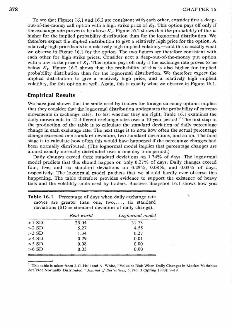
We have just shown that the smile used by traders for foreign currency options impliesthat they consider that the lognormal distribution understates the probability of extrememovements in exchange rates. To test whether they are right, Table 16.1 examines thedaily movements in 12 different exchange rates over a lO-year period? The first step inthe production of the table is to calculate the standard deviation of daily percentagechange in each exchange rate. The next stage is to note how often the actual percentagechange exceeded one standard deviation, two standard deviations, and so on. The finalstage is to calculate how often this would have happened if the percentage changes hadbeen normally distributed. (The lognormal model implies that percentage changes arealmost exactly normally distributed over a one-day time period.)

Daily changes exceed three standard deviations on 1.34% of days. The lognormalmodel predicts that this should happen on only 0.27% of days. Daily changes exceedfour, five, and six standard deviations on 0.29%, 0.08%, and 0.03% of days,respectively. The lognormal model predicts that we should hardly ever observe thishappening. The table therefore provides evidence to support the existence of heavytails and the volatility smile used by traders. Business Snapshot 16.1 shows how you

Table 16.1 Percentage of days when daily exchange ratemoves are greater than one, two, . . . , six standarddeviations (SD = standard deviation of daily change).

Real world Lognormal model

> l S D 25.04 31.73>2SD 5.27 4.55>3SD 1.34 0.27>4SD 0.29 om>5SD 0.08 0.00

>6SD 0.03 0.00

2 This table is taken from J. C. Hull and A, White, "Value at Risk When Daily Changes in Market VariablesAre-Not Normally Distributed," Journal of Derivatives, 5, No, 3 (Spring 1998): 9-19,




could have made money if you had done the analysis in Table 16.1 ahead of the restof the market.

Reasons for the Smile in Foreign Currency Options

Why are exchange rates not lognormally distributed? Two of the conditions for an assetprice to have a lognormal distribution are:

1. The volatility of the asset is constant.2. The price of the asset changes smootWy with no jumps.

In practice, neither of these conditions is satisfied for an exchange rate. The volatility ofan exchange rate is far from constant, and exchange rates frequently exhibit jumps? I t

turns out that the effect of both a nonconstant volatility and jumps is that extremeoutcomes become more likely. The impact of jumps and nonconstant volatility dependson the option maturity. The percentage impact of a nonconstant volatility on pricesbecomes more pronounced as the maturity of the option is increased, but the volatility

smile created by the nonconstant volatility usually becomes less pronounced. Thepercentage impact of jumps on bo th prices and the volatility smile becomes lesspronounced as the maturity of the option is increased. When we look at sufficientlylong-dated options, jumps tend to get "averaged out" so that the stock price distribution when there are jumps is almost indistinguishable from the one obtained when thestock price changes smootWy . .

16.3 EQUITY OPTIONS

The volatility smile for equity options has been studied by Rubinstein (1985, 1994) andJackwerth and Rubinstein (1996). Prior to 1987 there was no marked volatility smile.

3 Often the jumps are in response to the actions of central banks.



380 CHAPTER 16

Figure 16.3 Volatility smile for equities.

Impliedvolatility

Strike price

Since 1987 the volatility smile used by traders to. price equity options (both on individualstocks and on stock indices) has the general form shown in Figure 16.3. This is sometimesreferred to as a volatility skew. The volatility decreases as the strike price increases. Thevolatility used to price a low-strike-price option (i.e., a deep-out-of-the-money put or adeep-in-the-money call) is significantly higher than that used to price a high-strike-priceoption (i.e., a deep-in-the-money put or a deep-out-of-the-money call).

The volatility smile for equity options corresponds to the implied probability distribution given by the solid line in Figure 16.4. A lognormal distribution with the same

Figure 16.4 Implied distribution and lognormal distribution for equity options.

\\\\

\ _ Lognormal\ \

\

""-"

' -




mean and standard deviation as the implied distribution is shown by the dotted line. I t

can be seen that the implied distribution has a heavier left tail and a less heavy right tailthan the lognormal distribution.

To see that Figures 16.3 and 16.4 are consistent with each other,we proceed as forFigures 16.1 and 16.2 and consider options that are deep out of the money. FromFigure 16.4 a deep-out-of-the-money call with a strike price of K2 has a lower pricewhen the implied distribution is used than when the lognormal distribution is used. Thisis because the option pays off only if the stock price proves to be above K 2 , and theprobability of this is lower for the implied probability distribution than for the lognormaldistribution. Therefore, we expect the implied distribution to give a relatively low pricefor the option. A relatively low price leads to a relatively low implied volatility-and thisis exactly what we observe in Figure 16.4 for the option. Consider next a deep-out-of-the

money put option with a strike price of K\. This option pays off only if the stock priceproves to be below K\. Figure 16.3 shows that the probability of this is higher for impliedprobability distribution than for the lognormal distribution. We therefore expect theimplied distribution to give a relatively high price, and a relatively high implied volatility,for this option. Again, this is exactly what we observe in Figure 16.3.

The Reason for the Smile in Equity Options

One possible explanation for the smile in equity options concerns leverage. As acompany's equity declines in value, the company's leverage increases. This means thatthe equity becomes more risky and its volatility increases. As a company's equityincreases in value, leverage decreases. The equity then becomes less risky and itsvolatility decreases. This argument shows that we can expect the volatility of equityto be a decreasing function of price and is consistent with Figures 16.3 and 16.4.Another explanation is crashophobia (see Business Snapshot 16.2).

16.4 THE VOLATILITY TERM STRUCTURE AND VOLATILITY SURFACES

In addition to a volatility smile, traders use a volatility term structure when pricingoptions. This means that the volatility used to price an at-the-money option depends onthe maturity of the option. Volatility tends to be an increasing function of maturitywhen short-dated volatilities are historically low. This is because there is then anexpectation that volatilities will increase. Similarly, volatility tends to be an decreasing



_1In(K). jT Fa

382 CHAPTER 16

Table 16.2 Volatility surface.

Strike

0.90 0.95 1.00 1.05 1.10

1 month 14.2 13.0 12.0 13.1 14.5

3 month 14.0 13.0 12.0 13.1 14.26 month 14.1 13.3 12.5 13.4 14.31 year 14.7 14.0 13.5 14.0 14.82 year 15.0 14.4 14.0 14.5 15.15 year 14.8 14.6 14.4 14.7 15.0

function of maturity when short-dated volatilities are historically high. This is becausethere is then an expectation that volatilities will decrease.- Volatility surfaces combine volatility smiles with the volatility term structure totabulate the volatilities appropriate for pricing an option with any strike price andany maturity. An example of a volatility surface that might be used for foreign currencyoptions is given in Table 16.2.

One dimension of Table 16.2 is strike price; the other is time to maturity. The mainbody of the table shows implied volatilities calculated from the Black-Sc1:).oles model.At any given time, some of the entries in the table are likely to correspond to optionsfor which reliable market data are available_. The implied volatilities for these optionsare calculated directly from their market prices and entered into the table. The rest of

the table is determined using linear interpolation.

When a new option has to be valued, financial engineers look up the appropriatevolatility in the table. For example, when valuing a 9-month option with a strike priceof 1.05, a financial engineer would interpolate between 13.4 and 14.0 in Table 16.2 toobtain a volatility of 13.7%. This is the volatility that would be used in the BlackScholes formula or a binomial tree.

The shape of the volatility smile depends on the option maturity. As illustrated inTable 16.2, the smile tends to become less pronounced as the option maturity increases.Define T as the time to maturity and Fa as the forward price of the asset. Some financialengineers choose to define the volatility smile as the relationship. between impliedvolatility and

rather than as the relationship between the implied volatility and K. The smile is thenusually much less dependent on the time to maturity.4

The Role of the Model

How important is the pricing model if traders are prepared to use a different volatilityfor every option? I t can be argued that the Black-Scholes model is no more than a

sophisticated interpolation tool used by traders for ensuring that an option is priced

4 Fo r a discussion of this approach, see S. Natenberg Option Pricing and Volatility: Advanced TradingStrategies and Techniques, 2nd edn. McGraw-Hill, 1994; R. Tompkins Options Analysis: A State o j the ArtGuide fo Options Pricing, Burr Ridge, IL: Irwin, 1994.




consistently with the market prices of other actively: traded options. I f traders stoppedusing Black-Scholes and switched to another plausible model, then the volatilitysurface and the shape of the smile would change, but arguably the dollar prices quotedin the market would not change appreciably.

16.5 GREEK LETTERS

The volatility smile complicates the calculation of Greek letters. Derman describes anumber of volatility regimes or rules of thumb that are sometimes assumed by traders. 5

The simplest of these is known as the sticky strike rule. This assumes that the impliedvolatility of an option remains constant from one day to the next. I t means that Greekletters calculated using the Black-Scholes assumptions are correct provided that thevolatility used for an option is its current implied volatility.

A more complicated rule is known as the sticky delta rule. This assumes that the

relationshipwe

observe between an option price andSf K

today will apply tomorrow. Asthe price of the underlying asset changes, the implied volatility of the option is assumedto change to reflect the option's "moneyness" (i.e., the extent to which it is in or out of

the money). I f we use the sticky delta rule, the formulas for Greek letters given in theChapter 15 are no longer correct. Fo r example, delta of a call option is given by

aCBS aCBS aaimp- + - - - -

as aaimp as

where CBS is the Black-Scholes price of the option expressed as a function of the asset

price S and the implied volatility aimp. Consider the impact of this formula on the delta ofan equity call option. From Figure 16.3, volatility is a decreasing function of the strikeprice K. Alternatively it can be regarded as .an increasing function of Sf K. Under thesticky delta model, therefore, the volatility increases as the asset price increases, so that

aaimp 0- - >

as

As a result, delta is higher than that given by the Black-Scholes assumptions.I t turns out that the sticky strike and sticky delta rules do not correspond to internally

consistent models (except when the volatility smile is flat for all maturities). A modelthat can be made exactly consistent with the smiles is known as the implied volatilityjunction model or the implied tree model. We will explain this model in Chapter 24.

In practice, banks try to ensure that their exposure to the most commonly observedchanges in the volatility surface is reasonably small. One technique for identifying thesechanges is principal components analysis, which we discuss in Chapter 18.

16.6 WHEN A SINGLE LARGE JUMP IS ANTICIPATED

Let us now consider an example of how an unusual volatility smile might arise inequity markets. Suppose that a stock price is currently $50 and an important news

5 See E. Derman, "Regimes of Volatility," Risk, April 1999, 54-59



384 CHAPTER 16

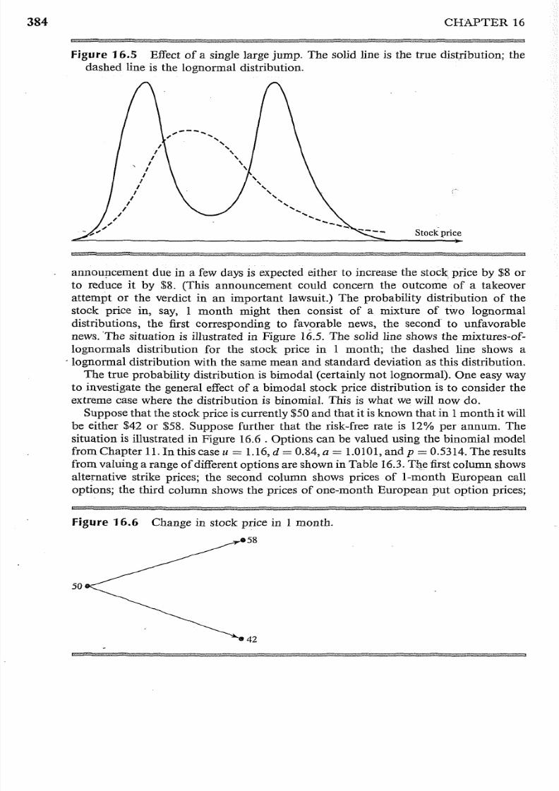
Figure 16.5 Effect of a single large jump. The solid line is the true distribution; thedashed line is the lognormal distribution.

; 1 " - - - ......... ,,

,,

,,

,

Stock price

annou!1cement due in a few days is expected either to increase the stock price by $8 orto reduce i t by $8. (This announcement could concern the outcome of a takeoverattempt or the verdict in an important lawsuit.) The probability distribution of thestock price in, say, 1 month might then consist of a mixture of two lognormaldistributions, the first corresponding to favorable news, the second to unfavorablenews. 'The situation is illustrated in Figure 16.5. The solid line shows the mixtures-oflognormals distribution for the stock price in 1 month; the dashed line shows a

. lognormal distribution with the same mean and standard deviation as this distribution.The true probability distribution is bimodal (certainly not lognormal). One easy way

to investigate the general effect of a bimodal stock price distribution is to consider theextreme case where the distribution is binomial. This is what we will now do.

Suppose that the stock price is currently $50 and that it is known that in 1 month it willbe either $42 or $58. Suppose further that the risk-free rate is 12% per annum. Thesituation is illustrated in Figure 16.6 . Options can be valued using the binomial modelfrom Chapter 11. In this case u = 1.16, d = 0.84, a = 1.0101, and p = 0.5314. The resultsfrom valuing a range of different options are shown in Table 16.3.T4e first column shows

alternative strike prices; the second column shows prices of I-month European calloptions; the third column shows the prices of one-month European put option prices;

Figure 16.6 Change in stock price in 1 month.

58

50

42



Volatility Stniles 385

Table 16.3 Implied volatilities in situation where true distributionis binomial.

Strike price($)

Call price($)

Put price($)

Implied volatility(% )

42

44

46

485052545658

8.427.376.31

5.264.21

3.162.101.050.00

0.000.931.862.78

3.71

4.645.576.507.42

0.058.866.669.569.266.1

60.049.0

0.0

the fourth column shows implied volatilities. (As shown in Section 16.1, the impliedvolatility of a European put option is the same as that of a European call option whenthey have the same strike price and maturity.) Figure 16.7 shows the volatility smile. I t isactually a "frown" (the opposite of that observed for currencies) with volatilitiesdeclining as we move out of or into the money. The volatility implied from an optionwith a strike price of 50 will overprice an option with a strike price of 44 or 56.

SUMMARY

The Black-Scholes model and its extensions assume that the probability distribution ofthe underlying asset at any given future time is lognormal. This assumption is not the

Figure 16.7 Volatility smile for situation in Table 16.3.

90Implied

80volatility (%)

70

60

50

40

30

20

10

Strike price0

44 46 48 50 52 54 56



386 CHAPTER 16

one made by traders. They assume the probability distribution of an equity price has aheavier left tail and a less heavy right tail than the lognormal distribution. They alsoassume that the probability distribution of an exchange rate has a heavier right tail anda heavier left tail than the lognormal distribution.

Traders use volatility smiles to allow for nonlognormality. The volatility smile defines

the relationship between the implied volatilityof

an option and its strike price.Fo r

equity options, the volatility smile tends to be downward sloping. This means that outof-the-money puts and in-the-money calls tend to have high implied volatilities whereasout-of-the-money calls and in-the-money puts tend to have low implied volatilities. Fo r

foreign currency options, the volatility smile is U-shaped. Both out-of-the-money andin-the-money options have higher implied volatilities than at-the-money options.

Often traders also use a volatility term struGture. The implied volatility of an optionthen depends on its life. When volatility smiles and volatility term structures arecombined, they produce a volatility surface. This defines implied volatility as a functionQ.f both the strike price and the time to maturity.

FURTHER READING

Bakshi, G., C. Cao, and Z. Chen. "Empirical Performance of Alternative Option PricingModels," Journal o f Finance, 52, No.5 (December 1997): 2004-49.

Bates, D. S. "Post-'87 Crash Fears in the S&P Futures Market," Journal of Econometrics, 94(Jap.uaryjFebruary 2000): 181-238.

Derman, E. "Regimes of Volatility," Risk, April 1999: 55-59.

Ederington, L. H., and W. Guan. "Why Are Those Options Smiling," Journal o f Derivatives, 10,2 (2002): 9-34.

Jackwerth, J. C., and M. Rubinstein. "Recovering Probability Distributions from OptionPrices," Journal of Finance, 51 (December 1996): 1611-31.

Lauterbach, B., and P. Schultz. "Pricing Warrants: An Empirical Study of the Black-ScholesModel and Its Alternatives," Journal o f Finance, 4, No.4 (September 1990): 1181-1210.

Melick, W. R., and C. P. Thomas. "Recovering an Asset's Implied Probability Density Functionfrom Option Prices: An Application to Crude Oil during the Gulf Crisis," Journal o f Financialand Quantitative Analysis, 32, 1 (March 1997): 91-115.

Rubinstein, M. "Nonparametric Tests of Alternative Option Pricing Models Using AlI Reported

Trades and Quotes on the 30 Most Active CBOE Option Classes from August 23, 1976,through August 31, 1978," Journal o f Finance, 40 (June 1985): 455-80.

Rubinstein, M. "Implied Binomial Trees," Journal of Finance, 49, 3 (July 1994): 771-818.Xu, x., and S. J. Taylor. "The Term Structure of Volatility Implied by Foreign Exchange

Options," Journal o f Financial and Quantitative Analysis, 29 (1994): 57-74.

Questions and Problems (Answers in Solutions Manual)

16.1. What volatility smile is likely to be observed when:(a) Both tails of the stock price distribution are less heavy than those of the lognormal

distribution?(b) The right tail is heavier, and the left tail is less heavy, than that of a lognormal

distribution?



Volatility Smiles

16.2. What volatility smile is observed for equities?

387

16.3.

16.4.

16.5.

16.6.

16.7.

16.8.

16.9.

16.10.

16.11.

16.12.

16.13.

16.14.

16.15.

What volatility smile is likely to be caused by jumps in the underlying asset price? Is thepattern likely to be more pronounced for a 2-year option than fdr a 3-month option?A European call and pu t option have the same strike price and time to maturity. The callhas an implied volatility of 30% and the put has an implied volatility of 25%. What

trades would you do?Explain carefully why a distribution with a heavier left tail and less heavy right tail thanthe lognormal distribution gives rise to a downward sloping volatility smile.The market price of a European call is $3.00 and its price given by Black-Scholes modelwith a volatility of 30% is $3.50. The price given by this Black-Scholes model for aEuropean pu t option with the same strike price and time to maturity is $1.00. Whatshould the market price of the put option be? Explain the reasons for your answer.Explain what is meant by "crashophobia".

A stock price is currently $20. Tomorrow, news is expected to be announced that willeither increase the price by $5 or decrease the price by $5. What are the problems inusing Black-Scholes to value I-month options on the stock?What volatility smile is likely to be observed for 6-month options when the volatility isuncertain and positively correlated to the stock price?

What problems do you think would be encountered in testing a stock option pricingmodel empirically?Suppose that a central bank's policy is to allow an exchange rate to fluctuate between0.97 and 1.03. What pattern of implied volatilities for options on the exchange ratewould you expect to see?

Option traders sometimes refer to deep-out-of-the-money options as being options onvolatility. Why do you think they do this?A European call option on a certain stock has a strike price of $30, a time to maturity of1 year, and an implied,volatility of 30%. A European put option on the same stock has astrike price of $30, a time to maturity of 1 year, and an implied volatility of 33%. Whatis the arbitrage opportunity open to a trader? Does the arbitrage work only when thelognormal assumption underlying Black-Scholes holds? Explain carefully the reasons

for your answer.Suppose that the result of a major lawsuit affecting Microsoft is due to be announcedtomorrow. Microsoft's stock price is currently $60. If the ruling is favorable toMicrosoft, the stock price is expected to jump to $75. If it is unfavorable, the stock isexpected to jump to $50. What is the risk-neutral probability of a favorable ruling?Assume that the volatility of Microsoft's stock will be 25% for 6 months after the rulingif the ruling is favorable and 40% if it is unfavorable. Use DerivaGem to calculate therelationship between implied volatility and. strike price for 6-month European options onMicrosoft today. Microsoft does not pay dividends. Assume that the 6-month risk-freerate is 6%. Consider call options with strike prices of 30, 40, 50, 60, 70, and 80.

An exchange rate is currently 0.8000. The volatility of the exchange rate is quoted as12% and interest rates in the two countries are the same. Using the lognormalassumption, estimate the probability that the exchange rate in 3 months will be (a) lessthan 0.7000, (b) between 0.7000 and 0.7500, (c) between 0.7500 and 0.8000, (d) between



388 CHAPTER 16

0.8000 and 0.8500, (e) between 0.8500 and 0.9000, and (f ) greater than 0.9000. Based onthe volatility smile usually observed in the market for exchange rates; which of theseestimates would you expect to be too low and which would you expect to be too high?

16.16. A stock price is $40. A 6-month European call option on the stock with a strike price of

$30 has an implied volatility of 35%. A 6-month European call option on the stock witha strike price of $50 has an implied volatility of 28%. The 6-month risk-free rate is 5%and no dividends are expected. Explain why the two implied volatilities are different. UseDerivaGem to calculate the prices of the two options. Use put-eall parity to calculatethe prices of 6-month European put options with strike prices of $30 and $50. UseDerivaGem to calculate the implied volatilities of these two put options.

16.17. "The Black-Scholes model is used by traders as an interpolation tool." Discuss this view.

Assignment Questions16.18. A company's stock is selling for $4. The company has no outstanding debt. Analysts

consider the liquidation value of the company to be at least $300,000 and there are100,000 shares outstanding. What volatility smile would you expect to see?

16.19. A company is currently awaiting the outcome of a major lawsuit. This is expected to beknown within 1 month. The stock price is currently $20. If the outcome is positive, thestock price is expected to be $24 at the end of 1 month. If the outcome is negative, it isexpected to be $18 at this time. The I-month risk-free interest rate is 8% per annum.(a) What is the risk-neutral probability of a positive outcome?(b) What are the values of I-month call options with strike prices of $19, $20, $21,$22,

and $23?(c) Use DerivaGem to calculate a volatility smile for I-month call options.(d) Verify that the same volatility smile is obtained for I-month put options.

16.20. A futures price is currently $40. The risk-free interest rate is S%. Some news is expectedtomorrow that will cause the volatility over the next 3 months to be either 10% or 30%.There is a 60% chance of the first outcome and a 40% chance of the second outcome.Use DerivaGem to calculate a volatility smile for 3-month options.

16.21. Data for a number of foreign currencies are provided on the author'sw e b ~ t t e :

h t t p : / / w w w . r o t m a n . u t o r o n t o . c a / ~ h u l l

Choose a currency and use the data to produce a table similar to Table 16.1.16.22. Data for a number of stock indices are provided on the author's website:

h t t p : / / w w w . r o t m a n . u t o r o n t o . c a / ~ h u l l

Choose an index and test whether a three-standard-deviation down movement happensmore often than a three-standard-deviation up movement.

16.23. Consider a European call and a European put with the same strike price and time to

maturity. Show that they change in value by the same amount when the volatilityincreases from a level (J l to a new level (J2 within a short period of time. (Hint: Useput-eall parity.)



Volatility Smiles

APPENDIX

DETERMINING IMPLIED RISK-NEUTRAL DISTRIBUTIONSFROM VOLATILITY SMILES r

389

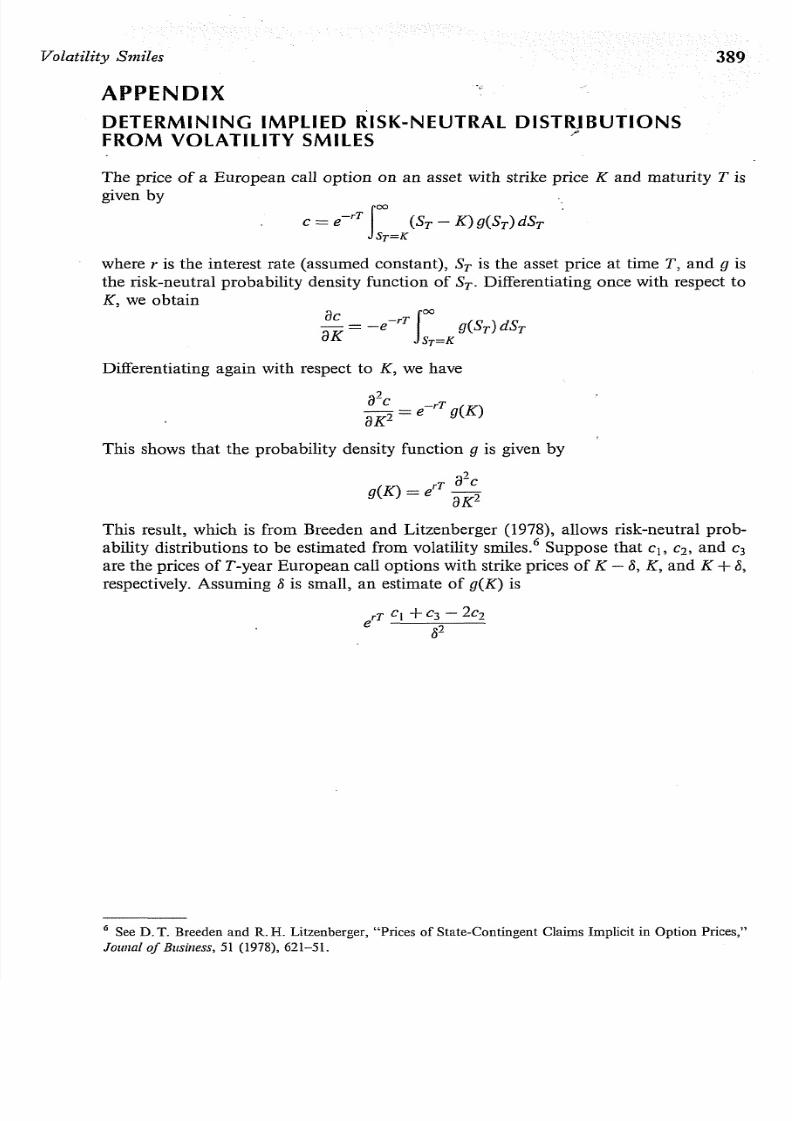
The price of a European call option on an asset with strike price K and maturity T isgiven by

where r is the interest rate (assumed constant), ST is the asset price at time T, and g isthe risk-neutral probability density function of ST' Differentiating once with respect toK, we obtain

ac -rT Joo ( )aK

= - e g ST dSTST=K

Differentiating again with respect to K, we have

a2c _ - rT (K )

aK 2 - e g

This shows that the probability density function g is given by

(K) rT a2c

g = e aK 2

This result, which is from Breeden and Litzenberger (1978), allows risk-neutral probability distributions to be estimated from volatility smiles. 6 Suppose that C b C2, and C3

are the prices of T-year European call options with strike prices of K - 8, K, and K + 8,respectively. Assuming 8 is small, an estimate of g(K) is

6 See D. T. Breeden and R. H. Litzenberger, "Prices of State-Contingent Claims Implicit in Option Prices,"

16 Volatility Smiles

Documents

Transcript of 16 Volatility Smiles