16-QAM Hierarchical Modulation Optimization in Relay ... · 16-QAM Hierarchical Modulation...
175
16-QAM Hierarchical Modulation Optimization in Relay Cooperative Networks by Sara Sallam A Thesis In the Department of Electrical and Computer Engineering Presented in Partial Fulfillment of the Requirements for the Degree of Master of Applied Sciences at Concordia University Montreal, Quebec, Canada March 2013 © Sara Sallam, 2013
Transcript of 16-QAM Hierarchical Modulation Optimization in Relay ... · 16-QAM Hierarchical Modulation...
16-QAM Hierarchical Modulation Optimization in
Relay Cooperative Networks
by
Sara Sallam
A Thesis
In the Department
of
Electrical and Computer Engineering
Presented in Partial Fulfillment of the Requirements
for the Degree of Master of Applied Sciences at
Concordia University
Montreal, Quebec, Canada
March 2013
© Sara Sallam, 2013
CONCORDIA UNIVERSITY
SCHOOL OF GRADUATE STUDIES
This is to certify that the thesis prepared
By: Sara Sallam
Entitled: “16-QAM Hierarchical Modulation Optimization in Relay Cooperative
Networks”
and submitted in partial fulfillment of the requirements for the degree of
Master of Applied Science
Complies with the regulations of this University and meets the accepted standards with respect to
originality and quality.
Signed by the final examining committee:
________________________________________________ Chair
Dr. R. Raut
________________________________________________ Examiner, External
Dr. F. Haghighat, BCEE To the Program
________________________________________________ Examiner
Dr. W. Hamouda
________________________________________________ Supervisor
Dr. M. R. Soleymani
Approved by: ___________________________________________
Dr. W. E. Lynch, Chair
Department of Electrical and Computer Engineering
____________20_____ ___________________________________
Dr. Robin A. L. Drew
Dean, Faculty of Engineering and
Computer Science
iii
Abstract
16-QAM Hierarchical Modulation Optimization in Relay Cooperative Networks
Sara Sallam
Recently, the concept of cooperative networks has attracted special attention in the
field of wireless communications. This is due to their ability in achieving diversity with
no extra hardware cost. The main drawback that characterizes cooperative networks is
that they require extra transmission time slots compared to the traditional non-
cooperative networks. Several strategies have been proposed in order to mitigate this
disadvantage. One of the most recently adopted techniques is the use of hierarchical
modulation. Hierarchical modulation was originally used in Digital Video Broadcast
(DVB) applications. Lately, it has been applied in cooperative networks for its ability to
transmit relative high data rate with acceptable performance.
In this thesis, the application of a 4/16 QAM hierarchical modulation in
cooperative networks is examined. This study focuses on a downlink cellular network
scenario, composed of a Base Station, a Relay and two destinations. The Base Station
intends to transmit two different streams of data to these two destinations by
concatenating the two streams and broadcasting the resulting sequence using a non-
uniform 4/16 QAM hierarchical modulation. Unlike previous work, the main
contribution in this thesis is the optimization of the 16QAM constellation’s parameters
according to each user’s channel condition. In other words, this method gives each
user’s data the priority it needs in order to be detected as correctly as possible at the
destination. Explicit closed form expressions of Hierarchical modulation Bit Error Rate
iv
in relay cooperative networks are derived. These BER expressions are used in order to
select the constellation’s parameters that will achieve total minimum BER in coded and
un-coded schemes. Results prove that the proposed method achieve noticeable
improvement in both users performance compared to the use of uniform 16QAM
constellation.

v
To my mother

vi
Acknowledgments
This thesis and the effort exerted in it would not have been completed without the
help, guidance, support and motivation of several individuals who have generously
provided their appreciated assistance in presenting this work the way it is today.
First and foremost, I would like to express my sincere and ultimate gratitude to
my advisor Prof. Dr. M. Reza Soleymani for his continuous support throughout my
research work, for his close follow-up, time, effort, criticism, knowledge sharing and
expertise and continuous motivation. Without his support and guidance it would have
been difficult to finish this thesis and to achieve the results achieved.
I owe my deepest gratitude to Dr. Mojtaba Kahrizi for his kind support,
consideration and availability for advice and assistance. I would like to specially thank
Ms. Diane Moffat for her wonderful support, her continuous assistance and her lovely
smile. She has turned really bad days into wonderful ones. My greatest appreciations
and thanks go to my committee members for their effort and time.
I’m also utterly thankful to my colleagues in the wireless and satellite
communications lab. They have been always ready to willingly offer their knowledge
and support. Special thanks go to my colleague Hesam Khoshneviss for his sense of
humor mixed with his deep scientific knowledge that gave me brighter days.
Last but not the least, my deepest gratitude entitled to my wonderful family; my
most amazing mother Iman and my lovely sisters Yomna, Farah and Hana for their belief
in me, their encouragement, support, patience and motivating smiles in times of stress. I
love you all so much.

vii
I would also like to thank all my friends here in Canada and in Egypt who have
been continuously supporting and encouraging me at all time. Thank you all.
Finally, my infinite gratitude to my dear God, for answering my prayers and
giving me the strength and the patience to continue this work despite the hardest times
when I just wanted to give it all up. Thank you so much dear God.
viii
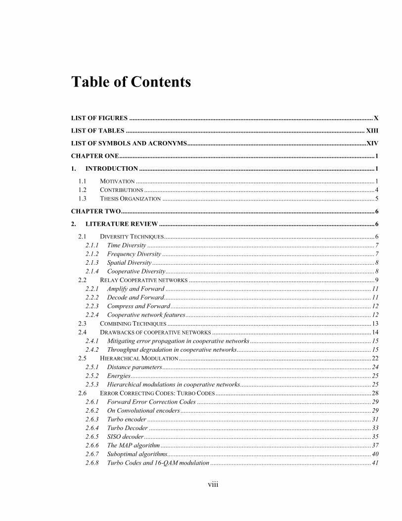
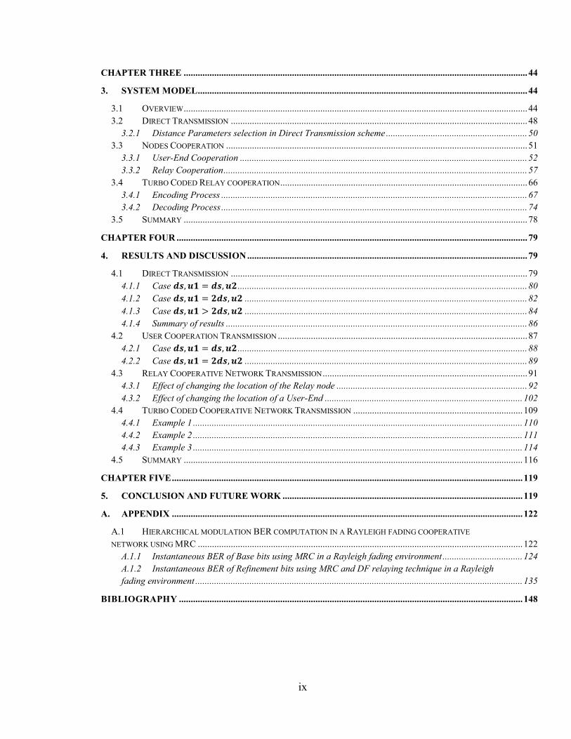
Table of Contents
LIST OF FIGURES ................................................................................................................................................... X
LIST OF TABLES ................................................................................................................................................ XIII
LIST OF SYMBOLS AND ACRONYMS ............................................................................................................ XIV
CHAPTER ONE .......................................................................................................................................................... 1
1. INTRODUCTION .............................................................................................................................................. 1
1.1 MOTIVATION ................................................................................................................................................ 1
1.2 CONTRIBUTIONS ........................................................................................................................................... 4
1.3 THESIS ORGANIZATION ................................................................................................................................ 5
CHAPTER TWO ......................................................................................................................................................... 6
2. LITERATURE REVIEW .................................................................................................................................. 6
2.1 DIVERSITY TECHNIQUES ............................................................................................................................... 6
2.1.1 Time Diversity ......................................................................................................................................... 7
2.1.2 Frequency Diversity ................................................................................................................................ 7
2.1.3 Spatial Diversity ...................................................................................................................................... 8
2.1.4 Cooperative Diversity .............................................................................................................................. 8
2.2 RELAY COOPERATIVE NETWORKS ................................................................................................................ 9
2.2.1 Amplify and Forward ............................................................................................................................ 11
2.2.2 Decode and Forward ............................................................................................................................. 11
2.2.3 Compress and Forward ......................................................................................................................... 12
2.2.4 Cooperative network features ................................................................................................................ 12
2.3 COMBINING TECHNIQUES ........................................................................................................................... 13
2.4 DRAWBACKS OF COOPERATIVE NETWORKS ................................................................................................ 14
2.4.1 Mitigating error propagation in cooperative networks ......................................................................... 15
2.4.2 Throughput degradation in cooperative networks ................................................................................. 15
2.5 HIERARCHICAL MODULATION .................................................................................................................... 22
2.5.1 Distance parameters .............................................................................................................................. 24
2.5.2 Energies ................................................................................................................................................. 25
2.5.3 Hierarchical modulations in cooperative networks ............................................................................... 25
2.6 ERROR CORRECTING CODES: TURBO CODES .............................................................................................. 28
2.6.1 Forward Error Correction Codes ......................................................................................................... 29
2.6.2 On Convolutional encoders ................................................................................................................... 29
2.6.3 Turbo encoder ....................................................................................................................................... 31
2.6.4 Turbo Decoder ...................................................................................................................................... 33
2.6.5 SISO decoder ......................................................................................................................................... 35
2.6.6 The MAP algorithm ............................................................................................................................... 37
2.6.7 Suboptimal algorithms ........................................................................................................................... 40
2.6.8 Turbo Codes and 16-QAM modulation ................................................................................................. 41
ix
CHAPTER THREE .................................................................................................................................................. 44
3. SYSTEM MODEL ............................................................................................................................................ 44
3.1 OVERVIEW .................................................................................................................................................. 44
3.2 DIRECT TRANSMISSION .............................................................................................................................. 48
3.2.1 Distance Parameters selection in Direct Transmission scheme ............................................................ 50
3.3 NODES COOPERATION ................................................................................................................................ 51
3.3.1 User-End Cooperation .......................................................................................................................... 52
3.3.2 Relay Cooperation ................................................................................................................................. 57
3.4 TURBO CODED RELAY COOPERATION ......................................................................................................... 66
3.4.1 Encoding Process .................................................................................................................................. 67
3.4.2 Decoding Process .................................................................................................................................. 74
3.5 SUMMARY .................................................................................................................................................. 78
CHAPTER FOUR ..................................................................................................................................................... 79
4. RESULTS AND DISCUSSION ....................................................................................................................... 79
4.1 DIRECT TRANSMISSION .............................................................................................................................. 79
4.1.1 Case ........................................................................................................................... 80
4.1.2 Case ........................................................................................................................ 82
4.1.3 Case ........................................................................................................................ 84
4.1.4 Summary of results ................................................................................................................................ 86
4.2 USER COOPERATION TRANSMISSION .......................................................................................................... 87
4.2.1 Case ........................................................................................................................... 88
4.2.2 Case ........................................................................................................................ 89
4.3 RELAY COOPERATIVE NETWORK TRANSMISSION ....................................................................................... 91
4.3.1 Effect of changing the location of the Relay node ................................................................................. 92
4.3.2 Effect of changing the location of a User-End .................................................................................... 102
4.4 TURBO CODED COOPERATIVE NETWORK TRANSMISSION ........................................................................ 109
4.4.1 Example 1 ............................................................................................................................................ 110
4.4.2 Example 2 ............................................................................................................................................ 111
4.4.3 Example 3 ............................................................................................................................................ 114
4.5 SUMMARY ................................................................................................................................................ 116
CHAPTER FIVE ..................................................................................................................................................... 119
5. CONCLUSION AND FUTURE WORK ...................................................................................................... 119
A. APPENDIX ..................................................................................................................................................... 122
A.1 HIERARCHICAL MODULATION BER COMPUTATION IN A RAYLEIGH FADING COOPERATIVE
NETWORK USING MRC .......................................................................................................................................... 122
A.1.1 Instantaneous BER of Base bits using MRC in a Rayleigh fading environment .................................. 124
A.1.2 Instantaneous BER of Refinement bits using MRC and DF relaying technique in a Rayleigh
fading environment ........................................................................................................................................... 135
BIBLIOGRAPHY .................................................................................................................................................. 148
x
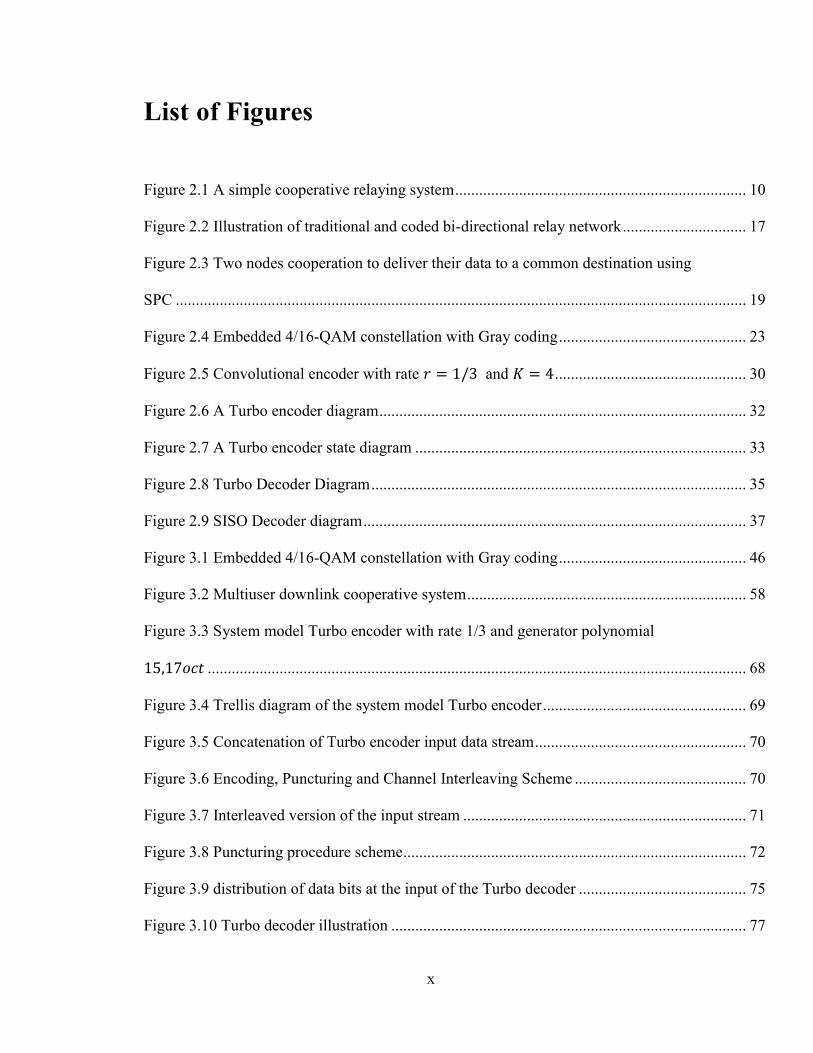
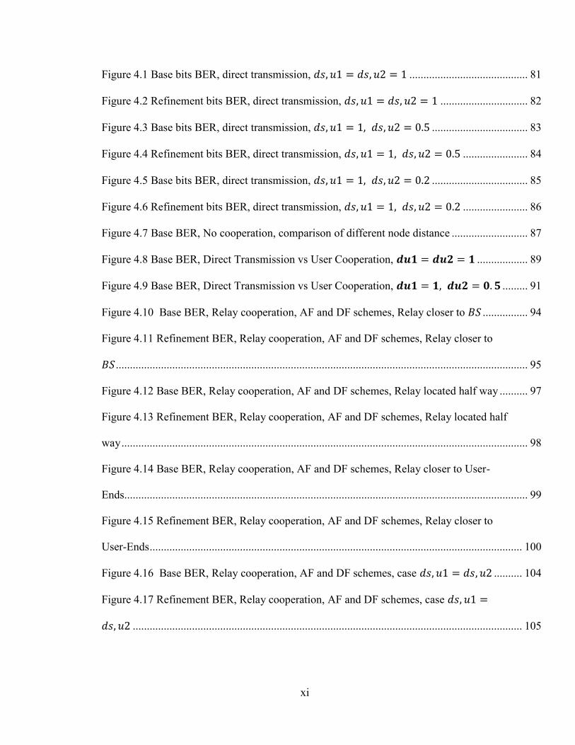
List of Figures
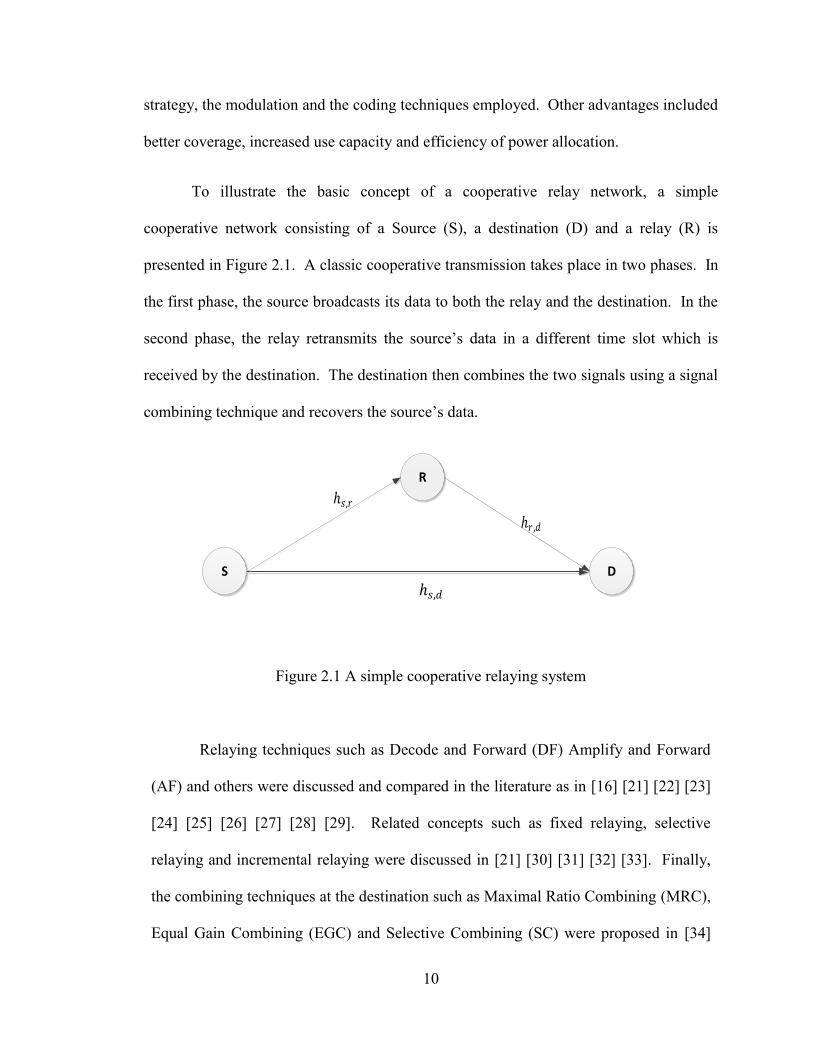
Figure 2.1 A simple cooperative relaying system ......................................................................... 10
Figure 2.2 Illustration of traditional and coded bi-directional relay network ............................... 17
Figure 2.3 Two nodes cooperation to deliver their data to a common destination using
SPC ............................................................................................................................................... 19
Figure 2.4 Embedded 4/16-QAM constellation with Gray coding ............................................... 23
Figure 2.5 Convolutional encoder with rate and ................................................ 30
Figure 2.6 A Turbo encoder diagram ............................................................................................ 32
Figure 2.7 A Turbo encoder state diagram ................................................................................... 33
Figure 2.8 Turbo Decoder Diagram .............................................................................................. 35
Figure 2.9 SISO Decoder diagram ................................................................................................ 37
Figure 3.1 Embedded 4/16-QAM constellation with Gray coding ............................................... 46
Figure 3.2 Multiuser downlink cooperative system ...................................................................... 58
Figure 3.3 System model Turbo encoder with rate 1/3 and generator polynomial
....................................................................................................................................... 68
Figure 3.4 Trellis diagram of the system model Turbo encoder ................................................... 69
Figure 3.5 Concatenation of Turbo encoder input data stream ..................................................... 70
Figure 3.6 Encoding, Puncturing and Channel Interleaving Scheme ........................................... 70
Figure 3.7 Interleaved version of the input stream ....................................................................... 71
Figure 3.8 Puncturing procedure scheme ...................................................................................... 72
Figure 3.9 distribution of data bits at the input of the Turbo decoder .......................................... 75
Figure 3.10 Turbo decoder illustration ......................................................................................... 77
xi
Figure 4.1 Base bits BER, direct transmission, .......................................... 81
Figure 4.2 Refinement bits BER, direct transmission, ............................... 82
Figure 4.3 Base bits BER, direct transmission, .................................. 83
Figure 4.4 Refinement bits BER, direct transmission, ....................... 84
Figure 4.5 Base bits BER, direct transmission, .................................. 85
Figure 4.6 Refinement bits BER, direct transmission, ....................... 86
Figure 4.7 Base BER, No cooperation, comparison of different node distance ........................... 87
Figure 4.8 Base BER, Direct Transmission vs User Cooperation, .................. 89
Figure 4.9 Base BER, Direct Transmission vs User Cooperation, ......... 91
Figure 4.10 Base BER, Relay cooperation, AF and DF schemes, Relay closer to ................ 94
Figure 4.11 Refinement BER, Relay cooperation, AF and DF schemes, Relay closer to
.................................................................................................................................................. 95
Figure 4.12 Base BER, Relay cooperation, AF and DF schemes, Relay located half way .......... 97
Figure 4.13 Refinement BER, Relay cooperation, AF and DF schemes, Relay located half
way ................................................................................................................................................ 98
Figure 4.14 Base BER, Relay cooperation, AF and DF schemes, Relay closer to User-
Ends............................................................................................................................................... 99
Figure 4.15 Refinement BER, Relay cooperation, AF and DF schemes, Relay closer to
User-Ends .................................................................................................................................... 100
Figure 4.16 Base BER, Relay cooperation, AF and DF schemes, case .......... 104
Figure 4.17 Refinement BER, Relay cooperation, AF and DF schemes, case
.......................................................................................................................................... 105
xii
Figure 4.18 Base bits BER, Relay cooperation, AF and DF schemes, case
.......................................................................................................................................... 106
Figure 4.19 Refinement bits BER, Relay cooperation, AF and DF schemes, case
.......................................................................................................................................... 107
Figure 4.20 Base Bits BER, Relay Cooperation, DF relaying at and ............................ 108
Figure 4.21 Base Bits BER, Relay Cooperation, AF relaying at and ............................ 109
Figure 4.22 BER of example1 in un-coded scenario for different values of ......................... 111
Figure 4.23 Average Base BER in Turbo coded scheme, Relay closer to ............................ 115
Figure 4.24 Average Refinement BER in Turbo coded scheme, Relay closer to ................. 116
Figure A.1 A hierarchical 4/16 QAM constellation with Gray mapping ................................... 124
xiii
List of Tables
Table 2-1 XOR Operation ............................................................................................................. 16
Table 4-1 Actual BER of example1 in Turbo coded scenario for different values of .......... 111
Table 4-2 Example2: Theoretical total BER in un-coded scenario for different
constellation’s parameters values ............................................................................................... 113
Table 4-3 Actual BER of example 2 in Turbo coded scenario for different values of .......... 114
xiv
List of Symbols and Acronyms
List of Acronyms
Acronym Explanation
AF Amplify and Forward
ARQ Automatic Repeat Request
AWGN Additive White Gaussian Noise
BCJR Bahl, Cocke, Jelinek and Raviv
BER Bit Error Rate
BPSK Binary Phase Shift Keying
CRC Cyclic Redundancy Check
CSI Channel State Information
DF Decode and Forward
DNF De-noise and Forward
DVB Digital Video Broadcast
EGC Equal Gain Combining
FEC Forward Error Correcting codes
FER Frame Error Rate
HDTV High Definition Television
HPA High Power Amplifiers
LLR Log Likelihood Ratio
MAP Maximum A Posteriori
MIMO Multiple Input Multiple Output
ML Maximum Likelihood
MRC Maximum Ratio Combining
NC Network Coding
PCCC Parallel Concatenated Convolutional Codes
xv
Acronym Explanation
QAM Quadrature Amplitude Modulation
RSC Recursive Systematic Convolutional codes
SC Switch Combining
SER Symbol Error Rate
SISO Soft Input Soft Output
SNR Signal to Noise Ratio
SPC Superposition Coding
UEP Unequal Error Protection
VA Viterbi Algorithm
xvi
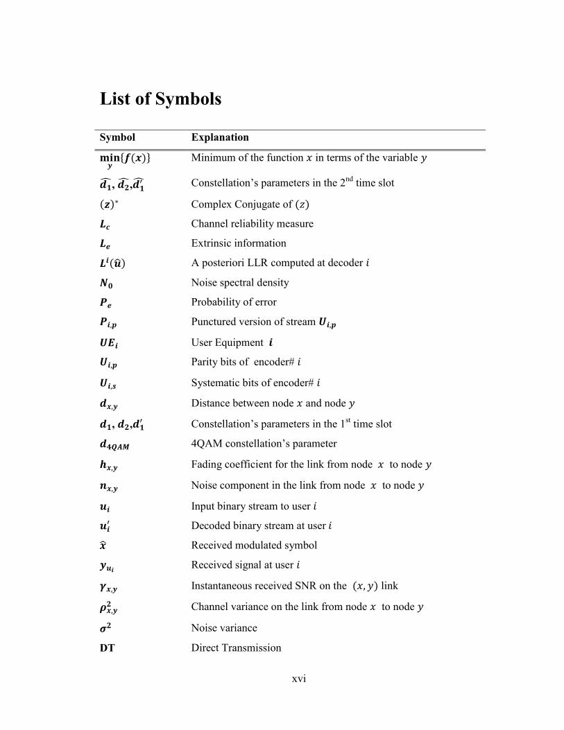
List of Symbols
Symbol Explanation
{ } Minimum of the function in terms of the variable
, , Constellation’s parameters in the 2
nd time slot
Complex Conjugate of
Channel reliability measure
Extrinsic information
A posteriori LLR computed at decoder
Noise spectral density
Probability of error
Punctured version of stream
User Equipment
Parity bits of encoder#
Systematic bits of encoder#
Distance between node and node
, , Constellation’s parameters in the 1
st time slot
4QAM constellation’s parameter
Fading coefficient for the link from node to node
Noise component in the link from node to node
Input binary stream to user
Decoded binary stream at user
Received modulated symbol
Received signal at user
Instantaneous received SNR on the link
Channel variance on the link from node to node
Noise variance
DT Direct Transmission
xvii
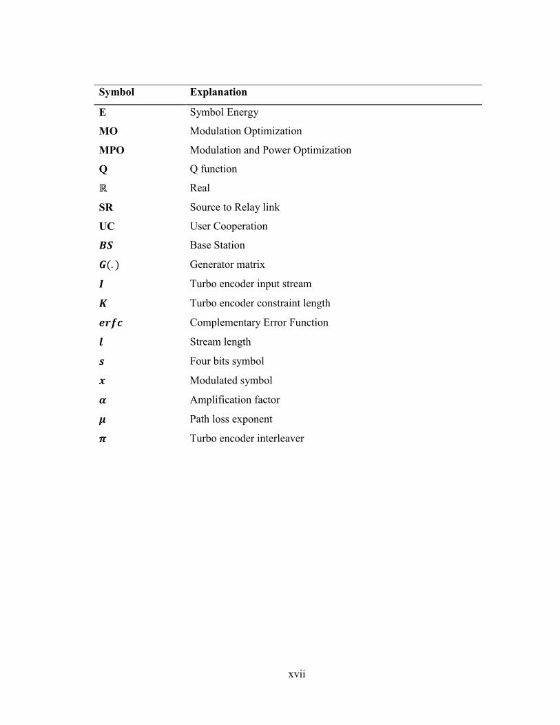
Symbol Explanation
E Symbol Energy
MO Modulation Optimization
MPO Modulation and Power Optimization
Q Q function
Real
SR Source to Relay link
UC User Cooperation
Base Station
Generator matrix
Turbo encoder input stream
Turbo encoder constraint length
Complementary Error Function
Stream length
Four bits symbol
Modulated symbol
Amplification factor
Path loss exponent
Turbo encoder interleaver
1
Chapter One
Introduction 1.
1.1 Motivation
Recently, the high demand on wireless applications has encouraged extensive
research in the wireless communications domain, aiming at analysing and well
understanding the wireless environment in order to be able to provide secure, efficient
and cost effective wireless services. While these studies have contributed considerably
to the development of the present advanced wireless services, more studies are needed
to solve some pertaining problems. One of the major concerns is the signal attenuation
that wireless networks suffer from. Signal attenuations, also known as fading, occur due
to the multipath propagation that the signal experiences in its trajectory from the
transmitter to the destination. Several methods were proposed to mitigate channel
2
fading. In recent years, diversity techniques have received considerable attention due to
their success in mitigating fading effects. Diversity methods are based on transmitting
several copies of the intended signal to the destination. These replicas can be sent on
separate intervals of time, which is known as the time diversity. They can also be
transmitted over different frequency bands, hence referred to as frequency diversity.
Alternatively, they can be sent using multiple transmitting antennas and/or received by
multiple receiving antennas as in Multiple Input Multiple Output (MIMO) systems.
Such a scheme is known as space diversity. Signals can also be sent through different
paths by employing a cooperated multiple nodes transmission scheme that is the
cooperative diversity.
Recently, cooperative diversity has been the most practical method and has proven
to be the most adaptable to the wireless environments demands with no extra hardware
cost. The main disadvantage that characterizes cooperative networks is that they can
require extra transmission time slots when compared to the traditional non-cooperative
networks. In order to improve the throughput of cooperative networks, coding
techniques such as Network Coding (NC) were proposed and extensively studied in the
literature [1] [2] [3] [4]. Network Coding performed well in the case of symmetrical
channel, in other words, where the channels experienced similar fading. On the other
hand, in the case of noticeably dissimilar channels, good channels performance will be
dominated by the channel experiencing the worst fading conditions. More recently
Superposition Coding (SPC) was proposed to work with, and sometimes as an
alternative for, NC. Superposition Coding was first introduced by Cover in [5]. Several
comparisons between SPC and NC were presented in the literature [6] [7] [8]. More
3
developed forms of Superposition Coding such as multi-resolution modulation
techniques were proposed as a modulation technique to work in parallel with
cooperative networks. One of the most employed multi-resolution modulation schemes
is the 4/16 QAM Hierarchical modulation. Hierarchical modulation was proposed for
use in Digital Video Broadcast (DVB) applications in the early 90’s [9]. Recently,
Hierarchical modulation was discussed in the literature to mitigate the fading channel
effect in the cooperative networks scheme. Explicit closed form expressions of
Hierarchical modulation Bit Error Rate (BER) in relay networks were derived in [10].
The BER derivation was expressed in terms of the constellation’s distance parameters.
The authors proposed a criterion to select the distance parameters that will minimize the
refinement bits BER while keeping the error performance of the base bits below a
certain threshold. In [11], a downlink multiuser cooperative communication system was
developed. It consists of a Base Station, a relay and two mobile users. The motivation
behind this paper is to find a method to compensate for the throughput degradation
resulting in the use of relay cooperative systems. The authors suggested employing
Hierarchical Modulation for simultaneous simulation of the data streams of both mobile
users. They mapped one user’s data to the base bits location and the other user’s data to
the refinement bits location. Analysis of the error performance of base bits and
refinement bits was carried in a similar manner as in [10]. They simulated their system
while employing different constellation parameters (the distance between the
constellation points). They compared the base bits and refinement bits performance at
the selected distances. The comparison showed that some distance parameters resulted
in better performance for the base bits at the expense of degradation of the refinement
4
bits performance and vice versa. They suggested the topic of optimal distance
parameters selection as future work.
1.2 Contributions
In this research, a study of the application of a 4/16 QAM hierarchical modulation
in cooperative networks is conducted. This study focuses on a downlink cellular
network scenario, where a Base Station intends to transmit two different streams of data
to two different destinations. These two streams are concatenated together and
modulated using a non-uniform 4/16 QAM hierarchical modulation as in [11]. The
main contribution in this thesis is the optimization of the 16QAM constellation’s
distance parameters according to the channel condition of each user. This
optimization’s goal is to minimize the total Bit Error Rate at the two destinations. In
addition, in the case of multiple transmitting nodes, optimization of the total available
power distribution on these nodes is examined. Several network topologies are
presented in this thesis. First, the concept of optimizing the distance parameters of a
hierarchical modulation is explained in the direct transmission scheme. The effect of
the optimization is clearly illustrated when compared to the non-optimized scenario
(uniform constellation). The performance of the system with the proposed optimization
in the case of non-cooperative and cooperative transmissions is investigated. In the case
of cooperative transmission, the optimization is conducted in the case of Amplify and
Forward (AF) relaying and in the case of Decode and Forward (DF) relaying. Different
nodes location scenarios are examined from the point of view of inter-nodes relative
distances. Comparison between the Bit Error Rate (BER) in the case of optimized
5
constellation and the case of traditional uniform constellation is presented for each case.
Also, the instantaneous probability of error for each stream in the non-cooperative,
cooperative AF and cooperative DF cases are derived. Finally, a preliminary study of
hierarchical modulation optimization in Turbo coded cooperative networks is presented.
In all the above scenarios, optimized constellation always performed better than the
traditional uniform 4/16 QAM constellation.
1.3 Thesis Organization
The remainder of the thesis will be organized as follow. In Chapter 2 we present
the related literature review along with a background on relay networks, diversity
techniques, hierarchical modulation and Turbo codes. In Chapter 3, we present our
system model and our proposed constellation optimization method. In Chapter 4, we
present the different simulations results in the un-coded and coded environment. And
finally in Chapter 5 we conclude our thesis and recommend future work.
6
Chapter Two
Literature Review 2.
In this chapter a detailed literature review and background on the related topics to
the proposed research are presented. The discussed topics in this chapter will include
diversity techniques, cooperative networks, combining techniques, Network Coding,
mutli-resolution modulation and finally Turbo codes.
2.1 Diversity Techniques
Diversity techniques [12], [13] are considered to be the most popular techniques in
combating wireless channel fading. The concept of diversity is based on sending one or
more redundant copies of the transmitted signal in a way that these copies experience
7
different channel fading conditions. In the case where one of the paths experiences deep
fading, there is a chance that other paths will experience better channel conditions and
thus the signal can be recovered reliably at the destination. In other words, assuming
there exists branches through which the message can travel and experience independent
fading conditions. Then the probability of error on any of these branches is denoted by ,
where . The total error probability of the branches is denoted by where
. Therefore the probability of error is seen to be inversely proportional to the
power of the average signal to noise ratio. Hence, the diversity techniques are said to
improve the performance of the given system. Diversity can be accomplished through
several methods. These methods include time diversity, frequency diversity, space
diversity and cooperative diversity.
2.1.1 Time Diversity
In time diversity, the signal is repeatedly transmitted over different time intervals.
The separating time between any two transmissions need to be greater than the coherence
time of the channel. This is to give a chance for variations in the channel conditions to
occur and thus insure that any two replicas experience different fading. However, this
method might suffer from delays, where the delay depends highly on the coherence time
of the channel and on the number of replicas to be sent. In systems where delay is not
tolerable, time diversity technique is not a suitable option.
2.1.2 Frequency Diversity
In frequency diversity replicas of the signal are transmitted over different frequency
carriers. As in the case of time diversity, the separation between any two frequency
8
carriers needs to be greater than the coherence bandwidth of the channel. This is to
assure that each copy of the signal goes through independent fading. However,
frequency diversity requires extra bandwidth which is very scarce in wireless systems and
in some applications it is even impossible to allocate. Also, frequency diversity entails
extra transmitter/receiver for every frequency carrier which adds more to the hardware
cost.
2.1.3 Spatial Diversity
Spatial diversity is accomplished by having multiple antennas at the
transmitter/receiver. It is more advantageous than time and frequency diversity as it does
not require any extra bandwidth and does not suffer from any delays. Multiple Input
Multiple Output (MIMO) is one of the spatial diversity applications and it has proven to
offer relatively a large capacity increase in comparison to single antenna systems.
However, spatial diversity has its own limitations as it requires multiple antennas and
physical separating distance between theses antennas to ensure different fading by each
signal which is not practical in some of the wireless equipment.
2.1.4 Cooperative Diversity
Cooperative diversity is another form of diversity methods. It uses relays;
intermediary nodes, to assist the source in the transmission of the signal. At the
destination, the receiver will have one replica from the source; if possible, and a replica
from each cooperating relay. Cooperative diversity is mainly used to enhance the
coverage when the link between the source and the destination is in a deep fading
condition. Also, the concept of using an intermediary node is advantageous as it divides
9
the separating distance between the source and the destination into multiple hops; which
reduces significantly the signal attenuation. Finally, the separating physical distance
between the source and any intermediary node is large enough so that each replica of the
signal is guaranteed to experience independent fading and thus achieves diversity. In
the following section, cooperative diversity is discussed in more details, illustrating a
simplified cooperative network, presenting the most common relaying protocols and
listing the advantages of cooperative networks in the wireless medium.
2.2 Relay Cooperative networks
In cooperative networks, one or more nodes of the network are employed as relay
nodes in order to assist the transmitter in delivering its data to the receiver with more
reliability. This concept was firstly introduced by van der Meulen in 1971 [14]. He
presented a cooperative transmission scheme where the source sends its data to the
destination through two different paths. Those are the “source to destination” path and
the “source to relay to destination” path. Several studies on capacity bounds of the relay
channels were carried out in [15] [16] [17]. More recently, with the high demand on
cellular services, more studies such as in [18] [19] were done on the cooperative diversity
technique. In both publications, a detailed proposal of the cooperative diversity concept
was presented. The strategy for achieving inter nodes cooperation, implementation
related matters and the system’s performance analysis were discussed. These studies
proved that cooperative diversity were entitled to increase the system’s capacity, improve
the coverage and lead to a more robust system that is less sensitive to channel variations.
Advantages of cooperative networks are so many. The authors of [20] summarized the
main advantages including the flexibility of the network topology, the ease of forwarding
10
strategy, the modulation and the coding techniques employed. Other advantages included
better coverage, increased use capacity and efficiency of power allocation.
To illustrate the basic concept of a cooperative relay network, a simple
cooperative network consisting of a Source (S), a destination (D) and a relay (R) is
presented in Figure 2.1. A classic cooperative transmission takes place in two phases. In
the first phase, the source broadcasts its data to both the relay and the destination. In the
second phase, the relay retransmits the source’s data in a different time slot which is
received by the destination. The destination then combines the two signals using a signal
combining technique and recovers the source’s data.
S
R
D
ℎ ,
ℎ ,
ℎ ,
Figure 2.1 A simple cooperative relaying system
Relaying techniques such as Decode and Forward (DF) Amplify and Forward
(AF) and others were discussed and compared in the literature as in [16] [21] [22] [23]
[24] [25] [26] [27] [28] [29]. Related concepts such as fixed relaying, selective
relaying and incremental relaying were discussed in [21] [30] [31] [32] [33]. Finally,
the combining techniques at the destination such as Maximal Ratio Combining (MRC),
Equal Gain Combining (EGC) and Selective Combining (SC) were proposed in [34]
11
[35] [36] and explained in details in [37]. In the following sections, the most common
forwarding techniques such as DF and AF are explained along with the different
combining techniques such as MRC, EGC and SC.
2.2.1 Amplify and Forward
As mentioned in Figure 2.1, the transmitted signal from the source is received by
the relay and possibly by the destination. In the case of employing Amplify and Forward
technique, also known as the non-regenerative relaying technique, the relay simply
amplifies the received signal by an amplification factor and then re-broadcasts the
amplified signal without any further processing. In the case of AF relaying, both the
signal and the noise are amplified. While employing AF scheme, it is essential that the
destination has full channel information of the Source-Relay link and the Relay-
Destination link. At the destination, the receiver combines the two signals coming from
the source and the relay using any combining technique. Symbol Error Rate (SER)
performance analysis and optimum power allocation for the case of AF were presented in
details in [38] and [39].
2.2.2 Decode and Forward
In the case of Decode and Forward (DF), the relay decodes and detects its
received signal, then re-encodes a clean version of the signal and re-broadcasts it. The
DF relaying, also known as regenerative relaying however might be vulnerable to error
propagation in case it erroneously detects the source’s signal. At the destination, the
signals from the source and the relay are combined together using a combining technique

12
then a decision is made. Performance analysis of the Decode and forward scheme was
presented in several articles in the literature including [38], [39], [40].
2.2.3 Compress and Forward
In Compress and Forward [16], the relay does not decode the source’s signal,
instead it quantizes the signal, and the quantized samples are encoded and broadcasted.
At the destination, the signals are not combined; instead, the signal from the relay is used
as side information only.
2.2.4 Cooperative network features
Cooperative networks are now becoming more attractive in the wireless
communication domain. Due to its direct relation to the work done, the main attributes of
cooperative diversity networks are summarized in the paragraphs to follow:
2.2.4.1 Spatial diversity
Cooperative diversity is an attractive diversity method as it profits from the
random nature of radio propagation. This is achieved by what is so called, spatial
diversity, which is done by exploiting the fact that each signal will go through an
independent fade. This occurs under the condition that the separating distance between
the signals’ sources is big enough for the signals to experience uncorrelated fading.
2.2.4.2 Path loss reduction
The concept of cooperative diversity is based on dividing the distance between the
source and the destination into multiple hops with shorter distances. This results in better
channel condition as the power of the channel and the distance separating the transmitter
and the received are related nonlinearly by
13
(
)
(2.1)
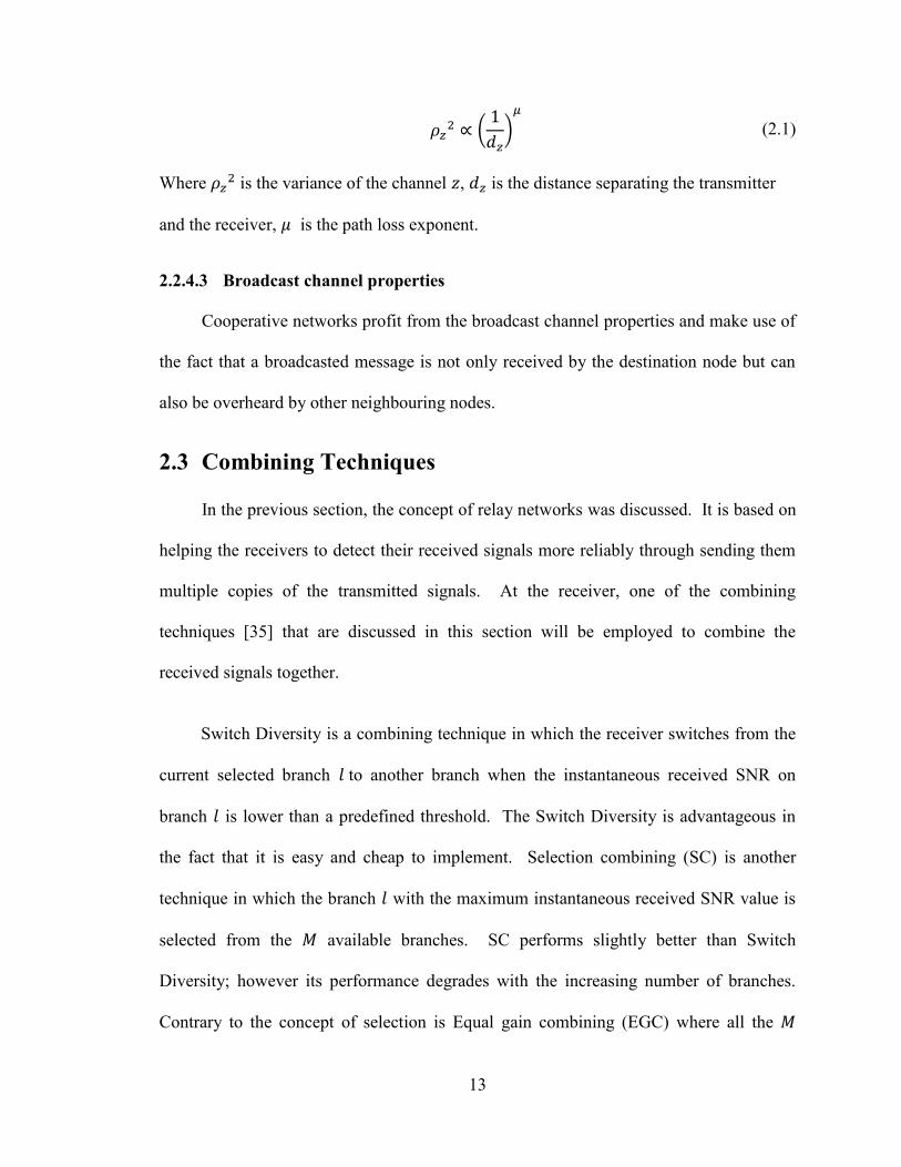
Where is the variance of the channel , is the distance separating the transmitter
and the receiver, is the path loss exponent.
2.2.4.3 Broadcast channel properties
Cooperative networks profit from the broadcast channel properties and make use of
the fact that a broadcasted message is not only received by the destination node but can
also be overheard by other neighbouring nodes.
2.3 Combining Techniques
In the previous section, the concept of relay networks was discussed. It is based on
helping the receivers to detect their received signals more reliably through sending them
multiple copies of the transmitted signals. At the receiver, one of the combining
techniques [35] that are discussed in this section will be employed to combine the
received signals together.
Switch Diversity is a combining technique in which the receiver switches from the
current selected branch to another branch when the instantaneous received SNR on
branch is lower than a predefined threshold. The Switch Diversity is advantageous in
the fact that it is easy and cheap to implement. Selection combining (SC) is another
technique in which the branch with the maximum instantaneous received SNR value is
selected from the available branches. SC performs slightly better than Switch
Diversity; however its performance degrades with the increasing number of branches.
Contrary to the concept of selection is Equal gain combining (EGC) where all the
14
available branches are simply co-phased and then summed. Finally, Maximal Ratio
combining (MRC) comes as the optimum combining technique in terms of performance.
In MRC, each of the signals is weighted proportionally to its channel quality, co-
phased then all signals are summed. This technique maximizes the instantaneous SNR at
the combiner’s output.
2.4 Drawbacks of cooperative networks
The cooperative networks have proved to be one of the very promising methods
in mitigating channel fading [15] [16] [17]. However cooperative networks have two
major drawbacks. The first drawback that cooperative networks suffer from is the error
propagation resulting from erroneous detection at the relay. Such error propagation
results in a degradation of the overall system’s performance. Another disadvantage
that cooperative networks experiences is its need for extra bandwidth. As can be seen
from Figure 2.1, relay networks require more time slots to transmit their data than the
traditional communication networks. Due to the operating nature of the relay nodes,
they can only operate in half duplex mode, which means that they can either transmit
or receive signals at one time. In a uni-directional cooperative network scenario;
where the relay assists the source in transmitting its data to the destination; this implies
that a whole transmission will require two or more time slots. In a bi-directional
scheme (Figure 2.2); where both nodes are exchanging data with the help of the relay;
four or more time slots are needed. In the sections to follow, discussions on each of
these drawbacks and the work done to overcome each of these disadvantages is
presented.
15
2.4.1 Mitigating error propagation in cooperative networks
As mentioned earlier, forwarding schemes in cooperative networks include Decode
and Forward (DF), Amplify and Forward (AF) and others. In case of employing DF
scheme, when perfect channel and correct detection at the relay is assumed, the diversity
of the system is preserved. However, if erroneous detection at the relay occurs, the relay
forwards incorrect messages which results in error propagation and a degradation of the
system’s performance. Several studies have been proposed to remedy the causes of
degradation and control the propagation of the error at the relay. Several papers [20],
[33] and [41] have suggested employing a Signal to Noise Ratio (SNR) threshold at the
relay. If the SNR of the received signal at the relay is above a predetermined threshold,
then the relay can forward the received signal. Otherwise the relay remains silent.
Others suggested employing AF forwarding scheme when the relay can not detect the
message correctly at the relay and employing DF otherwise [42] [43]. Another employed
method to control error propagation is the use of Cyclic Redundancy Check (CRC). In
case the CRC check fails, the relay does not forward its decoded message. This method
was discussed in [19], [44] and others.
2.4.2 Throughput degradation in cooperative networks
Methods like Network Coding [1], [2], [45], [46] Superposition Coding [15],
[47] and multi-level modulations [48], [49] were proposed to solve the dilemma of
additional bandwidth resources. Network Coding was initially introduced in the field
of computer networks for routing purposes [1], [4], [50]. Recently it has been
recommended for the cooperative wireless networks due to its capabilities of
compensating for the extra bandwidth that cooperative networks require [51] [52] [53]
16
[54]. In [52], the authors employed Network Coding at the relay in a bi-directional
relaying scheme. Instead of a traditional 4-phase transmission scheme, the Network
Coding at the relay reduces the number of needed transmissions to 3-phase
transmissions. Thus, the system throughput is enhanced by up to 33%. In a different
scenario, a system consisting of two sources transmitting their data to a common
destination with the help of a relay was described by Larson et al. in [53]. In this
context, each source broadcasts its data, which is received by the relay and the
destination nodes. The relay combines the data from the two sources using Network
Coding and broadcasts the Log Likelihood Ratio (LLR) of the network coded message
to the destination. In addition, a comparison between the performance of NC and SPC
in an uplink scheme was proposed in [54]. It consisted of multiple users, multiple
relays and a Base Station. It was concluded that Network Coding performed better in
high rate regions.
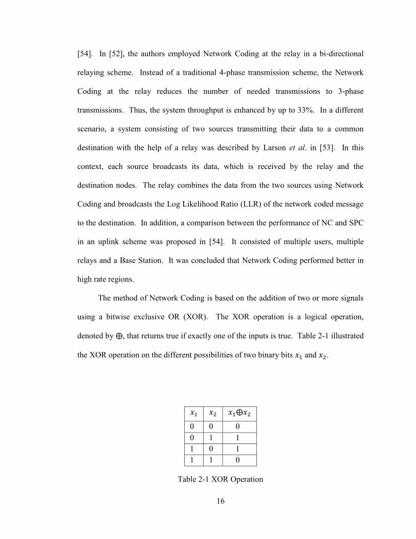
The method of Network Coding is based on the addition of two or more signals
using a bitwise exclusive OR (XOR). The XOR operation is a logical operation,
denoted by , that returns true if exactly one of the inputs is true. Table 2-1 illustrated
the XOR operation on the different possibilities of two binary bits and .
0 0 0
0 1 1
1 0 1
1 1 0
Table 2-1 XOR Operation
17
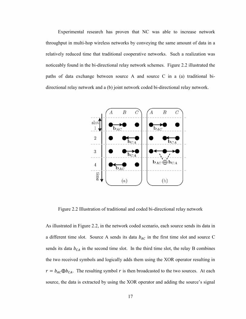
Experimental research has proven that NC was able to increase network
throughput in multi-hop wireless networks by conveying the same amount of data in a
relatively reduced time that traditional cooperative networks. Such a realization was
noticeably found in the bi-directional relay network schemes. Figure 2.2 illustrated the
paths of data exchange between source A and source C in a (a) traditional bi-
directional relay network and a (b) joint network coded bi-directional relay network.
Figure 2.2 Illustration of traditional and coded bi-directional relay network
As illustrated in Figure 2.2, in the network coded scenario, each source sends its data in
a different time slot. Source A sends its data in the first time slot and source C
sends its data in the second time slot. In the third time slot, the relay B combines
the two received symbols and logically adds them using the XOR operator resulting in
. The resulting symbol is then broadcasted to the two sources. At each
source, the data is extracted by using the XOR operator and adding the source’s signal
18
with the signal it has received from the relay B. For example, at source A, the
recovered signal is . In the same manner, the recovered
signal at source 2 is .
Several forwarding schemes were studied in the network coded bi-directional
cooperative networks schemes. Decode and Forward (DF) was discussed in [52], [46].
Amplify and Forward (AF) was studied in [55], [56]. De-noise and Forward (DNF)
was proposed and compared to DF and AF in [57]. In [57], the author concluded that
in noiseless channels, DNF and AF can achieve better throughput compared to DF
scheme. In addition, at low SNR, DNF has the best throughput of the three schemes.
However, as Network Coding has proven to be very promising in improving the
throughput of cooperative networks, it was discovered that such an achievement is only
limited to cooperative networks with symmetrical channels. In other words, in relay
networks, the rate of the better channel is limited by the rate of the poorer channel
when the channels are asymmetric. This has encouraged more research to find other
alternatives to be implemented in asymmetrical channels. In [58], a Joint SPC and NC
scheme was presented in an asymmetric channels bi-directional relay network scenario.
Employing SPC on top of the NC in this scenario enabled the user with the better
channel to make use of its advantageous channel by recovering extra information while
making sure that the user with the worse channel recovers its basic data. The same
concept was presented in [59] but for a multiple user exchange scenario.
Superposition Coding was first introduced by Cover in [5], [15]. Cover
examined the achievable joint rates in different broadcast channel schemes. He
19
concluded that “ high joint rates of transmission are best achieved by superimposing
high-rate and low-rate information rather than by using time-sharing” [5]. More
recently Superposition Coding was adopted in cooperative networks to overcome the
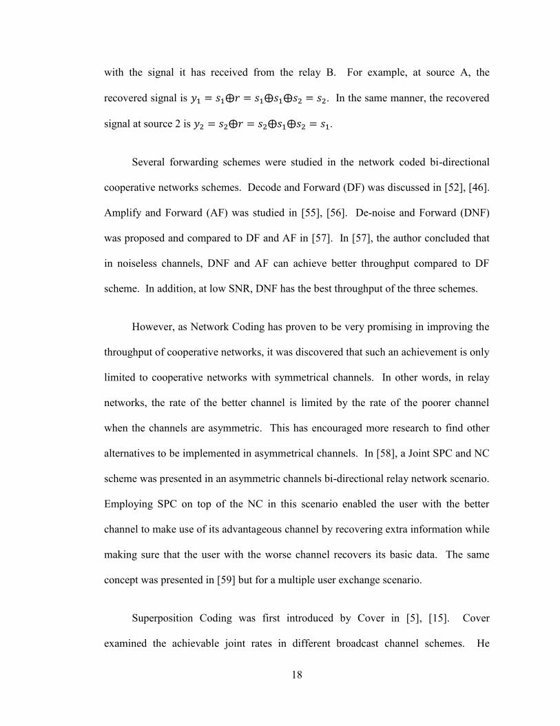
need of extra bandwidth. Superposition Coding was thoroughly studied in a three
nodes cooperative scheme [60], [61], [62], [63]. In this proposed scheme, two source
nodes, node A and node B cooperate together to deliver their information to a
destination node D. At the beginning of the transmission, node B broadcasts its data
that is received by node A. Node A then superposes node B data on its own data and
broadcasts the compound signal. Node B then receives the superimposed signal, where
it can extract node A signal since it knows its own signal. On its turn, node B then
adds together its own data and node A data using a different Superposition Coding
encoder depending on the a-priori information it has. Figure 2.3 illustrates the
proposed scheme.
Figure 2.3 Two nodes cooperation to deliver their data to a common destination using
SPC
20
Unidirectional relaying scheme using Superposition Coding at the source node
was proposed in [64], [65]. In these two papers, strategies for transmitting the intended
message using Superposition Coding are investigated. A proposal is presented
regarding dividing the data into two levels and transmitting them employing
superposition modulation. Power allocation at the source and the relay is studied to
optimize the performance of detection at the destination.
Due to the powerful capabilities of both Network Coding and Superposition
Coding on improving the throughput and the performance of cooperative networks,
more recent schemes involving joint Network Coding and Superposition Coding have
been proposed. Some work considered the two way relaying schemes [58], [6], [66]. In
the cited works, the case of asymmetric two way relay channels is considered. The
authors in [58] proposed employing Superposition Coding on top of Network Coding at
the relay. By employing such a technique, the user with the better channel will benefits
from its extra capacity by receiving the extra information embedded in the
Superposition Coding. Meanwhile, the user with the worse channel will still receive the
data resulting from the Network Coding. The authors have also included channel
capacity computations for both users. In [6], a comparison between the use of NC
versus the use SPC is presented in a two way wireless communication. It was proven
that SC performs better that NC in most of the cases in both scenarios of two and three
time slots transmission schemes. On a bigger scale, multiple nodes exchange in
cooperative networks using joint network-Superposition Coding was also discussed in
[59].
21
Joint network-Superposition Coding was also discussed in multicast cooperative
networks [7], [8], [31]. Signal multicast over asymmetric Rayleigh fading channels is
considered in [7], [8]. Superposition Coding is used on top of the Network Coding to
send extra data to users with good channel conditions. Results in these two papers
showed that additional performance gains were achieved in the proposed scheme when
compared to simple Network Coding schemes. In [31] comparison between
Superposition Coding and Network Coding with linearly independent global encoding
kernels in a multiple source multiple relay scheme is presented. Authors concluded that
finite field Network Coding has better performance than Superposition Coding in high
rate regions.
A joint Network Coding and Superposition Coding technique was described in
[59]. The authors compared this technique with two other techniques; pure time
division and pure Network Coding in two different relaying scenarios. They also
presented the achievable rate regions for every technique in every scenario and
concluded that the joint Network Coding and Superposition Coding technique was not
always superior and thus a combination of the three techniques was recommended.
In this section of the literature review, a brief summary of the methods used to
mitigate the drawbacks of cooperative networks were presented. The main drawbacks
mentioned were the error propagation resulting from erroneous detection at the relay
and the need for extra bandwidth compared to traditional transmission schemes. The
methods proposed along with the related discussions and the found results were
presented. In the coming section, the discussion continues on one of the methods more
recently introduced to cooperative networks, which is hierarchical modulation.
22
2.5 Hierarchical Modulation
Hierarchical modulation is a classification of the multi-level modulations. It was
originally introduced in the High Definition Television domain (HDTV) in 1993 [9].
The motive behind employing HM in HDTV systems is that receivers have different
channel fading conditions in broadcast channels. The use of multi-resolution
modulation allows the receivers located further away from the source or the ones that
experience bad channel conditions to receive at least a basic TV image quality.
Meanwhile, receivers with good channel quality can receive a HDTV signal quality.
Ten years later, hierarchical modulation was standardized in the digital video broadcast
(DVB) standards [49].
The concept of hierarchical modulation consists of transmitting multiple streams
of data with different protection simultaneously without any additional resources.
Hierarchical modulations are capable of prioritizing and dividing the data into different
classes of importance. This is useful in poor channel conditions, where the receiver
can recover the more protected classes (known as the coarse data) with a satisfactory
Bit Error Rate (BER), whereas the less protected classes (known as the enhancement
data), are only recovered in better channel conditions [67]. For example, in a 4/16
QAM hierarchical modulation, two 4-QAM are superposed on top of each other as
shown in Figure 2.4. The first 4-QAM, in this example referred to as “constellation
A”, is marked by big black dots. Each symbol in the “constellation A” is separated by a
distance of from its adjacent symbols. On top of each symbol of the “constellation
A” there is another 4-QAM constellation, denoted as “constellation B”. “Constellation
B” symbols are marked in Figure 2.4 by white small dots. Each symbol in the
23
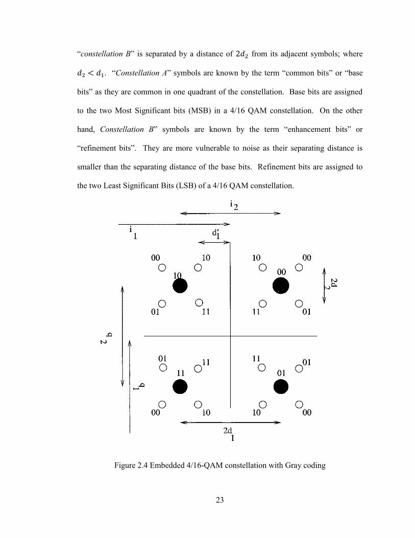
“constellation B” is separated by a distance of from its adjacent symbols; where
. “Constellation A” symbols are known by the term “common bits” or “base
bits” as they are common in one quadrant of the constellation. Base bits are assigned
to the two Most Significant bits (MSB) in a 4/16 QAM constellation. On the other
hand, Constellation B” symbols are known by the term “enhancement bits” or
“refinement bits”. They are more vulnerable to noise as their separating distance is
smaller than the separating distance of the base bits. Refinement bits are assigned to
the two Least Significant Bits (LSB) of a 4/16 QAM constellation.
Figure 2.4 Embedded 4/16-QAM constellation with Gray coding
24
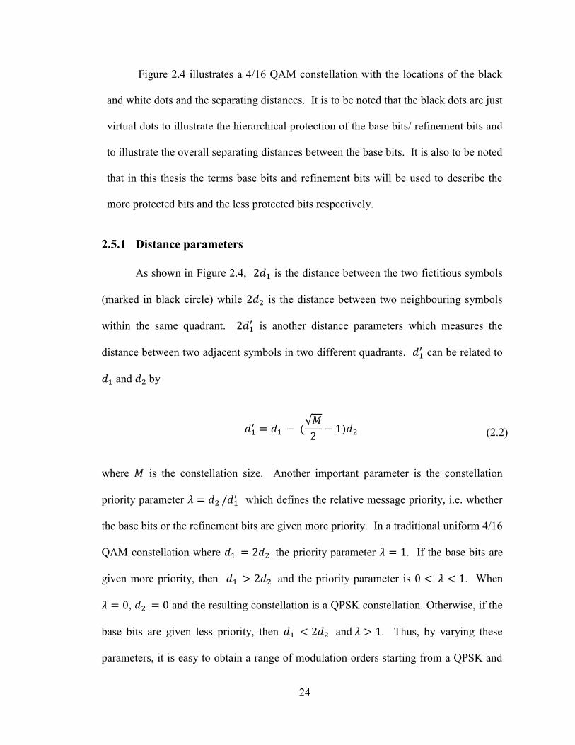
Figure 2.4 illustrates a 4/16 QAM constellation with the locations of the black
and white dots and the separating distances. It is to be noted that the black dots are just
virtual dots to illustrate the hierarchical protection of the base bits/ refinement bits and
to illustrate the overall separating distances between the base bits. It is also to be noted
that in this thesis the terms base bits and refinement bits will be used to describe the
more protected bits and the less protected bits respectively.
2.5.1 Distance parameters
As shown in Figure 2.4, is the distance between the two fictitious symbols
(marked in black circle) while is the distance between two neighbouring symbols
within the same quadrant. is another distance parameters which measures the
distance between two adjacent symbols in two different quadrants. can be related to
and by
√
(2.2)
where is the constellation size. Another important parameter is the constellation
priority parameter which defines the relative message priority, i.e. whether
the base bits or the refinement bits are given more priority. In a traditional uniform 4/16
QAM constellation where the priority parameter . If the base bits are
given more priority, then and the priority parameter is . When
, and the resulting constellation is a QPSK constellation. Otherwise, if the
base bits are given less priority, then and . Thus, by varying these
parameters, it is easy to obtain a range of modulation orders starting from a QPSK and
25
ending by a 16QAM with flexible streams prioritization. This makes hierarchical
modulation more powerful and more desirable that just simply adaptive modulation
technique.
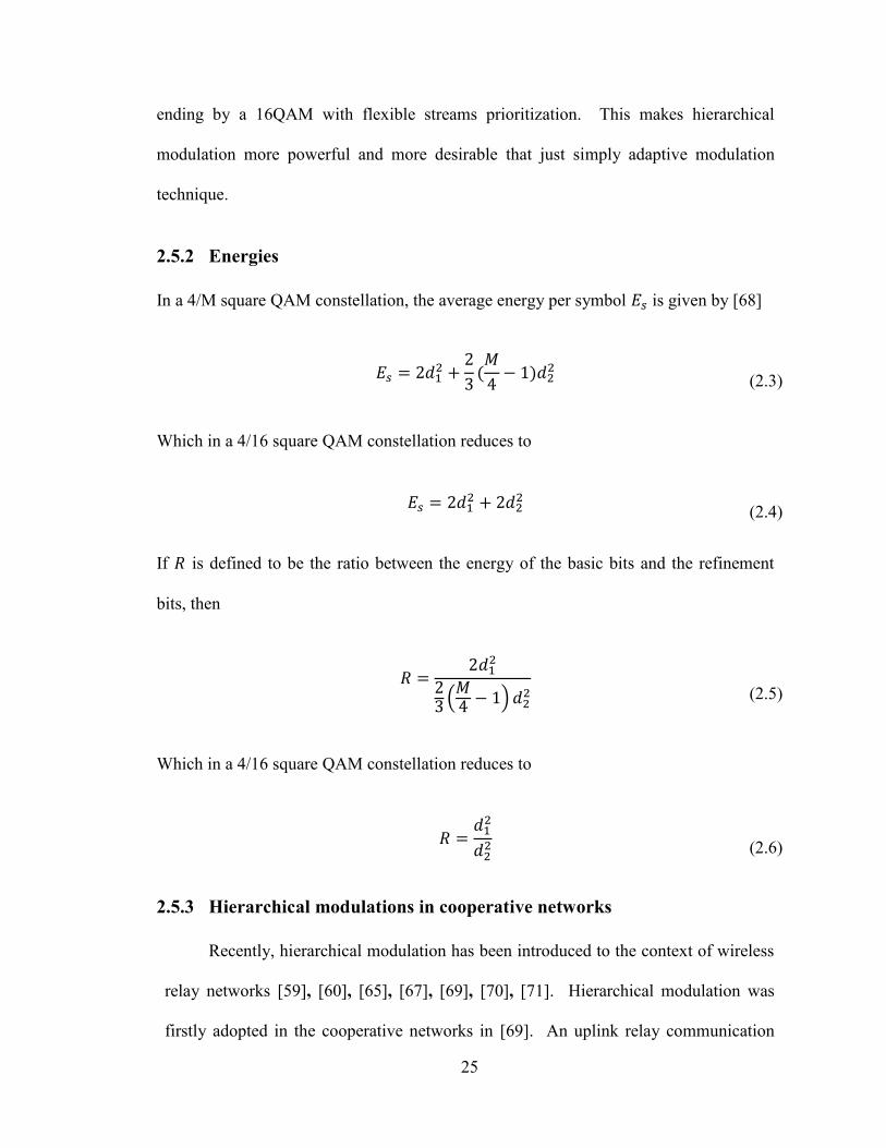
2.5.2 Energies
In a 4/M square QAM constellation, the average energy per symbol is given by [68]
(2.3)
Which in a 4/16 square QAM constellation reduces to
(2.4)
If is defined to be the ratio between the energy of the basic bits and the refinement
bits, then
(
)
(2.5)
Which in a 4/16 square QAM constellation reduces to
(2.6)
2.5.3 Hierarchical modulations in cooperative networks
Recently, hierarchical modulation has been introduced to the context of wireless
relay networks [59], [60], [65], [67], [69], [70], [71]. Hierarchical modulation was
firstly adopted in the cooperative networks in [69]. An uplink relay communication
26
system that uses channel coding was implemented, where in the first time slot the
source sends modulated and encoded data to both the relay and the destination. The
data are modulated at the source using hierarchical modulation, where the coarse data
are received by both the relay and the destination while the enhancement data is
received only by the relay. In the second time slot, the relay then sends additional
redundancy bits to the destination. Some other papers proposed hierarchical
modulation in order to solve the drawback problem of Network Coding in asymmetric
channels [67]. The problem is emphasized in wireless multicast networks, when the
data rate of network coded packets must be selected according to the worst channel
condition to ensure a reliable multicast. Such a constraint reduces the gain of the
Network Coding. In [67] a combined hierarchical modulation and Network Coding
algorithm which is known as hierarchically modulated Network Coding, was proposed
to accomplish spectral efficiency. Hierarchical modulation was used at user ‘A’, where
its protected data was received by the relay and user ‘B’. Meanwhile the relay
recovered the less protected data and combined it with user ‘B’ data using network
coding. The results of this scheme were compared to direct transmission, bidirectional
Network Coding and coded bidirectional relay. The proposed scheme was proven to
have a significantly improved BER.
In another network scenario, where receivers were grouped according to the
quality of their receptions, hierarchical modulation was applied in order to classify the
transmitted data according to each group reception’s quality [71]. In the same context,
a multiple relay scheme was presented in [70]. In the presented scheme, the source
modulated its signal using a hierarchical 16 QAM, where the data is received by the
27
relays and the destination. According to the CRC check at the relay, the relay re-
modulates its received data using the appropriate modulation technique that will
improve the system throughput. Non-uniform hierarchical modulation had also been
studied in relay networks and it successfully outperformed its uniform counterpart as
explained in [72]. Furthermore, an explicit closed form for the BER was derived for
cooperative communication systems with hierarchical modulation over Additive White
Gaussian Noise (AWGN) channels and Rayleigh fading channels in [10]. This BER
derivation was a function of the 16 QAM constellation’s distance parameters. In [73]
another model implemented a Signal to Noise Ratio (SNR) threshold at the relay in
order to decide whether to retransmit the received data or to remain silent while using
hierarchical modulation at the source to prioritize the different transmitted data.
Performance analyses of hierarchical modulation in several cooperative network
schemes were presented in [10], [11], [73].
In conclusion, the concept of hierarchical modulation was introduced in this
section. Examples of its important role in HDTV and cooperative network fields were
presented. The concept of classes’ protection in a hierarchical modulation was
explained and the respective energy of each group of protection was computed. A
review of the recent related work to hierarchical modulation in cooperative networks
was presented. In the coming section, a background along with a brief literature
review regarding Turbo codes is presented. A focus on the literature regarding Turbo
codes in cooperative networks with the aid of hierarchical modulation is presented.
28
2.6 Error Correcting Codes: Turbo Codes
Turbo codes are one of the most powerful codes that are widely used in the field
of satellite and wireless communications. They were first introduced in 1993 by
Berrou, Glavieux and Thitimajshima [74] [75]. Berrou et al. developed a Parallel
Concatenated Convolutional Codes (PCCC) using Recursive Systematic Convolutional
(RSC) codes with rate ⁄ . Using an interleaver with size N=65,536, they
achieved a BER of at 0.7 dB in an AWGN channel using Binary Phase Shift
Keying (BPSK) modulation after 18 iterations. In the following years, several
researches, developments, applications and tutorials on Turbo codes have been done.
Several papers analyzed the performance of Turbo codes with different settings (such
as rate, constraint length, interleaver size…etc) [76] [77] [78]. Tutorials on the
principles and applications of Turbo codes were described in details in [79] [80] [81]
[82] [83]. Developments of classes of Turbo codes such as Block Turbo codes and
Non-Binary Turbo codes took place in [84] [85] [86] [87] [88]. Major applications of
Turbo codes such as deep space, satellite communications and cellular networks were
presented in [81] [89].
Turbo codes are a high performance class of Forward Error Correcting codes
(FEC). The Turbo encoder is primarily composed of two recursive systematic
convolutional (RSC) codes concatenated in parallel and separated by an interleaver. On
the other end, the Turbo decoder is composed of two iterative Soft Input Soft Output
(SISO) decoders that exchange their output data to reach an accurate decision on the
received data. Each SISO decoder utilizes the Maximum a posteriori (MAP) algorithm
29
to decode its data. In the following section we will discuss the concept of Forward Error
Correcting codes, the composition of Turbo codes encoder and decoder and will briefly
discuss the MAP algorithm.
2.6.1 Forward Error Correction Codes
In general, Error Control Coding is divided in two subclasses; Automatic Repeat
Request (ARQ) and Forward Error Correction (FEC) codes. An ARQ code detects the
presence of errors and asks for a retransmission of the packets in error. An FEC detects
and as much as possible correct the messages in error. ARQ requires less bandwidth as
it doesn’t require any redundancy; however it is not practical in real time application
because of its latency which makes FEC more suitable for such applications. FEC is
divided in two main subclasses; block codes and convolutional codes. The main
difference between block codes and convolutional codes lies in the encoding scheme.
Block codes encode their message block by block. They take as input a symbol block
and encode it into an symbol codeword, where and are fixed and relatively long.
On the other hand, Convolutional codes keep encoding the data continuously avoiding
fixed packet size where and are small. We will focus more on the structure of
Convolutional Codes as they are the main components of Turbo codes.
2.6.2 On Convolutional encoders
A Convolutional encoder is illustrated in Figure 2.5. As shown in the Figure, a
convolutional encoder is composed of a number of shift registers m, that have as input
stream , and as output branches denoted by . Each is a specific modulo-2
addition of two or more of the data bits in the shift registers. The number of bits in the
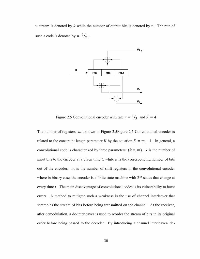
30
stream is denoted by while the number of output bits is denoted by . The rate of
such a code is denoted by ⁄ .
Figure 2.5 Convolutional encoder with rate ⁄ and
The number of registers , shown in Figure 2.5Figure 2.5 Convolutional encoder is
related to the constraint length parameter by the equation . In general, a
convolutional code is characterized by three parameters: . is the number of
input bits to the encoder at a given time , while is the corresponding number of bits
out of the encoder. is the number of shift registers in the convolutional encoder
where in binary case, the encoder is a finite state machine with states that change at
every time . The main disadvantage of convolutional codes is its vulnerability to burst
errors. A method to mitigate such a weakness is the use of channel interleaver that
scrambles the stream of bits before being transmitted on the channel. At the receiver,
after demodulation, a de-interleaver is used to reorder the stream of bits in its original
order before being passed to the decoder. By introducing a channel interleaver/ de-
m1 m0 m-1U
V0
V1
V2
31
interleaver to the system, the burst errors are spread out and appear independent to the
decoder [90]. For more details on convolution codes, the reader is referred to [91].
2.6.3 Turbo encoder
A Turbo encoder is the parallel concatenation of two recursive systematic
convolutional (RSC) codes separated by an interleaver. The upper encoder receives the
stream while the lower interleaver receives an interleaved version of denoted by .
The interleaver is a pseudo random interleaver. The interleaver permutates the bits
block by block; it takes bits at a time and interleaves them. Since the two encoders are
identical, the systematic bits of the second encoder are omitted. Meanwhile, the parity
bits of both encoders are transmitted. The code rate of a Turbo code constructed from
two parallel concatenated RSC each of rate one half is of rate one third. For higher code
rates, puncturing can be employed. An example of a Turbo encoder is presented in
Figure 2.6.
32
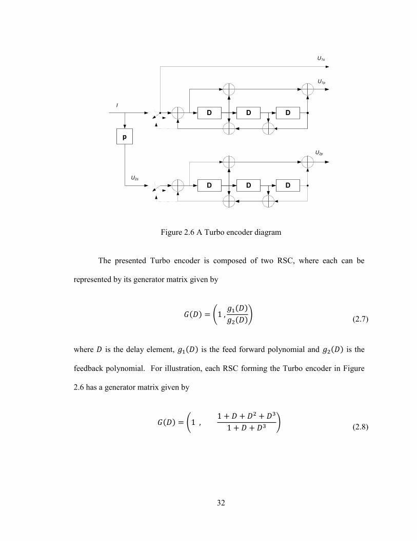
Figure 2.6 A Turbo encoder diagram
The presented Turbo encoder is composed of two RSC, where each can be
represented by its generator matrix given by
(
)
(2.7)
where is the delay element, is the feed forward polynomial and is the
feedback polynomial. For illustration, each RSC forming the Turbo encoder in Figure
2.6 has a generator matrix given by
(
)
(2.8)
D D D
p
D D D
I
U2s
U1s
U1p
U2p
33
This expression can also be written in octal format using the octal representation of the
feedback and feed forward polynomials as in . The octal representation of
the generator polynomials of the RSC in Figure 2.6 is .
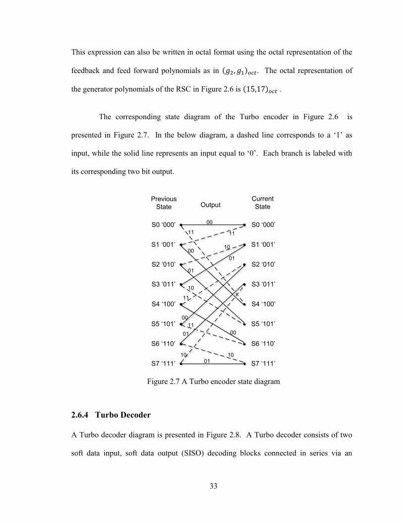
The corresponding state diagram of the Turbo encoder in Figure 2.6 is
presented in Figure 2.7. In the below diagram, a dashed line corresponds to a ‘1’ as
input, while the solid line represents an input equal to ‘0’. Each branch is labeled with
its corresponding two bit output.
S0 ‘000’
S1 ‘001’
S2 ‘010’
S3 ‘011’
S4 ‘100’
S5 ‘101’
S6 ‘110’
S7 ‘111’
S0 ‘000’
S1 ‘001’
S2 ‘010’
S3 ‘011’
S4 ‘100’
S5 ‘101’
S6 ‘110’
S7 ‘111’
00
00
00
00
11 11
11
11
10
10
1010
01
01
01
01
Previous
State
Current
StateOutput
Figure 2.7 A Turbo encoder state diagram
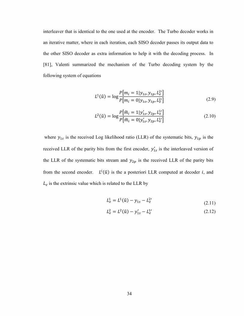
2.6.4 Turbo Decoder
A Turbo decoder diagram is presented in Figure 2.8. A Turbo decoder consists of two
soft data input, soft data output (SISO) decoding blocks connected in series via an
34
interleaver that is identical to the one used at the encoder. The Turbo decoder works in
an iterative matter, where in each iteration, each SISO decoder passes its output data to
the other SISO decoder as extra information to help it with the decoding process. In
[81], Valenti summarized the mechanism of the Turbo decoding system by the
following system of equations
[
]
[ ]
(2.9)
[
]
[
] (2.10)
where is the received Log likelihood ratio (LLR) of the systematic bits, is the
received LLR of the parity bits from the first encoder, is the interleaved version of
the LLR of the systematic bits stream and is the received LLR of the parity bits
from the second encoder. is the a posteriori LLR computed at decoder , and
is the extrinsic value which is related to the LLR by
(2.11)
(2.12)
35
Figure 2.8 Turbo Decoder Diagram
The ensemble of equations (2.9) to (2.12) is solved in an iterative manner as shown in
Figure 2.8. The two decoders keep passing their soft information to one another for a
predefined number of iterations. This procedure results in a refined estimate of the a
posteriori probability of the information bits. At the end of the final iteration, a hard
decision is made according to
{
(2.13)
where is the de-interleaved version of
2.6.5 SISO decoder
As mentioned in the previous section, a Turbo decoder consists of two soft data
input, soft data output (SISO) decoding blocks ,as shown in Figure 2.9 [92],connected in
series via an interleaver that is identical to the one used at the encoder. There are two
main inputs to the SISO decoder. The first input is the log likelihood ratio (LLR) of the
a priori probability of all information bits .
Decoder
#1
Decoder
#2
∑
∑
π
π
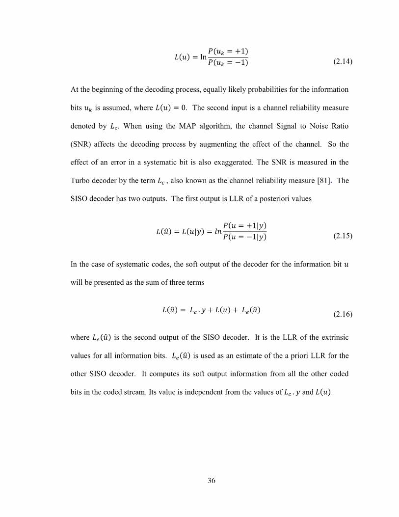
36
(2.14)
At the beginning of the decoding process, equally likely probabilities for the information
bits is assumed, where . The second input is a channel reliability measure
denoted by . When using the MAP algorithm, the channel Signal to Noise Ratio
(SNR) affects the decoding process by augmenting the effect of the channel. So the
effect of an error in a systematic bit is also exaggerated. The SNR is measured in the
Turbo decoder by the term , also known as the channel reliability measure [81]. The
SISO decoder has two outputs. The first output is LLR of a posteriori values
(2.15)
In the case of systematic codes, the soft output of the decoder for the information bit
will be presented as the sum of three terms
(2.16)
where is the second output of the SISO decoder. It is the LLR of the extrinsic
values for all information bits. is used as an estimate of the a priori LLR for the
other SISO decoder. It computes its soft output information from all the other coded
bits in the coded stream. Its value is independent from the values of and .
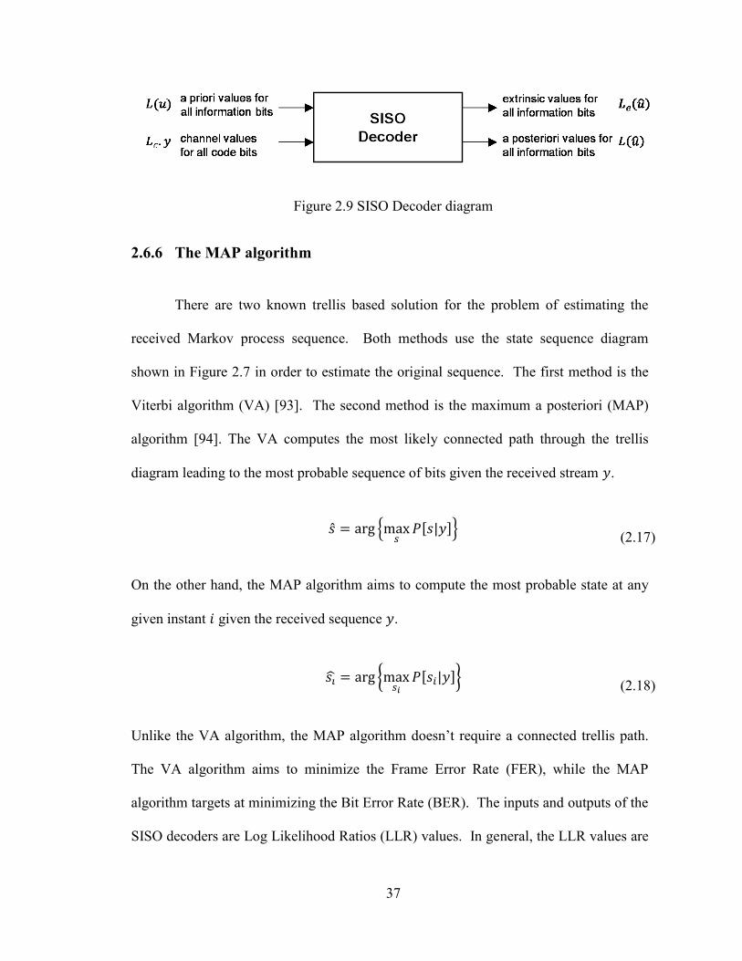
37
Figure 2.9 SISO Decoder diagram
2.6.6 The MAP algorithm
There are two known trellis based solution for the problem of estimating the
received Markov process sequence. Both methods use the state sequence diagram
shown in Figure 2.7 in order to estimate the original sequence. The first method is the
Viterbi algorithm (VA) [93]. The second method is the maximum a posteriori (MAP)
algorithm [94]. The VA computes the most likely connected path through the trellis
diagram leading to the most probable sequence of bits given the received stream .
{
[ ]} (2.17)
On the other hand, the MAP algorithm aims to compute the most probable state at any
given instant given the received sequence .
{
[ ]} (2.18)
Unlike the VA algorithm, the MAP algorithm doesn’t require a connected trellis path.
The VA algorithm aims to minimize the Frame Error Rate (FER), while the MAP
algorithm targets at minimizing the Bit Error Rate (BER). The inputs and outputs of the
SISO decoders are Log Likelihood Ratios (LLR) values. In general, the LLR values are
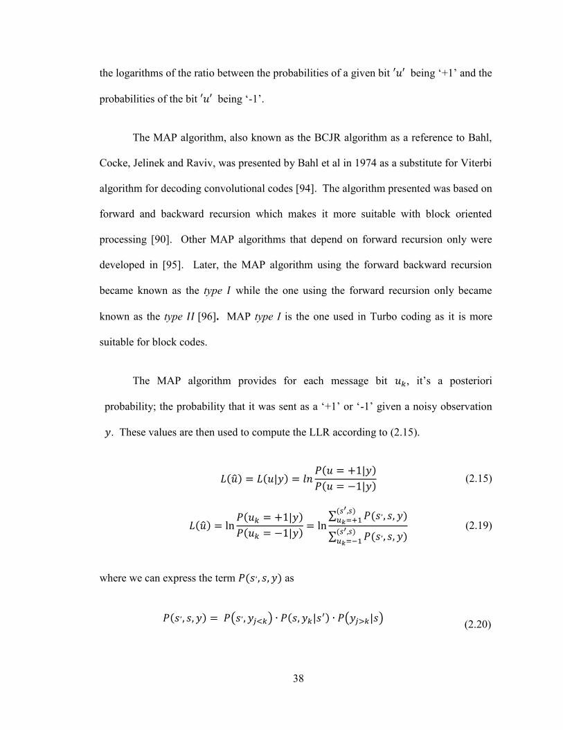
38
the logarithms of the ratio between the probabilities of a given bit being ‘+1’ and the
probabilities of the bit being ‘-1’.
The MAP algorithm, also known as the BCJR algorithm as a reference to Bahl,
Cocke, Jelinek and Raviv, was presented by Bahl et al in 1974 as a substitute for Viterbi
algorithm for decoding convolutional codes [94]. The algorithm presented was based on
forward and backward recursion which makes it more suitable with block oriented
processing [90]. Other MAP algorithms that depend on forward recursion only were
developed in [95]. Later, the MAP algorithm using the forward backward recursion
became known as the type while the one using the forward recursion only became
known as the type [96]. MAP type I is the one used in Turbo coding as it is more
suitable for block codes.
The MAP algorithm provides for each message bit , it’s a posteriori
probability; the probability that it was sent as a ‘+1’ or ‘-1’ given a noisy observation
. These values are then used to compute the LLR according to (2.15).
(2.15)
∑
∑
(2.19)
where we can express the term as
( ) ( )
(2.20)
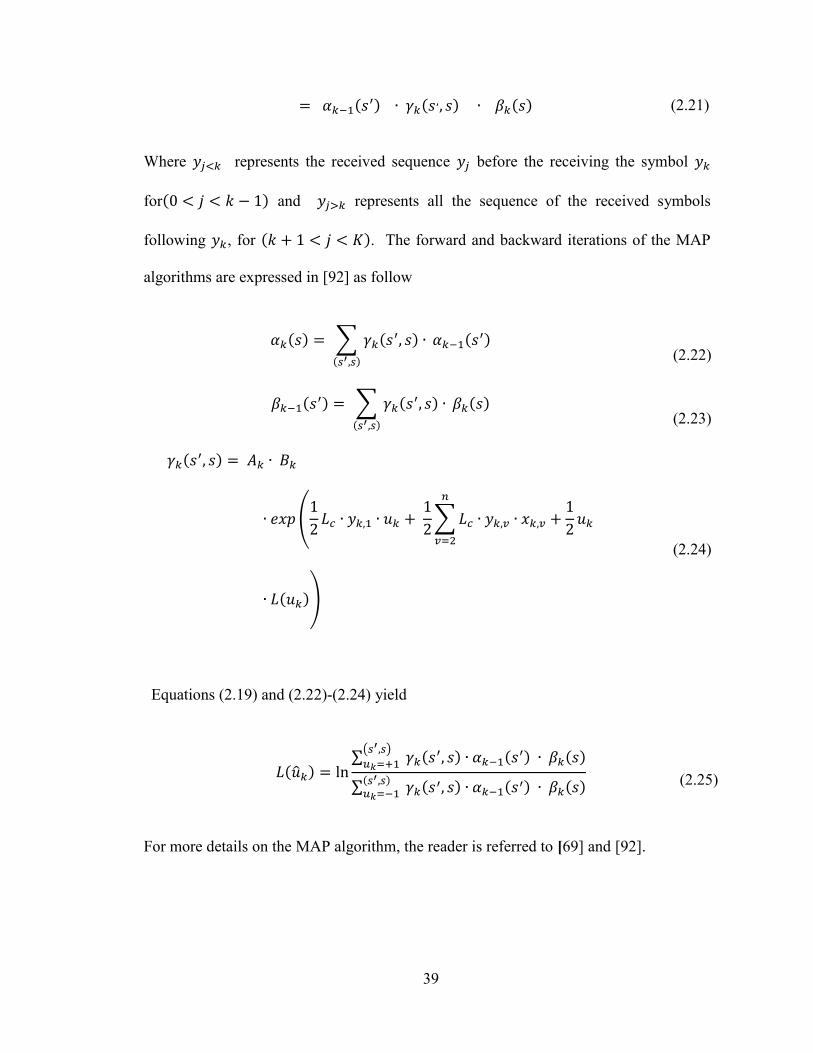
39
(2.21)
Where represents the received sequence before the receiving the symbol
for and represents all the sequence of the received symbols
following , for . The forward and backward iterations of the MAP
algorithms are expressed in [92] as follow
∑
(2.22)
∑
(2.23)
(
∑
)
(2.24)
Equations (2.19) and (2.22)-(2.24) yield
∑
( )
∑
(2.25)
For more details on the MAP algorithm, the reader is referred to [69] and [92].
40
2.6.7 Suboptimal algorithms
As mentioned before, the MAP algorithm is optimum for estimating the outputs
of a Markov process [92]. However, the MAP algorithm requires a lot of complex
computations that include non-linear functions and various additions and multiplications
which makes it unpractical to implement. It also suffers round off errors resulting from
the presentation of numerical values with finite precision [90]. Other alternatives such
as Log Map and Max log Map algorithms were proposed while avoiding the complexity
of the MAP algorithm [97].
The main advantage of employing the Log MAP algorithm or the Max Log MAP
is that the multiplication in the MAP algorithm becomes and addition in the log domain.
According to the Jacobian algorithm, the addition in the log domain is performed as
follow:
{ }
(2.26)
Equation (2.26) implies that the addition in the log domain is basically the summation of
the maximization operation and a correction function . In the case where and
are different, the correction function tends to be close to zero. In such scenario, it
is safe to imply that
(2.27)
The Log MAP and the Max Log MAP as mentioned earlier both compute the
multiplications as additions in the log domain. The Max Log MAP uses the

41
approximation in equation (2.27) while the Log MAP uses the refined function with the
correction function as in equation (2.26).
2.6.8 Turbo Codes and 16-QAM modulation
Even though binary Turbo codes can achieve a significant amount of coding gain,
they are not bandwidth efficient unless they are highly punctured. One of the methods
adopted to improve the bandwidth efficiency is the use of high order modulation. This
has made it interesting to examine the behavior of employing high order modulation with
Turbo codes. In this section, a survey on the previous work on Turbo codes and 16 QAM
modulation is presented.
The concept of employing high order modulation with Turbo codes was first
introduced in [98]. In this paper, Berou et al. proved that this joint scheme achieved a
considerable coding gain both on Gaussian and Rayleigh channels. In both channel
environments; the Gaussian channel and the Rayleigh fading channel; the described
scheme outperformed a 64-state trellis-coded modulation (TCM).
In [99], a joint 16-QAM modulation and binary Turbo codes were employed for
phase recovery. The soft bit data was computed at the 16QAM demodulator and used as
input to the Turbo decoder. The output of the Turbo decoder was then passed to the
phase recovery part to implement iterative Maximum Likelihood (ML) evaluation of the
carrier phase error. Meanwhile, the mapping of systematic bits and parity bits in a
16QAM modulation was examined in [100]. The authors used two modulation schemes;
8PSK and 16QAM; and compared them. It was concluded that mapping the systematic
bits to be more protected has led to an enhancement in the BER threshold. On the other
42
hand, mapping the parity bits to the more protected bits of the high order modulation
resulted in an improved error floor performance on the expense of slight degradation of
the BER threshold. In [101], a special non uniform 16QAM modulation was employed to
map the systematic and parity bits of a Turbo encoder. The motive behind this mapping
was to reduce the gap between the Shannon capacity limit and the performance of Turbo
codes at high SNR. The proposed mapping consisted of shaping the constellation’s
signals in a way that the constellation itself had a “Gaussian like distribution”. This
‘Gaussian like’ shaping had relatively more low energy signals compared to the uniform
constellation. This resulted in lower average symbol energy for fixed distance
constellations. Such a scheme can be beneficial in Satellite channel environment, as low
energy signals are less vulnerable to High Power Amplifiers (HPA) distortion. In
addition, a new iterative de-mapping and decoding scheme was proposed. The authors
employed an additional soft de-mapper between the two SISO decoders to improve the
channel estimation at the second decoder. Performance of the system employing this
extra de-mapper resulted in a gain of 0.9 dB at 10-5
over linear channels and 1.2dB over
non-linear channels.
A study on the design and performance of Unequal Error Protection (UEP) Turbo
coded modulation scheme was presented in [102]. The system presented involved
multiple streams with different importance to be sent on a wireless channel, using Turbo
coding. The study’s goal was to achieve UEP through three different scenarios. The first
scenario was to achieve Unequal Error Protection by employing non-uniform puncturing
after encoding the input stream. The non-uniform puncturing was designed in a way to
apply more puncturing to the less important data. The second method was to achieve
43
UEP by mapping the bits of the most important data to the base bits in a multi-resolution
modulation while mapping the least important stream bits to the refinement bits of the
same modulation. Finally, the third method was a combination of the first two methods.
They concluded that all presented schemes achieved high performance gains for the
important streams. Such a gain could not be accomplished using the traditional coded
modulation. They also concluded that the performance of the third method has the best
performance of the three methods.
Improving the system’s BER through adjusting the constellation’s symbol energy
was employed in [103]. The authors employed different symbol energy and examined
the results in different scenarios. However, no information on the channel condition or
the kind of Turbo encoder employed was provided. Another scheme was employed in
[104] where exchange between the 16QAM demodulator output and the Turbo decoder
data takes place in order to improve the accuracy of the decision. They concluded that
one iteration between the demodulator and the Turbo decoder is enough to improve the
system’s performance. However, regular iterations inside the Turbo decoder continue to
take place. Different values for the hierarchical 16QAM’s priority factor were employed
showing the different BER of base bits and refinement bits corresponding to each value.
44
Chapter Three
System Model 3.
3.1 Overview
In this chapter, the proposed system is presented and examined in details. The
main constituting nodes of the system are a Base Station ( ) and two User-Ends
and . In the presented downlink system, the aims at transmitting two different
streams of data to these two User-Ends simultaneously. Instead of sending each user’s
data on a different time slot, the concatenates the two streams of data and modulates
them by employing a 4/16-QAM hierarchical modulation. In one transmission, the
sends one ‘four bits symbol’ where two bits are destined to and two other bits are
destined to . Using a high order modulation like a 4/16 QAM results in time saving.
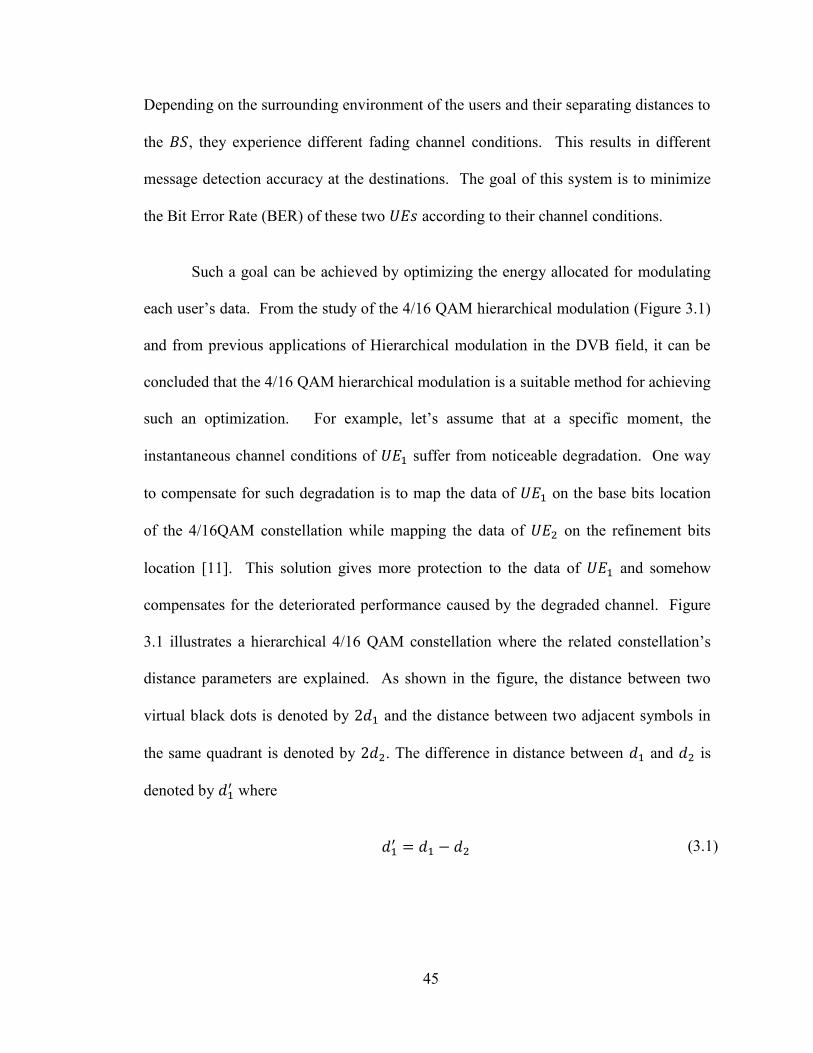
45
Depending on the surrounding environment of the users and their separating distances to
the , they experience different fading channel conditions. This results in different
message detection accuracy at the destinations. The goal of this system is to minimize
the Bit Error Rate (BER) of these two according to their channel conditions.
Such a goal can be achieved by optimizing the energy allocated for modulating
each user’s data. From the study of the 4/16 QAM hierarchical modulation (Figure 3.1)
and from previous applications of Hierarchical modulation in the DVB field, it can be
concluded that the 4/16 QAM hierarchical modulation is a suitable method for achieving
such an optimization. For example, let’s assume that at a specific moment, the
instantaneous channel conditions of suffer from noticeable degradation. One way
to compensate for such degradation is to map the data of on the base bits location
of the 4/16QAM constellation while mapping the data of on the refinement bits
location [11]. This solution gives more protection to the data of and somehow
compensates for the deteriorated performance caused by the degraded channel. Figure
3.1 illustrates a hierarchical 4/16 QAM constellation where the related constellation’s
distance parameters are explained. As shown in the figure, the distance between two
virtual black dots is denoted by and the distance between two adjacent symbols in
the same quadrant is denoted by . The difference in distance between and is
denoted by where
(3.1)
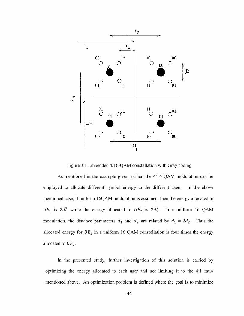
46
Figure 3.1 Embedded 4/16-QAM constellation with Gray coding
As mentioned in the example given earlier, the 4/16 QAM modulation can be
employed to allocate different symbol energy to the different users. In the above
mentioned case, if uniform 16QAM modulation is assumed, then the energy allocated to
is while the energy allocated to is
. In a uniform 16 QAM
modulation, the distance parameters and are related by . Thus the
allocated energy for in a uniform 16 QAM constellation is four times the energy
allocated to .
In the presented study, further investigation of this solution is carried by
optimizing the energy allocated to each user and not limiting it to the 4:1 ratio
mentioned above. An optimization problem is defined where the goal is to minimize
47
the summation of the base bits BER and the refinement bits BER in terms of the
distance parameters and . In other words, the general optimization problem can
be expressed as
{ }
{ √
(
) (3.2)
where is the energy per symbol.
This research examines three different schemes; the direct transmission scheme,
the nodes cooperation scheme and the Turbo coded cooperative scheme. In the first two
schemes, the instantaneous BER of the base bits and the refinement bits are derived.
These derivations are used in computing the values of and to achieve optimal total
BER. Furthermore, a comparison between the average BER of each user in the
optimized modulation case and the uniform modulation case is presented. Later in the
results section, it will be shown that this optimization results in a noticeable
improvement in BER for both users. Moreover, the presented study is extended to
estimate sub-optimal constellation distance parameters for the Turbo coded cooperative
scheme from the un-coded cooperative scheme derivations. Simulation results show
that these parameters estimates still have a better performance than the parameters of a
uniform constellation. In the following subsections, each scheme is presented along
with its parameters and necessary derivations. Later in this study, results of each
scheme’s performance are examined.
48
3.2 Direct Transmission
In the case of direct transmission, the transmits two different streams of data to
two destinations without any external assistance from surrounding nodes. It does that
by combining these two streams employing a 4/16QAM constellation where two bits of
the four bits symbol are assigned to and the other two bits are assigned to .
and are located at distances and
respectively from the . It is
assumed that
. Thus, the channel condition of is generally more
favorable than that of . Hence, to insure acceptable performance at both users, the
BS will modulate ’s data to be the base bits while ’s data to be the refinement
bits.
The binary data stream destined to is denoted by and the binary data
stream destined to is denoted by . Each of these two streams is of length . At a
given time , where , the Base Station concatenates the two streams in a
manner that the four bits symbol at time will be represented as
[ ] (3.3)
The transmitted modulated symbol is chosen from the set of 16 available symbols, as
shown in Figure 3.1 so that the modulated symbol in terms of the constellation’s
distance parameters is in the form of
(3.4)
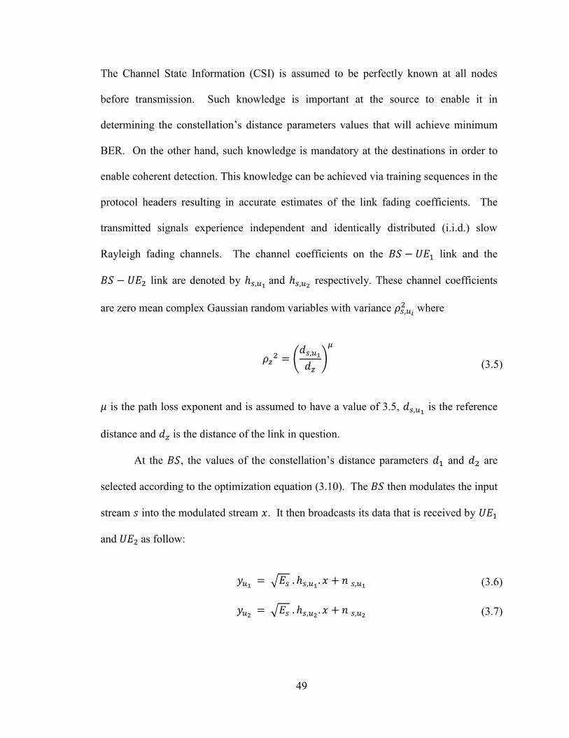
49
The Channel State Information (CSI) is assumed to be perfectly known at all nodes
before transmission. Such knowledge is important at the source to enable it in
determining the constellation’s distance parameters values that will achieve minimum
BER. On the other hand, such knowledge is mandatory at the destinations in order to
enable coherent detection. This knowledge can be achieved via training sequences in the
protocol headers resulting in accurate estimates of the link fading coefficients. The
transmitted signals experience independent and identically distributed (i.i.d.) slow
Rayleigh fading channels. The channel coefficients on the link and the
link are denoted by ℎ and ℎ
respectively. These channel coefficients
are zero mean complex Gaussian random variables with variance
where
(
)
(3.5)
is the path loss exponent and is assumed to have a value of 3.5, is the reference
distance and is the distance of the link in question.
At the , the values of the constellation’s distance parameters and are
selected according to the optimization equation (3.10). The then modulates the input
stream into the modulated stream . It then broadcasts its data that is received by
and as follow:
√ ℎ
(3.6)
√ ℎ
(3.7)
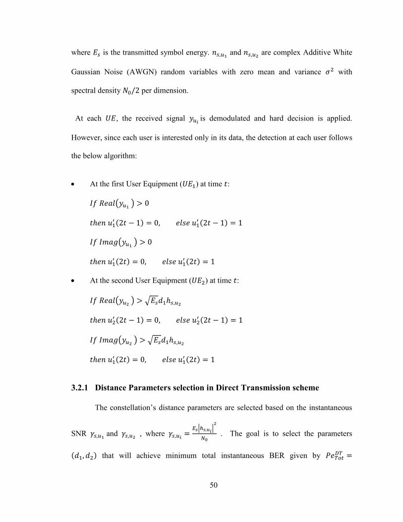
50
where is the transmitted symbol energy. and
are complex Additive White
Gaussian Noise (AWGN) random variables with zero mean and variance with
spectral density per dimension.
At each , the received signal is demodulated and hard decision is applied.
However, since each user is interested only in its data, the detection at each user follows
the below algorithm:
At the first User Equipment ( ) at time :
( )
ℎ
( )
ℎ
At the second User Equipment ( ) at time :
( ) √ ℎ
ℎ
( ) √ ℎ
ℎ
3.2.1 Distance Parameters selection in Direct Transmission scheme
The constellation’s distance parameters are selected based on the instantaneous
SNR and
, where
| |
. The goal is to select the parameters
that will achieve minimum total instantaneous BER given by
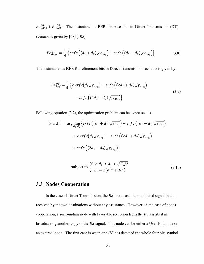
51
. The instantaneous BER for base bits in Direct Transmission (DT)
scenario is given by [68] [105]
{ ( √
) ( √ )} (3.8)
The instantaneous BER for refinement bits in Direct Transmission scenario is given by
{ ( √
) ( √ )
( √ )}
(3.9)
Following equation (3.2), the optimization problem can be expressed as
{ ( √ ) ( √
)
( √ ) ( √
)
( √ )}
{ √
(
) (3.10)
3.3 Nodes Cooperation
In the case of Direct Transmission, the broadcasts its modulated signal that is
received by the two destinations without any assistance. However, in the case of nodes
cooperation, a surrounding node with favorable reception from the assists it in
broadcasting another copy of the signal. This node can be either a User-End node or
an external node. The first case is when one has detected the whole four bits symbol
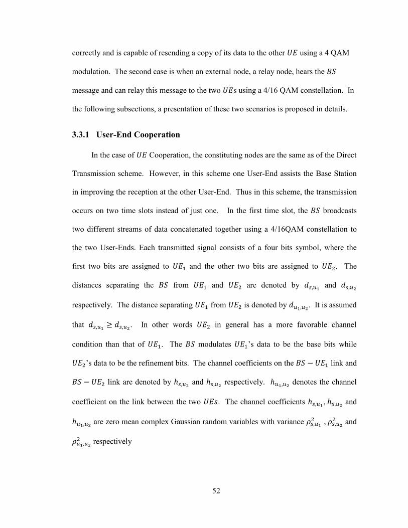
52
correctly and is capable of resending a copy of its data to the other using a 4 QAM
modulation. The second case is when an external node, a relay node, hears the
message and can relay this message to the two s using a 4/16 QAM constellation. In
the following subsections, a presentation of these two scenarios is proposed in details.
3.3.1 User-End Cooperation
In the case of Cooperation, the constituting nodes are the same as of the Direct
Transmission scheme. However, in this scheme one User-End assists the Base Station
in improving the reception at the other User-End. Thus in this scheme, the transmission
occurs on two time slots instead of just one. In the first time slot, the broadcasts
two different streams of data concatenated together using a 4/16QAM constellation to
the two User-Ends. Each transmitted signal consists of a four bits symbol, where the
first two bits are assigned to and the other two bits are assigned to . The
distances separating the from and are denoted by and
respectively. The distance separating from is denoted by . It is assumed
that
. In other words in general has a more favorable channel
condition than that of . The modulates ’s data to be the base bits while
’s data to be the refinement bits. The channel coefficients on the link and
link are denoted by ℎ and ℎ
respectively. ℎ denotes the channel
coefficient on the link between the two . The channel coefficients ℎ , ℎ
and
ℎ are zero mean complex Gaussian random variables with variance
, and
respectively
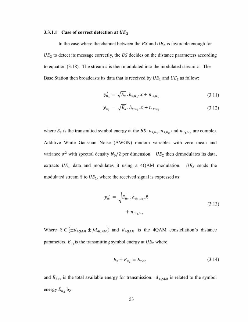
53
3.3.1.1 Case of correct detection at
In the case where the channel between the and is favorable enough for
to detect its message correctly, the decides on the distance parameters according
to equation (3.18). The stream is then modulated into the modulated stream . The
Base Station then broadcasts its data that is received by and as follow:
√ ℎ
(3.11)
√ ℎ
(3.12)
where is the transmitted symbol energy at the . ,
and are complex
Additive White Gaussian Noise (AWGN) random variables with zero mean and
variance with spectral density per dimension. then demodulates its data,
extracts data and modulates it using a 4QAM modulation. sends the
modulated stream to , where the received signal is expressed as:
√ ℎ
(3.13)
Where { } and is the 4QAM constellation’s distance
parameters. is the transmitting symbol energy at where
(3.14)
and is the total available energy for transmission. is related to the symbol
energy by
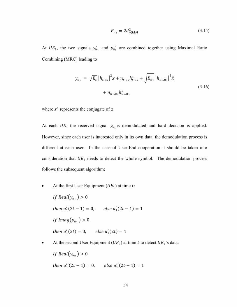
54
(3.15)
At , the two signals and
are combined together using Maximal Ratio
Combining (MRC) leading to
√ |ℎ
|
ℎ √
|ℎ |
ℎ
(3.16)
where represents the conjugate of .
At each , the received signal is demodulated and hard decision is applied.
However, since each user is interested only in its own data, the demodulation process is
different at each user. In the case of User-End cooperation it should be taken into
consideration that needs to detect the whole symbol. The demodulation process
follows the subsequent algorithm:
At the first User Equipment ( ) at time :
( )
ℎ
( )
ℎ
At the second User Equipment ( ) at time to detect ’s data:
( )
ℎ
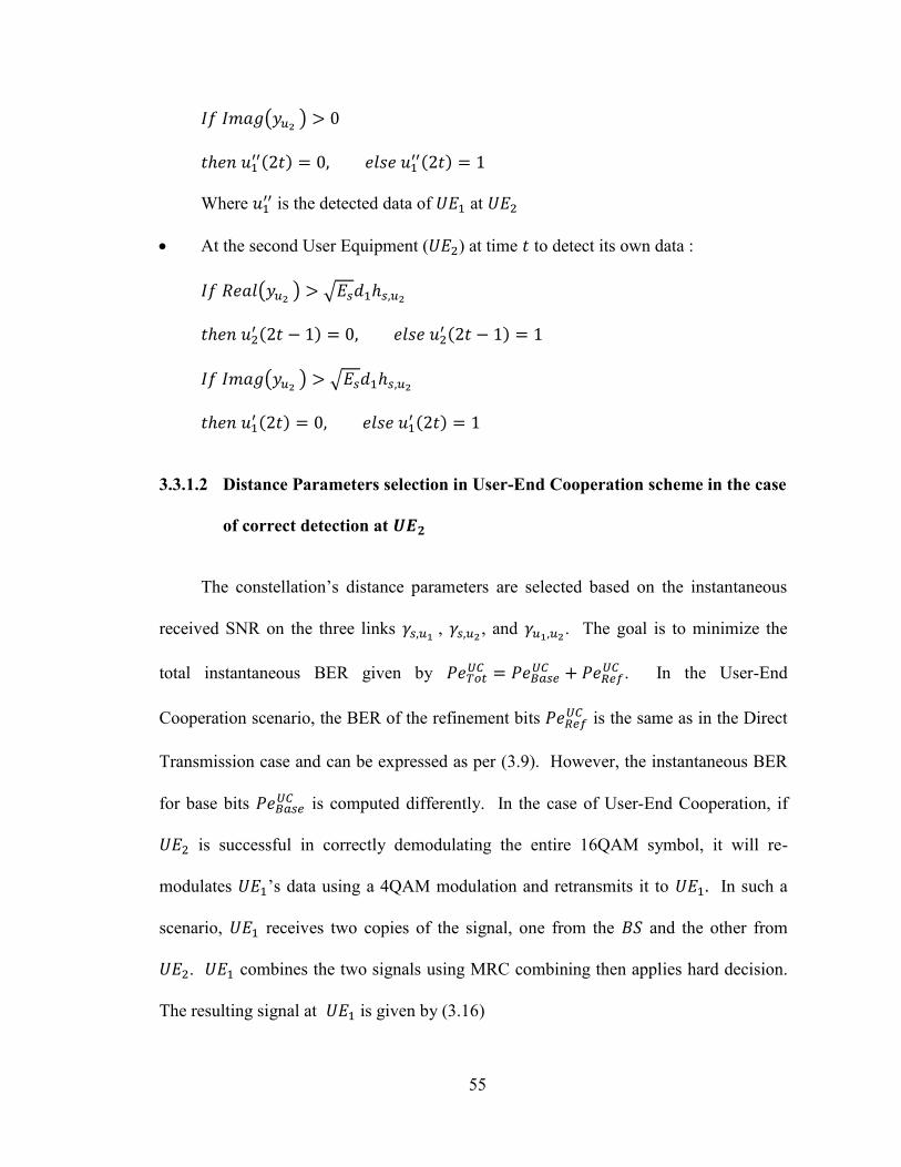
55
( )
ℎ
Where is the detected data of at
At the second User Equipment ( ) at time to detect its own data :
( ) √ ℎ
ℎ
( ) √ ℎ
ℎ
3.3.1.2 Distance Parameters selection in User-End Cooperation scheme in the case
of correct detection at
The constellation’s distance parameters are selected based on the instantaneous
received SNR on the three links ,
, and . The goal is to minimize the
total instantaneous BER given by
. In the User-End
Cooperation scenario, the BER of the refinement bits is the same as in the Direct
Transmission case and can be expressed as per (3.9). However, the instantaneous BER
for base bits is computed differently. In the case of User-End Cooperation, if
is successful in correctly demodulating the entire 16QAM symbol, it will re-
modulates ’s data using a 4QAM modulation and retransmits it to In such a
scenario, receives two copies of the signal, one from the and the other from
. combines the two signals using MRC combining then applies hard decision.
The resulting signal at is given by (3.16)
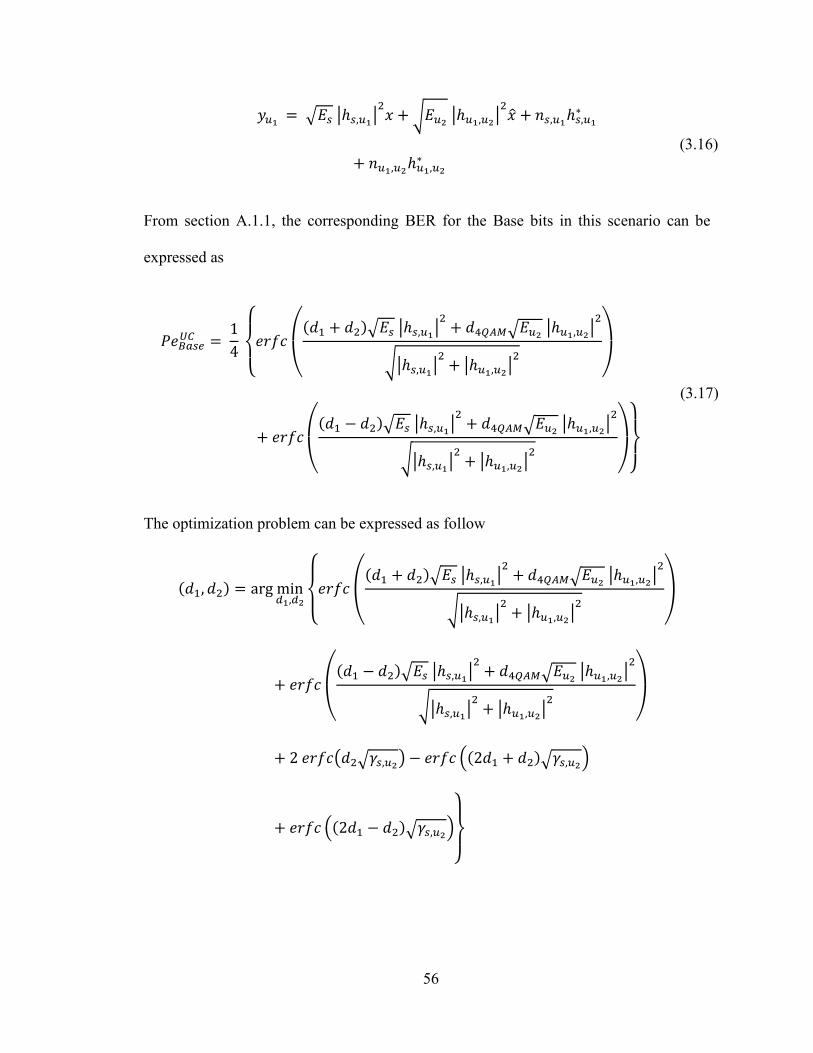
56
√ |ℎ
| √
|ℎ |
ℎ
ℎ
(3.16)
From section A.1.1, the corresponding BER for the Base bits in this scenario can be
expressed as
{
(
√ |ℎ
| √
|ℎ |
√|ℎ | |ℎ
|
)
(
√ |ℎ
| √
|ℎ |
√|ℎ | |ℎ
|
)
}
(3.17)
The optimization problem can be expressed as follow
{
(
√ |ℎ
| √
|ℎ |
√|ℎ | |ℎ
|
)
(
√ |ℎ
| √
|ℎ |
√|ℎ | |ℎ
|
)
( √ ) ( √
)
( √ )
}
57
{
√
(
)
(3.18)
3.3.1.3 Case of incorrect detection at
In the case where fails to detect its received signal, it will remain silent and
the system will act as a Direct Transmission system. In this case the distance parameters
selection will only take place at the BS and the selection will be handled in the same
manner as in section (3.2.1).
3.3.2 Relay Cooperation
In the case of Relay Cooperation, the constituting nodes are the same as of the
Direct Transmission scheme with the addition of a relaying node. As in the previous
mentioned schemes, the combines the two streams using a 4/16QAM modulation
then broadcasts the modulated signal. The base bits of the 16QAM constellation are
destined to whereas the refinement bits are assigned to . In the relay
cooperative scheme, the Relay listens to the message and forwards it employing
either Amplify and Forward (AF) technique or Decode and Forward (DF) technique.
After receiving the broadcasted copy from the Relay, each User-End combines the two
received signals coming from the and the Relay using Maximal Ratio Combining
(MRC) then applies hard decision on the resulting signal. Figure 3.2 Illustrates the
predicted relay cooperation system.
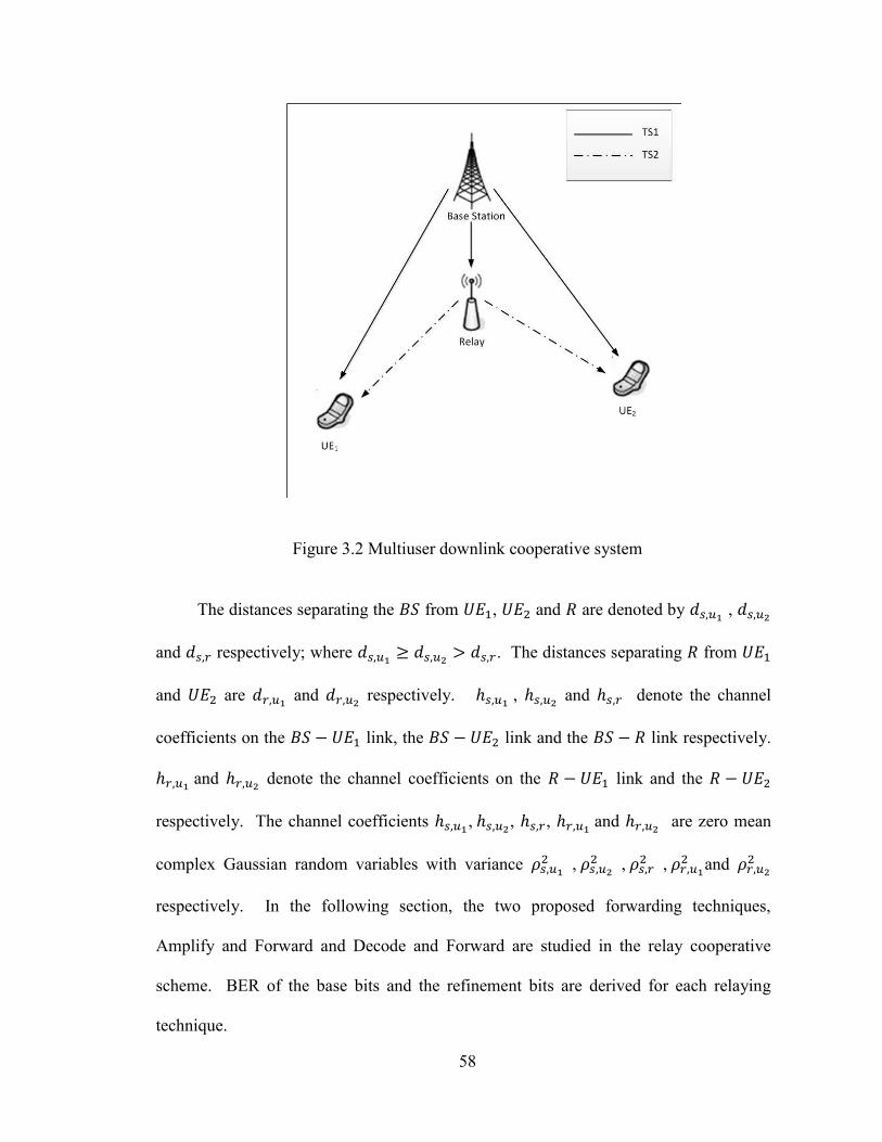
58
Figure 3.2 Multiuser downlink cooperative system
The distances separating the from , and are denoted by ,
and respectively; where
. The distances separating from
and are and
respectively. ℎ , ℎ
and ℎ denote the channel
coefficients on the link, the link and the link respectively.
ℎ and ℎ
denote the channel coefficients on the link and the
respectively. The channel coefficients ℎ , ℎ
, ℎ , ℎ and ℎ
are zero mean
complex Gaussian random variables with variance ,
, ,
and
respectively. In the following section, the two proposed forwarding techniques,
Amplify and Forward and Decode and Forward are studied in the relay cooperative
scheme. BER of the base bits and the refinement bits are derived for each relaying
technique.
59
3.3.2.1 Decode and Forward scenario
In the case of employing Decode and forward technique, the Relay detects and
decodes the data it receives from the . At the relay, a Cyclic Redundancy Check
(CRC) is applied in order to check the correctness of the detected data. If the Relay
succeeds in correctly decoding the received data, it re-encodes the stream of data and
sends it to the two . On the other hand, if the CRC check fails, the Relay node
remains silent and the two receive only one copy from the .
It is assumed that the channel is constant during the transmission of a whole
block of data. Before each block transmission, the first collects data on the channel
link connecting it to the Relay. From the collected data and from the derived probability
of error of the base bits and the refinement bits, the can guess whether the Relay will
be able to correctly decode the data it receives from the or not. Accordingly, the
modulates its data with the corresponding distance parameters that will ensure minimum
bit error at both .
For example, assuming that one block of transmission consists of equal streams of base
bits and refinements bits. Each of these two streams is of length bits. As mentioned
earlier, the relay will only forward its received data when this data is detected correctly.
Such data can be detected correctly when there exists a set of [ ] that satisfies the
following conditions
(3.19)
(3.20)
where
60
{ ( √ ) ( √ )}
(3.21)
{ ( √ ) ( √ )
( √ )}
(3.22)
In the case where there exists several sets of [ ] that satisfy the above mentioned
conditions then the set of [ ] that achieves the minimum total BER is chosen. If
such a set does not exist then the relay cannot correctly decode its received information.
Hence, the will modulate its data using a set of [ ] that will achieve optimum
performance through the direct transmission only, as per equation (3.10).
3.3.2.1.1 Case of Correct detection at relay
As mentioned in section 3.3.2.1, correct detection at the relay will occur when
there exists one or multiple sets of [ ] that satisfy conditions (3.19) and (3.20). If
there exists only one set of [ ], then the will use this set for its transmission.
However, if there exists multiple sets, then the will select the set that will minimize
the summation of equations (A.29) and (A.63) accordingly we get
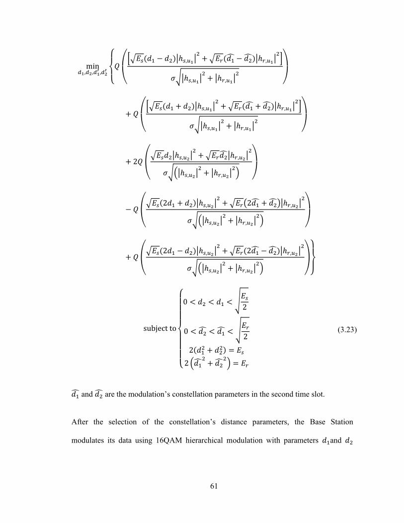
61
{
(
[√ |ℎ
| √ |ℎ
| ]
√|ℎ | |ℎ
|
)
(
[√ |ℎ
| √ |ℎ
| ]
√|ℎ | |ℎ
|
)
(
√ |ℎ
| √ |ℎ
|
√(|ℎ | |ℎ
| )
)
(
√ |ℎ
| √ ( )|ℎ
|
√(|ℎ | |ℎ
| )
)
(
√ |ℎ
| √ |ℎ
|
√(|ℎ | |ℎ
| )
)
}
{
√
√
(
)
(3.23)
and are the modulation’s constellation parameters in the second time slot.
After the selection of the constellation’s distance parameters, the Base Station
modulates its data using 16QAM hierarchical modulation with parameters and
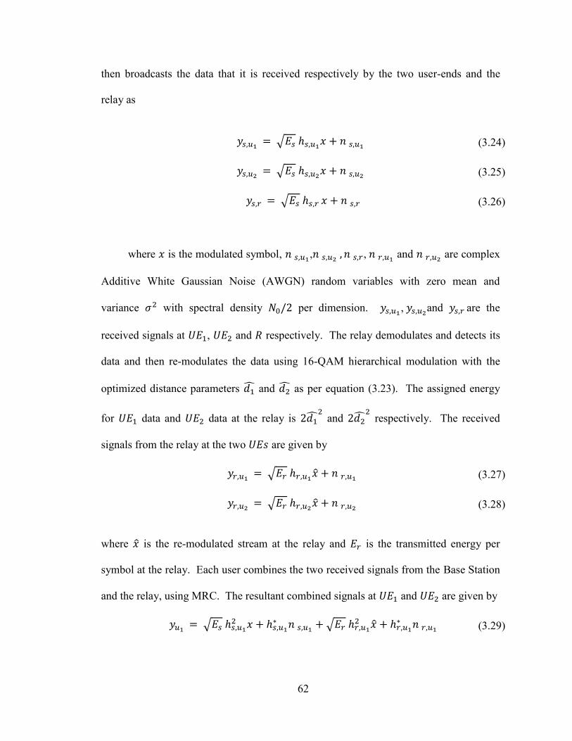
62
then broadcasts the data that it is received respectively by the two user-ends and the
relay as
√ ℎ
(3.24)
√ ℎ
(3.25)
√ ℎ (3.26)
where is the modulated symbol, ,
, and
are complex
Additive White Gaussian Noise (AWGN) random variables with zero mean and
variance with spectral density per dimension. ,
and are the
received signals at , and respectively. The relay demodulates and detects its
data and then re-modulates the data using 16-QAM hierarchical modulation with the
optimized distance parameters and as per equation (3.23). The assigned energy
for data and data at the relay is and
respectively. The received
signals from the relay at the two are given by
√ ℎ
(3.27)
√ ℎ
(3.28)
where is the re-modulated stream at the relay and is the transmitted energy per
symbol at the relay. Each user combines the two received signals from the Base Station
and the relay, using MRC. The resultant combined signals at and are given by
√ ℎ ℎ
√ ℎ
ℎ
(3.29)
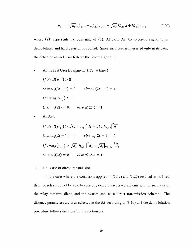
63
√ ℎ ℎ
√ ℎ
ℎ
(3.30)
where represents the conjugate of . At each , the received signal is
demodulated and hard decision is applied. Since each user is interested only in its data,
the detection at each user follows the below algorithm:
At the first User Equipment ( ) at time :
( )
ℎ
( )
ℎ
At :
( ) √ |ℎ | √ |ℎ
|
ℎ
( ) √ |ℎ | √ |ℎ
|
ℎ
3.3.2.1.2 Case of direct transmission
In the case where the conditions applied in (3.19) and (3.20) resulted in null set,
then the relay will not be able to correctly detect its received information. In such a case,
the relay remains silent, and the system acts as a direct transmission scheme. The
distance parameters are then selected at the according to (3.10) and the demodulation
procedure follows the algorithm in section 3.2.
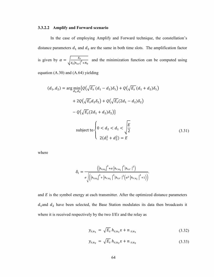
64
3.3.2.2 Amplify and Forward scenario
In the case of employing Amplify and Forward technique, the constellation’s
distance parameters and are the same in both time slots. The amplification factor
is given by √
| |
and the minimization function can be computed using
equation (A.30) and (A.64) yielding
{ (√ ) (√ )
(√ ) (√ )
(√ )}
{
√
(3.31)
where
(|
| |
| | |
)
√(| | |
| | |
( |
| ))
.
and is the symbol energy at each transmitter. After the optimized distance parameters
and have been selected, the Base Station modulates its data then broadcasts it
where it is received respectively by the two and the relay as
√ ℎ
(3.32)
√ ℎ
(3.33)
65
√ ℎ (3.34)
where is the modulated symbol and ,
and are complex Additive
White Gaussian Noise (AWGN) random variables with zero mean and variance
with spectral density per dimension. ,
and are the received signals
at , and the relay respectively. The relay simply amplifies the received signal
by an amplification gain √
| |
and resends it without any further
processing. The received signals from the relay at the User-Ends are given by
ℎ
for
ℎ
√ ℎ ℎ
(3.35)
and
are complex Additive White Gaussian Noise (AWGN) random
variables with zero mean and variance with spectral density per dimension.
At destination, each User-End combines the two received signals from the Base Station
and the Relay using MRC technique. The resultant combined signals at and
respectively are given by
√ |ℎ | ℎ
√ |ℎ |
|ℎ
|
|ℎ | ℎ ℎ
ℎ
(3.36)
and
66
√ |ℎ | ℎ
√ |ℎ |
|ℎ
|
|ℎ | ℎ ℎ
ℎ
(3.37)
The demodulation at each user follows the below algorithm:
At the first User Equipment ( ) at time :
( )
ℎ
( )
ℎ
At :
( ) ( |ℎ | |ℎ |
|ℎ
| ) √
ℎ
( ) ( |ℎ | |ℎ |
|ℎ
| ) √
ℎ
3.4 Turbo Coded Relay cooperation
In this section, the analysis is extended to the case of a Turbo coded cooperative
network. The system is composed of a , Relay and two User-Ends. The Base
Station concatenates and encodes the two streams of data. It modulates the resultant
stream then broadcasts it. They Relay receives the data along with the two User-Ends.
The data is demodulated and decoded at the Relay. A CRC takes place at the Relay. If
the CRC results in correct detection, the relay forwards the data using Decode and
67
Forward technique. The two User-Ends then combine the two signals by summing their
resultant LLRs from each path. If the CRC fails, then the Relay remains silent and the
destinations receive only one copy of the message from the .
3.4.1 Encoding Process
In this section, presentation of the structure of the Turbo encoder is illustrated.
Related parameters of the Turbo Encoder are given. The process of the Turbo encoding
including the input format, the interleaving, the puncturing and the channel interleaving
are presented in details in the following subsections.
3.4.1.1 Turbo Encoder Structure
The Turbo encoder used in the proposed system is shown in Figure 3.3. It
consists of two recursive systematic convolutional (RSC) encoders, each of constraint
length , concatenated in parallel. The feedforward generator is and the
feedback generator is . The number of input information bits to the Turbo
encoder is denoted by , . The two encoders are separated by an
interleaver where is an interleaved version of .
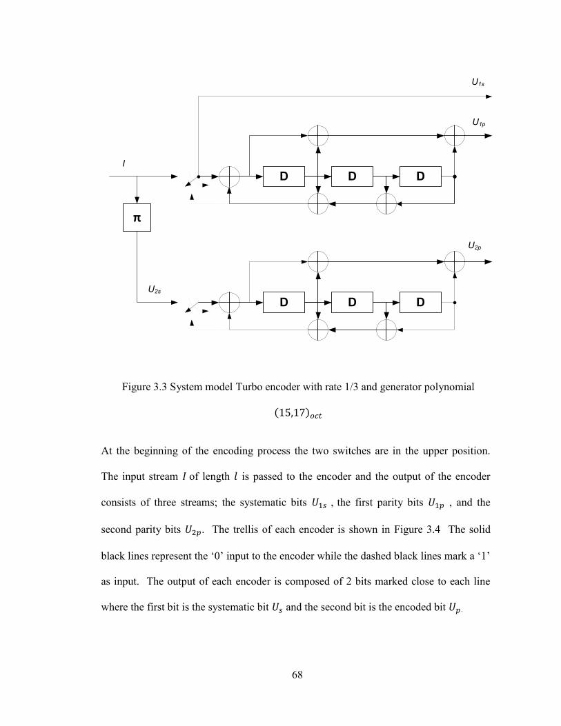
68
D D D
π
D D D
I
U2s
U1s
U1p
U2p
Figure 3.3 System model Turbo encoder with rate 1/3 and generator polynomial
At the beginning of the encoding process the two switches are in the upper position.
The input stream of length is passed to the encoder and the output of the encoder
consists of three streams; the systematic bits , the first parity bits , and the
second parity bits . The trellis of each encoder is shown in Figure 3.4 The solid
black lines represent the ‘0’ input to the encoder while the dashed black lines mark a ‘1’
as input. The output of each encoder is composed of 2 bits marked close to each line
where the first bit is the systematic bit and the second bit is the encoded bit .
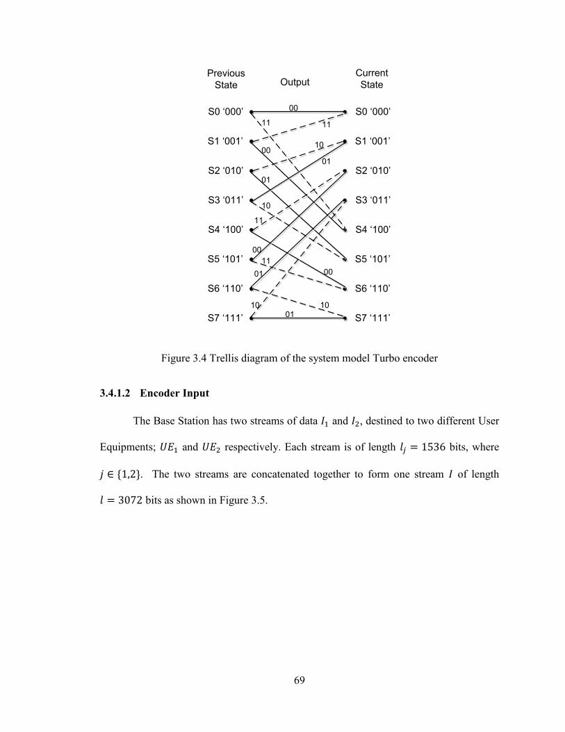
69
S0 ‘000’
S1 ‘001’
S2 ‘010’
S3 ‘011’
S4 ‘100’
S5 ‘101’
S6 ‘110’
S7 ‘111’
S0 ‘000’
S1 ‘001’
S2 ‘010’
S3 ‘011’
S4 ‘100’
S5 ‘101’
S6 ‘110’
S7 ‘111’
00
00
00
00
11 11
11
11
10
10
1010
01
01
01
01
Previous
State
Current
StateOutput
Figure 3.4 Trellis diagram of the system model Turbo encoder
3.4.1.2 Encoder Input
The Base Station has two streams of data and , destined to two different User
Equipments; and respectively. Each stream is of length bits, where
{ }. The two streams are concatenated together to form one stream of length
bits as shown in Figure 3.5.
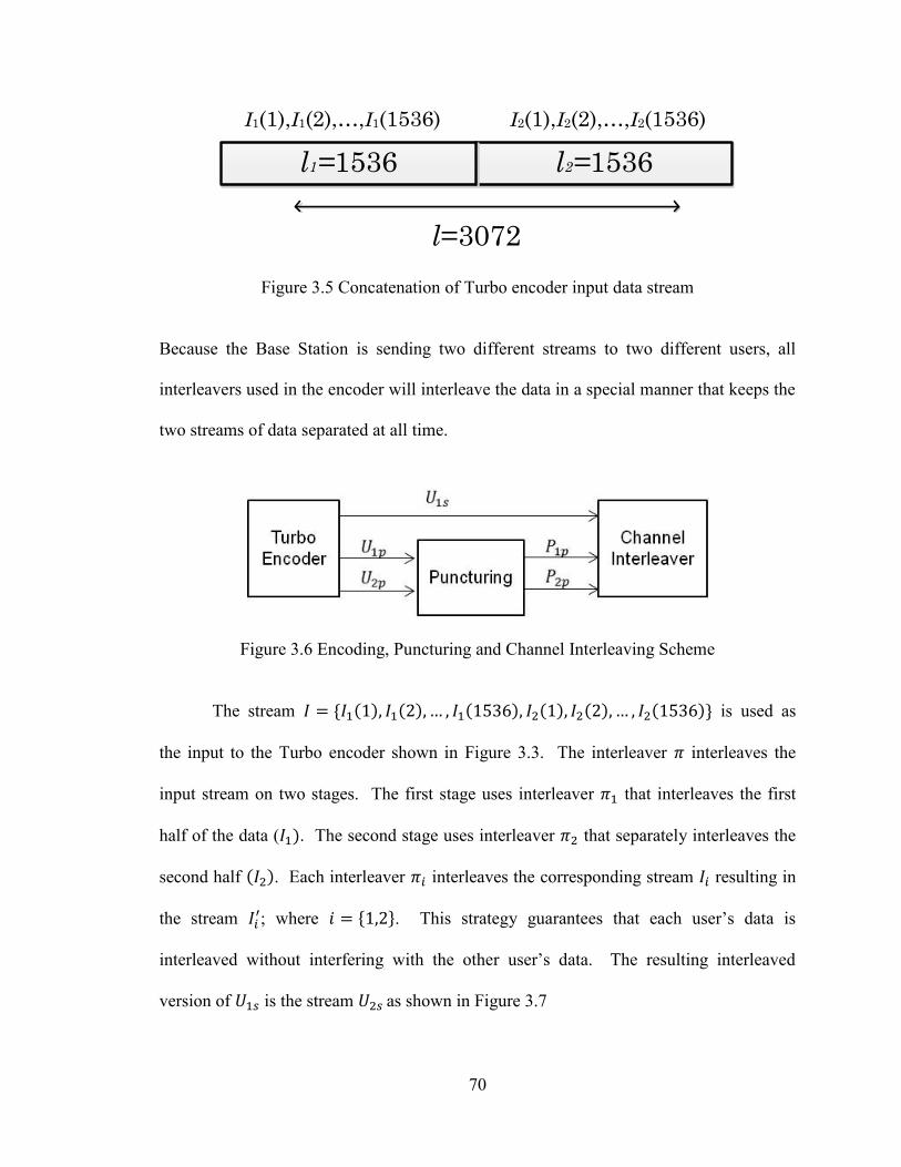
70
l1=1536 l2=1536
I1(1),I1(2),…,I1(1536) I2(1),I2(2),…,I2(1536)
l=3072
Figure 3.5 Concatenation of Turbo encoder input data stream
Because the Base Station is sending two different streams to two different users, all
interleavers used in the encoder will interleave the data in a special manner that keeps the
two streams of data separated at all time.
Figure 3.6 Encoding, Puncturing and Channel Interleaving Scheme
The stream { } is used as
the input to the Turbo encoder shown in Figure 3.3. The interleaver interleaves the
input stream on two stages. The first stage uses interleaver that interleaves the first
half of the data ( . The second stage uses interleaver that separately interleaves the
second half . Each interleaver interleaves the corresponding stream resulting in
the stream ; where { }. This strategy guarantees that each user’s data is
interleaved without interfering with the other user’s data. The resulting interleaved
version of is the stream as shown in Figure 3.7
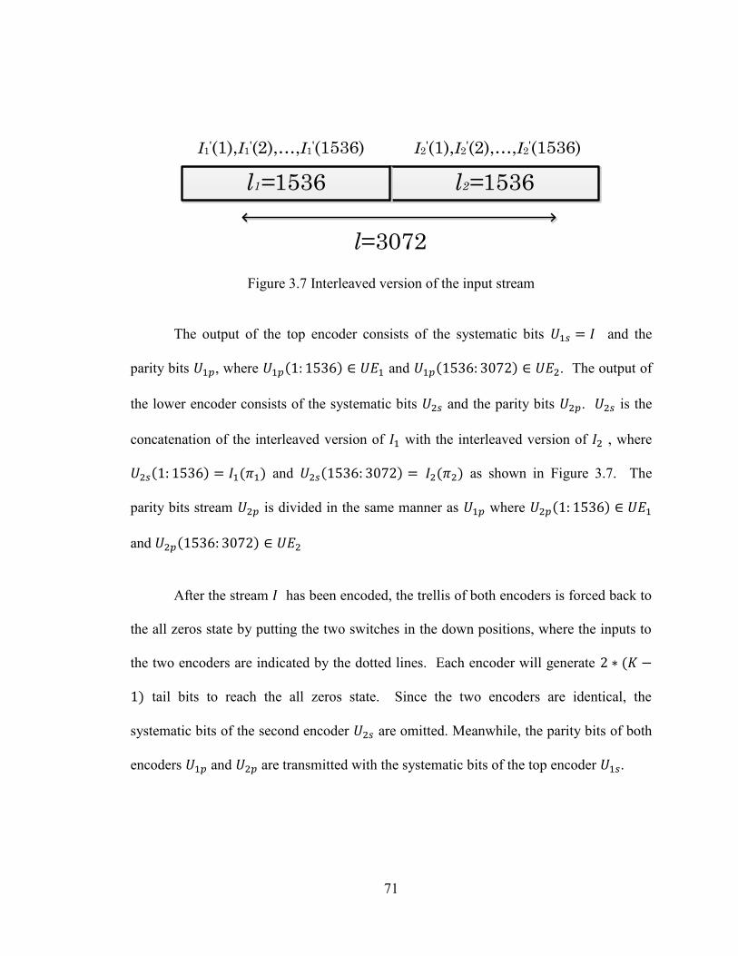
71
l1=1536 l2=1536
I1'(1),I1'(2),…,I1'(1536) I2'(1),I2'(2),…,I2'(1536)
l=3072
Figure 3.7 Interleaved version of the input stream
The output of the top encoder consists of the systematic bits and the
parity bits , where and . The output of
the lower encoder consists of the systematic bits and the parity bits . is the
concatenation of the interleaved version of with the interleaved version of , where
and as shown in Figure 3.7. The
parity bits stream is divided in the same manner as where
and
After the stream has been encoded, the trellis of both encoders is forced back to
the all zeros state by putting the two switches in the down positions, where the inputs to
the two encoders are indicated by the dotted lines. Each encoder will generate
tail bits to reach the all zeros state. Since the two encoders are identical, the
systematic bits of the second encoder are omitted. Meanwhile, the parity bits of both
encoders and are transmitted with the systematic bits of the top encoder .
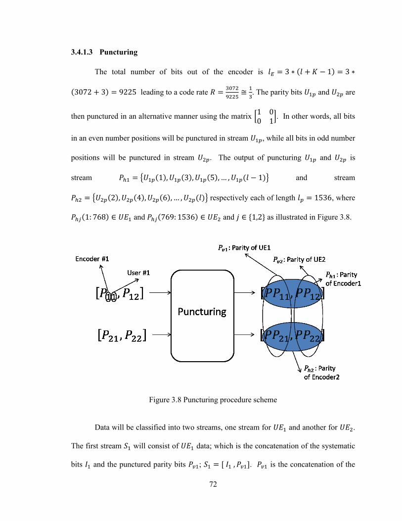
72
3.4.1.3 Puncturing
The total number of bits out of the encoder is
leading to a code rate
. The parity bits and are
then punctured in an alternative manner using the matrix [
]. In other words, all bits
in an even number positions will be punctured in stream , while all bits in odd number
positions will be punctured in stream . The output of puncturing and is
stream { } and stream
{ } respectively each of length , where
and and { } as illustrated in Figure 3.8.
Figure 3.8 Puncturing procedure scheme
Data will be classified into two streams, one stream for and another for .
The first stream will consist of data; which is the concatenation of the systematic
bits and the punctured parity bits ; [ ]. is the concatenation of the
73
parity bits of from the two encoders; [ ]; where
and . The second stream is the concatenation of data
consisting of the systematic bits and the punctured parity bits defined as ;
[ ]. is the concatenation of the parity bits of coming from the two
encoders; [ ], where and
.
3.4.1.4 Channel Interleaver
In order to simplify the input at the modulation process, inside each stream and
the systematic bits are interleaved independently from the parity bits. The systematic
bits of , , are interleaved using an interleaver of length
while the
parity bits of of , , are interleaved using an interleaver of the same length as
. The same applies for where bits are interleaved using and bits are
interleaved using . The result of the channel interleaving process is four separate
interleaved streams, each of length
. The first stream contains interleaved data
of the systematic bits of and is denoted by . The second stream is the interleaved
data of the parity bits of ; ; It is denoted by . The third stream is the
interleaved version of the systematic bits of and is denoted by . And the final
stream contains the interleaved parity bits of ; ; and is denoted by . The four
streams are then passed to the 16 QAM modulator.
The mapping at the input to the 16 QAM modulator consists of 4 streams, each
stream will be mapped to one of the 4 bits of the symbol. The first stream will be
mapped to the first bit . The second stream will be mapped to the second position
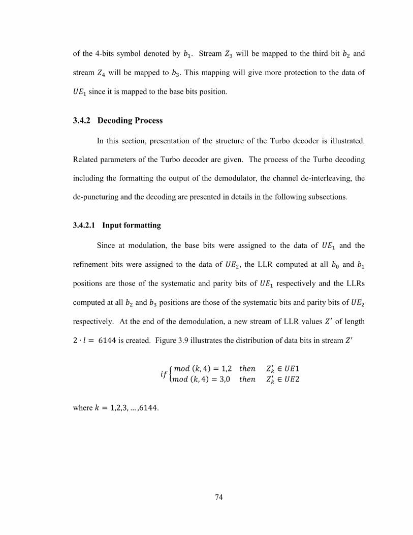
74
of the 4-bits symbol denoted by . Stream will be mapped to the third bit and
stream will be mapped to . This mapping will give more protection to the data of
since it is mapped to the base bits position.
3.4.2 Decoding Process
In this section, presentation of the structure of the Turbo decoder is illustrated.
Related parameters of the Turbo decoder are given. The process of the Turbo decoding
including the formatting the output of the demodulator, the channel de-interleaving, the
de-puncturing and the decoding are presented in details in the following subsections.
3.4.2.1 Input formatting
Since at modulation, the base bits were assigned to the data of and the
refinement bits were assigned to the data of , the LLR computed at all and
positions are those of the systematic and parity bits of respectively and the LLRs
computed at all and positions are those of the systematic bits and parity bits of
respectively. At the end of the demodulation, a new stream of LLR values of length
is created. Figure 3.9 illustrates the distribution of data bits in stream
{ ℎ
ℎ
where .
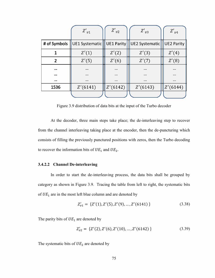
75
Figure 3.9 distribution of data bits at the input of the Turbo decoder
At the decoder, three main steps take place; the de-interleaving step to recover
from the channel interleaving taking place at the encoder, then the de-puncturing which
consists of filling the previously punctured positions with zeros, then the Turbo decoding
to recover the information bits of and .
3.4.2.2 Channel De-interleaving
In order to start the de-interleaving process, the data bits shall be grouped by
category as shown in Figure 3.9. Tracing the table from left to right, the systematic bits
of are in the most left blue column and are denoted by
{ } (3.38)
The parity bits of are denoted by
{ } (3.39)
The systematic bits of are denoted by
76
{ } (3.40)
And finally the parity bits of are denoted by
{ } (3.41)
After this grouping, each group is de-interleaved using the corresponding inverse of the
interleaver function used at the encoder. The four resulting streams out of the de-
interleaving process are denoted as follow
(3.42)
(3.43)
and
(3.44)
(3.45)
From the two streams and
we recover the two streams and
as illustrated in
Figure 3.8 where
[
] (3.46)
and
[
] (3.47)
3.4.2.3 De-puncturing
The de-puncturing process takes place in the parity bits of the first encoder, ,
and the parity bits of the second encoder, . It consists of inserting zeros in the
previously punctured positions. In other words, a zero is inserted ‘after’ every bit of the
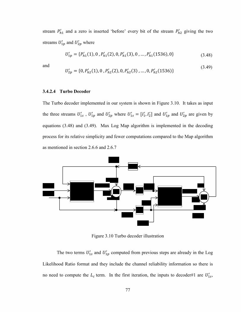
77
stream and a zero is inserted ‘before’ every bit of the stream
giving the two
streams and
where
{
} (3.48)
and
{
}
(3.49)
3.4.2.4 Turbo Decoder
The Turbo decoder implemented in our system is shown in Figure 3.10. It takes as input
the three streams ,
and where
[
] and and
are given by
equations (3.48) and (3.49). Max Log Map algorithm is implemented in the decoding
process for its relative simplicity and fewer computations compared to the Map algorithm
as mentioned in section 2.6.6 and 2.6.7
Figure 3.10 Turbo decoder illustration
The two terms and
computed from previous steps are already in the Log
Likelihood Ratio format and they include the channel reliability information so there is
no need to compute the term. In the first iteration, the inputs to decoder#1 are ,
Decoder
#1
Decoder
#2
∑
∑
π
π
78
and
where . is set to zero at the beginning of the decoding
process as equal probability for the input binary bits is assumed.
The group of equations (2.9) to (2.12) are solved at this stage in an iterative
manner as shown in Figure 3.10 using Max Log MAP algorithm to obtain an accurate
estimate of the a posteriori probability (APP) of the information bits. In the presented
system, four iterations are employed. At the end of the iterative process a hard decision
is made according to
{
(3.50)
where is the de-interleaved version of
3.5 Summary
In this chapter, the proposed system model for this thesis was reviewed. Different
schemes for the proposed system including direct transmission, user cooperation, relay
node cooperation and finally Turbo coded relay cooperation were presented. Different
system parameters related to the modulation/demodulation and encoding/decoding
processes were given. In the next chapter, results of all the above mentioned systems will
be presented comparing the performance of the traditional uniform constellation with the
proposed one.
79
Chapter Four
Results and Discussion 4.
In this chapter, a discussion on the related simulation results is presented.
Simulations of direct transmission, user cooperation, relay cooperation and Turbo codes
relay cooperation system models are examined. In each of the mentioned systems,
comparison between the different users BER in a uniform modulation based system and
an optimized hierarchical modulation based system are illustrated. In each of these
comparisons, it is proven that the optimized hierarchical modulation improves the
performance of both users compared to the uniform modulation.
4.1 Direct Transmission
Although the main focus of this thesis is the study of hierarchical modulation in
cooperative networks, the study of hierarchical modulation in direct transmission is
mandatory. Its importance lies in the fact that it clearly illustrates how the variation in
80
the distance parameters of a 4/16 QAM constellation can change the performance of both
the base and the refinement bits. In this section, it is proven by simulations that
optimized selection of the constellation’s parameters in fact does improve both the base
bits stream and the refinement bits stream BER. As mentioned in Section 3.2, the scheme
of the direct transmission consists of a Base Station ( ) sending two different streams of
data simultaneously to two different users by employing a hierarchical 16 QAM
modulation. The data of is mapped to the base bits while the data of is mapped
to the refinement bits. Simulations in the case of Direct Transmission compare three
different inter-nodes distances to examine the effect of the relative physical distances of
the nodes on the performance. In order to show such effect, the results are plotted in
terms of transmitted SNR, and this transmitted SNR is defined as
⁄ , and
is the transmitted symbol energy at the . In the following simulation results, the
distance between the and is denoted by for { }.
4.1.1 Case (
)
This case studies the scenario where both User-Ends are at the same physical
distance from the . For simplicity we assume
, where the path loss
exponent is assumed to have a value of 3.5. Comparison between the BER
performance of the base bits and the refinement bits using a uniform 16QAM using an
optimized hierarchical 16QAM is illustrated in Figure 4.1 and Figure 4.2. In Figure 4.1,
the base bits BER using an optimized constellation has a higher performance of 2-4 dB
compared to uniform constellation. Meanwhile, Figure 4.2 illustrates the case of
refinement bits BER. It is shown in the Figure that the performance using the optimized
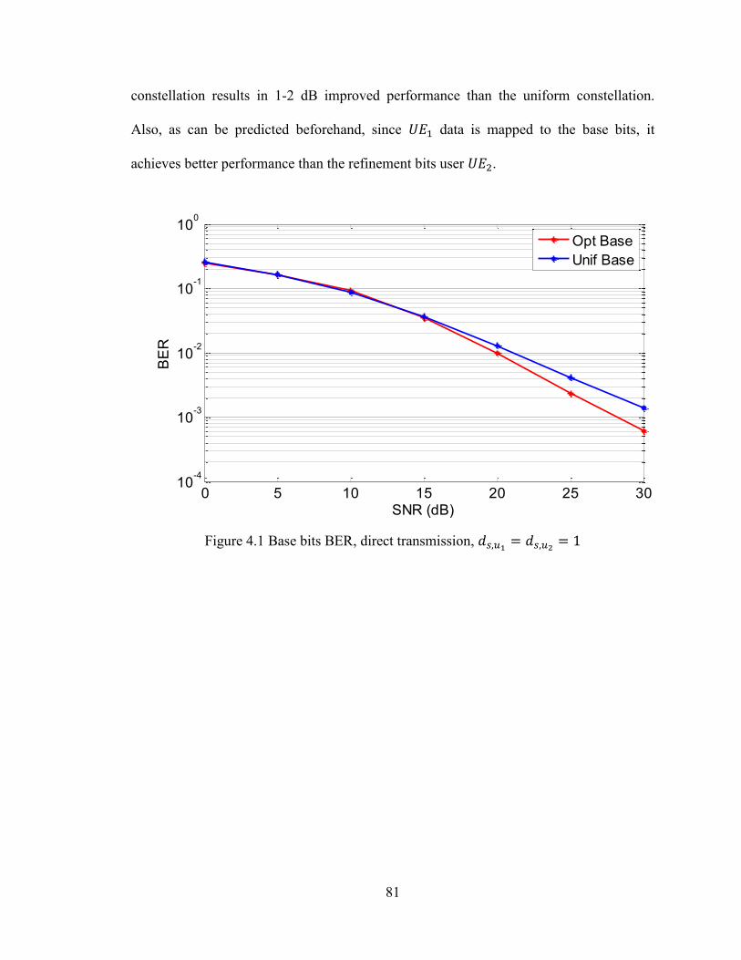
81
constellation results in 1-2 dB improved performance than the uniform constellation.
Also, as can be predicted beforehand, since data is mapped to the base bits, it
achieves better performance than the refinement bits user .
Figure 4.1 Base bits BER, direct transmission,
0 5 10 15 20 25 3010
-4
10-3
10-2
10-1
100
SNR (dB)
BE
R
Opt Base
Unif Base
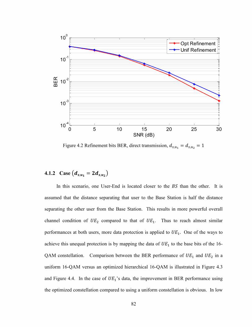
82
Figure 4.2 Refinement bits BER, direct transmission,
4.1.2 Case (
)
In this scenario, one User-End is located closer to the than the other. It is
assumed that the distance separating that user to the Base Station is half the distance
separating the other user from the Base Station. This results in more powerful overall
channel condition of compared to that of . Thus to reach almost similar
performances at both users, more data protection is applied to One of the ways to
achieve this unequal protection is by mapping the data of to the base bits of the 16-
QAM constellation. Comparison between the BER performance of and in a
uniform 16-QAM versus an optimized hierarchical 16-QAM is illustrated in Figure 4.3
and Figure 4.4. In the case of ’s data, the improvement in BER performance using
the optimized constellation compared to using a uniform constellation is obvious. In low
0 5 10 15 20 25 3010
-4
10-3
10-2
10-1
100
SNR (dB)
BE
R
Opt Refinement
Unif Refinement
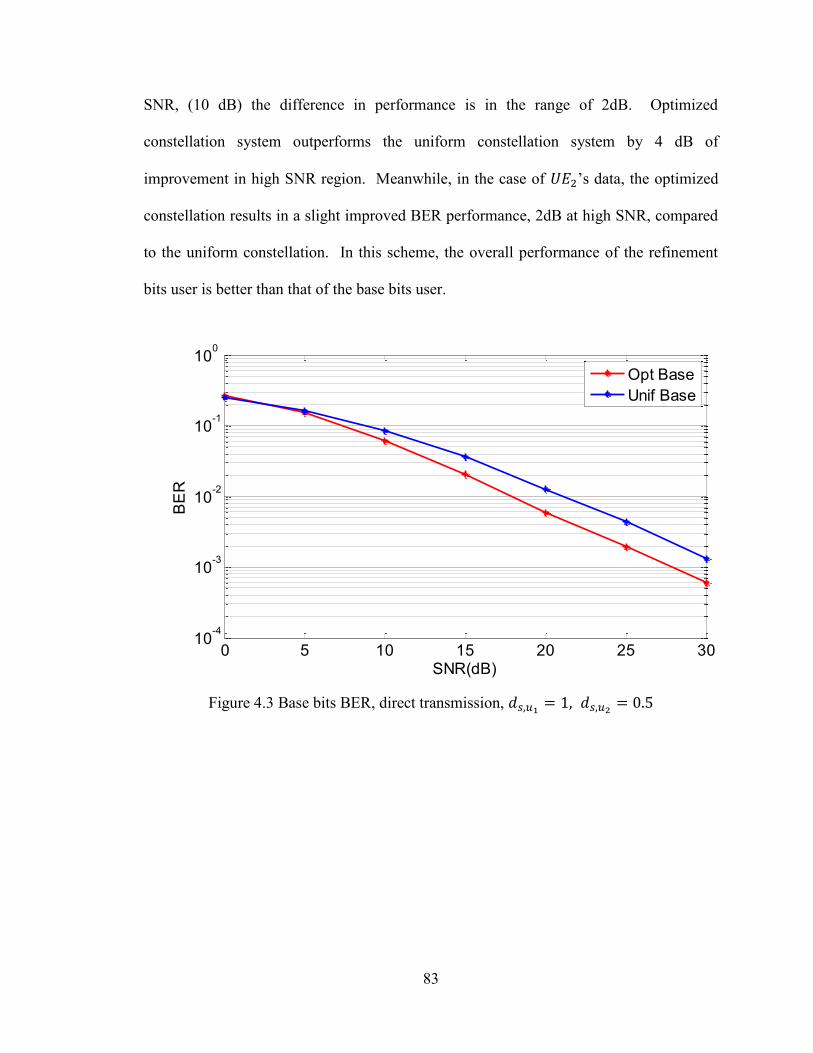
83
SNR, (10 dB) the difference in performance is in the range of 2dB. Optimized
constellation system outperforms the uniform constellation system by 4 dB of
improvement in high SNR region. Meanwhile, in the case of ’s data, the optimized
constellation results in a slight improved BER performance, 2dB at high SNR, compared
to the uniform constellation. In this scheme, the overall performance of the refinement
bits user is better than that of the base bits user.
Figure 4.3 Base bits BER, direct transmission,
0 5 10 15 20 25 3010
-4
10-3
10-2
10-1
100
SNR(dB)
BE
R
Opt Base
Unif Base
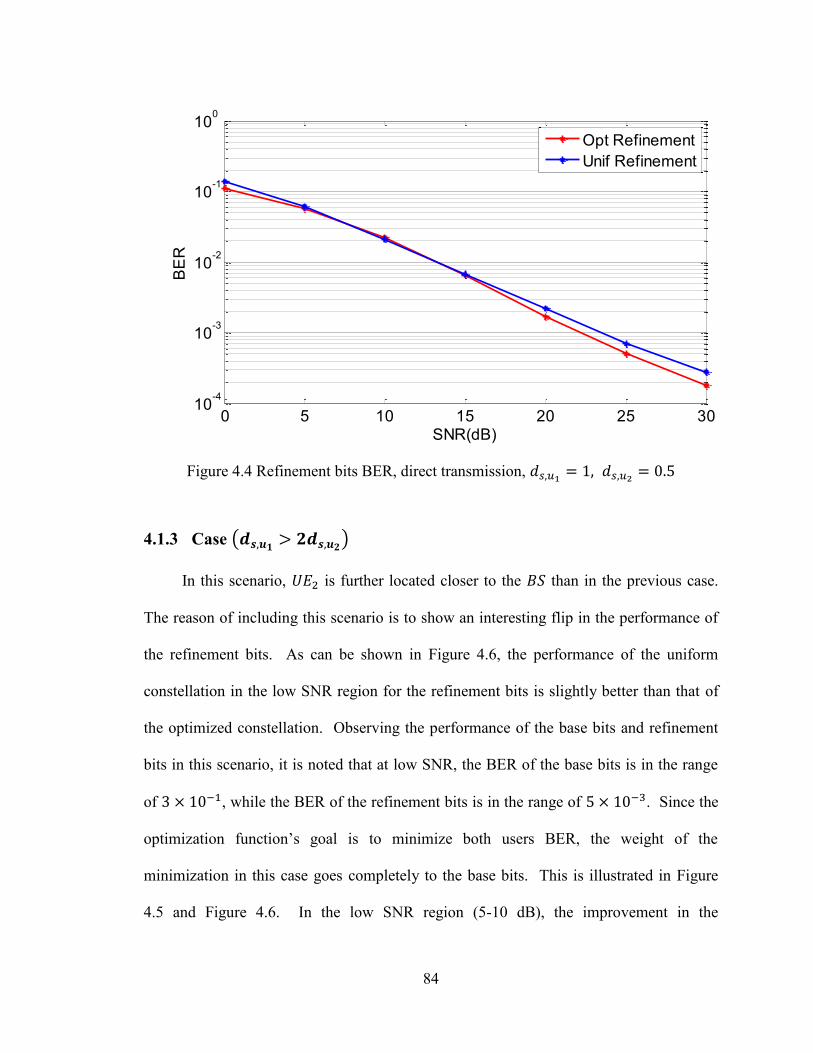
84
Figure 4.4 Refinement bits BER, direct transmission,
4.1.3 Case (
)
In this scenario, is further located closer to the than in the previous case.
The reason of including this scenario is to show an interesting flip in the performance of
the refinement bits. As can be shown in Figure 4.6, the performance of the uniform
constellation in the low SNR region for the refinement bits is slightly better than that of
the optimized constellation. Observing the performance of the base bits and refinement
bits in this scenario, it is noted that at low SNR, the BER of the base bits is in the range
of , while the BER of the refinement bits is in the range of . Since the
optimization function’s goal is to minimize both users BER, the weight of the
minimization in this case goes completely to the base bits. This is illustrated in Figure
4.5 and Figure 4.6. In the low SNR region (5-10 dB), the improvement in the
0 5 10 15 20 25 3010
-4
10-3
10-2
10-1
100
SNR(dB)
BE
R
Opt Refinement
Unif Refinement
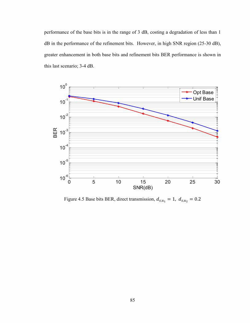
85
performance of the base bits is in the range of 3 dB, costing a degradation of less than 1
dB in the performance of the refinement bits. However, in high SNR region (25-30 dB),
greater enhancement in both base bits and refinement bits BER performance is shown in
this last scenario; 3-4 dB.
Figure 4.5 Base bits BER, direct transmission,
0 5 10 15 20 25 3010
-6
10-5
10-4
10-3
10-2
10-1
100
SNR(dB)
BE
R
Opt Base
Unif Base
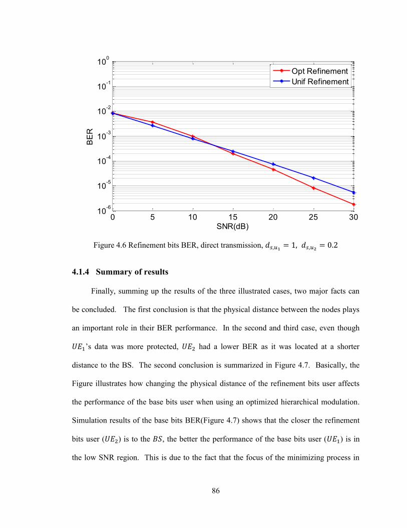
86
Figure 4.6 Refinement bits BER, direct transmission,
4.1.4 Summary of results
Finally, summing up the results of the three illustrated cases, two major facts can
be concluded. The first conclusion is that the physical distance between the nodes plays
an important role in their BER performance. In the second and third case, even though
’s data was more protected, had a lower BER as it was located at a shorter
distance to the BS. The second conclusion is summarized in Figure 4.7. Basically, the
Figure illustrates how changing the physical distance of the refinement bits user affects
the performance of the base bits user when using an optimized hierarchical modulation.
Simulation results of the base bits BER(Figure 4.7) shows that the closer the refinement
bits user ( ) is to the , the better the performance of the base bits user ( ) is in
the low SNR region. This is due to the fact that the focus of the minimizing process in
0 5 10 15 20 25 3010
-6
10-5
10-4
10-3
10-2
10-1
100
SNR(dB)
BE
R
Opt Refinement
Unif Refinement
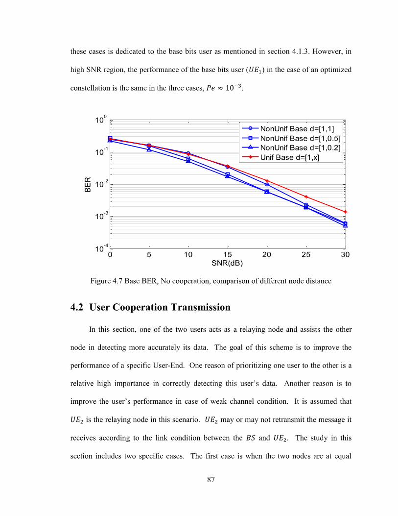
87
these cases is dedicated to the base bits user as mentioned in section 4.1.3. However, in
high SNR region, the performance of the base bits user ( ) in the case of an optimized
constellation is the same in the three cases, .
Figure 4.7 Base BER, No cooperation, comparison of different node distance
4.2 User Cooperation Transmission
In this section, one of the two users acts as a relaying node and assists the other
node in detecting more accurately its data. The goal of this scheme is to improve the
performance of a specific User-End. One reason of prioritizing one user to the other is a
relative high importance in correctly detecting this user’s data. Another reason is to
improve the user’s performance in case of weak channel condition. It is assumed that
is the relaying node in this scenario. may or may not retransmit the message it
receives according to the link condition between the and . The study in this
section includes two specific cases. The first case is when the two nodes are at equal
0 5 10 15 20 25 3010
-4
10-3
10-2
10-1
100
SNR(dB)
BE
R
NonUnif Base d=[1,1]
NonUnif Base d=[1,0.5]
NonUnif Base d=[1,0.2]
Unif Base d=[1,x]
88
separating distance from the . The second case is when one node; , is closer to
than , specifically when
. In the User Cooperation transmission
scheme, both; the 16-QAM constellation’s parameters and the total transmitted energy;
are optimized in order to achieve minimum total BER. The 16-QAM constellation’s
parameters control the distribution of the available transmitted energy on the two users at
the transmitting node. The optimization of the total transmitted energy is the distribution
of energy on the BS and the assisting node in order to achieve minimum BER. Since the
goal of this transmission model is to improve the performance of only one user, only the
performance of that user (base bits user) is presented in this section. Comparison
between the BER performance of in user cooperation transmission and in direct
transmission is examined.
4.2.1 Case (
)
In this case, the correct reception of data is of relative high importance that
that of . It is assumed that both User-Ends are at the same physical distance from the
, specifically
. The path loss exponent is assumed to have a value
of 3.5. The performance of is illustrated in Figure 4.8. A comparison between
’s BER when employing a uniform 16QAM modulation and when employing an
optimized hierarchical 16QAM modulation is presented. Also a comparison between
performance of the Direct Transmission case and the case of user cooperation is
illustrated. Results show that the performance of the base bits in the user cooperation
model is superior to that of the direct transmission model by 2.5 dB. Meanwhile,
optimization of both the transmitted power and the constellation’s distance parameters at
the improves the performance by 2 dB.
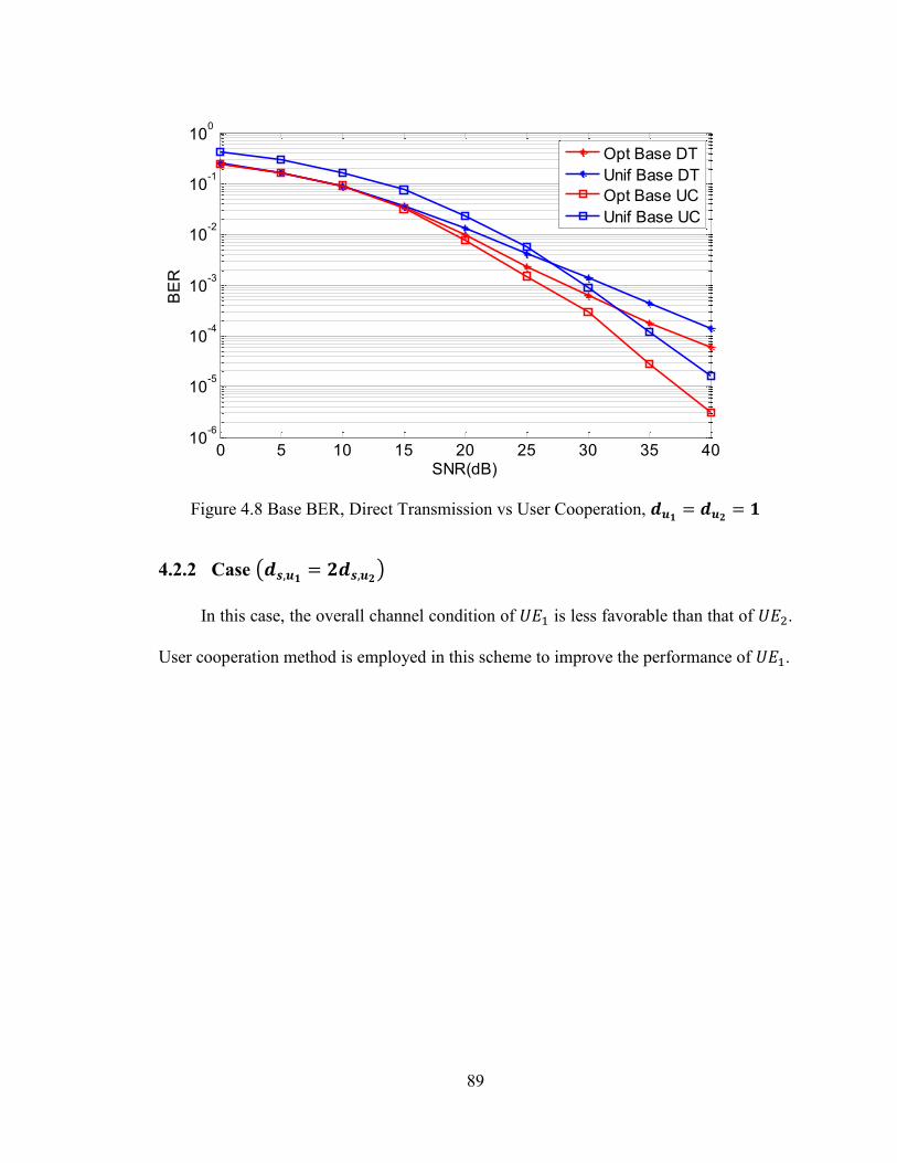
89
Figure 4.8 Base BER, Direct Transmission vs User Cooperation,
4.2.2 Case (
)
In this case, the overall channel condition of is less favorable than that of .
User cooperation method is employed in this scheme to improve the performance of .
0 5 10 15 20 25 30 35 4010
-6
10-5
10-4
10-3
10-2
10-1
100
SNR(dB)
BE
R
Opt Base DT
Unif Base DT
Opt Base UC
Unif Base UC
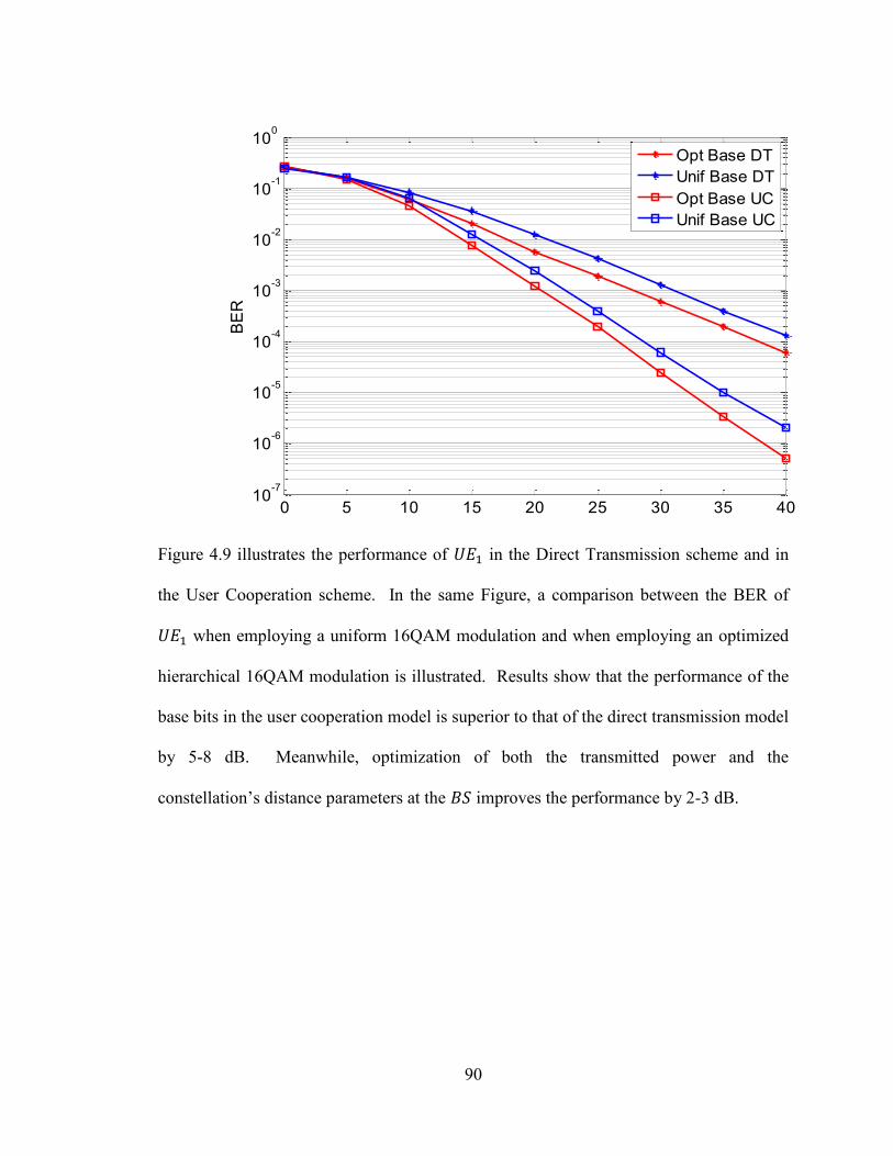
90
Figure 4.9 illustrates the performance of in the Direct Transmission scheme and in
the User Cooperation scheme. In the same Figure, a comparison between the BER of
when employing a uniform 16QAM modulation and when employing an optimized
hierarchical 16QAM modulation is illustrated. Results show that the performance of the
base bits in the user cooperation model is superior to that of the direct transmission model
by 5-8 dB. Meanwhile, optimization of both the transmitted power and the
constellation’s distance parameters at the improves the performance by 2-3 dB.
0 5 10 15 20 25 30 35 4010
-7
10-6
10-5
10-4
10-3
10-2
10-1
100
SNR(dB)
BE
R
Opt Base DT
Unif Base DT
Opt Base UC
Unif Base UC
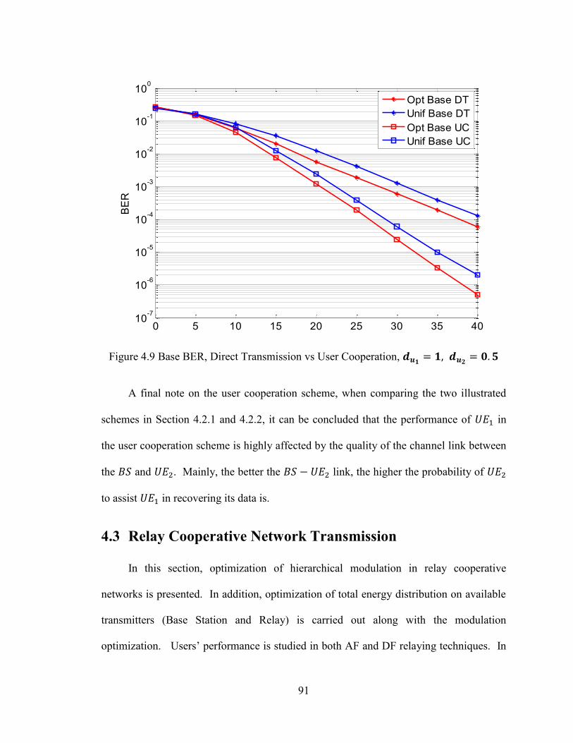
91
Figure 4.9 Base BER, Direct Transmission vs User Cooperation,
A final note on the user cooperation scheme, when comparing the two illustrated
schemes in Section 4.2.1 and 4.2.2, it can be concluded that the performance of in
the user cooperation scheme is highly affected by the quality of the channel link between
the and . Mainly, the better the link, the higher the probability of
to assist in recovering its data is.
4.3 Relay Cooperative Network Transmission
In this section, optimization of hierarchical modulation in relay cooperative
networks is presented. In addition, optimization of total energy distribution on available
transmitters (Base Station and Relay) is carried out along with the modulation
optimization. Users’ performance is studied in both AF and DF relaying techniques. In
0 5 10 15 20 25 30 35 4010
-7
10-6
10-5
10-4
10-3
10-2
10-1
100
SNR(dB)
BE
R
Opt Base DT
Unif Base DT
Opt Base UC
Unif Base UC
92
the following subsections, a study on the effect of changing the relay node location on the
performance of the users BER is presented. Later, another study on the effect of changing
one destination node location on the BER of both destinations is presented. In each of
the presented scenarios, three modulation and energy distribution techniques are
examined. The first case employs a uniform constellation with equal energy distribution
at the and the Relay. The second case employs an optimized hierarchical modulation
at both the and the Relay while still keeping equal energy distribution at both
transmitters. The second case will be referred to as Modulation Optimization (MO). The
third case employs an optimized modulation at both the and the Relay while
optimizing the transmitted energy at these two nodes. The third case will be referred to
as Modulation and Power Optimization (MPO). Results in this section are plotted in
terms of transmitted SNR, where the transmitted SNR is defined by ⁄
⁄ , where is the transmitted energy at the source and is the transmitted energy
at the relay.
4.3.1 Effect of changing the location of the Relay node
In this subsection, analysis of the effect of the relative relay node location to the
Base Station is carried out for both AF and DF relaying techniques. This analysis is
conducted for both base bits user and refinement bits user . Three cases of relay
node location are examined; the relay is closer to the , the relay is half way between
the and the , the relay is closer to the .
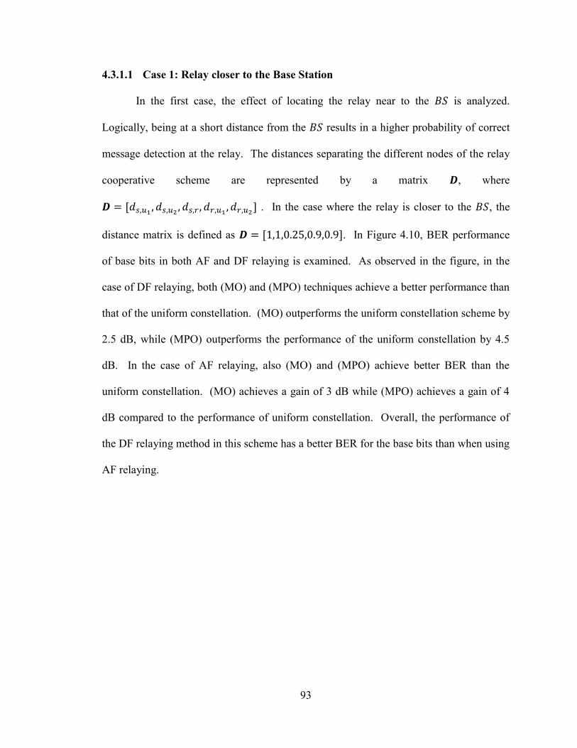
93
4.3.1.1 Case 1: Relay closer to the Base Station
In the first case, the effect of locating the relay near to the is analyzed.
Logically, being at a short distance from the results in a higher probability of correct
message detection at the relay. The distances separating the different nodes of the relay
cooperative scheme are represented by a matrix , where
[
] . In the case where the relay is closer to the , the
distance matrix is defined as [ ]. In Figure 4.10, BER performance
of base bits in both AF and DF relaying is examined. As observed in the figure, in the
case of DF relaying, both (MO) and (MPO) techniques achieve a better performance than
that of the uniform constellation. (MO) outperforms the uniform constellation scheme by
2.5 dB, while (MPO) outperforms the performance of the uniform constellation by 4.5
dB. In the case of AF relaying, also (MO) and (MPO) achieve better BER than the
uniform constellation. (MO) achieves a gain of 3 dB while (MPO) achieves a gain of 4
dB compared to the performance of uniform constellation. Overall, the performance of
the DF relaying method in this scheme has a better BER for the base bits than when using
AF relaying.
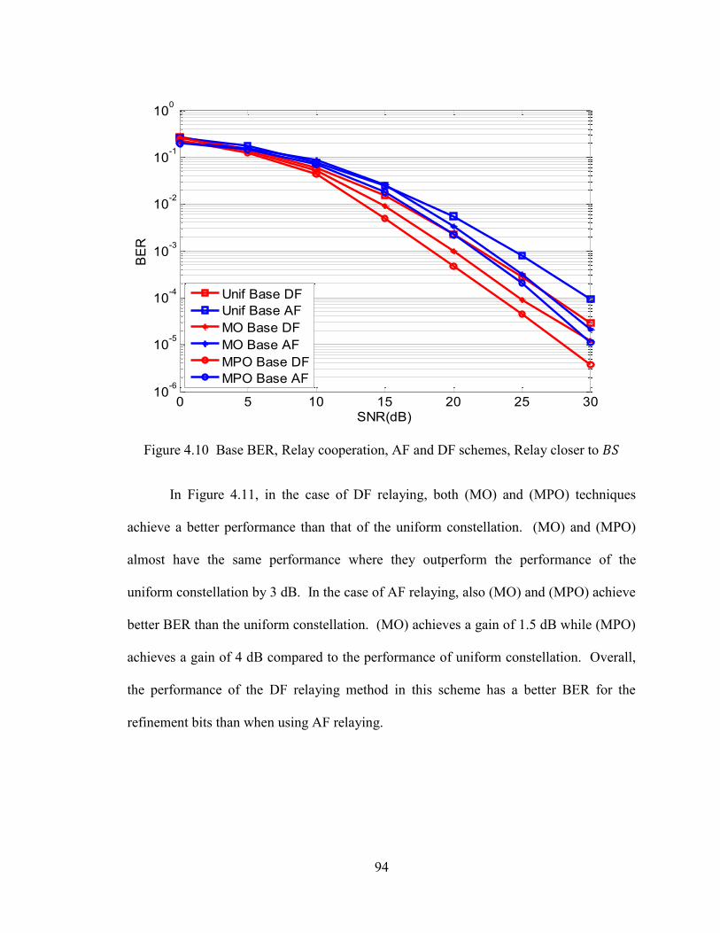
94
Figure 4.10 Base BER, Relay cooperation, AF and DF schemes, Relay closer to
In Figure 4.11, in the case of DF relaying, both (MO) and (MPO) techniques
achieve a better performance than that of the uniform constellation. (MO) and (MPO)
almost have the same performance where they outperform the performance of the
uniform constellation by 3 dB. In the case of AF relaying, also (MO) and (MPO) achieve
better BER than the uniform constellation. (MO) achieves a gain of 1.5 dB while (MPO)
achieves a gain of 4 dB compared to the performance of uniform constellation. Overall,
the performance of the DF relaying method in this scheme has a better BER for the
refinement bits than when using AF relaying.
0 5 10 15 20 25 3010
-6
10-5
10-4
10-3
10-2
10-1
100
SNR(dB)
BE
R
Unif Base DF
Unif Base AF
MO Base DF
MO Base AF
MPO Base DF
MPO Base AF
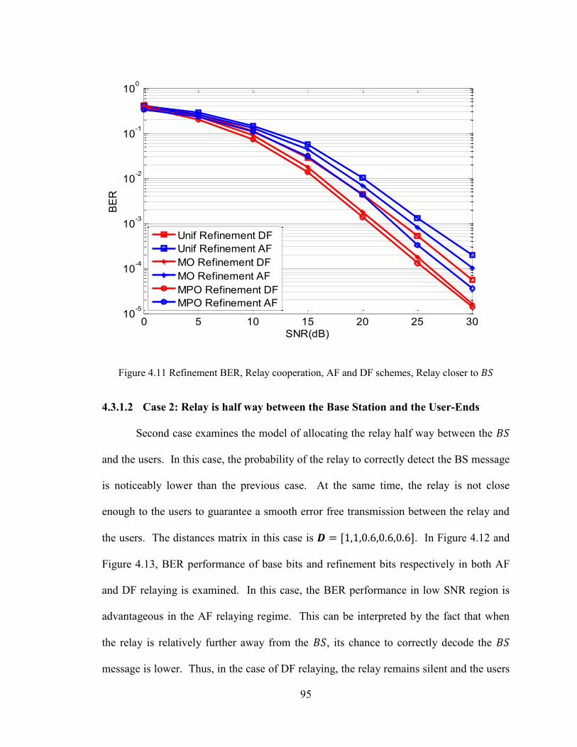
95
Figure 4.11 Refinement BER, Relay cooperation, AF and DF schemes, Relay closer to
4.3.1.2 Case 2: Relay is half way between the Base Station and the User-Ends
Second case examines the model of allocating the relay half way between the
and the users. In this case, the probability of the relay to correctly detect the BS message
is noticeably lower than the previous case. At the same time, the relay is not close
enough to the users to guarantee a smooth error free transmission between the relay and
the users. The distances matrix in this case is [ ]. In Figure 4.12 and
Figure 4.13, BER performance of base bits and refinement bits respectively in both AF
and DF relaying is examined. In this case, the BER performance in low SNR region is
advantageous in the AF relaying regime. This can be interpreted by the fact that when
the relay is relatively further away from the , its chance to correctly decode the
message is lower. Thus, in the case of DF relaying, the relay remains silent and the users
0 5 10 15 20 25 3010
-5
10-4
10-3
10-2
10-1
100
SNR(dB)
BE
R
Unif Refinement DF
Unif Refinement AF
MO Refinement DF
MO Refinement AF
MPO Refinement DF
MPO Refinement AF
96
receives only one copy of the message. However, in the case of AF relaying, where the
relay forwards its received message anyway, the probability of achieving diversity is
higher. Meanwhile, at high SNR region, when the relay can reliably detect the BS
message, DF’s performance is superior to AF. Logically, this is because at the user side,
the probability of correctly detecting a clean message (DF) is higher than detecting a
noisy message (AF).
In Figure 4.12, in the low SNR region (0-10 dB) in DF relaying, the (MO) scheme
has the same performance as that of uniform modulation, while the performance of the
(MPO) scheme is superior to both of them by an average of 2dB. The performances of
(MO) and (MPO) improve at high SNR to outperform the uniform modulation model by
2.5 dB and 5dB respectively. In AF relaying, (MO) has a 1dB gain compared to uniform
modulation scenario, while (MPO) outperforms them both in high SNR region (20-30
dB) to reach an average value of 6dB.
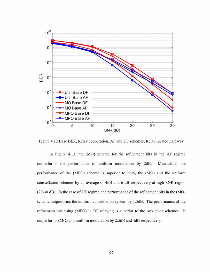
97
Figure 4.12 Base BER, Relay cooperation, AF and DF schemes, Relay located half way
In Figure 4.13, the (MO) scheme for the refinement bits in the AF regime
outperforms the performance of uniform modulation by 2dB. Meanwhile, the
performance of the (MPO) scheme is superior to both, the (MO) and the uniform
constellation schemes by an average of 4dB and 6 dB respectively at high SNR region
(20-30 dB). In the case of DF regime, the performance of the refinement bits in the (MO)
scheme outperforms the uniform constellation system by 1.5dB. The performance of the
refinement bits using (MPO) in DF relaying is superior to the two other schemes. It
outperforms (MO) and uniform modulation by 2.5dB and 4dB respectively.
0 5 10 15 20 25 3010
-6
10-5
10-4
10-3
10-2
10-1
100
SNR(dB)
BE
R
Unif Base DF
Unif Base AF
MO Base DF
MO Base AF
MPO Base DF
MPO Base AF
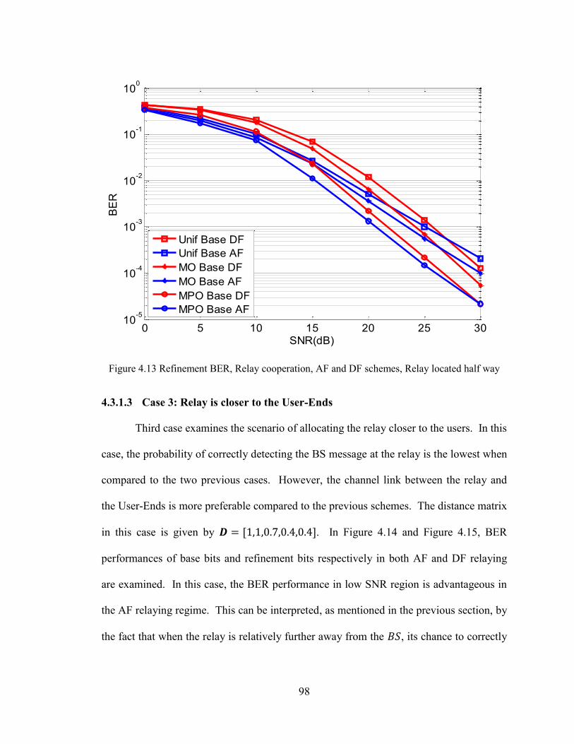
98
Figure 4.13 Refinement BER, Relay cooperation, AF and DF schemes, Relay located half way
4.3.1.3 Case 3: Relay is closer to the User-Ends
Third case examines the scenario of allocating the relay closer to the users. In this
case, the probability of correctly detecting the BS message at the relay is the lowest when
compared to the two previous cases. However, the channel link between the relay and
the User-Ends is more preferable compared to the previous schemes. The distance matrix
in this case is given by [ ]. In Figure 4.14 and Figure 4.15, BER
performances of base bits and refinement bits respectively in both AF and DF relaying
are examined. In this case, the BER performance in low SNR region is advantageous in
the AF relaying regime. This can be interpreted, as mentioned in the previous section, by
the fact that when the relay is relatively further away from the , its chance to correctly
0 5 10 15 20 25 3010
-5
10-4
10-3
10-2
10-1
100
SNR(dB)
BE
R
Unif Base DF
Unif Base AF
MO Base DF
MO Base AF
MPO Base DF
MPO Base AF
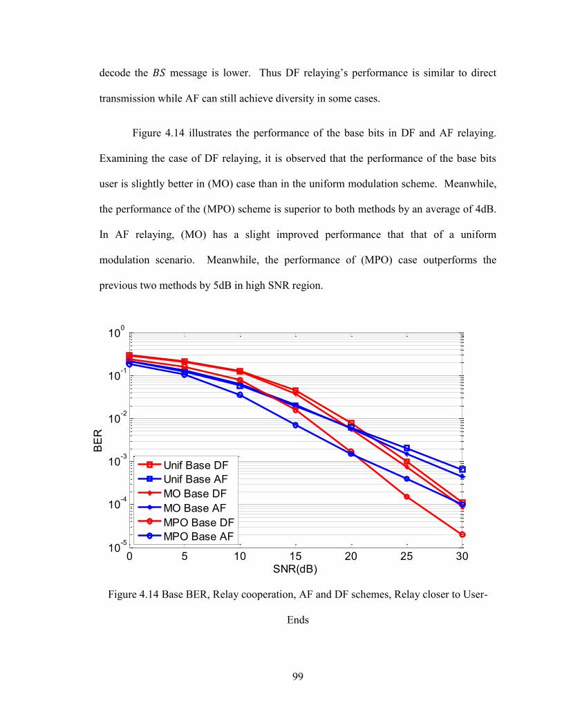
99
decode the message is lower. Thus DF relaying’s performance is similar to direct
transmission while AF can still achieve diversity in some cases.
Figure 4.14 illustrates the performance of the base bits in DF and AF relaying.
Examining the case of DF relaying, it is observed that the performance of the base bits
user is slightly better in (MO) case than in the uniform modulation scheme. Meanwhile,
the performance of the (MPO) scheme is superior to both methods by an average of 4dB.
In AF relaying, (MO) has a slight improved performance that that of a uniform
modulation scenario. Meanwhile, the performance of (MPO) case outperforms the
previous two methods by 5dB in high SNR region.
Figure 4.14 Base BER, Relay cooperation, AF and DF schemes, Relay closer to User-
Ends
0 5 10 15 20 25 3010
-5
10-4
10-3
10-2
10-1
100
SNR(dB)
BE
R
Unif Base DF
Unif Base AF
MO Base DF
MO Base AF
MPO Base DF
MPO Base AF
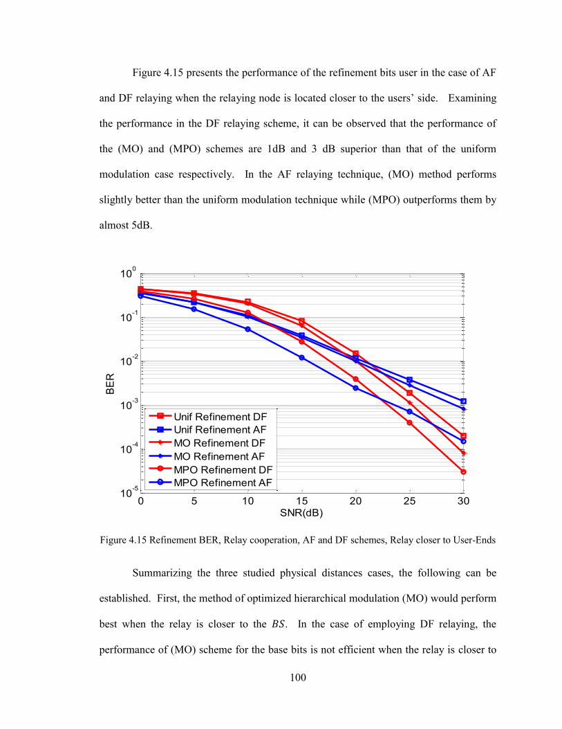
100
Figure 4.15 presents the performance of the refinement bits user in the case of AF
and DF relaying when the relaying node is located closer to the users’ side. Examining
the performance in the DF relaying scheme, it can be observed that the performance of
the (MO) and (MPO) schemes are 1dB and 3 dB superior than that of the uniform
modulation case respectively. In the AF relaying technique, (MO) method performs
slightly better than the uniform modulation technique while (MPO) outperforms them by
almost 5dB.
Figure 4.15 Refinement BER, Relay cooperation, AF and DF schemes, Relay closer to User-Ends
Summarizing the three studied physical distances cases, the following can be
established. First, the method of optimized hierarchical modulation (MO) would perform
best when the relay is closer to the . In the case of employing DF relaying, the
performance of (MO) scheme for the base bits is not efficient when the relay is closer to
0 5 10 15 20 25 3010
-5
10-4
10-3
10-2
10-1
100
SNR(dB)
BE
R
Unif Refinement DF
Unif Refinement AF
MO Refinement DF
MO Refinement AF
MPO Refinement DF
MPO Refinement AF
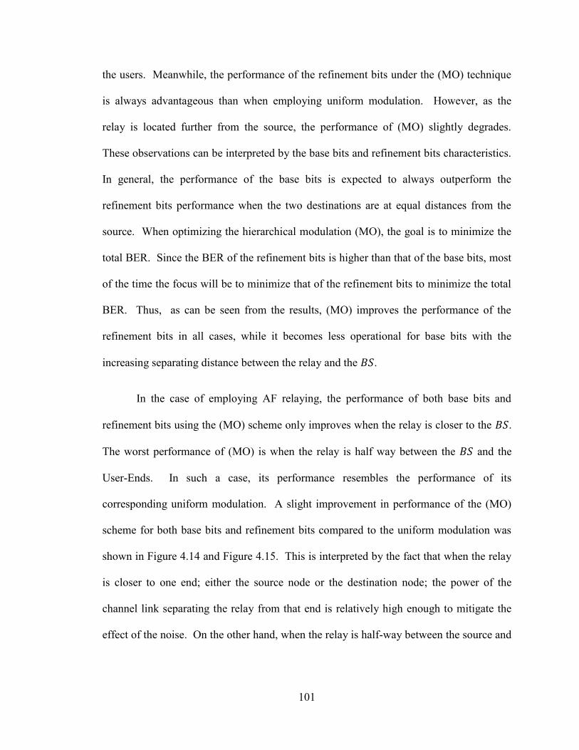
101
the users. Meanwhile, the performance of the refinement bits under the (MO) technique
is always advantageous than when employing uniform modulation. However, as the
relay is located further from the source, the performance of (MO) slightly degrades.
These observations can be interpreted by the base bits and refinement bits characteristics.
In general, the performance of the base bits is expected to always outperform the
refinement bits performance when the two destinations are at equal distances from the
source. When optimizing the hierarchical modulation (MO), the goal is to minimize the
total BER. Since the BER of the refinement bits is higher than that of the base bits, most
of the time the focus will be to minimize that of the refinement bits to minimize the total
BER. Thus, as can be seen from the results, (MO) improves the performance of the
refinement bits in all cases, while it becomes less operational for base bits with the
increasing separating distance between the relay and the .
In the case of employing AF relaying, the performance of both base bits and
refinement bits using the (MO) scheme only improves when the relay is closer to the .
The worst performance of (MO) is when the relay is half way between the and the
User-Ends. In such a case, its performance resembles the performance of its
corresponding uniform modulation. A slight improvement in performance of the (MO)
scheme for both base bits and refinement bits compared to the uniform modulation was
shown in Figure 4.14 and Figure 4.15. This is interpreted by the fact that when the relay
is closer to one end; either the source node or the destination node; the power of the
channel link separating the relay from that end is relatively high enough to mitigate the
effect of the noise. On the other hand, when the relay is half-way between the source and
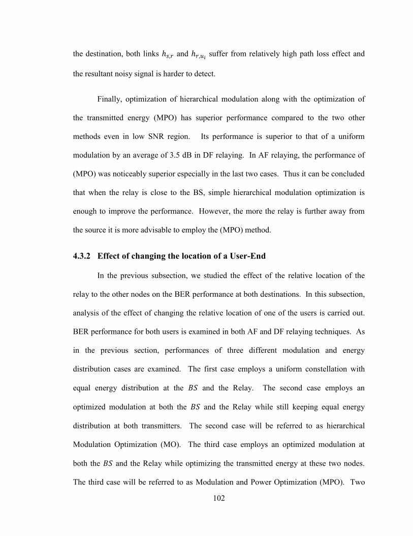
102
the destination, both links ℎ and ℎ suffer from relatively high path loss effect and
the resultant noisy signal is harder to detect.
Finally, optimization of hierarchical modulation along with the optimization of
the transmitted energy (MPO) has superior performance compared to the two other
methods even in low SNR region. Its performance is superior to that of a uniform
modulation by an average of 3.5 dB in DF relaying. In AF relaying, the performance of
(MPO) was noticeably superior especially in the last two cases. Thus it can be concluded
that when the relay is close to the BS, simple hierarchical modulation optimization is
enough to improve the performance. However, the more the relay is further away from
the source it is more advisable to employ the (MPO) method.
4.3.2 Effect of changing the location of a User-End
In the previous subsection, we studied the effect of the relative location of the
relay to the other nodes on the BER performance at both destinations. In this subsection,
analysis of the effect of changing the relative location of one of the users is carried out.
BER performance for both users is examined in both AF and DF relaying techniques. As
in the previous section, performances of three different modulation and energy
distribution cases are examined. The first case employs a uniform constellation with
equal energy distribution at the and the Relay. The second case employs an
optimized modulation at both the and the Relay while still keeping equal energy
distribution at both transmitters. The second case will be referred to as hierarchical
Modulation Optimization (MO). The third case employs an optimized modulation at
both the and the Relay while optimizing the transmitted energy at these two nodes.
The third case will be referred to as Modulation and Power Optimization (MPO). Two
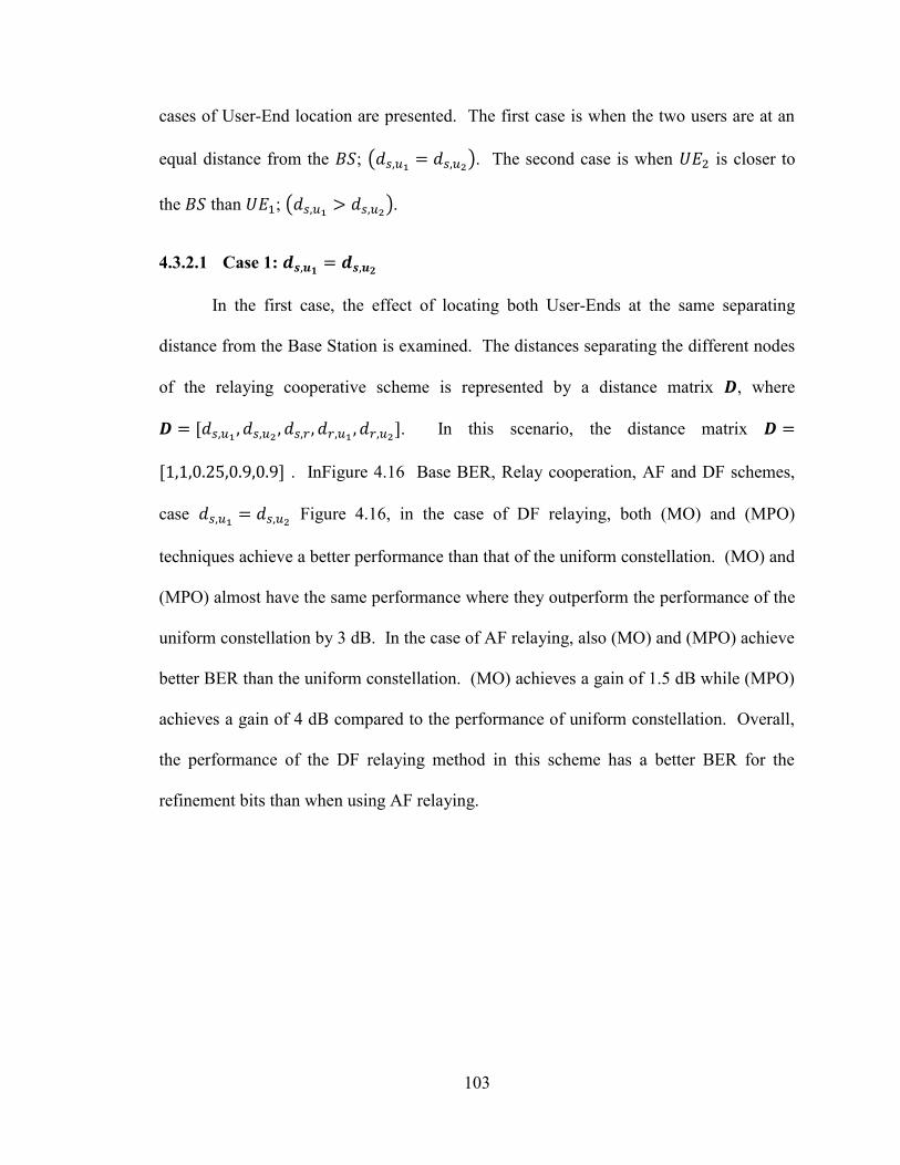
103
cases of User-End location are presented. The first case is when the two users are at an
equal distance from the ; (
). The second case is when is closer to
the than ; (
).
4.3.2.1 Case 1:
In the first case, the effect of locating both User-Ends at the same separating
distance from the Base Station is examined. The distances separating the different nodes
of the relaying cooperative scheme is represented by a distance matrix , where
[
]. In this scenario, the distance matrix
[ ] . InFigure 4.16 Base BER, Relay cooperation, AF and DF schemes,
case
Figure 4.16, in the case of DF relaying, both (MO) and (MPO)
techniques achieve a better performance than that of the uniform constellation. (MO) and
(MPO) almost have the same performance where they outperform the performance of the
uniform constellation by 3 dB. In the case of AF relaying, also (MO) and (MPO) achieve
better BER than the uniform constellation. (MO) achieves a gain of 1.5 dB while (MPO)
achieves a gain of 4 dB compared to the performance of uniform constellation. Overall,
the performance of the DF relaying method in this scheme has a better BER for the
refinement bits than when using AF relaying.
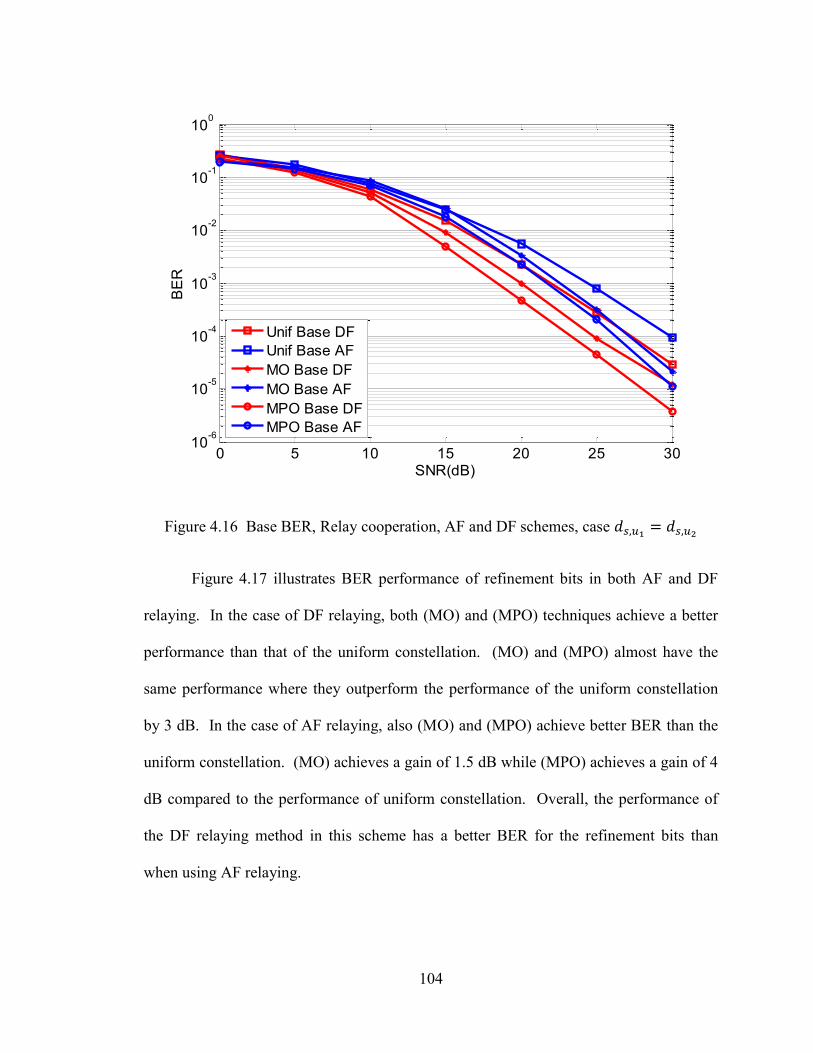
104
Figure 4.16 Base BER, Relay cooperation, AF and DF schemes, case
Figure 4.17 illustrates BER performance of refinement bits in both AF and DF
relaying. In the case of DF relaying, both (MO) and (MPO) techniques achieve a better
performance than that of the uniform constellation. (MO) and (MPO) almost have the
same performance where they outperform the performance of the uniform constellation
by 3 dB. In the case of AF relaying, also (MO) and (MPO) achieve better BER than the
uniform constellation. (MO) achieves a gain of 1.5 dB while (MPO) achieves a gain of 4
dB compared to the performance of uniform constellation. Overall, the performance of
the DF relaying method in this scheme has a better BER for the refinement bits than
when using AF relaying.
0 5 10 15 20 25 3010
-6
10-5
10-4
10-3
10-2
10-1
100
SNR(dB)
BE
R
Unif Base DF
Unif Base AF
MO Base DF
MO Base AF
MPO Base DF
MPO Base AF
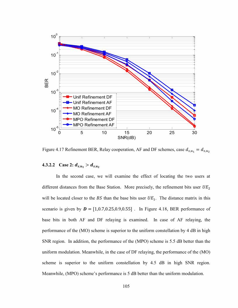
105
Figure 4.17 Refinement BER, Relay cooperation, AF and DF schemes, case
4.3.2.2 Case 2:
In the second case, we will examine the effect of locating the two users at
different distances from the Base Station. More precisely, the refinement bits user
will be located closer to the than the base bits user . The distance matrix in this
scenario is given by [ ] . In Figure 4.18, BER performance of
base bits in both AF and DF relaying is examined. In case of AF relaying, the
performance of the (MO) scheme is superior to the uniform constellation by 4 dB in high
SNR region. In addition, the performance of the (MPO) scheme is 5.5 dB better than the
uniform modulation. Meanwhile, in the case of DF relaying, the performance of the (MO)
scheme is superior to the uniform constellation by 4.5 dB in high SNR region.
Meanwhile, (MPO) scheme’s performance is 5 dB better than the uniform modulation.
0 5 10 15 20 25 3010
-5
10-4
10-3
10-2
10-1
100
SNR(dB)
BE
R
Unif Refinement DF
Unif Refinement AF
MO Refinement DF
MO Refinement AF
MPO Refinement DF
MPO Refinement AF
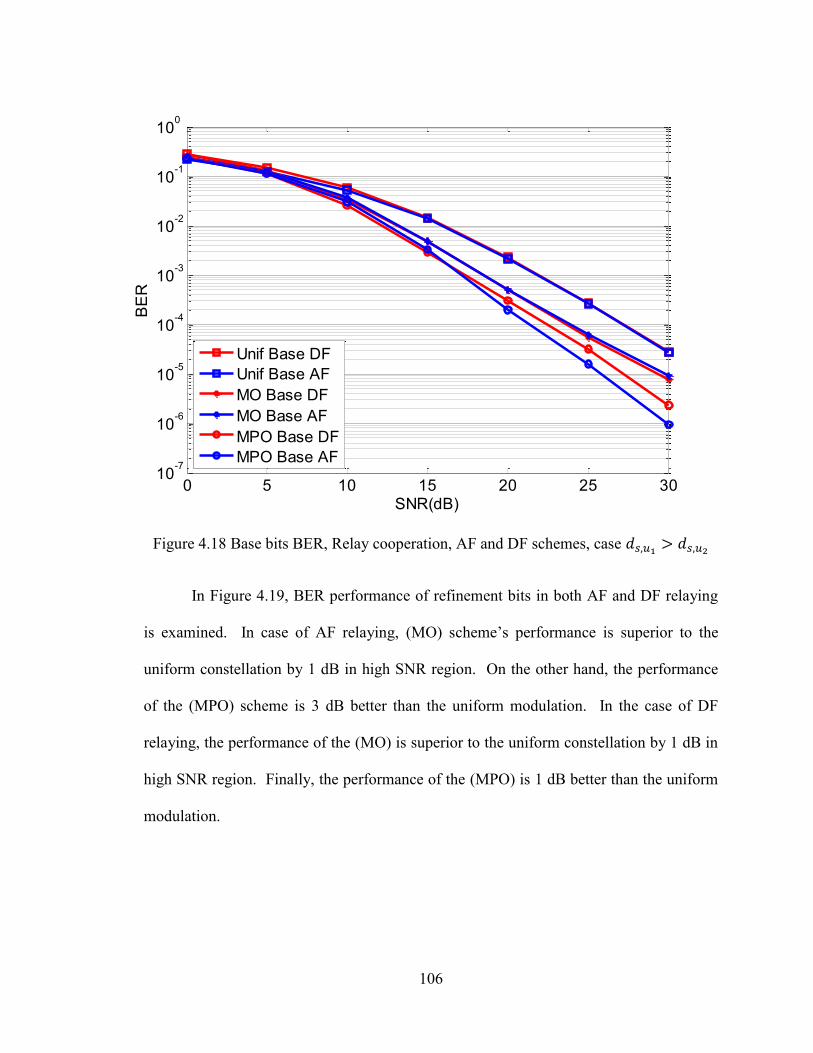
106
Figure 4.18 Base bits BER, Relay cooperation, AF and DF schemes, case
In Figure 4.19, BER performance of refinement bits in both AF and DF relaying
is examined. In case of AF relaying, (MO) scheme’s performance is superior to the
uniform constellation by 1 dB in high SNR region. On the other hand, the performance
of the (MPO) scheme is 3 dB better than the uniform modulation. In the case of DF
relaying, the performance of the (MO) is superior to the uniform constellation by 1 dB in
high SNR region. Finally, the performance of the (MPO) is 1 dB better than the uniform
modulation.
0 5 10 15 20 25 3010
-7
10-6
10-5
10-4
10-3
10-2
10-1
100
SNR(dB)
BE
R
Unif Base DF
Unif Base AF
MO Base DF
MO Base AF
MPO Base DF
MPO Base AF
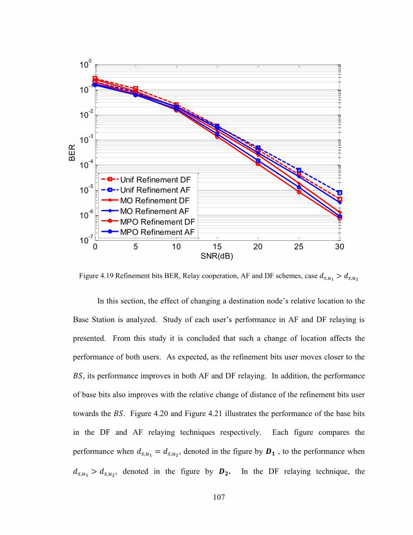
107
Figure 4.19 Refinement bits BER, Relay cooperation, AF and DF schemes, case
In this section, the effect of changing a destination node’s relative location to the
Base Station is analyzed. Study of each user’s performance in AF and DF relaying is
presented. From this study it is concluded that such a change of location affects the
performance of both users. As expected, as the refinement bits user moves closer to the
, its performance improves in both AF and DF relaying. In addition, the performance
of base bits also improves with the relative change of distance of the refinement bits user
towards the . Figure 4.20 and Figure 4.21 illustrates the performance of the base bits
in the DF and AF relaying techniques respectively. Each figure compares the
performance when
, denoted in the figure by , to the performance when
, denoted in the figure by . In the DF relaying technique, the
0 5 10 15 20 25 3010
-7
10-6
10-5
10-4
10-3
10-2
10-1
100
SNR(dB)
BE
R
Unif Refinement DF
Unif Refinement AF
MO Refinement DF
MO Refinement AF
MPO Refinement DF
MPO Refinement AF
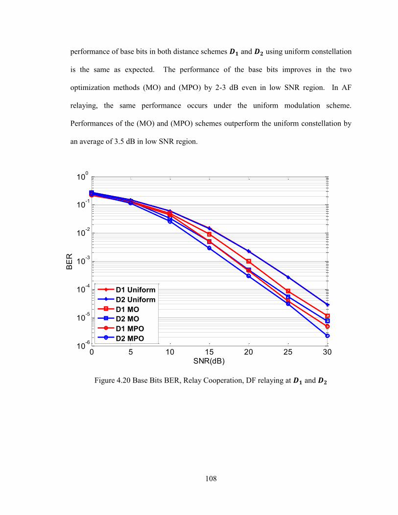
108
performance of base bits in both distance schemes and using uniform constellation
is the same as expected. The performance of the base bits improves in the two
optimization methods (MO) and (MPO) by 2-3 dB even in low SNR region. In AF
relaying, the same performance occurs under the uniform modulation scheme.
Performances of the (MO) and (MPO) schemes outperform the uniform constellation by
an average of 3.5 dB in low SNR region.
Figure 4.20 Base Bits BER, Relay Cooperation, DF relaying at and
0 5 10 15 20 25 3010
-6
10-5
10-4
10-3
10-2
10-1
100
SNR(dB)
BE
R
D1 Uniform
D2 Uniform
D1 MO
D2 MO
D1 MPO
D2 MPO
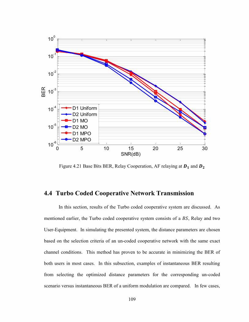
109
Figure 4.21 Base Bits BER, Relay Cooperation, AF relaying at and
4.4 Turbo Coded Cooperative Network Transmission
In this section, results of the Turbo coded cooperative system are discussed. As
mentioned earlier, the Turbo coded cooperative system consists of a , Relay and two
User-Equipment. In simulating the presented system, the distance parameters are chosen
based on the selection criteria of an un-coded cooperative network with the same exact
channel conditions. This method has proven to be accurate in minimizing the BER of
both users in most cases. In this subsection, examples of instantaneous BER resulting
from selecting the optimized distance parameters for the corresponding un-coded
scenario versus instantaneous BER of a uniform modulation are compared. In few cases,
0 5 10 15 20 25 3010
-6
10-5
10-4
10-3
10-2
10-1
100
SNR(dB)
BE
R
D1 Uniform
D2 Uniform
D1 MO
D2 MO
D1 MPO
D2 MPO
110
when the selected distance parameters are not optimum, they still achieve BER values
very close to the optimum ones. In addition, the overall performance of the system when
employing the proposed method is compared with the corresponding case of employing a
uniform 16QAM modulation.
4.4.1 Example 1
This example examines a Turbo relaying network at SNR = 5dB. The channel
coefficients between the components of this model are defined in channel matrix
[|ℎ | |ℎ
| |ℎ |
|ℎ
| |ℎ
| ]
In this example, [ ]. From the matrix
values it can be seen that the link is not powerful enough for the relay to decode
the message fully correctly. Thus, the users will only receive one copy of the data
coming from the . Using equations (3.8) and (3.9), and the values of |ℎ | and
|ℎ | , and can be computed to achieve the minimum total instantaneous BER.
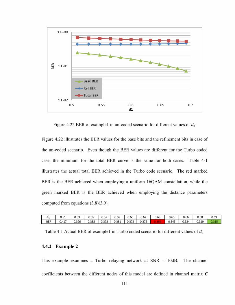
111
Figure 4.22 BER of example1 in un-coded scenario for different values of
Figure 4.22 illustrates the BER values for the base bits and the refinement bits in case of
the un-coded scenario. Even though the BER values are different for the Turbo coded
case, the minimum for the total BER curve is the same for both cases. Table 4-1
illustrates the actual total BER achieved in the Turbo code scenario. The red marked
BER is the BER achieved when employing a uniform 16QAM constellation, while the
green marked BER is the BER achieved when employing the distance parameters
computed from equations (3.8)(3.9).
Table 4-1 Actual BER of example1 in Turbo coded scenario for different values of
4.4.2 Example 2
This example examines a Turbo relaying network at SNR = 10dB. The channel
coefficients between the different nodes of this model are defined in channel matrix
0.51 0.53 0.55 0.57 0.58 0.60 0.62 0.63 0.65 0.66 0.68 0.69
BER 0.417 0.396 0.388 0.378 0.381 0.372 0.375 0.354 0.343 0.334 0.319 0.315
112
where [ ]. In this example, the link is
good enough for the relay to decode the message correctly. Thus, the users will
receive two copies of the data; one copy coming from the and the other coming from
the relay. Using equations (A.29) and (A.63), the values of the channel coefficients in
and the fact that ⁄ , the values of , , and can be computed
to achieve the minimum total instantaneous BER. Table 4-2 illustrates the total
computed instantaneous BER values in the case of the un-coded scenario. The red
marked BER is the total instantaneous BER in case of employing a uniform constellation.
The green marked BER is the minimum total instantaneous BER. This minimum value is
achieved when the constellation’s distance parameters set in the first time is {
} and when the constellation’s distance parameters set in the second time
slot is { }. Reflecting on the channel values in matrix , such a
choice of distance parameters is logical. As can be seen from the channel values, if we
consider the two channel links to ; |ℎ | |ℎ
| ; we will see
that the second link is more favorable. Thus, in the second time slot, the constellation’s
parameters are set to protect ’s data by increasing the value of . On the other
hand, considering the two channel links to ; |ℎ | |ℎ
| ; we
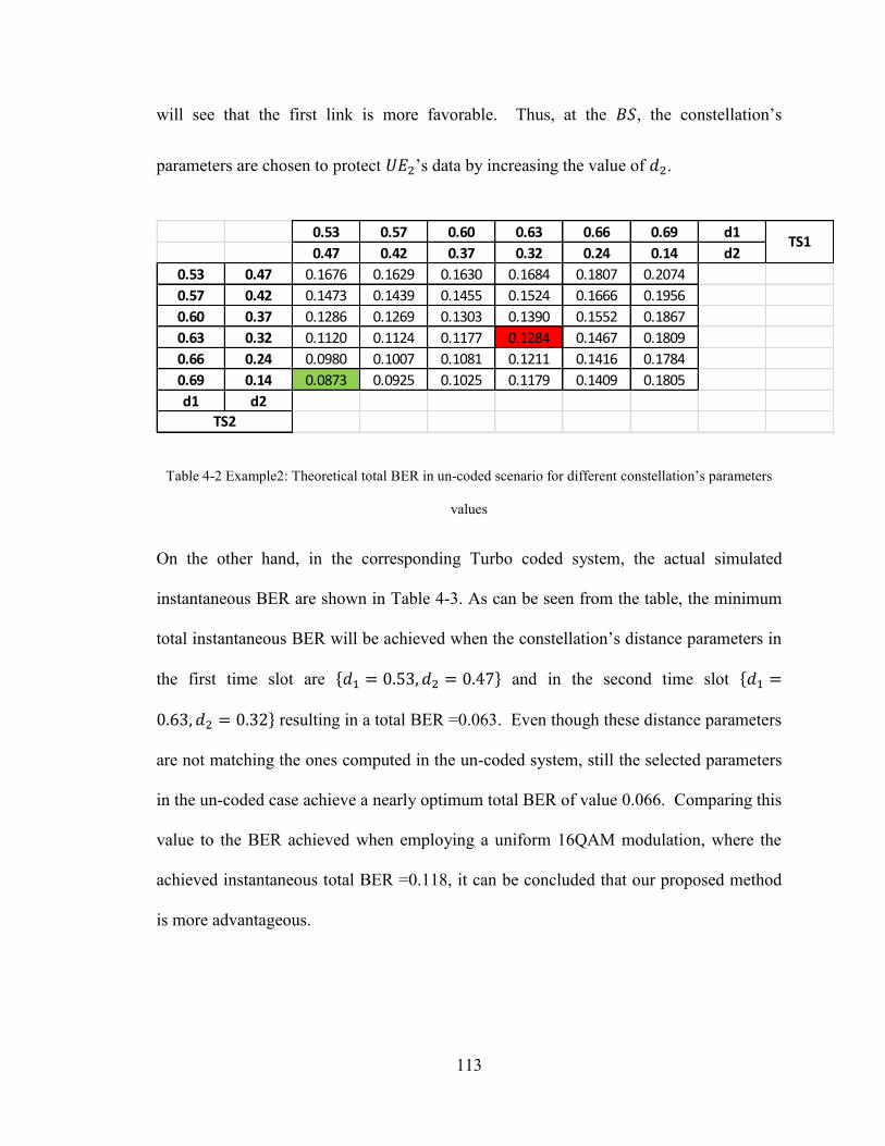
113
will see that the first link is more favorable. Thus, at the , the constellation’s
parameters are chosen to protect ’s data by increasing the value of .
Table 4-2 Example2: Theoretical total BER in un-coded scenario for different constellation’s parameters
values
On the other hand, in the corresponding Turbo coded system, the actual simulated
instantaneous BER are shown in Table 4-3. As can be seen from the table, the minimum
total instantaneous BER will be achieved when the constellation’s distance parameters in
the first time slot are { } and in the second time slot {
} resulting in a total BER =0.063. Even though these distance parameters
are not matching the ones computed in the un-coded system, still the selected parameters
in the un-coded case achieve a nearly optimum total BER of value 0.066. Comparing this
value to the BER achieved when employing a uniform 16QAM modulation, where the
achieved instantaneous total BER =0.118, it can be concluded that our proposed method
is more advantageous.
0.53 0.57 0.60 0.63 0.66 0.69 d1
0.47 0.42 0.37 0.32 0.24 0.14 d2
0.53 0.47 0.1676 0.1629 0.1630 0.1684 0.1807 0.2074
0.57 0.42 0.1473 0.1439 0.1455 0.1524 0.1666 0.1956
0.60 0.37 0.1286 0.1269 0.1303 0.1390 0.1552 0.1867
0.63 0.32 0.1120 0.1124 0.1177 0.1284 0.1467 0.1809
0.66 0.24 0.0980 0.1007 0.1081 0.1211 0.1416 0.1784
0.69 0.14 0.0873 0.0925 0.1025 0.1179 0.1409 0.1805
d1 d2
TS1
TS2
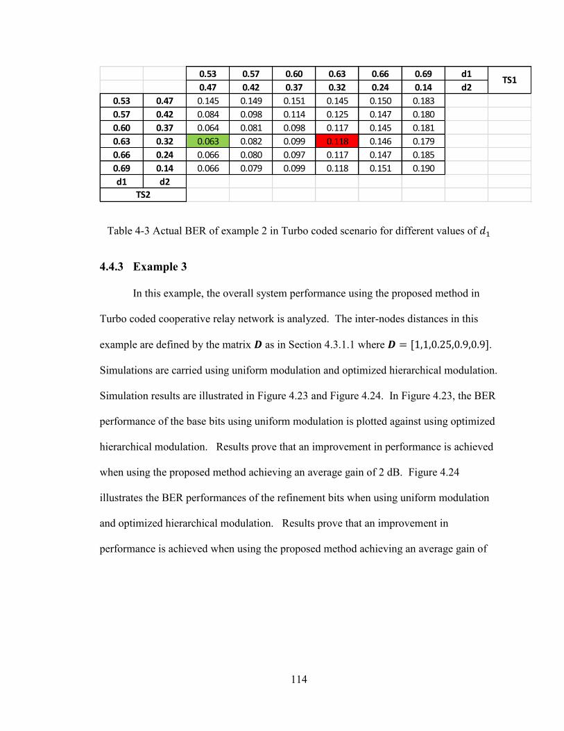
114
Table 4-3 Actual BER of example 2 in Turbo coded scenario for different values of
4.4.3 Example 3
In this example, the overall system performance using the proposed method in
Turbo coded cooperative relay network is analyzed. The inter-nodes distances in this
example are defined by the matrix as in Section 4.3.1.1 where [ ].
Simulations are carried using uniform modulation and optimized hierarchical modulation.
Simulation results are illustrated in Figure 4.23 and Figure 4.24. In Figure 4.23, the BER
performance of the base bits using uniform modulation is plotted against using optimized
hierarchical modulation. Results prove that an improvement in performance is achieved
when using the proposed method achieving an average gain of 2 dB. Figure 4.24
illustrates the BER performances of the refinement bits when using uniform modulation
and optimized hierarchical modulation. Results prove that an improvement in
performance is achieved when using the proposed method achieving an average gain of
0.53 0.57 0.60 0.63 0.66 0.69 d1
0.47 0.42 0.37 0.32 0.24 0.14 d2
0.53 0.47 0.145 0.149 0.151 0.145 0.150 0.183
0.57 0.42 0.084 0.098 0.114 0.125 0.147 0.180
0.60 0.37 0.064 0.081 0.098 0.117 0.145 0.181
0.63 0.32 0.063 0.082 0.099 0.118 0.146 0.179
0.66 0.24 0.066 0.080 0.097 0.117 0.147 0.185
0.69 0.14 0.066 0.079 0.099 0.118 0.151 0.190
d1 d2
TS2
TS1
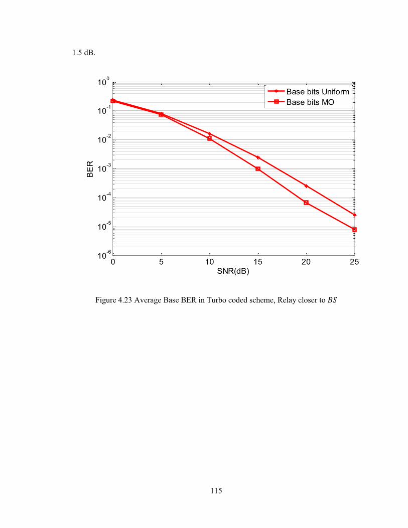
115
1.5 dB.
Figure 4.23 Average Base BER in Turbo coded scheme, Relay closer to
0 5 10 15 20 2510
-6
10-5
10-4
10-3
10-2
10-1
100
SNR(dB)
BE
R
Base bits Uniform
Base bits MO
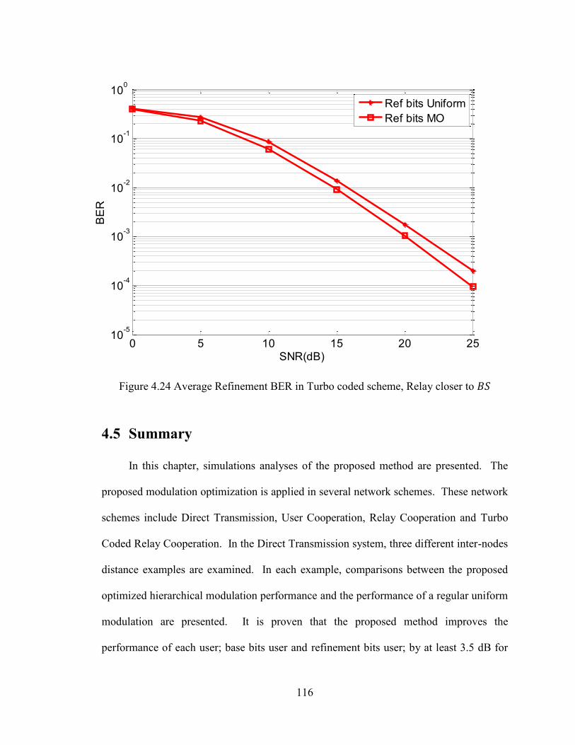
116
Figure 4.24 Average Refinement BER in Turbo coded scheme, Relay closer to
4.5 Summary
In this chapter, simulations analyses of the proposed method are presented. The
proposed modulation optimization is applied in several network schemes. These network
schemes include Direct Transmission, User Cooperation, Relay Cooperation and Turbo
Coded Relay Cooperation. In the Direct Transmission system, three different inter-nodes
distance examples are examined. In each example, comparisons between the proposed
optimized hierarchical modulation performance and the performance of a regular uniform
modulation are presented. It is proven that the proposed method improves the
performance of each user; base bits user and refinement bits user; by at least 3.5 dB for
0 5 10 15 20 2510
-5
10-4
10-3
10-2
10-1
100
SNR(dB)
BE
R
Ref bits Uniform
Ref bits MO
117
base bits user and 1.5 dB for refinement bits user. It is also concluded that under
hierarchical modulation application, the change in one user’s location affects the
performance of both users.
In the case of user cooperation, two examples are presented. The first example
evaluates the efficiency of optimized hierarchical modulation when the correct reception
of one user’s data ( ’s data) is more important than the other user’s data ( ’s data).
In this case, relays the data it receives belonging to when possible. This
solution outperforms the use of simple Direct Transmission employing uniform
modulation scheme by 5 dB. Also optimized hierarchical modulation in this scheme
outperforms its corresponding uniform modulation by 2dB. In the second example, the
user with advantageous channel condition assists the user with less favorable channel
condition to better detect its data. In that scheme, the proposed method outperforms its
corresponding uniform modulation by at least 2dB.
In relay cooperative network scheme, system evaluations of different relative Relay
locations in the network are carried out. It is concluded that the best performance of the
suggested scheme is when the relay is located closer to the Base Station. Simulation
results vary depending on the relaying protocol used; AF or DF. In DF relaying, the
performance of the proposed method is less efficient when the relay is further located
from the Base Station. On the other hand in AF relaying, the performance of the
proposed system is worst when the relay is located half way between the Base Station
and the users. Adjusting the total transmitted energy among the transmitters is also
examined in the Relay cooperative scheme. It is shown that such adjustment along with
the proposed hierarchical modulation optimization result in even better performances of
118
both users. In the second part of the Relay cooperative system results, a study on varying
the location of one of the User Equipment is carried out. In the case where uniform
modulation is used, only the user with changing location experiences different BER
performances. However, in the case where optimized modulation is used, the
performance of both users is affected.
Finally, the presented study is extended to analyse the application of the proposed
system in the Turbo coded relay cooperative network environment. In this model,
instantaneous selected constellation’s parameters are tested to achieve minimum or
almost minimum total instantaneous BER. Two examples are presented where it is
proven that the proposed method achieves near optimum instantaneous BER values. In
the third example, the average total BER for base bits and refinement bits achieved using
optimized hierarchical modulation is plotted versus the corresponding achieved BER
using uniform modulation. It is shown that for both users improvement in BER
performance is achieved when optimized hierarchical modulation is employed.
119
Chapter Five
Conclusion and Future work 5.
Recently, the use of higher order modulation in cooperative networks has acquired
special interest in the research field. High order modulations have the capability of
transmitting higher data rate than just simple binary modulation. Thus they are more
desirable in cooperative network environments to mitigate the need for extra bandwidth.
The hierarchical 4/16-QAM modulation is one of the most extensively studied and
practically employed in the field of wireless networks due to its simplicity and moderate
compromise between performance and data rate.
In this thesis, an adjustable 4/16 QAM hierarchical modulation is developed. It
adjusts its distributed energy among the receivers according to the channel condition
120
linking to each user. We apply our proposed protocol to downlink cellular network with
a cooperative relay. In this system model, the Base Station aims at delivering two
different messages to two different users by concatenating their data together using a 4/16
QAM modulation. The goal of the system is to adjust the modulation parameters in order
to minimize the total BER. In order to optimize the hierarchical modulation parameters,
theoretical BER for each user in direct transmission and cooperative relay transmission;
including AF and DF protocol; are derived in this thesis. Full channel knowledge at all
nodes is assumed before transmission. Unlike previous developed systems, the
optimization of the hierarchical modulation in this thesis is based on the channel
conditions carrying the transmitted data. This resulted in improved performance for all
destinations compared to previous work that generally focused on improving the
performance only at one User Equipment.
In Chapter 3, the system model studied in this thesis is explained. Different
scenarios of transmission have been presented including direct transmission, cooperative
transmission and coded cooperative transmission. All related system parameters are
explained in details including the modulation/demodulation and encoding/decoding
factors. In Chapter 4, simulation results of the different designed schemes are presented.
In direct transmission, the use of our proposed system always outperforms the use of
uniform modulation. The improvement in performance is even more noticeable when the
two destinations are unequally distant from the source. User cooperation simulations
improve the performance of users experiencing unfavorable channel conditions.
Employment of adjustable hierarchical modulation in this model outperforms its uniform
modulation counterpart. In relay cooperative model, several relay locations and user
121
locations are studied, where optimized hierarchical modulation shows to be more
efficient in situations than in others. But overall, adjusting the transmitted energy on the
transmitters while adjusting the hierarchical modulation energy always show noticeable
performance improvement for both destinations. Lastly, our proposed method is
extended to Turbo coded cooperative network scenario. The use of theoretically derived
optimized modulation parameters for un-coded cooperative environment in Turbo coded
cooperative environment is tested. Even though this method may not be optimum all the
time, it has proven to improve the performance in most cases and has led to overall
improvement in the performance of the User Equipment.
Currently, this specific topic is still under preliminary research. There are a couple
of ways in which future work can be conducted for this topic. First, investigation of the
performance of optimized high order modulation in other cooperative network topologies
such as bidirectional relay networks, or uplink topology can be conducted. Second,
computations of actual theoretical BER of base bits and refinement bits in Turbo coded
relay cooperative networks can be carried on in future work in order to improve the
performance of hierarchical modulation in such an environment. Overall, this is a
promising research topic that has proven in this work to achieve a worthwhile
performance improvement.
122
A. Appendix
A.1 Hierarchical modulation BER computation in a
Rayleigh fading cooperative network using
MRC
In this section, theoretical derivations of the instantaneous BER for the base bits
and the refinement bits in a 4/16 QAM constellation in DF and AF relaying using
MRC combining technique in Rayleigh fading environment are presented. These
derivations are very vital in this work. In the modulation process, these expressions are
used to choose the constellation’s parameters that will minimize the total BER. In this
thesis, the same strategy applied in [68] [105] is followed to derive the required BER
expressions.
In this Chapter, the scenario in each relaying technique is briefly explained. In
this work, only DF and AF relaying methods are considered. Then the technique for
123
deriving the probability of error of base and refinement bits for each of these relaying
methods is explained.
In the Decode and Forward (DF) scenario, the signal is decoded at the relay and a
CRC check is applied. If the CRC check fails, the relay remains silent and the users
receive their data only from the Base Station. Only in the case of a correct reception of
a whole block of transmitted signals, i.e. the CRC check succeeded, these signals are
re-modulated and retransmitted with the corresponding constellation distance
parameters. At the destination, the signals coming from the Base Station and from the
relay are added together using MRC and a hard decision threshold is applied. It is to
be noted that in the DF relaying scenario, the constellation’s distance parameters
chosen during the modulation process at the Base Station can be different from those
chosen at the relay.
In the Amplify and Forward (AF) scenario, the signal is amplified at the relay by a
certain amplifying gain factor and is re-broadcasted to the other nodes without any
further processing. At each destination, the signals coming from the Base Station and
from the relay are added together and a hard decision threshold is applied. In AF
relaying scheme, the same constellation’s distance parameters are used during
modulation at the Base Station and the relay.
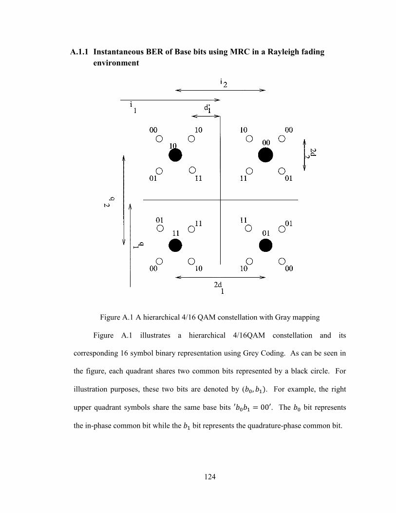
124
A.1.1 Instantaneous BER of Base bits using MRC in a Rayleigh fading
environment
Figure A.1 A hierarchical 4/16 QAM constellation with Gray mapping
Figure A.1 illustrates a hierarchical 4/16QAM constellation and its
corresponding 16 symbol binary representation using Grey Coding. As can be seen in
the figure, each quadrant shares two common bits represented by a black circle. For
illustration purposes, these two bits are denoted by ( . For example, the right
upper quadrant symbols share the same base bits . The bit represents
the in-phase common bit while the bit represents the quadrature-phase common bit.
125
Let’s consider sending a ‘0’ on the bit , the probability of getting an error, i.e.
the reception of a ‘1’, means that the resulting signal of combining the two signals
coming from the BS and from the relay; denoted by ; resulted in a reception of signal
in the negative side of the y axis. Thus the probability of receiving in error can be
expressed as:
(A.1)
In the case of receiving ; the quadrature phase bit; in error, only the imaginary
part of will be considered. In this study, only the error probability computations of
the in-phase common bit are considered. However, error probability computations
for the quadrature phase common bit are straight forward. In all the coming
computations, all real part notations will be omitted for simplification (i.e.
).
Let’s assume that the symbol is sent, which in the 4/16 QAM
constellation in Figure A.1 is situated at a distance from the axis.
Recalling from Chapter3, Equation (3.4), the modulated symbol in this specific case
will be . The received signals in the first time slot at the destination and at
the relay from the Base Station can be written respectively as
√ ℎ (A.2)
√ ℎ (A.3)
126
In the above equations, is the transmitting energy per symbol at the Base Station,
ℎ and ℎ are the fading channel coefficients on the source-destination link and the
source-relay link respectively. and are the AWGN coefficient at the destination
and at the relay respectively. denote the selected distance parameters in the first
time slot.
a) DF Relaying Case
If the CRC check results in successful decoding, the relay re-modulates its signal with
new constellation’s distance parameters and re-sends its signal. At the destination, the
received signal from the relay is expressed as
√
ℎ (A.4)
is the transmitted energy per symbol at the relay, ℎ is the fading channel
coefficient on the relay-destination link and is the AWGN coefficient at the
destination.
denote the selected distance parameters in the second time slot.
The two signals and are combined at the destination using MRC
technique. In this technique, each signal is weighted by its channel coefficient and the
two signals are added together. The resultant signal is given by:
√ |ℎ | ℎ
√
|ℎ |
ℎ
(A.5)
Thus, from equations (A.1) and (A.5) the probability of error for the bit in the symbol
can be written as follow:
127
([√ |ℎ | ℎ
√
|ℎ |
ℎ ] )
(A.6)
([√ |ℎ | √
|ℎ |
]
ℎ ℎ
)
(A.7)
Let’s denote ℎ ℎ
, where ( (|ℎ |
|ℎ | )). Also, let [√ |ℎ |
√
|ℎ |
]. Using these
notations, equation (A.7) can be written as
∫
√
(
)
let
∫
√
(
) (A.8)
Thus the instantaneous probability of bit error for common bits (base bits) given that the
symbol was sent using DF relaying over Rayleigh fading channel can be
expressed by:
128
(
[√ |ℎ |
√
|ℎ |
]
√|ℎ | |ℎ |
)
(A.9)
b) AF relaying Case
In the case of relaying the signal using Amplify and Forward, the relay amplifies the
received signal by a gain factor , where √
| |
and is the
transmitting energy at the relay, is the transmitting energy at the Base Station and
is the noise power spectral density. After the relay amplifies the signal and re-sends it,
the received signal at the destination from the relay is given by
ℎ (A.10)
ℎ ℎ √ ℎ
(A.11)
where ℎ is the fading channel coefficient on the relay-destination link and is the
AWGN coefficient at the destination. The two signals and are combined at the
destination using MRC technique. The resultant signal is given by:
√ |ℎ | ℎ
√ |ℎ | |ℎ |
|ℎ | ℎ ℎ
ℎ
(A.12)
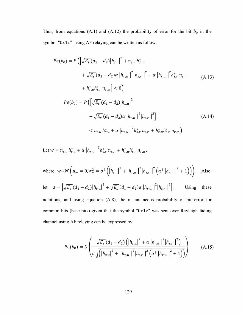
129
Thus, from equations (A.1) and (A.12) the probability of error for the bit in the
symbol using AF relaying can be written as follow:
([√ |ℎ | ℎ
√ |ℎ | |ℎ |
|ℎ |
ℎ
ℎ ℎ
] )
(A.13)
([√ |ℎ |
√ |ℎ | |ℎ |
]
ℎ |ℎ |
ℎ ℎ
ℎ )
(A.14)
Let ℎ |ℎ |
ℎ ℎ
ℎ ,
where ( (|ℎ |
|ℎ |
|ℎ |
( |ℎ |
))). Also,
let [√ |ℎ | √ |ℎ |
|ℎ |
]. Using these
notations, and using equation (A.8), the instantaneous probability of bit error for
common bits (base bits) given that the symbol was sent over Rayleigh fading
channel using AF relaying can be expressed by:
(
√ (|ℎ |
|ℎ |
|ℎ |
)
√(|ℎ | |ℎ |
|ℎ |
( |ℎ |
))
)
(A.15)
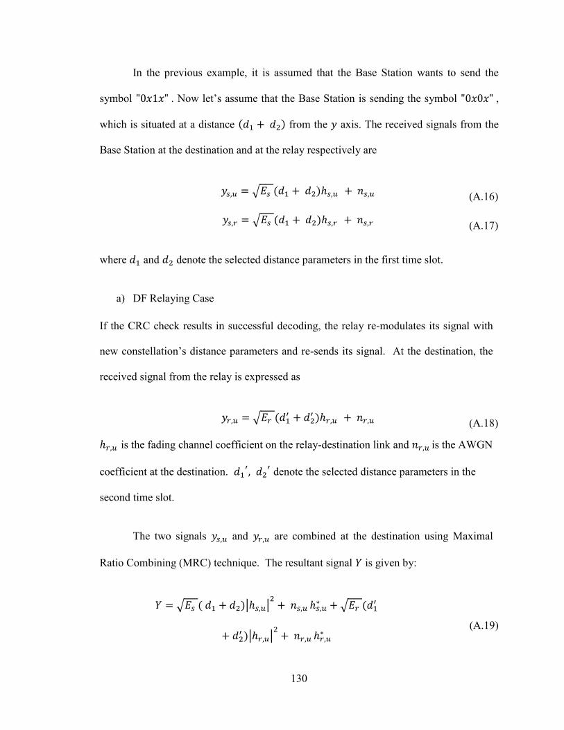
130
In the previous example, it is assumed that the Base Station wants to send the
symbol . Now let’s assume that the Base Station is sending the symbol ,
which is situated at a distance from the axis. The received signals from the
Base Station at the destination and at the relay respectively are
√ ℎ (A.16)
√ ℎ (A.17)
where and denote the selected distance parameters in the first time slot.
a) DF Relaying Case
If the CRC check results in successful decoding, the relay re-modulates its signal with
new constellation’s distance parameters and re-sends its signal. At the destination, the
received signal from the relay is expressed as
√
ℎ (A.18)
ℎ is the fading channel coefficient on the relay-destination link and is the AWGN
coefficient at the destination.
denote the selected distance parameters in the
second time slot.
The two signals and are combined at the destination using Maximal
Ratio Combining (MRC) technique. The resultant signal is given by:
√ |ℎ | ℎ
√
|ℎ |
ℎ
(A.19)
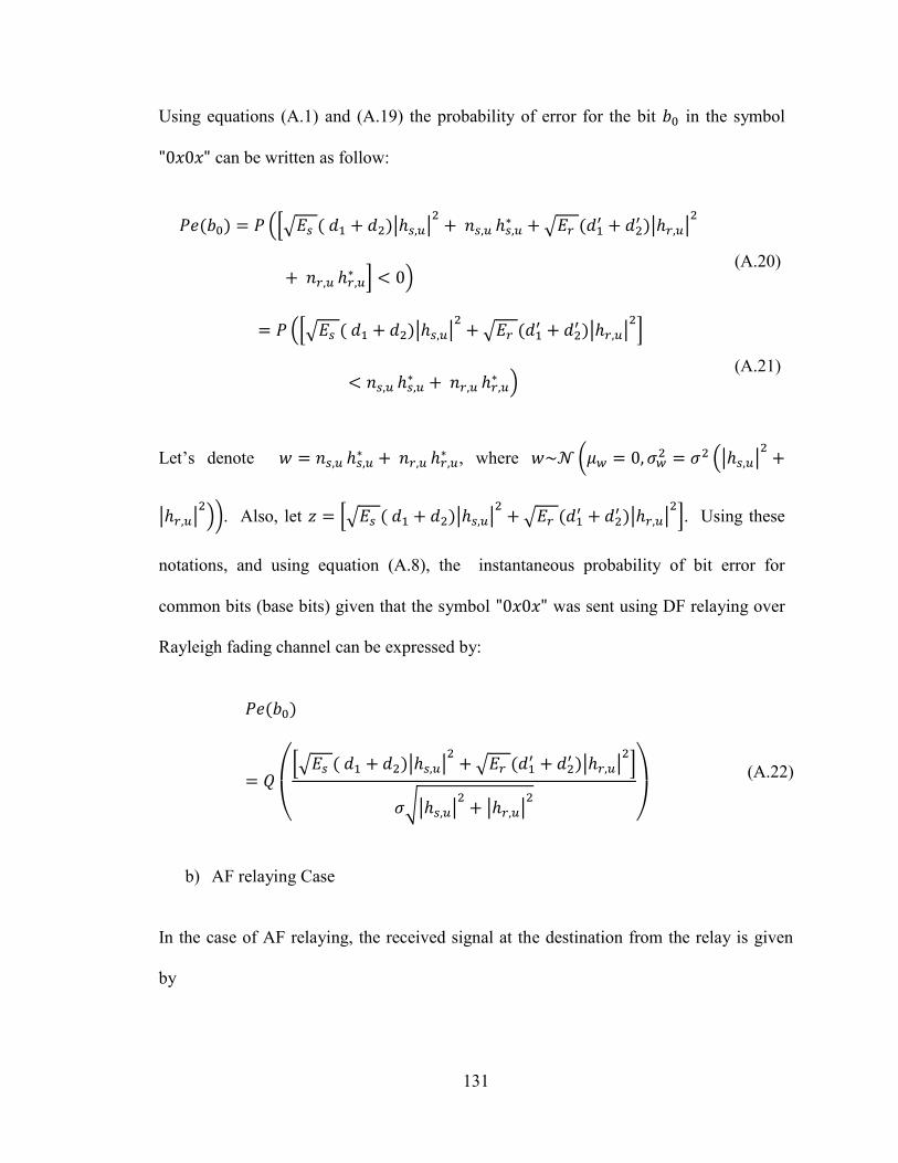
131
Using equations (A.1) and (A.19) the probability of error for the bit in the symbol
can be written as follow:
([√ |ℎ | ℎ
√
|ℎ |
ℎ ] )
(A.20)
([√ |ℎ | √
|ℎ |
]
ℎ ℎ
)
(A.21)
Let’s denote ℎ ℎ
, where ( (|ℎ |
|ℎ | )). Also, let [√ |ℎ |
√
|ℎ |
]. Using these
notations, and using equation (A.8), the instantaneous probability of bit error for
common bits (base bits) given that the symbol was sent using DF relaying over
Rayleigh fading channel can be expressed by:
(
[√ |ℎ |
√
|ℎ |
]
√|ℎ | |ℎ |
)
(A.22)
b) AF relaying Case
In the case of AF relaying, the received signal at the destination from the relay is given
by
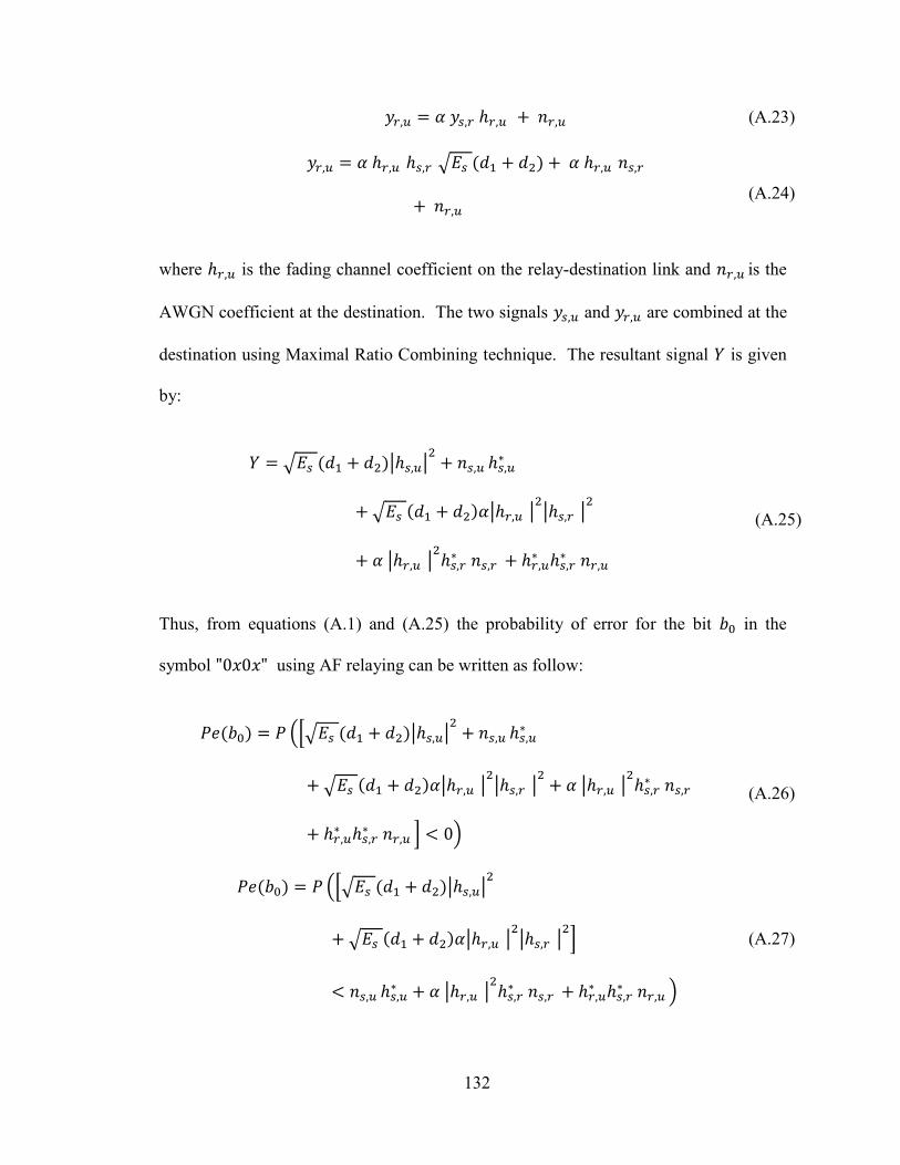
132
ℎ (A.23)
ℎ ℎ √ ℎ
(A.24)
where ℎ is the fading channel coefficient on the relay-destination link and is the
AWGN coefficient at the destination. The two signals and are combined at the
destination using Maximal Ratio Combining technique. The resultant signal is given
by:
√ |ℎ | ℎ
√ |ℎ | |ℎ |
|ℎ | ℎ ℎ
ℎ
(A.25)
Thus, from equations (A.1) and (A.25) the probability of error for the bit in the
symbol using AF relaying can be written as follow:
([√ |ℎ | ℎ
√ |ℎ | |ℎ |
|ℎ |
ℎ
ℎ ℎ
] )
(A.26)
([√ |ℎ |
√ |ℎ | |ℎ |
]
ℎ |ℎ |
ℎ ℎ
ℎ )
(A.27)
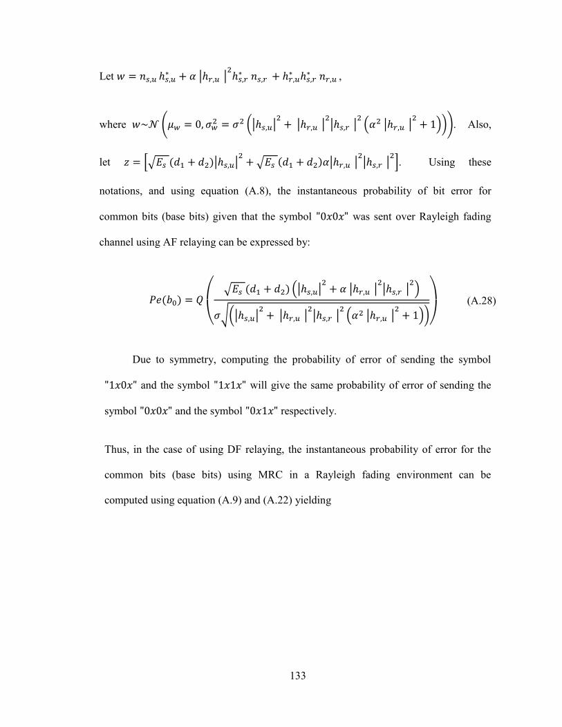
133
Let ℎ |ℎ |
ℎ ℎ
ℎ ,
where ( (|ℎ |
|ℎ |
|ℎ |
( |ℎ |
))). Also,
let [√ |ℎ | √ |ℎ |
|ℎ |
]. Using these
notations, and using equation (A.8), the instantaneous probability of bit error for
common bits (base bits) given that the symbol was sent over Rayleigh fading
channel using AF relaying can be expressed by:
(
√ (|ℎ |
|ℎ |
|ℎ |
)
√(|ℎ | |ℎ |
|ℎ |
( |ℎ |
))
)
(A.28)
Due to symmetry, computing the probability of error of sending the symbol
and the symbol will give the same probability of error of sending the
symbol and the symbol respectively.
Thus, in the case of using DF relaying, the instantaneous probability of error for the
common bits (base bits) using MRC in a Rayleigh fading environment can be
computed using equation (A.9) and (A.22) yielding
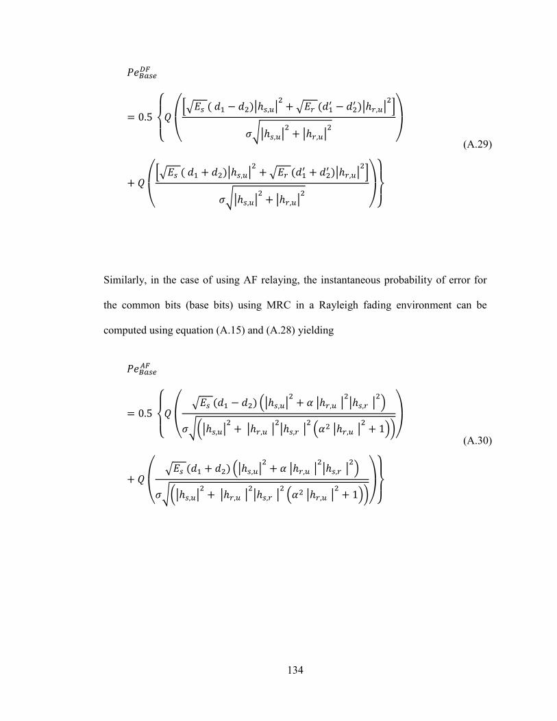
134
{
(
[√ |ℎ |
√
|ℎ |
]
√|ℎ | |ℎ |
)
(
[√ |ℎ |
√
|ℎ |
]
√|ℎ | |ℎ |
)
}
(A.29)
Similarly, in the case of using AF relaying, the instantaneous probability of error for
the common bits (base bits) using MRC in a Rayleigh fading environment can be
computed using equation (A.15) and (A.28) yielding
{
(
√ (|ℎ |
|ℎ |
|ℎ |
)
√(|ℎ | |ℎ |
|ℎ |
( |ℎ |
))
)
(
√ (|ℎ |
|ℎ |
|ℎ |
)
√(|ℎ | |ℎ |
|ℎ |
( |ℎ |
))
)
}
(A.30)
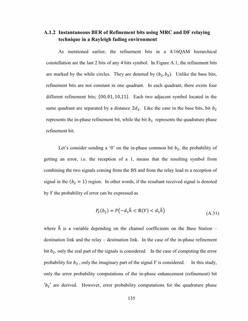
135
A.1.2 Instantaneous BER of Refinement bits using MRC and DF relaying
technique in a Rayleigh fading environment
As mentioned earlier, the refinement bits in a 4/16QAM hierarchical
constellation are the last 2 bits of any 4 bits symbol. In Figure A.1, the refinement bits
are marked by the while circles. They are denoted by ( . Unlike the base bits,
refinement bits are not constant in one quadrant. In each quadrant, there exists four
different refinement bits; { }. Each two adjacent symbol located in the
same quadrant are separated by a distance . Like the case in the base bits, bit
represents the in-phase refinement bit, while the bit represents the quadrature phase
refinement bit.
Let’s consider sending a ‘0’ on the in-phase common bit , the probability of
getting an error, i.e. the reception of a 1, means that the resulting symbol from
combining the two signals coming from the BS and from the relay lead to a reception of
signal in the region. In other words, if the resultant received signal is denoted
by the probability of error can be expressed as
( ℎ ℎ) (A.31)
where ℎ is a variable depending on the channel coefficients on the Base Station –
destination link and the relay – destination link. In the case of the in-phase refinement
bit , only the real part of the signals is considered. In the case of computing the error
probability for , only the imaginary part of the signal is considered. In this study,
only the error probability computations of the in-phase enhancement (refinement) bit
are derived. However, error probability computations for the quadrature phase
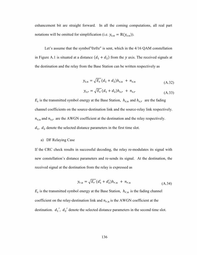
136
enhancement bit are straight forward. In all the coming computations, all real part
notations will be omitted for simplification (i.e. ).
Let’s assume that the symbol is sent, which in the 4/16 QAM constellation
in Figure A.1 is situated at a distance from the axis. The received signals at
the destination and the relay from the Base Station can be written respectively as
√ ℎ (A.32)
√ ℎ (A.33)
is the transmitted symbol energy at the Base Station, ℎ and ℎ are the fading
channel coefficients on the source-destination link and the source-relay link respectively.
and are the AWGN coefficient at the destination and the relay respectively.
denote the selected distance parameters in the first time slot.
a) DF Relaying Case
If the CRC check results in successful decoding, the relay re-modulates its signal with
new constellation’s distance parameters and re-sends its signal. At the destination, the
received signal at the destination from the relay is expressed as
√
ℎ (A.34)
is the transmitted symbol energy at the Base Station, ℎ is the fading channel
coefficient on the relay-destination link and is the AWGN coefficient at the
destination.
denote the selected distance parameters in the second time slot.
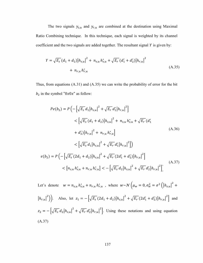
137
The two signals and are combined at the destination using Maximal
Ratio Combining technique. In this technique, each signal is weighted by its channel
coefficient and the two signals are added together. The resultant signal is given by:
√ |ℎ |
ℎ
√
|ℎ |
ℎ
(A.35)
Thus, from equations (A.31) and (A.35) we can write the probability of error for the bit
in the symbol as follow:
( [√ |ℎ | √
|ℎ | ]
[√ |ℎ | ℎ
√
|ℎ |
ℎ
]
[√ |ℎ | √
|ℎ | ])
(A.36)
( [√ |ℎ | √
|ℎ |
]
[ ℎ ℎ
] [√ |ℎ | √
|ℎ | ])
(A.37)
Let’s denote ℎ ℎ
, where ( (|ℎ |
|ℎ | )). Also, let [√ |ℎ |
√
|ℎ |
] and
[√ |ℎ | √
|ℎ | ]. Using these notations and using equation
(A.37)
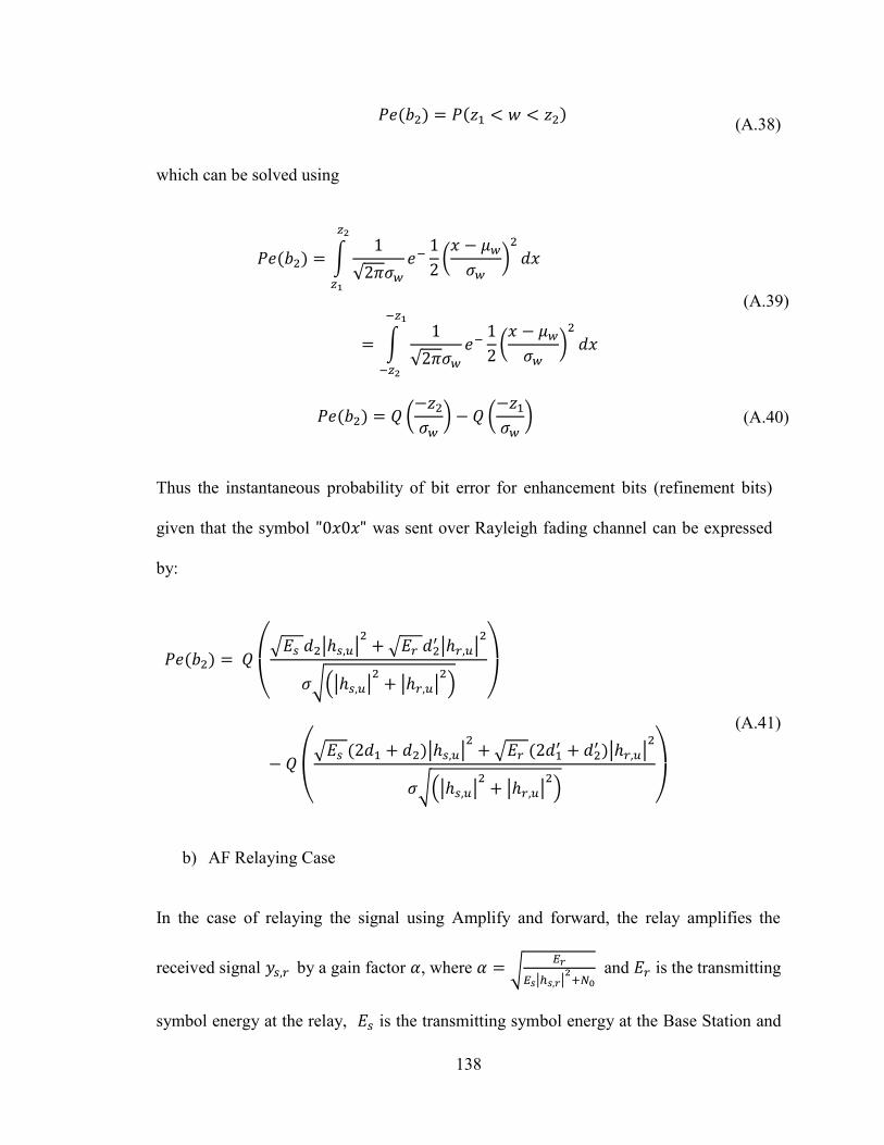
138
(A.38)
which can be solved using
∫
√
(
)
∫
√
(
)
(A.39)
(
) (
) (A.40)
Thus the instantaneous probability of bit error for enhancement bits (refinement bits)
given that the symbol was sent over Rayleigh fading channel can be expressed
by:
(
√ |ℎ |
√
|ℎ |
√(|ℎ | |ℎ |
)
)
(
√ |ℎ |
√
|ℎ |
√(|ℎ | |ℎ |
)
)
(A.41)
b) AF Relaying Case
In the case of relaying the signal using Amplify and forward, the relay amplifies the
received signal by a gain factor , where √
| |
and is the transmitting
symbol energy at the relay, is the transmitting symbol energy at the Base Station and
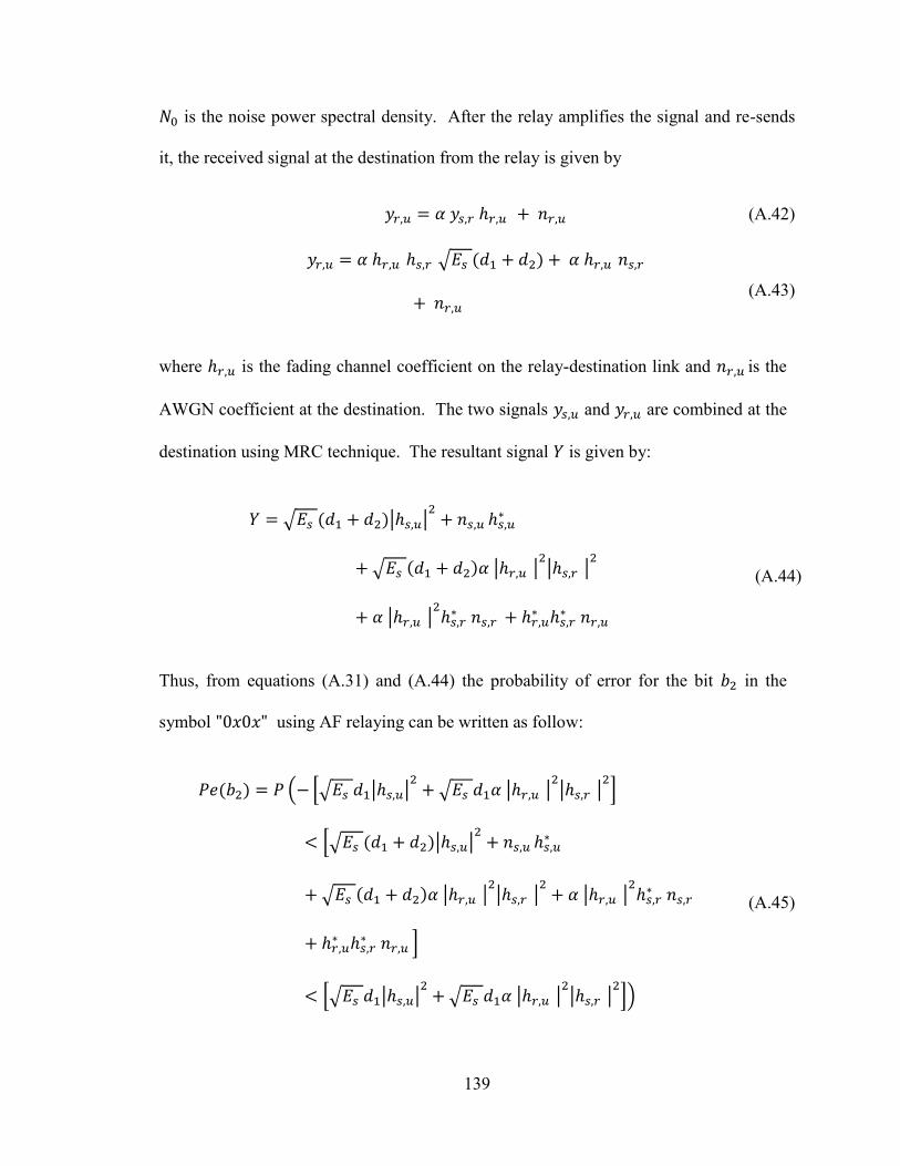
139
is the noise power spectral density. After the relay amplifies the signal and re-sends
it, the received signal at the destination from the relay is given by
ℎ (A.42)
ℎ ℎ √ ℎ
(A.43)
where ℎ is the fading channel coefficient on the relay-destination link and is the
AWGN coefficient at the destination. The two signals and are combined at the
destination using MRC technique. The resultant signal is given by:
√ |ℎ | ℎ
√ |ℎ | |ℎ |
|ℎ | ℎ ℎ
ℎ
(A.44)
Thus, from equations (A.31) and (A.44) the probability of error for the bit in the
symbol using AF relaying can be written as follow:
( [√ |ℎ | √ |ℎ |
|ℎ |
]
[√ |ℎ | ℎ
√ |ℎ | |ℎ |
|ℎ |
ℎ
ℎ ℎ
]
[√ |ℎ | √ |ℎ |
|ℎ |
])
(A.45)
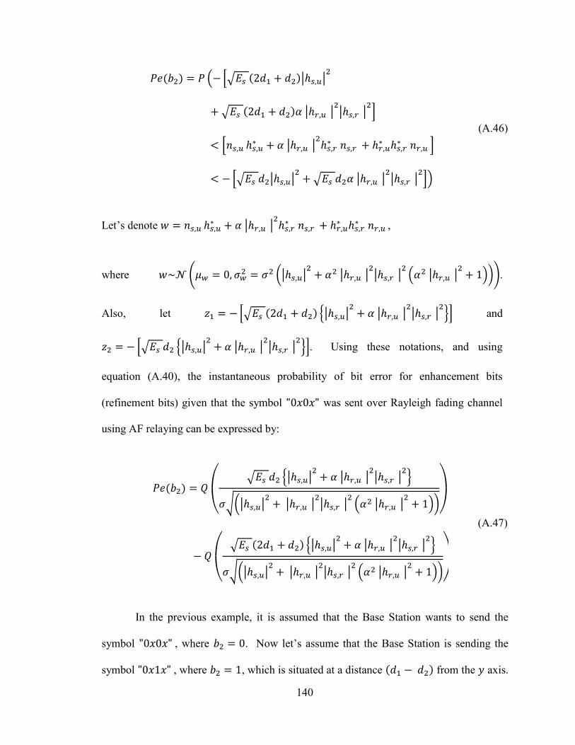
140
( [√ |ℎ |
√ |ℎ | |ℎ |
]
[ ℎ |ℎ |
ℎ ℎ
ℎ ]
[√ |ℎ | √ |ℎ |
|ℎ |
])
(A.46)
Let’s denote ℎ |ℎ |
ℎ ℎ
ℎ ,
where ( (|ℎ |
|ℎ |
|ℎ |
( |ℎ |
))).
Also, let [√ {|ℎ | |ℎ |
|ℎ |
}] and
[√ {|ℎ | |ℎ |
|ℎ |
}]. Using these notations, and using
equation (A.40), the instantaneous probability of bit error for enhancement bits
(refinement bits) given that the symbol was sent over Rayleigh fading channel
using AF relaying can be expressed by:
(
√ {|ℎ |
|ℎ |
|ℎ |
}
√(|ℎ | |ℎ |
|ℎ |
( |ℎ |
))
)
(
√ {|ℎ |
|ℎ |
|ℎ |
}
√(|ℎ | |ℎ |
|ℎ |
( |ℎ |
))
)
(A.47)
In the previous example, it is assumed that the Base Station wants to send the
symbol , where . Now let’s assume that the Base Station is sending the
symbol , where , which is situated at a distance from the axis.
141
The probability of getting an error in such a case, i.e. the reception of a 0, means that the
resulting symbol from combining the two signals coming from the BS and from the relay
leads to a reception of signal in the region. In other words, if the resultant
received signal is denoted by the probability of error can be expressed as
( ℎ ) ( ℎ) (A.48)
The received signals from the Base Station in the first time slot at the destination
and at the relay respectively are
√ ℎ (A.49)
√ ℎ (A.50)
where and denote the selected distance parameters in the first time slot.
a) DF Relaying Case
If the CRC check results in successful decoding, the relay re-modulates its signal with
new constellation’s distance parameters and re-sends its signal. At the destination, the
received signal from the relay is expressed as
√
ℎ (A.51)
ℎ is the fading channel coefficient on the relay-destination link and is the AWGN
coefficient at the destination.
denote the selected distance parameters in the
second time slot.
142
The two signals and are combined at the destination using MRC
technique. The resultant signal is given by:
√ |ℎ |
ℎ
√
|ℎ |
ℎ
(A.52)
Thus, from equations (A.48) and (A.52) the probability of error for the bit in the
symbol can be written as follow:
( [√ |ℎ | √
|ℎ | ]
[√ |ℎ | ℎ
√
|ℎ |
ℎ
])
([√ |ℎ | √
|ℎ | ]
[√ |ℎ | ℎ
√
|ℎ |
ℎ
])
(A.53)
([√ |ℎ | √
|ℎ |
]
[ ℎ ℎ
])
([√ |ℎ | √
|ℎ | ] [ ℎ
ℎ ])
(A.54)
143
Let’s denote ℎ ℎ
, where ( (|ℎ |
|ℎ | )). Also, let [√ |ℎ |
√
|ℎ |
] and
[√ |ℎ | √
|ℎ | ]. Using these notations and using equation (A.54)
(
) (
) (A.55)
Thus the instantaneous probability of bit error for enhancement bits (refinement bits)
given that the symbol was sent over Rayleigh fading channel can be expressed
by:
(
√ |ℎ |
√
|ℎ |
√(|ℎ | |ℎ |
)
)
(
√ |ℎ |
√
|ℎ |
√(|ℎ | |ℎ |
)
)
(A.56)
b) AF Relaying Case
After the relay amplifies the signal and re-sends it, the received signal at the destination
from the relay is given by
ℎ (A.57)
144
ℎ ℎ √ ℎ
(A.58)
where ℎ is the fading channel coefficient on the relay-destination link and is the
AWGN coefficient at the destination. The two signals and are combined at the
destination using Maximal Ratio Combining technique. The resultant signal is given
by:
√ |ℎ | ℎ
√ |ℎ | |ℎ |
|ℎ | ℎ ℎ
ℎ
(A.59)
Thus, from equations (A.48) and (A.59) the probability of error for the bit in the
symbol using AF relaying can be written as follow:
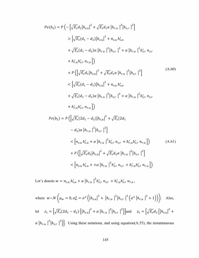
145
( [√ |ℎ | √ |ℎ |
|ℎ |
]
[√ |ℎ | ℎ
√ |ℎ | |ℎ |
|ℎ |
ℎ
ℎ ℎ
])
([√ |ℎ | √ |ℎ |
|ℎ |
]
[√ |ℎ | ℎ
√ |ℎ | |ℎ |
|ℎ |
ℎ
ℎ ℎ
])
(A.60)
([√ |ℎ | √
|ℎ | |ℎ |
]
[ ℎ |ℎ |
ℎ ℎ
ℎ ])
([√ |ℎ | √ |ℎ |
|ℎ |
]
[ ℎ |ℎ |
ℎ ℎ
ℎ ])
(A.61)
Let’s denote ℎ |ℎ |
ℎ ℎ
ℎ ,
where ( (|ℎ |
|ℎ |
|ℎ |
( |ℎ |
))). Also,
let [√ {|ℎ | |ℎ |
|ℎ |
}]and [√ {|ℎ |
|ℎ | |ℎ |
}]. Using these notations, and using equation(A.55), the instantaneous
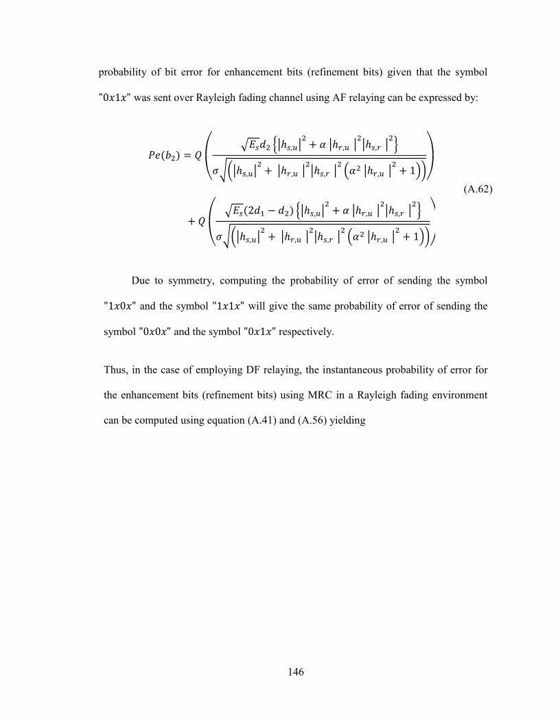
146
probability of bit error for enhancement bits (refinement bits) given that the symbol
was sent over Rayleigh fading channel using AF relaying can be expressed by:
(
√ {|ℎ |
|ℎ |
|ℎ |
}
√(|ℎ | |ℎ |
|ℎ |
( |ℎ |
))
)
(
√ {|ℎ |
|ℎ |
|ℎ |
}
√(|ℎ | |ℎ |
|ℎ |
( |ℎ |
))
)
(A.62)
Due to symmetry, computing the probability of error of sending the symbol
and the symbol will give the same probability of error of sending the
symbol and the symbol respectively.
Thus, in the case of employing DF relaying, the instantaneous probability of error for
the enhancement bits (refinement bits) using MRC in a Rayleigh fading environment
can be computed using equation (A.41) and (A.56) yielding
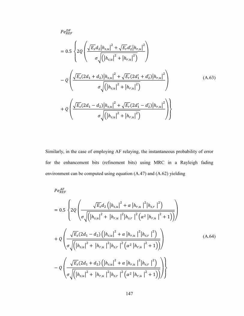
147
{
(
√ |ℎ |
√
|ℎ |
√(|ℎ | |ℎ |
)
)
(
√ |ℎ |
√
|ℎ |
√(|ℎ | |ℎ |
)
)
(
√ |ℎ |
√
|ℎ |
√(|ℎ | |ℎ |
)
)
}
(A.63)
Similarly, in the case of employing AF relaying, the instantaneous probability of error
for the enhancement bits (refinement bits) using MRC in a Rayleigh fading
environment can be computed using equation (A.47) and (A.62) yielding
{
(
√ (|ℎ |
|ℎ |
|ℎ |
)
√(|ℎ | |ℎ |
|ℎ |
( |ℎ |
))
)
(
√ (|ℎ |
|ℎ |
|ℎ |
)
√(|ℎ | |ℎ |
|ℎ |
( |ℎ |
))
)
(
√ (|ℎ |
|ℎ |
|ℎ |
)
√(|ℎ | |ℎ |
|ℎ |
( |ℎ |
))
)
}
(A.64)
148
Bibliography
[1] S.-Y. Li, R. Yeung and N. Cai, "Linear network coding," IEEE Trans. Inf Theory,
vol. 49, no. 2, pp. 371-381, February 2003.
[2] C. Fragouli, J. Le Boudec and J. Widmer, "Network coding: an instant primer,"
ACM SIGCOMM Computer Communication Review Newsletter, vol. 36, no. 1, pp.
63-68, Jan. 2006.
[3] S. Zhang, S. Liew and P. Lam, "Physical layer network coding," in ACM
MOBICOM, 2006.
[4] R. Koetter and M. Medard, "An algebric approach to network coding," IEEE/ACM
Trans. on Networking, vol. 11, no. 5, pp. 782-795, Oct. 2003.
[5] T. Cover, "Broadcast channels," IEEE Trans. Info. Theory, Vols. IT-18, no. 1, pp.
2-14, Jan. 1972.
[6] E. Lo and K. Letaief, "Network coding versus superposition coding for two-way
wireless communication," in IEEE Wireless Communications and Networking
Conference,2009. WCNC 2009, 2009.
[7] B. Choi, S. Boppana and J. Shea, "Superposition coding and linear network coding
for reliable multicasting over fading channels," in IEEE Military Communications
Conf. 2008. MILICOM 2008., 2008.
[8] B. Choi, S. Boppana and J. Shea, "Superposition coding and network coding for
mixed multicast/unicast traffic on a time varying channel," in IEEE Military
Communications Conf. 2009. MILICOM 2009., 2009.
[9] L.-F. Wei, "Coded modulation with unequal error protection," IEEE Trans. on
Commun., vol. 41, no. 10, pp. 1439-1449, Oct. 1993.
[10] M.-K. Chang and S.-Y. Lee, "Performance analysis of cooperative communication
system with hierarchical modulation over Rayleigh fading channel," IEEE Trans.
Wireless Commun., vol. 8, no. 6, pp. 2848-2852, June 2009.
[11] R. Whang, H. Liu and E.-K. Hong, "Multiuser cooperative relay communication
employing hierarchical modulation," in IEEE 71st Vehicular Technology
Conf.,2010. VTC 2010-Spring, 2010.
149
[12] J. Proakis, Digital communications, 4th ed., McGraw-Hill, 2000.
[13] T. Duman and A. Ghrayeb, Coding for MIMO Communication Systems, Wiley &
Sons, 2008.
[14] E. V. D. Meulen, "Three terminal communication channels," Adv. in Appl. Prob.,
vol. 3, no. 1, pp. 120-154, 1971.
[15] T. Cover and A. Gamal, "Capacity theorems for the relay channel," IEEE Trans.
Inf. Theory, vol. 25, no. 5, pp. 572-584, September 1979.
[16] G. Kramer, M. Gastpar and P. Gupta, "Cooperative strategies and capacity
theorems for relay networks," IEEE Trans. Inf. Theory, vol. 51, no. 9, pp. 3037-
3063, September 2005.
[17] G. Kramer, M. Gastpar and P. Gupta, "Capacity theorems for wireless relay
channels," in 41th Allerton Conf. on Commun., Control and Computing, 2003.
[18] A. Sendonaris, E. Erkip and B. Aazhang, "User cooperation diversity part I: System
description," IEEE Trans. Commun., vol. 51, no. 11, pp. 1927-1938, Nov. 2003.
[19] A. Sendonaris, E. Erkip and B. Aazhang, "User cooperation diversity part II:
Implementation aspects and performance analysis," IEEE Trans. Commun., vol. 51,
no. 11, pp. 1939-1948, November 2003.
[20] S. Nguyen, A. Ghrayeb, G. Al-Habian and M. Hasna, "Mitigating error propagation
in two-way relay channels with network coding," IEEE Trans. on Wireless
Commun., vol. 9, no. 11, pp. 3380-3390, Nov. 2010.
[21] J. N. Laneman, D. N. C. Tse and G. W. Wornell, "Cooperative diversity in wireless
networks: Efficient protocols and outage behavior," IEEE Trans. Inf. Theory, vol.
50, no. 12, pp. 3062-3080, December 2004.
[22] X. Zhang, A. Ghrayeb and M. Hasna, "Relay assignment schemes for multiple
source destination cooperative networks," 2010.
[23] Y. Zhao, R. Adve and T. Lim, "Symbol error rate of selection amplify and forward
relay systems," IEEE Commun. Lett., vol. 10, no. 11, pp. 757-759, November 2006.
[24] M. Hasna and M.-S. Alouini, "End to end performance of transmission systems
with relays over Rayleigh fading channels," IEEE Trans. Wireless Commun., vol.
2, no. 6, pp. 1126-1131, November 2003.
150
[25] Y. Hu, K. H. Li and K. C. Teh, "Performance of two way amplify and forward
relay networks over asymmetric channels," 2009.
[26] M. Elfituri, A. Ghrayeb and W. Hamouda, "Antenna/relay selection for coded
cooperative networks with AF relaying," IEEE Trans. Commun., vol. 57, no. 9, pp.
2580-2584, September 2009.
[27] B. Rankov and A. Wittneben, "Achievable rate regions for the two-way relay
channel," in IEEE Int. Symp. On Information Theory, 2006.
[28] A. Bletsas, H. Shin and M. Win, "Outage-optimal cooperative communications
with regenerative relays," in 40th Annu. Conf. on Information Sciences and
Systems., 2006.
[29] L. Zhang and L. Chimini, "Cooperative network coding in selective decode and
forward networks with multiple source destination pairs," in 42nd Annu. Conf. on
Information Sciences and Systems, 2008.
[30] P. Herhold, E. Zimmermann and G. Fettweis, "A simple cooperative extension to
wireless relaying," in Int. Zurich Seminar on Communications, 2004.
[31] M. Xiao and M. Skoglund, "Design of Network codes for multiple-user multiple
relay wireless networks," in IEEE Int. Symp. on Information Theory, 2009.
[32] J. Zhao, M. Kuhn, A. Wittneben and G. Bauch, "Cooperative transmission schemes
for decode and forward relaying," in 18th Int. Symp. on Personal, Indoor and
Mobile Radio Communications, 2007. PIMRC 2007., 2007.
[33] H. Khuong and H. Kong, "LLR based decode and forward protocol for relay
networks and closed form BER expressions," IEICE Trans. on Fundamentals of
Electronics, Communications and Computer Sciences, Vols. E89-A, no. 6, pp.
1832-1841, June 2006.
[34] T. Eng, N. Kong and L. Milstein, "Comparison of diversity combining techniques
for Rayleigh-fading channels," IEEE Trans. Commun., vol. 44, no. 9, pp. 1117-
1129, September 1996.
[35] D. Brennan, "Linear diversity combining techniques," Proceedings of the IEEE,
vol. 91, no. 2, pp. 331-356, 2003.
[36] T. Lo, "Maximum ratio tranmission," IEEE Trans. Commun., vol. 47, no. 10, p.
1999, October 1458-1461.
151
[37] M. K. Simon and M.-S. Alouini, Digital communication over fading channels, 2nd
ed., New York: John Wiley & Sons, 2005.
[38] W. Su, A. Sadek and K. Liu, "Cooperative communication protocols in wireless
networks: performance analysis and optimum power allocation," Wireless
Personnal Communications, vol. 44, no. 2, pp. 181-217, January 2008.
[39] M. Hasna and M.-S. Alouini, "Performance analysis of two-hop relayed
transmissions over Rayleigh fading channels," in IEEE Vehicular Technology
Conference (VHC), 2002.
[40] W. Su, A. Sadek and K. Liu, "SER performance analysis and optimum power
allocation for decode and forward cooperative protocol in wireless networks," in
IEEE Wireless Communications and Networkcing Conference, New Orleans, LA,
2005.
[41] R. C. Palat, A. Annamalai and J. H. Reed, "Log-likelihood-ratio based selective
decode and forward cooperative communication," in IEEE VTC, 2008.
[42] M. R. Souryal, "Performance of Amplify-and-Forward and Decode-and-Forward
Relaying in Rayleigh Fading with Turbo Codes," in IEEE International Conference
on Acoustics, Speech and Signal Processing, 2006. ICASSP 2006 , 2006.
[43] Y. Jia and A. Vosoughi, "A novel selective relaying protocol for wireless
networks," in IEEE 10th Workshop on Signal Processing Advances in Wireless
Communications, 2009. SPAWC '09. , 2009.
[44] M. Elfituri, W. Hamouda and A. Ghrayeb, "A convolutional based coded
cooperation scheme for relay channels," IEEE Trans. Veh. Technol., vol. 58, pp.
655-669, Feb. 2009.
[45] Y. Wang, C. Hu, H. Liu, M. Peng and W. Wang, "Network coding in cooperative
relay networks," in 19th Int. Symp. on Personal, Indoor and Mobile Radio
Communications, 2008. PIMRC 2008., 2008.
[46] Y. Wu, P. A. Chou and S.-Y. Kung, "Information exchange in wireless networks
with network coding and physical layer broadcast," Redmond, WA, 2004.
[47] P. P. Bergmans and T. M. Cover, "Cooperative broadcasting," IEEE Tran. Inf.
Theory, Vols. IT-20, pp. 317-324, May 1974.
[48] K. Fazel and M. Ruf, "Combined multilevel coding and mutliresolution
152
modulation," in IEEE Int. Conf. on Communications, 1993. ICC 93., Geneva, 1993.
[49] ETSI, "Digital Video Broadcasting (DVB): Framing structure, channel coding and
modulation for digital terrestrial television," Nov. 2004.
[50] R. Ahlswede, N. Cai, S.-Y. Li and R. Yeung, "Network information flow," IEEE
Trans. Inf. Theory, vol. 46, no. 4, pp. 1204-1216, Jul 2000.
[51] Y. Chen, S. Kishore and J. Li, "Wireless diversity through network coding," in
IEEE Wireless Communications and Networking Conf.,2006. WCNC 2006., 2006.
[52] P. Larsson, N. Johansson and K.-E. Sunell, "Coded bi-directed relaying," in IEEE
63rd Vehicular Technology Conf.,2006. VTC 2006-Spring., 2006.
[53] S. Yang and R. Koetter, "Network coding over a noisy relay: a belief propagation
approach," in IEEE Int. Symp. on Information Technology, 2007.
[54] M. Xiao and T. Aulin, "Optimal decoding and performance analysis of a noisy
channel network with network coding," IEEE Trans. Commun., vol. 57, no. 5, pp.
1402-1412, May 2009.
[55] P. Popovski and H. Yomo, "Bi-directional amplification of throughput in a wireless
multi-hop network," in IEEE 63rd Vehicular Technology Conference, 2006. VTC
2006-Spring., 2006.
[56] P. Popovski and H. Yomo, "Wireless network coding by amplify-and-forward for
bi-directional traffic flows," IEEE Commun. Letters, vol. 11, no. 1, pp. 16-18, Jan.
2007.
[57] P. Popovski, "The Anti-Packets Can Increase the Achievable Throughput of a
Wireless Multi-Hop Network," in IEEE International Conference on
Communications, 2006. ICC '06., 2006.
[58] M. Park and S. K. Oh, "A Hybrid Network-Superposition Coding for Asymmetrical
Two-Way Relay Channels," in IEEE 70th Vehicular Technology Conference. VTC
2009-Fall., 2009.
[59] C. Liu and A. Arapostathis, "Joint network coding and superposition coding for
multi-user information exchange in wireless relaying networks," in IEEE Global
Telecommunications Conf.,2008. GLOBECOM 2008., 2008.
[60] E. Larsson and B. Vojcic, "Cooperative transmit diversity based on superposition
153
modulation," IEEE Communications Letters, vol. 9, no. 9, pp. 778-780, Sept 2005.
[61] L. Xiao, T. Fuja, J. Kliewer and D. Costello, "Cooperative diversity based on code
superposition," in IEEE International Symposium on Information Theory, 2006,
2006.
[62] L. Xiao, T. Fuja, J. Kliewer and D. Costello, "A network coding approach to
cooperative diversity," IEEE Trans. Inf. Theory, vol. 53, no. 10, pp. 3714-3722,
Oct. 2007.
[63] L. Xiao, T. Fuja, J. Kliewer and D. Costello, "Signal superposition coded
cooperative diversity: analysis and optimization," in IEEE Information Theory
Workshop, 2007. ITW '07., 2007.
[64] A. Goparaju, S. Wei and Y. Liu, "On Superposition coding based cooperative
diversity schemes," in Conference Record of the Thirty-Ninth Asilomar Conference
on Signals, Systems and Computers, 2005. , 2005.
[65] P. Popovski and E. de Carvalho, "Spectrally efficient wireless relaying based on
superposition coding," in IEEE 65th Vehicular Technology Conf.,2007. VTC 2007-
Spring., 2007.
[66] L. Chen, L. Cao, X. Zhang and D. Yang, "Integrating network coding and
superposition coding in extended two-way relay networks," in IEEE GLOBECOM
Workshops (GC Wkshps), 2010., 2010.
[67] J. Park, S.-L. Kim and J. Choi, "Hierarchically modulated network coding for
asymmetric two-way relay systems," IEEE Trans. Veh Technol, vol. 59, no. 5, pp.
2179-2184, June 2010.
[68] P. K. Vitthaladevuni and M.-S. Alouini, "BER computation of 4/M-QAM
hierarchical constellations," IEEE Trans. Broadcasting, vol. 47, no. 3, pp. 228-239,
September 2001.
[69] C. Hausl and J. Hagenauer, "Relay communication with hierarchical modulation,"
IEEE Commun. Lett., vol. 11, no. 1, pp. 64-66, January 2007.
[70] J.-C. Shin, J.-H. Kim, J.-H. Song and H.-K. Song, "New transmission scheme with
hierarchical modulation in dual-hop wireless relaying systems," in 2009
Australasian Telecommunication Networks and Applications Conf. (ATNAC), 2009.
[71] R. Y. Kim and Y. Y. Kim, "Symbol-level random network coded cooperation with

154
hierarchical modulation in relay communication," IEEE Trans. Consumer
Electronics, vol. 55, no. 3, pp. 1280-1285, Aug. 2009.
[72] A. Bin Sediq, P. Djukic, H. Yanikomeroglu and J. Zhang, "Generalized
constellation rearrangement in cooperative relaying," in IEEE 71st Vehicular
Technology Conference, VTC 2010-Spring., 2010.
[73] H. Nguyen, H. Nguyen and L.-N. Tho, "Signal transmission with unequal error
protection in wireless relay networks," IEEE Trans. Vehicular Technology, vol. 59,
no. 5, pp. 2166-2178, June 2010.
[74] C. Berrou, A. Glavieux and P. Thitimajshima, "Near Shanon limit error correcting
coding and decoding: Turbo codes," in IEEE Proceedings of the Int. Conf. on
Communications, Geneva, 1993.
[75] C. Berrou and A. Glavieux, "Near optimum error correcting coding and decoding:
Turbo codes," IEEE Trans. Commun., vol. 44, no. 10, pp. 1261-1271, October
1996.
[76] R. Pyndiah, P. Combelles and P. Adde, "A very low complexity block turbo
decoder for product codes," in IEEE Global Telecommunications Conf., 1996.
GLOBECOM '96., 1996.
[77] P. Ferry, c. Adde and G. Graton, "Turbo decoder synchronization procedure:
application to the CAS5093 integrated circuit," in Proceedings of the Third IEEE
Int. Conf. on Electronics, Circuits and Systems, 1996. ICECS '96., 1996.
[78] C. Berrou, Practical considerations on turbo-codes, KPN Research, La haye, 1996.
[79] C. Berrou and A. Glavieux, "Turbo-codes, general principles and applications," in
6th Int. Tirrenia Workshop on Digital Communications, Pisa, 1993.
[80] C. Berrou, A. Glavieux and R. Pyndiah, "Turbo-codes: principe et applications," in
GRETSI '95, Juan Les Pins, 1995.
[81] M. Valenti, "Turbo codes and iterative processing," in IEEE New Zealand Wireless
Commun. Symp., Auckland, 1998.
[82] B. Sklar, "A primer on Turbo Code concepts," IEEE Commun. Magazine, vol. 35,
no. 12, pp. 94-102, Dec. 1997.
[83] M. C. Valenti and J. Sun, "The UMTS Turbo code and an efficient decoder
155
implementation suitable for software defined radios," International Journal of
Wireless Information Networks, vol. 8, no. 4, pp. 203-215, October 2002.
[84] C. Berrou, S. Evano and G. Battail, "Turbo block codes," in Turbo coding seminar,
Sweden, 1996.
[85] P. Adde, R. Pyndiah and O. Raoul, "Performance and complexity of block turbo
decoder circuit," in 3rd Int. Conf. on Electronics, Circuits and System, 1996.
ICECS '96., Rodos, 1996.
[86] M. Jezequel, C. Berrou, C. Douillard and P. Penard, "Characteristics of a sixteen-
state turbo encoder/decoder (turbo4)," in Int. Symp. on Turbo codes and Related
Topics, Brest, 1997.
[87] C. Berrou, M. Jezequel and C. Douillard, "Multidimensional Turbo codes," in
Information Theory and Networking Workshop, Metsovo, 1999.
[88] C. Berrou and M. Jezequel, "Non-binary convolutional codes for turbo coding,"
Electronics letters, vol. 35, no. 1, pp. 39-40, January 1999.
[89] K. Sripimanwat, Turbo code applications, a journey from a paper to realization,
Dordrecht: Springer, 2005.
[90] M. Valenti, "Iterative detection and decoding for wireless communications,"
Virginia, USA, 1999.
[91] S. Lin and D. J. Costello, Error Control Codes, New Jersey: Prentice Hall, 2004.
[92] M. R. Soleymani, Y. Gao and U. Vilaipornsawai, Turbo coding for satellite and
wireless communications, MA: Kluwer Academic Publishers, 2002.
[93] G. D. Forney, "The Viterbi algorithm," Proceedings of the IEEE, vol. 61, no. 3, pp.
268-278, March 1973.
[94] L. R. Bahl, J. Cocke, F. Jelinek and J. Raviv, "Optimal decoding of linear codes for
minimizing symbol error rate," IEEE Trans. Inf. Theory, vol. 20, no. 2, pp. 284-
287, March 1974.
[95] K. Abend and B. Fritchman, "Statistical detection for communication channels with
intersymbol interference," in Proc. IEEE, 1970.
[96] Y. Li, B. Vucetic and Y. Sato, "Optimum soft output detection for channels with
156
intersymbol interference," IEEE Trans. Inf. Theory, vol. 41, no. 3, pp. 704-713,
May 1995.
[97] P. Robertson, P. Hoeher and E. Villebrun, "Optimal and Sub-Optimal Maximum A
Posteriori Algorithms Suitable for Turbo Decoding," European Trans. on
Telecommun., vol. 8, pp. 119-125, April 1997.
[98] S. Le Goff, A. Glavieux and C. Berrou, "Turbo-codes and high spectral efficiency
modulation," in IEEE Int. Conf. on Communications, 1994. ICC '94., 1994.
[99] P. Dong, P. Fan and L. Yi, "Iterative phase recovery method of turbo coded 16
QAM based on soft symbol to bit mapping," in The 2004 Joint Conference of the
10th Asia-Pacific Conference on Communications, 2004 and the 5th International
Symposium on Multi-Dimensional Mobile Communications Proceedings. , 2004.
[100] C. C. Wang and Q. Vo, "Unequal protection with Turbo decoding for high order
modulated signaling," in IEEE Wireless Communications and Networking
Conference, 2005, 2005.
[101] N. H. Ngo, S. S. Pietrobon, S. S. Pietrobon and S. A. Barbulescu, "A New Iterative
Decoder for Turbo Codes on the Nonlinear Channel with Non-uniform 16QAM
Modulation," in 4th International Symposium on Turbo Codes&Related Topics; 6th
International ITG-Conference on Source and Channel Coding (TURBOCODING),
2006 , 2006.
[102] M. Aydinlik and M. Salehi, "Turbo Coded Modulation for Unequal Error
Protection," IEEE Transactions on Communications, vol. 56, no. 4, pp. 555-564,
April 2008.
[103] K. Lee, D. Kang, H. Park and W. Oh, "Joint encoding and modulation scheme for
binary Turbo code and 16QAM," in The 6th International Conference on
Information Technology and Applications (ICITA 2009), 2009.
[104] X. Zhe, W. Yongsheng, F. Alberge and P. Duhamel, "A turbo iteration algorithm in
16QAM hierarchical modulation," in 2010 IEEE International Conference on
Wireless Communications, Networking and Information Security (WCNIS), 2010.
[105] P. Vitthaladevuni and M.-S. Alouini, "A recursive algorithm for the exact BER
computation of generalized hierarchical QAM constellations," IEEE Trans. Inf.
Theory, vol. 49, no. 1, pp. 297- 307, Jan. 2003.
157
[106] H. V. Khuong and H. Y. Kong, "LLR-based decode and forward protocol for relay
networks and closed form BER expressions," IEICE Trans. Fundamentals, vol.
E89A, pp. 1832-1841, June 2006.
[107] C. Fragouli, J.-Y. Le Boudec and J. Widemer, "Network coding: an instant primer,"
ACM SIGCOMM Computer Communication Review, vol. 36, no. 1, pp. 63-68, Jan.
2006.
[108] R. Koetter and M. Medard, "An algebric approach to network coding," IEEE/ACM
Trans. on Networking, vol. 11, no. 5, pp. 782-795, October 2003.
[109] C.-H. Liu and A. Arapostathis, "Joint Network Coding and Superposition Coding
for Multi-User Information Exchange in Wireless Relaying Networks," in IEEE
Global Telecommunications Conference, 2008. IEEE GLOBECOM 2008., 2008.
[110] T. M. Cover, "Broadcast channels," IEEE Trans. Inf. Theory, vol. 18, no. 1, pp. 2-
14, Jan 1972.
[111] E. S. Lo and K. B. Letaief, "Network Coding Versus Superposition Coding for
Two-Way Wireless Communication," in IEEE Wireless Communications and
Networking Conference, 2009. WCNC 2009. , 2009.
[112] K. Fazel and M. Ruf, "Combined multilevel coding and multiresolution
modulation," in IEEE Int. Conf. on Communication,1993. ICC 93., 1993.
[113] K. Fazel and M. Ruf, "A hierarchical digital HDTV transmission scheme for
terrestrial broadcasting," in IEEE Global Telecommunication Conf.,1993.
GLOBECOM 93., Houston, 1993.
[115] T. Wang, A. Cano, G. Giannakis and F. Ramos, "Multi-tiers cooperative
broadcasting with hierarchical modulations," IEEE Trans. Wireless Commun., vol.
6, no. 8, pp. 3047-3057, August 2007.
[116] E. Larson and B. Vojcic, "Cooperative transmit diversity based on superposition
modulation," IEEE Commun. Lett., vol. 9, no. 9, pp. 778-780, September 2005.
[117] T. Hunter and A. Nasratinia, "Cooperation diversity through coding," in IEEE Int.
Symp. on Information Theory, 2002.
[118] C. Berrou and P. Combelles, "Digital television: hierarchical channel coding using
turbo codes," in IEEE Int. Conf. on Communications, 1994. ICC '94., New Orleans,
1994.
158
[119] L.-L. Yang and L. Hanzo, "A recursive algorithm for the error probability
evaluation of M-QAM," IEEE Commun. Lett., vol. 4, no. 10, pp. 304-306, October
2000.
[120] D. Yoon, K. Cho and J. Lee, "Bit error probability of M-ary quadrature amplitude
modulation," in 52nd IEEE Vehicular Technology Conference, 2000. VTS-Fall
2000. , 2000.
[121] C. Berrou and A. Glaviex, "Near optimum error correcting coding and decoding:
Turbo codes," IEEE Trans. Commun., vol. 44, no. 10, pp. 1261-1271, October
1996.
[122] A. Sendonaris, E. Erkip and B. Aazhang, " User cooperation diversity part I:
System description," IEEE Trans. Commun., vol. 51, no. 11, pp. 1927-1938,
November 2003.
[123] D. Brennan, "Linear diversity combining techniques," Proceedings of the IRE, vol.
49, pp. 1075-1101, June 1959.
[124] C. Berrou, Practical considerations on turbo-codes, KPN Research, la haye, 1996.
[125] Y. Jia and A. Vosoughi, "A novel selective relaying protocol for wireless
networks," in IEEE 10th Workshop on Signal Processing Advances in Wireless
Communications, 2009. SPAWC '09., 2009.